11institutetext: Institute for Advanced Study, Princeton, NJ 08540, USA22institutetext: Jefferson Physical Laboratory, Harvard University, Cambridge, MA 02138, USA33institutetext: Department of Mathematics, Harvard University, Cambridge, MA 02138, USA44institutetext: Department of Physics and Astronomy and Center for Theoretical Physics, Seoul National University, Seoul 151-747, Korea.

6d String Chains

Abhijit Gadde 2,3    Babak Haghighat 4    Joonho Kim 4    Seok Kim 2    Guglielmo Lockhart 2    Cumrun Vafa
Abstract

We consider bound states of strings which arise in 6d (1,0) SCFTs that are realized in F-theory in terms of linear chains of spheres with negative self-intersections 1,2, and 4. These include the strings associated to N𝑁N small E8subscript𝐸8E_{8} instantons, as well as the ones associated to M5 branes probing A and D type singularities in M-theory or D5 branes probing ADE singularities in Type IIB string theory. We find that these bound states of strings admit (0,4) supersymmetric quiver descriptions and show how one can compute their elliptic genera.

1 Introduction

Recently considerable progress has been made in classifying and understanding basic properties of six-dimensional superconformal field theories Heckman:2013pva ; Ohmori:2014pca ; Ohmori:2014kda ; DelZotto:2014hpa ; Heckman:2014qba ; Intriligator:2014eaa ; DelZotto:2014fia ; Heckman:2015bfa ; Bhardwaj:2015xxa ; DelZotto:2015isa ; Miao:2015iba ; Ohmori:2015pua ; Haghighat:2013gba ; Haghighat:2013tka ; Haghighat:2014pva ; Kim:2014dza ; Haghighat:2014vxa . Formulating these theories in a way which leads to a computational scheme of physical amplitudes is still a major challenge. One idea along these lines is to note that on their tensor branch these theories have light strings as basic ingredients, which naturally suggests that these strings should play a key role in any computational scheme. For example, it is already known that their elliptic genus can be used to compute the superconformal index of these 6d theories Lockhart:2012vp ; Kim:2012qf ; Haghighat:2013gba . The main aim of this paper is to expand the known dictionary Haghighat:2013gba ; Haghighat:2013tka ; Kim:2014dza ; Haghighat:2014vxa for describing the degrees of freedom living on these strings.

The six-dimensional SCFTs that can be obtained via F-theory compactification were classified in Heckman:2013pva ; DelZotto:2014hpa ; Heckman:2015bfa (see also Bhardwaj:2015xxa ). This includes all presently known 6d SCFTs, and it may well be the case that all consistent 6d SCFTs can be realized this way. In this context, six-dimensional SCFTs are realized by putting F-theory on elliptic Calabi-Yau threefold with a non-compact base B𝐵B with the property that all compact curves can be simultaneously contracted to zero size. These curves are in fact two-spheres that have negative self-intersection ranging from 1 to 12 (excluding 9,10,11) and intersect one another at a point, and are arranged into trees according to specific rules. In particular, one can identify some basic building blocks (the curves with negative self-intersection 3,,8383,\dots,8 and 12, and a few combinations of two or three curves Morrison:2012np ) that can be glued together by joining them with (1)1(-1)-curves. Each curve gives rise to a tensor multiplet in the 6d theory. D3 branes wrapping a curve correspond to strings coupled to the corresponding tensor multiplet. Furthermore, gauge multiplets arise whenever the elliptic fiber degenerates over a curve, the nature of the resulting gauge group being determined by the type of degeneration. In particular, non-Higgsable clusters necessarily support a nontrivial gauge group, whose rank can be made larger by increasing the degree of the singularity.

Under favorable circumstances, bound states of strings admit a description in terms of a two-dimensional (0,4) quiver gauge theory. In this paper we extend the list of theories for which such a description is available to three additional classes of 6d SCFTs:

  • The theory of M5 branes probing a singularity of A or D type. The first case was studied in Haghighat:2013tka and corresponds to a linear chain of (2)2(-2) curves and leads to a 6d theory with SU-type gauge group; the second case is novel and corresponds to a linear chain of alternating (1)1(-1) and (4)4(-4) curves which support respectively gauge group SO(8+2p)𝑆𝑂82𝑝SO(8+2p) and Sp(p)𝑆𝑝𝑝Sp(p).

  • The theory of N𝑁N small E8subscript𝐸8E_{8} instantons, or equivalently N𝑁N M5 branes probing the M9 plane of Hořava-Witten theory Seiberg:1996vs ; Ganor:1996mu . This corresponds to a single (1)1(-1) curve linked to a chain of N1𝑁1N-1 curves of self-intersection 22-2. Upon circle compactification, this theory admits deformation by a parameter corresponding to the mass of a 5d anti-symmetric hypermultiplet. We focus on the case where this parameter is turned off.

  • The theory of N𝑁N D5 branes probing an ADE singularity. This corresponds in F-theory to an ADE configuration of 22-2 curves supporting gauge groups of SU𝑆𝑈SU type.

Once the quiver gauge theory corresponding to a given configuration of strings is specified, the elliptic genus can be computed by means of localization Gadde:2013dda ; Benini:2013xpa . We do this for certain specific bound states of strings for the first two classes of theories, and for arbitrary bound states of strings for the third class.

The organization of this paper is as follows: In Section 2 we review some of the building blocks for the (0,4) supersymmetric 2d quiver gauge theories which will be needed for the description of the worldsheet degrees of freedom of the tensionless strings. In Section 3 we discuss the 2d quiver for the strings of the theory of M5 branes probing A- or D- type singularities. In Section 4 we study the quiver for the strings of the theory of N𝑁N small E8subscript𝐸8E_{8} instantons. In Section 5 we discuss the quiver for strings of the theory of D5 branes probing an ADE singularity. In Appendix A we discuss a candidate 2d quiver for the strings of the theory of N𝑁N small E8subscript𝐸8E_{8} instantons with mass deformation.

2 Chains of Strings

We are interested in computing the elliptic genera of the strings that arise on tensor branches of 6d (1,0)10(1,0) SCFTs with several tensor multiplets, along the lines of Haghighat:2014vxa , and are wrapped around a torus of complex modulus τ𝜏\tau. In this paper we aim to obtain 2d quiver gauge theories for a variety of 6d SCFTs that arise within M- and F-theory. These will generally consist of (0,4)04(0,4) quiver gauge theories with gauge group i=1NGi(ki)superscriptsubscriptproduct𝑖1𝑁subscript𝐺𝑖subscript𝑘𝑖\prod_{i=1}^{N}G_{i}(k_{i}), where Gisubscript𝐺𝑖G_{i} is the gauge group associated to kisubscript𝑘𝑖k_{i} strings of the i𝑖ith type, and will capture the dynamics of a bound state of such a collection of strings. The gauge groups arising in the theories discussed in this paper are either unitary, symplectic, or orthogonal.

Let us now discuss global symmetries of the 2d (0,4)04(0,4) theory. A number of the global symmetries have a geometric origin, since they arise from rotations of an ||4\mathbb{R}^{4}_{||} along the worldvolume of the six-dimensional theory but transverse to the string’s worldsheet, or from rotations of an 4subscriptsuperscript4perpendicular-to\mathbb{R}^{4}_{\perp} perpendicular to the six-dimensional worldvolume. Overall, an SU(2)4𝑆𝑈superscript24SU(2)^{4} group acting as rotations of ||4×4\mathbb{R}^{4}_{||}\times\mathbb{R}^{4}_{\perp}:

||4\displaystyle\mathbb{R}^{4}_{||} ::\displaystyle: SU(2)A×SU(2)A~,𝑆𝑈subscript2superscript𝐴𝑆𝑈subscript2superscript~𝐴\displaystyle SU(2)_{A^{\prime}}\times SU(2)_{\tilde{A}^{\prime}}~{},
4subscriptsuperscript4perpendicular-to\displaystyle\mathbb{R}^{4}_{\perp} ::\displaystyle: SU(2)A×SU(2)Y.𝑆𝑈subscript2𝐴𝑆𝑈subscript2𝑌\displaystyle SU(2)_{A}\times SU(2)_{Y}. (1)

The right-moving supercharges Q+AAsuperscriptsubscript𝑄𝐴superscript𝐴Q_{+}^{AA^{\prime}} transform under the SO(4)𝑆𝑂4SO(4) R-symmetry given by

SO(4)R=SU(2)A×SU(2)A.𝑆𝑂subscript4𝑅𝑆𝑈subscript2𝐴𝑆𝑈subscript2superscript𝐴SO(4)_{R}=SU(2)_{A}\times SU(2)_{A^{\prime}}. (2)

Let us identify the Cartan of SU(2)4𝑆𝑈superscript24SU(2)^{4} as follows:

U(1)ϵ+×U(1)ϵ×U(1)m×U(1)RSU(2)A×SU(2)A~×SU(2)Y×SU(2)A,𝑈subscript1subscriptitalic-ϵ𝑈subscript1subscriptitalic-ϵ𝑈subscript1𝑚𝑈subscript1𝑅𝑆𝑈subscript2superscript𝐴𝑆𝑈subscript2superscript~𝐴𝑆𝑈subscript2𝑌𝑆𝑈subscript2𝐴U(1)_{\epsilon_{+}}\times U(1)_{\epsilon_{-}}\times U(1)_{m}\times U(1)_{R}\subset SU(2)_{A^{\prime}}\times SU(2)_{\widetilde{A}^{\prime}}\times SU(2)_{Y}\times SU(2)_{A},

where we identify U(1)R𝑈subscript1𝑅U(1)_{R} with the R-symmetry group of the the (0,4)04(0,4) theory when viewed as a (0,2)02(0,2) theory. When computing elliptic genera, we will turn on fugacities ϵ+=12(ϵ1+ϵ2),ϵ=12(ϵ1ϵ2),formulae-sequencesubscriptitalic-ϵ12subscriptitalic-ϵ1subscriptitalic-ϵ2subscriptitalic-ϵ12subscriptitalic-ϵ1subscriptitalic-ϵ2\epsilon_{+}=\frac{1}{2}(\epsilon_{1}+\epsilon_{2}),\epsilon_{-}=\frac{1}{2}(\epsilon_{1}-\epsilon_{2}), and m𝑚m for the remaining U(1)𝑈1U(1) factors in the Cartan.

Below we summarize our notation for the following sections. In drawing quiver diagrams, we will denote (0,2)02(0,2) Fermi multiplets by dashed lines and (0,4)04(0,4) hypermultiplets by a solid line. The various fields of the quiver gauge theory can be organized in terms of four combinations of (0,2) multiplets:

  1. 1.

    To each gauge node i𝑖i corresponds the following field content valued in representations of Gisubscript𝐺𝑖G_{i} (corresponding to nisubscript𝑛𝑖n_{i} strings of the i𝑖ith kind): a vector multiplet ΥisubscriptΥ𝑖\Upsilon_{i}; a Fermi multiplet ΛiΦsuperscriptsubscriptΛ𝑖Φ\Lambda_{i}^{\Phi}; and two chiral multiplets Bi,B~isubscript𝐵𝑖subscript~𝐵𝑖B_{i},\widetilde{B}_{i}.

    Symbol (0,2) field content U(1)ϵ1𝑈subscript1subscriptitalic-ϵ1U(1)_{\epsilon_{1}} U(1)ϵ2𝑈subscript1subscriptitalic-ϵ2U(1)_{\epsilon_{2}} U(1)m𝑈subscript1𝑚U(1)_{m} U(1)R𝑈subscript1𝑅U(1)_{R} Gisubscript𝐺𝑖G_{i}
    [Uncaptioned image] ΥisubscriptΥ𝑖\Upsilon_{i} (vector) 0 0 0 0 adj.
    ΛiΦsuperscriptsubscriptΛ𝑖Φ\Lambda_{i}^{\Phi} (Fermi) 11-1 11-1 0 1 adj.
    B𝐵B (chiral) 1 0 0 0 R
    B~~𝐵\widetilde{B} (chiral) 0 1 0 0 R

    The representation R is the adjoint representation whenever the gauge group is unitary, symmetric whenever the gauge node is orthogonal, and anti-symmetric if the gauge group is symplectic.

  2. 2.

    Between each pair of nodes i,j𝑖𝑗i,j such that the corresponding element of the adjacency matrix of the underlying quiver Mijsubscript𝑀𝑖𝑗M_{ij} is non-zero one has the following bifundamental fields of Gi×Gjsubscript𝐺𝑖subscript𝐺𝑗G_{i}\times G_{j}: two Fermi multiplets ΛijB,ΛijB~subscriptsuperscriptΛ𝐵𝑖𝑗subscriptsuperscriptΛ~𝐵𝑖𝑗\Lambda^{B}_{ij},\Lambda^{\widetilde{B}}_{ij}, and chiral multiplets Φij,ΣijsubscriptΦ𝑖𝑗subscriptΣ𝑖𝑗\Phi_{ij},\Sigma_{ij} forming a twisted (0,4)04(0,4) hypermultiplet.

    Symbol (0,2) field content U(1)ϵ1𝑈subscript1subscriptitalic-ϵ1U(1)_{\epsilon_{1}}​​ U(1)ϵ2𝑈subscript1subscriptitalic-ϵ2U(1)_{\epsilon_{2}}​​ U(1)m𝑈subscript1𝑚U(1)_{m}​​ U(1)R𝑈subscript1𝑅U(1)_{R}​​ Gi×Gjsubscript𝐺𝑖subscript𝐺𝑗G_{i}\!\!\times\!\!G_{j}
    [Uncaptioned image] ΛijBsuperscriptsubscriptΛ𝑖𝑗𝐵\Lambda_{ij}^{B} (Fermi) 1/2 1/212-1/2 1 00 ¯tensor-product¯\square\otimes\overline{\square}
    ΛijB~superscriptsubscriptΛ𝑖𝑗~𝐵\Lambda_{ij}^{\widetilde{B}} (Fermi) 1/212-1/2 1/2 1 00 ¯tensor-product¯\square\otimes\overline{\square}
    ΣijsubscriptΣ𝑖𝑗\Sigma_{ij} (chiral) 1/212-1/2 1/212-1/2 111 1 ¯tensor-product¯\square\otimes\overline{\square}
    ΦijsubscriptΦ𝑖𝑗\Phi_{ij} (chiral) 1/212-1/2 1/212-1/2 -1 1 ¯tensor-product¯\overline{\square}\otimes\square
  3. 3.

    Between each gauge node i𝑖i and the corresponding global symmetry node one has a link corresponding to two chiral multiplets, Q,Q~𝑄~𝑄Q,\widetilde{Q}, charged under Gi×Fisubscript𝐺𝑖subscript𝐹𝑖G_{i}\times F_{i}, where Fisubscript𝐹𝑖F_{i} is the global symmetry group at that node, which we depict by a square in the quiver.

    Symbol (0,2) field content U(1)ϵ1𝑈subscript1subscriptitalic-ϵ1U(1)_{\epsilon_{1}}​​ U(1)ϵ2𝑈subscript1subscriptitalic-ϵ2U(1)_{\epsilon_{2}}​​ U(1)m𝑈subscript1𝑚U(1)_{m}​​ U(1)R𝑈subscript1𝑅U(1)_{R}​​ Gi×Fisubscript𝐺𝑖subscript𝐹𝑖G_{i}\!\!\times\!\!F_{i}
    [Uncaptioned image]
    Qisubscript𝑄𝑖Q_{i} (chiral) 1/2 1/2 0 0 ¯tensor-product¯\square\otimes\overline{\square}
    Q~isubscript~𝑄𝑖\widetilde{Q}_{i} (chiral) 1/2 1/2 0 0 ¯tensor-product¯\overline{\square}\otimes\square
  4. 4.

    Between each gauge node i𝑖i and any successive node j𝑗j one has a Fermi multiplet ΛijQsuperscriptsubscriptΛ𝑖𝑗𝑄\Lambda_{ij}^{Q}; between the same gauge node i𝑖i and any preceding node j𝑗j one has a Fermi multiplet ΛjiQ~superscriptsubscriptΛ𝑗𝑖~𝑄\Lambda_{ji}^{\widetilde{Q}}.

    Symbol ​​ (0,2) field content ​​​ ​​​ U(1)ϵ1𝑈subscript1subscriptitalic-ϵ1U(1)_{\epsilon_{1}}​​ ​​​ U(1)ϵ2𝑈subscript1subscriptitalic-ϵ2U(1)_{\epsilon_{2}}​​ ​​​ U(1)m𝑈subscript1𝑚U(1)_{m}​​ ​​​ U(1)R𝑈subscript1𝑅U(1)_{R} ​​​ ​​​ Gi×Fjsubscript𝐺𝑖subscript𝐹𝑗G_{i}\!\!\times\!\!F_{j}
    [Uncaptioned image]
    ΛijQsubscriptsuperscriptΛ𝑄𝑖𝑗\Lambda^{Q}_{ij} (chiral) 0 0 1 00 ¯tensor-product¯\square\otimes\overline{\square}
    ΛjiQ~subscriptsuperscriptΛ~𝑄𝑗𝑖\Lambda^{\widetilde{Q}}_{ji} (chiral) 0 0 1 00 ¯tensor-product¯\overline{\square}\otimes\square

3 Partition functions of M5 branes probing ADE Singularities

In this section we consider 6d (1,0)10(1,0) SCFTs which arise from M5 branes probing singularities of type A and D, and obtain the 2d quiver gauge theory describing the self-dual strings that arise on the tensor branch of the corresponding 6d theory.

3.1 M5 branes probing an AN1subscript𝐴𝑁1A_{N-1} singularity

Consider a setup where M𝑀M parallel M5 branes span directions X0,,X5superscript𝑋0superscript𝑋5X^{0},\dots,X^{5} and are separated along the X6superscript𝑋6X^{6} direction in 11d spacetime. Taking the transverse space of the M5 branes to be ×2/Nsuperscript2subscript𝑁\mathbb{R}\times\mathbb{C}^{2}/\mathbb{Z}_{N} and blowing up the singular locus gives rise to a (1,0)10(1,0) 6d SCFT on the tensor branch which enjoys a SU(N)×SU(N)𝑆𝑈𝑁𝑆𝑈𝑁SU(N)\times SU(N) flavor symmetry. The AN1subscript𝐴𝑁1A_{N-1} singularity can be thought of as a limit of Taub-NUT space with charge N𝑁N; this space has a canonical circle fibration over 3superscript3\mathbb{R}^{3}, and compactifying M-theory along this circle one arrives at a system of N𝑁N parallel D6-branes stretched between NS5 branes. The dynamics of the strings that arise in this system are captured by the two-dimensional quiver theory of Figure 1:
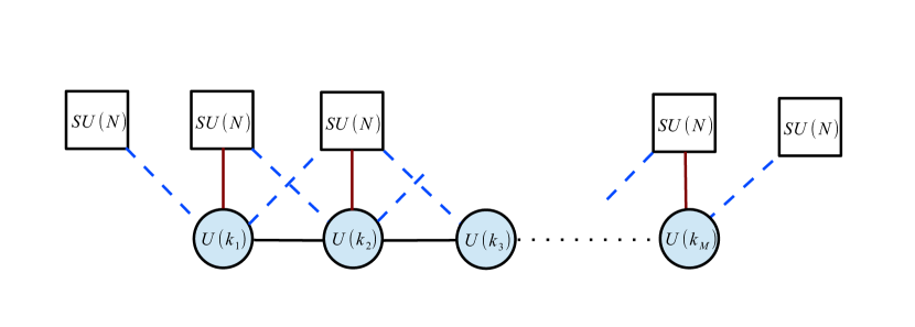
Refer to caption
Figure 1: Non-critical strings in M5 branes probing AN1subscript𝐴𝑁1A_{N-1} singularities.

The quiver corresponds to a 2d 𝒩=(0,4)𝒩04\mathcal{N}=(0,4) theory obtained from a Msubscript𝑀\mathbb{Z}_{M} orbifold of a 𝒩=(4,4)𝒩44\mathcal{N}=(4,4) supersymmetric Yang-Mills theory. As such, each gauge node contains a (0,4)04(0,4) vector multiplet together with an adjoint (0,4)04(0,4) hypermultiplet and the bifundamental fields between the gauge nodes consist of (0,4)04(0,4) Fermi and twisted hypermultiplets. Furthermore, between each gauge node and the adjacent flavor nodes one has (0,2)02(0,2) Fermi multiplets in the fundamental representation of the gauge group and between each gauge node and the corresponding flavor node a fundamental (0,4)04(0,4) hypermultiplet. The exact field content is described in Haghighat:2013tka . Following the rules of Benini:2013xpa and the charge tables of Section 2 one can straightforwardly write down an expression for the elliptic genus for any configuration of strings, corresponding to different choices of the ranks of the gauge groups in the 2d quiver. We will perform the computation in Section 5.

We can also relax the condition that all nodes should have the same SU(N)𝑆𝑈𝑁SU(N) flavor symmetry. In particular, we can consider the situation where the i𝑖ith flavour node has SU(Ni)𝑆𝑈subscript𝑁𝑖SU(N_{i}) symmetry together with the convexity condition

Ni12(Ni1+Ni+1),subscript𝑁𝑖12subscript𝑁𝑖1subscript𝑁𝑖1N_{i}\geq\frac{1}{2}(N_{i-1}+N_{i+1}), (3)

which ensures that the parent 6d theory is not anomalous. In case of equality, all Nisubscript𝑁𝑖N_{i} are ordered along a linear function and gauge anomaly cancellation is automatically satisfied. However, if Nisubscript𝑁𝑖N_{i} is strictly greater than 12(Ni1+Ni+1)12subscript𝑁𝑖1subscript𝑁𝑖1\frac{1}{2}(N_{i-1}+N_{i+1}) the net number of right moving fermions is greater than the number of left-moving ones and the theory will be anomalous. To cure this, we introduce for each gauge node a fourth flavor node with left-moving fermions to compensate for the excess of the right-moving ones. The corresponding quiver is the one depicted in Figure 2.
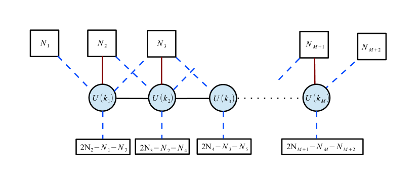
Refer to caption
Figure 2: Convex chain of 22-2 curves.

Again the elliptic genus can be computed straightforwardly using the charge table of Section 2, however one has to be careful with the charge assignments of the new vertical Fermi multiplets: these are not charged under U(1)m,U(1)ϵ+𝑈subscript1𝑚𝑈subscript1subscriptitalic-ϵU(1)_{m},U(1)_{\epsilon_{+}} or U(1)ϵ𝑈subscript1subscriptitalic-ϵU(1)_{\epsilon_{-}}. The origin of the different flavor groups can be explained from the brane construction that corresponds to this theory: one has N1,,NM+2subscript𝑁1subscript𝑁𝑀2N_{1},\dots,N_{M+2} D6 branes separated by NS5 branes. The difference between the number of D6 branes on the two sides of an NS5 brane must equal the negative of the cosmological constant in that region Hanany:1997sa . So, for instance, if we have an NS5 brane with Ni1subscript𝑁𝑖1N_{i-1} D6 branes on the left and Nisubscript𝑁𝑖N_{i} on the right we must have cosmological constant Ni1Nisubscript𝑁𝑖1subscript𝑁𝑖N_{i-1}-N_{i} there. At the next NS5 brane, however, we must have cosmological constant NiNi+1subscript𝑁𝑖subscript𝑁𝑖1N_{i}-N_{i+1}. This is achieved by placing (NiNi+1)(Ni1Ni)=2Ni(Ni1+Ni+1)subscript𝑁𝑖subscript𝑁𝑖1subscript𝑁𝑖1subscript𝑁𝑖2subscript𝑁𝑖subscript𝑁𝑖1subscript𝑁𝑖1(N_{i}-N_{i+1})-(N_{i-1}-N_{i})=2N_{i}-(N_{i-1}+N_{i+1}) D8 branes between the two NS5 branes Hanany:1997gh , which has the effect of changing the cosmological constant as required. This leads to the two-dimensional quiver considered above.

3.2 M5 branes probing a Dp+4subscript𝐷𝑝4D_{p+4} singularity

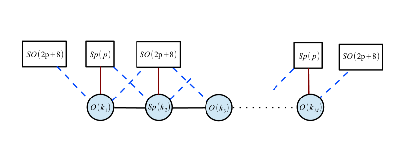
A Dp+4subscript𝐷𝑝4D_{p+4} singularity gives rise to 7d SYM theory with gauge group SO(2p+8)𝑆𝑂2𝑝8SO(2p+8) for p0𝑝0p\geq 0. We can place N𝑁N M5 branes at the singularity and separate them along the remaining direction in seven dimensions. Each M5 brane actually splits into two fractional branes, which gives rise to parallel domain walls in the 7d theory DelZotto:2014hpa . Reducing along this direction leads to a 6d (1,0)10(1,0) SCFT with SO(2p+8)×SO(2p+8)𝑆𝑂2𝑝8𝑆𝑂2𝑝8SO(2p+8)\times SO(2p+8) global symmetry. Following DelZotto:2014hpa we can obtain a Type IIA description by replacing the Dp+4subscript𝐷𝑝4D_{p+4} singularity with the corresponding Dp+4subscript𝐷𝑝4D_{p+4} ALF space and taking the circle fiber to be the M-theory circle. This results in a stack of p+4𝑝4p+4 parallel D6 branes on top of an O6𝑂subscript6O6_{-} plane, together with their mirrors. Furthermore, one has 2N2𝑁2N fractional NS5 branes Hanany:2000fq which are of codimension 1 with respect to the orientifold plane. Whenever an O6±𝑂subscript6plus-or-minusO6_{\pm} plane meets an NS5-brane, it turns into an O6𝑂subscript6minus-or-plusO6_{\mp} plane. A system of p+4𝑝4p+4 D6-branes parallel to an O6+𝑂subscript6O6_{+} plane gives rise to an Sp(p)𝑆𝑝𝑝Sp(p) gauge theory, and therefore one obtains alternating SO(2p+8)𝑆𝑂2𝑝8SO(2p+8) and Sp(p)𝑆𝑝𝑝Sp(p) gauge groups in 6d. On top of this, the NS5 branes contribute a total of 2N12𝑁12N-1 tensor multiplets.

Furthermore, M2 branes suspended between M5 branes in the M-theory picture become D2 branes suspended between NS5 branes in Type IIA. The brane setup we have arrived at is pictured in Figure 3. Upon reduction along the X6superscript𝑋6X^{6} direction, the D2 branes give rise to the self-dual strings that arise on the tensor branch of the 6d SCFT. The resulting two-dimensional quiver theory is depicted in Figure 4. One can easily check that gauge anomalies correctly cancel out for this theory. However, one finds that U(1)m𝑈subscript1𝑚U(1)_{m} is anomalous. The reason for this anomaly can be traced back to geometry: the D𝐷D-type singularity transverse to the M5 branes has only SU(2)R𝑆𝑈subscript2𝑅SU(2)_{R} symmetry which is the SU(2)SO(4)𝑆𝑈2𝑆𝑂4SU(2)\subset SO(4) which commutes with the action of the binary extension of the dihedral group. This SU(2)R𝑆𝑈subscript2𝑅SU(2)_{R} is the R-symmetry group of 6d SCFT. The situation has to be contrasted with the A𝐴A-type singularity where the surviving isometry of the space is U(1)m×SU(2)R𝑈subscript1𝑚𝑆𝑈subscript2𝑅U(1)_{m}\times SU(2)_{R}. Therefore, we see that U(1)m𝑈subscript1𝑚U(1)_{m} is not present for the D𝐷D-type theory and hence the elliptic genus of it’s strings should not be refined with respect to it.
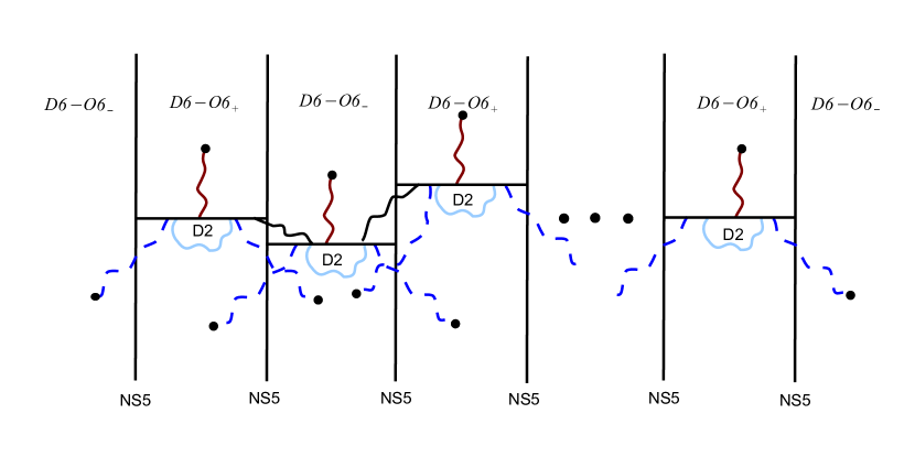
Refer to caption
Figure 3: Type IIA brane setup corresponding to M5 branes probing Dp+4subscript𝐷𝑝4D_{p+4} a singularity. The fundamental strings depicted as blue or red wavy lines in this Figure give rise to fields in the 2d quiver theory.
Refer to caption
Figure 4: Non-critical strings in M5 branes probing Dp+4subscript𝐷𝑝4D_{p+4} singularities.

Having an explicit description of the two-dimensional quiver theory makes it possible to compute the corresponding elliptic genus. In the simplest case of a single tensor multiplet corresponding to a (1)1(-1) curve, this corresponds to the E-string elliptic genus which was studied in detail in Kim:2014dza (although in the present setup one must identify the fugacities associated to the two SO(8)𝑆𝑂8SO(8) subgroups of the SO(16)𝑆𝑂16SO(16) flavor symmetry group). For the sake of illustration, let us also consider the non-Higgsable (1)(4)(1)141(-1)(-4)(-1) theory with three tensor multiplets, gauge group SO(8)g𝑆𝑂subscript8𝑔SO(8)_{g} and flavor group SO(8)L×SO(8)R𝑆𝑂subscript8𝐿𝑆𝑂subscript8𝑅SO(8)_{L}\times SO(8)_{R}. Let us denote by m(g)superscriptsubscript𝑚𝑔m_{\ell}^{(g)}, =1,,414\ell=1,\dots,4 the fugacities associated to SO(8)g𝑆𝑂subscript8𝑔SO(8)_{g} and by m(L)superscriptsubscript𝑚𝐿m_{\ell}^{(L)} (m(R)superscriptsubscript𝑚𝑅m_{\ell}^{(R)}) the ones associated to SO(8)L𝑆𝑂subscript8𝐿SO(8)_{L} (SO(8)R𝑆𝑂subscript8𝑅SO(8)_{R}). From the previous discussion, one can write down the elliptic genus for any bound state of the strings associated to this theory. For instance, if one considers the bound state of one string coupled to the first (1)1(-1) tensor multiplet and one string coupled to the (4)4(-4) multiplet, one finds:

(1)(4)subscript14\displaystyle\mathcal{I}_{(-1)(-4)} =14𝑑uη2i=14(η2θ1(ϵ1)θ1(ϵ2))(=14θi(m(L))η)(=14θi(m(g))η)absent14contour-integraldifferential-d𝑢superscript𝜂2superscriptsubscript𝑖14superscript𝜂2subscript𝜃1subscriptitalic-ϵ1subscript𝜃1subscriptitalic-ϵ2superscriptsubscriptproduct14subscript𝜃𝑖superscriptsubscript𝑚𝐿𝜂superscriptsubscriptproduct14subscript𝜃𝑖superscriptsubscript𝑚𝑔𝜂\displaystyle=\frac{1}{4}\oint du\eta^{2}\sum_{i=1}^{4}\left(\frac{\eta^{2}}{\theta_{1}(\epsilon_{1})\theta_{1}(\epsilon_{2})}\right)\left(\prod_{\ell=1}^{4}\frac{\theta_{i}(m_{\ell}^{(L)})}{\eta}\right)\left(\prod_{\ell=1}^{4}\frac{\theta_{i}(m_{\ell}^{(g)})}{\eta}\right)
×(θ1(2u)2θ1(2ϵ+)θ1(2u+2ϵ+)θ1(2u+2ϵ+)η3θ1(ϵ1)θ1(ϵ2))absentsubscript𝜃1superscript2𝑢2subscript𝜃12subscriptitalic-ϵsubscript𝜃12𝑢2subscriptitalic-ϵsubscript𝜃12𝑢2subscriptitalic-ϵsuperscript𝜂3subscript𝜃1subscriptitalic-ϵ1subscript𝜃1subscriptitalic-ϵ2\displaystyle\times\left(\frac{\theta_{1}(2u)^{2}\theta_{1}(2\epsilon_{+})\theta_{1}(2u+2\epsilon_{+})\theta_{1}(-2u+2\epsilon_{+})}{\eta^{3}\theta_{1}(\epsilon_{1})\theta_{1}(\epsilon_{2})}\right)
×(=14η4θ1(ϵ++m(g)+u)θ1(ϵ++m(g)u)θ1(ϵ+m(g)+u)θ1(ϵ+m(g)u))absentsuperscriptsubscriptproduct14superscript𝜂4subscript𝜃1subscriptitalic-ϵsubscriptsuperscript𝑚𝑔𝑢subscript𝜃1subscriptitalic-ϵsubscriptsuperscript𝑚𝑔𝑢subscript𝜃1subscriptitalic-ϵsubscriptsuperscript𝑚𝑔𝑢subscript𝜃1subscriptitalic-ϵsubscriptsuperscript𝑚𝑔𝑢\displaystyle\times\left(\prod_{\ell=1}^{4}\frac{\eta^{4}}{\theta_{1}(\epsilon_{+}\!+\!m^{(g)}_{\ell}\!+\!u)\theta_{1}(\epsilon_{+}\!+\!m^{(g)}_{\ell}\!-\!u)\theta_{1}(\epsilon_{+}\!-\!m^{(g)}_{\ell}\!+\!u)\theta_{1}(\epsilon_{+}\!-\!m^{(g)}_{\ell}\!-\!u)}\right)
×(θi(ϵu)θi(ϵ+u)θi(ϵ+u)θi(ϵ++u)),absentsubscript𝜃𝑖subscriptitalic-ϵ𝑢subscript𝜃𝑖subscriptitalic-ϵ𝑢subscript𝜃𝑖subscriptitalic-ϵ𝑢subscript𝜃𝑖subscriptitalic-ϵ𝑢\displaystyle\times\left(\frac{\theta_{i}(\epsilon_{-}-u)\theta_{i}(\epsilon_{-}+u)}{\theta_{i}(-\epsilon_{+}-u)\theta_{i}(-\epsilon_{+}+u)}\right), (4)

where

η=q1/24i=1(1qi),q=e2πiτformulae-sequence𝜂superscript𝑞124superscriptsubscriptproduct𝑖11superscript𝑞𝑖𝑞superscript𝑒2𝜋𝑖𝜏\eta=q^{1/24}\prod_{i=1}^{\infty}(1-q^{i}),\qquad q=e^{2\pi i\tau} (5)

and

θ1(x)=iq1/8eπix(1e2πix)i=1(1qi)(1qie2πix)(1qie2πix).subscript𝜃1𝑥𝑖superscript𝑞18superscript𝑒𝜋𝑖𝑥1superscript𝑒2𝜋𝑖𝑥superscriptsubscriptproduct𝑖11superscript𝑞𝑖1superscript𝑞𝑖superscript𝑒2𝜋𝑖𝑥1superscript𝑞𝑖superscript𝑒2𝜋𝑖𝑥\theta_{1}(x)=i\,q^{1/8}e^{-\pi ix}(1-e^{2\pi ix})\prod_{i=1}^{\infty}(1-q^{i})(1-q^{i}e^{2\pi ix})(1-q^{i}e^{-2\pi ix}). (6)

The contour integral can be performed by using the Jeffrey-Kirwan prescription for computing residues Benini:2013xpa . Similarly, one can compute the elliptic genus for other bound states of strings.

4 Multiple M5 branes probing an M9 wall

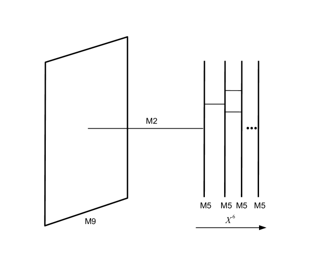
In this section we study the 𝒩=(1,0)𝒩10\mathcal{N}=(1,0) six-dimensional theory of N𝑁N small E8subscript𝐸8E_{8} instantons Ganor:1996mu ; Seiberg:1996vs ; upon moving to the tensor branch, this becomes the theory of N𝑁N parallel M5 branes in the proximity of the M9 boundary wall of M-theory. The strings originate from M2 branes that are suspended between neighboring M5 branes or between the M5 branes and the M9 plane (see Figure 5). Upon circle reduction to five dimensions with an E8subscript𝐸8E_{8} background Wilson line (which breaks E8subscript𝐸8E_{8} global symmetry to SO(16)𝑆𝑂16SO(16)), the theory of N𝑁N small instantons reduces to the Sp(N)𝑆𝑝𝑁Sp(N) theory with 888 fundamental and 111 antisymmetric hypermultiplets Seiberg:1996vs . The instanton calculus for this five-dimensional theory provides a way to check elliptic genus computations and will be exploited in Section 4.2.
Refer to caption
Figure 5: E-strings as suspended M2 branes between M5 branes probing an M9 wall.

4.1 Two-dimensional quiver

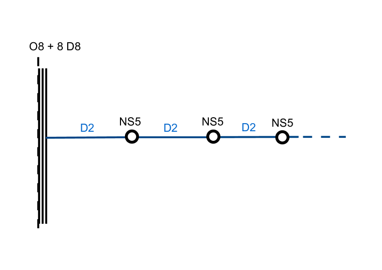
In order to derive a quiver description for the theory of the strings, it again proves useful to switch to an equivalent brane configuration within string theory. Let us begin by discussing N=1𝑁1N=1 theory of a single small E8subscript𝐸8E_{8} instanton, whose associated two-dimensional quiver gauge theory has been worked out in Kim:2014dza . The quiver was derived from a Type I’ brane configuration, which arises as follows: upon reduction of M-theory on a circle, the M9 plane is replaced by eight D8 branes on top of an O8superscript88^{-} orientifold plane (which has D8 brane charge 88-8); the M5 brane, on the other hand, becomes an NS5 brane. Furthermore, M2 branes are replaced by D2 branes that stretch between the NS5 brane and the D8-O8- system. By studying the two-dimensional reduction of the worldvolume theory of the D2 branes in the limit of small separation between the NS5 and eight-branes, one arrives at the two-dimensional quiver gauge theory of Kim:2014dza . The (0,4) quiver gauge theory for n𝑛n strings has gauge group O(n)𝑂𝑛O(n) and the following field content: a vector multiplet in the adjoint (anti-symmetric) representation of O(n)𝑂𝑛O(n), a hypermultiplet in the symmetric representation, and eight Fermi multiplets in the bifundamental representation of O(n)×SO(16)𝑂𝑛𝑆𝑂16O(n)\times SO(16). Elliptic genera for this theory have been computed in Kim:2014dza for up to four strings and shown to agree with results from the instanton calculus for the five-dimensional Sp(1)𝑆𝑝1Sp(1) theory with eight fundamental hypermultiplets.

The generalization of the Type I’ brane setup to the case of N𝑁N small instantons is illustrated in Figure 6 and is again obtained by reducing the above M9-M5 setup on a circle. The brane setup is a combination of the E-string and M-string brane configurations without the D6 branes which are usually present for the M-string system. As we will see this becomes crucial when we look at the quiver-gauge theory governing the dynamics of the strings to which we now turn.
Refer to caption
Figure 6: Brane configuration for the theory of N𝑁N small E8subscript𝐸8E_{8} instantons.

The brane setup implies a simple quiver gauge theory governing the dynamics of the strings. The first n1subscript𝑛1n_{1} D2 branes ending on the D8-O8 system correspond to a O(n1)𝑂subscript𝑛1O(n_{1}) gauge node; from the D2-D8 strings one finds eight bifundamental Fermi multiplets charged under O(n1)×SO(16)𝑂subscript𝑛1𝑆𝑂16O(n_{1})\times SO(16). Furthermore, there is a symmetric hyper at the O(n1)𝑂subscript𝑛1O(n_{1}) node as already observed in Kim:2014dza . All other gauge nodes corresponding to the the D2 branes suspended between NS5 branes have unitary gauge groups with bi-fundamental matter between them familiar from the orbifolds of M-strings Haghighat:2013tka . Finally, one also obtains O(n1)×U(n2)𝑂subscript𝑛1𝑈subscript𝑛2O(n_{1})\times U(n_{2}) bifundamentals from strings ending on the n1subscript𝑛1n_{1} and n2subscript𝑛2n_{2} D2 branes. These bifundamental fields consist of a (0,4) hyper and a (0,4) Fermi multiplet, as is the case for M-strings. The resulting quiver is illustrated in Figure 7.

We comment on the global symmetries of this quiver gauge theory, and compare them with the symmetries that we expect for the infrared CFT on these strings. Our (0,4)04(0,4) gauge theory has SO(4)=SU(2)×SU(2)𝑆𝑂4𝑆𝑈2𝑆𝑈2SO(4)=SU(2)\times SU(2) R-symmetry. The first SU(2)𝑆𝑈2SU(2) is part of the SO(4)𝑆𝑂4SO(4) symmetry which rotates 4superscript4\mathbb{R}^{4} along the worldvolume of NS5-branes, transverse to the strings. The second SU(2)SO(3)similar-to𝑆𝑈2𝑆𝑂3SU(2)\sim SO(3) rotates the 3superscript3\mathbb{R}^{3} space transverse to the NS5-branes and D2-branes. The infrared (or equivalently strong coupling) limit of the 2d gauge theory is realized by going to the M-theory regime of the type I’ theory. Then the space 3superscript3\mathbb{R}^{3} transverse to NS5-D2 is replaced by 3×S1superscript3superscript𝑆1\mathbb{R}^{3}\times S^{1}, including the M-theory circle, and becomes 4superscript4\mathbb{R}^{4} in the strong coupling limit. So in the IR, we expect the SO(3)𝑆𝑂3SO(3) symmetry to enhance to SO(4)𝑆𝑂4SO(4). Any analysis from our gauge theory, such as the elliptic genus calculus below, will be missing the extra Cartan charges of the enhanced SO(4)𝑆𝑂4SO(4). Let us denote by ϵ1,2subscriptitalic-ϵ12\epsilon_{1,2} the chemical potentials for the rotations on 4superscript4\mathbb{R}^{4}, as in the previous sections. Apart from rotating 4superscript4\mathbb{R}^{4} along the 5-brane, there will be an extra rotation on 4superscript4\mathbb{R}^{4} transverse to the M5-brane, with ϵ+ϵ1+ϵ22subscriptitalic-ϵsubscriptitalic-ϵ1subscriptitalic-ϵ22\epsilon_{+}\equiv\frac{\epsilon_{1}+\epsilon_{2}}{2}. Let us denote by m𝑚m the chemical potential for the missing Cartan of the enhanced IR symmetry. Then the 3superscript3\mathbb{R}^{3} part in the type I’ setting is rotated by m+ϵ+𝑚subscriptitalic-ϵm+\epsilon_{+}, while the rotation by mϵ+𝑚subscriptitalic-ϵm-\epsilon_{+} is invisible on 3×S1superscript3superscript𝑆1\mathbb{R}^{3}\times S^{1}. Thus, our UV gauge theory will be computing the elliptic genus only at m=ϵ+𝑚subscriptitalic-ϵm=\epsilon_{+}111The parameter m𝑚m is the one appearing in the instanton calculus of the Nekrasov partition function and should not be confused with the fugacity of U(1)m𝑈subscript1𝑚U(1)_{m} in the 2d gauge theory. With respect to the 2d fugacity it is shifted by ϵ+subscriptitalic-ϵ\epsilon_{+}..

At N=1𝑁1N=1, it is known that the 6d SCFT engineered by a single M5 and M9 brane does not see the extra Cartan of SO(4)𝑆𝑂4SO(4) (conjugate to m𝑚m) at all. In other words, all the states in the Hilbert space of the 6d SCFT are completely neutral under this U(1)𝑈1U(1) charge (while the full M-theory would see the charged states decoupled from the 6d SCFT). One way to see this is from the 5 dimensional Sp(N)𝑆𝑝𝑁Sp(N) gauge theory obtained after circle compactification. Namely, the parameter m𝑚m above corresponds to the mass parameter for the Sp(N)𝑆𝑝𝑁Sp(N) antisymmetric hypermultiplet in the resulting 5d theory. At N=1𝑁1N=1, the antisymmetric representation is neutral in Sp(1)𝑆𝑝1Sp(1) and the corresponding hypermultiplet decouples. This implies that the extra U(1)𝑈1U(1) for m𝑚m decouples from the 6d CFT at N=1𝑁1N=1, and this has been tested from the instanton partition function in Hwang:2014uwa . This is the reason why the 2d gauge theory above provided maximally refined elliptic genera at N=1𝑁1N=1 in Kim:2014dza , since the restriction m=ϵ+𝑚subscriptitalic-ϵm=\epsilon_{+} loses no information about the 6d SCFT. However, the parameter m𝑚m appears in the 6d CFT spectrum for N2𝑁2N\geq 2, which was checked from the Sp(N)𝑆𝑝𝑁Sp(N) instanton calculus Hwang:2014uwa .

Below we present sample computations for the elliptic genera corresponding to the lowest charge sectors, namely (n1,n2)=(1,1)subscript𝑛1subscript𝑛211(n_{1},n_{2})=(1,1), (n1,n2)=(1,2)subscript𝑛1subscript𝑛212(n_{1},n_{2})=(1,2), and (n1,n2)=(2,1)subscript𝑛1subscript𝑛221(n_{1},n_{2})=(2,1) for the N=2𝑁2N=2 quiver.

Refer to caption
Figure 7: Quiver for the theory of N𝑁N small E8subscript𝐸8E_{8} instantons.

Charge sector (n1,n2)=(1,1)subscript𝑛1subscript𝑛211(n_{1},n_{2})=(1,1)

Combining the one-loop determinants, the zero-mode integral I(1,1)subscript𝐼11I_{(1,1)} is given by

du2i=14(η2θ1(ϵ1)θ1(ϵ2))1(η3θ1(ϵ1+ϵ2)θ1(ϵ1)θ1(ϵ2))2(l=18θ1(ml+ai)η)3(θ1(+ϵ±(aiu))θ1(ϵ+±(aiu)))4contour-integral𝑑𝑢2superscriptsubscript𝑖14subscriptsuperscript𝜂2subscript𝜃1subscriptitalic-ϵ1subscript𝜃1subscriptitalic-ϵ21subscriptsuperscript𝜂3subscript𝜃1subscriptitalic-ϵ1subscriptitalic-ϵ2subscript𝜃1subscriptitalic-ϵ1subscript𝜃1subscriptitalic-ϵ22subscriptsuperscriptsubscriptproduct𝑙18subscript𝜃1subscript𝑚𝑙subscript𝑎𝑖𝜂3subscriptsubscript𝜃1plus-or-minussubscriptitalic-ϵsubscript𝑎𝑖𝑢subscript𝜃1plus-or-minussubscriptitalic-ϵsubscript𝑎𝑖𝑢4\displaystyle-\oint\frac{du}{2}\sum_{i=1}^{4}\Bigg{(}\frac{\eta^{2}}{\theta_{1}(\epsilon_{1})\theta_{1}(\epsilon_{2})}\Bigg{)}_{1}\!\Bigg{(}\frac{\eta^{3}\theta_{1}(\epsilon_{1}\!+\!\epsilon_{2})}{\theta_{1}(\epsilon_{1})\theta_{1}(\epsilon_{2})}\Bigg{)}_{2}\!\Bigg{(}\prod_{l=1}^{8}\frac{\theta_{1}(m_{l}\!+\!a_{i})}{\eta}\Bigg{)}_{3}\!\Bigg{(}\frac{\theta_{1}(+\epsilon_{-}\!\pm\!(a_{i}\!-\!u))}{\theta_{1}(-\epsilon_{+}\!\pm\!(a_{i}\!-\!u))}\Bigg{)}_{4} (7)

where ai=(0,12,1+τ2,τ2)isubscript𝑎𝑖subscript0121𝜏2𝜏2𝑖a_{i}=(0,\frac{1}{2},\frac{1+\tau}{2},\frac{\tau}{2})_{i}. Repeated signs ±plus-or-minus\pm in the arguments mean that both factors are multiplied: θ1(ϵ+±(aiu))θ1(ϵ++aiu)θ1(ϵ+ai+u)subscript𝜃1plus-or-minussubscriptitalic-ϵsubscript𝑎𝑖𝑢subscript𝜃1subscriptitalic-ϵsubscript𝑎𝑖𝑢subscript𝜃1subscriptitalic-ϵsubscript𝑎𝑖𝑢\theta_{1}(-\epsilon_{+}\pm(a_{i}-u))\equiv\theta_{1}(-\epsilon_{+}+a_{i}-u)\theta_{1}(-\epsilon_{+}-a_{i}+u). The contour integral given by the JK-Res is done with η=e1𝜂subscript𝑒1\eta=e_{1}. Then the only nonzero JK-Res comes from the pole u=ai+ϵ+𝑢subscript𝑎𝑖subscriptitalic-ϵu=a_{i}+\epsilon_{+}. The result is

I(1,1)=subscript𝐼11absent\displaystyle I_{(1,1)}= η5θ1(ϵ1+ϵ2)2θ1(ϵ1)2θ1(ϵ2)2i=14(l=18θ1(ml+ai)η)θ1(ϵ1)θ1(ϵ2)η3θ1(ϵ1ϵ2)superscript𝜂5subscript𝜃1subscriptitalic-ϵ1subscriptitalic-ϵ22subscript𝜃1superscriptsubscriptitalic-ϵ12subscript𝜃1superscriptsubscriptitalic-ϵ22superscriptsubscript𝑖14superscriptsubscriptproduct𝑙18subscript𝜃1subscript𝑚𝑙subscript𝑎𝑖𝜂subscript𝜃1subscriptitalic-ϵ1subscript𝜃1subscriptitalic-ϵ2superscript𝜂3subscript𝜃1subscriptitalic-ϵ1subscriptitalic-ϵ2\displaystyle-\frac{\eta^{5}\theta_{1}(\epsilon_{1}+\epsilon_{2})}{2\theta_{1}(\epsilon_{1})^{2}\theta_{1}(\epsilon_{2})^{2}}\sum_{i=1}^{4}\Bigg{(}\prod_{l=1}^{8}\frac{\theta_{1}(m_{l}+a_{i})}{\eta}\Bigg{)}\frac{\theta_{1}(\epsilon_{1})\theta_{1}(-\epsilon_{2})}{\eta^{3}\theta_{1}(-\epsilon_{1}-\epsilon_{2})} (8)
=\displaystyle= η22θ1(ϵ1)θ1(ϵ2)i=14(l=18θi(ml)η)=I(1,0).superscript𝜂22subscript𝜃1subscriptitalic-ϵ1subscript𝜃1subscriptitalic-ϵ2superscriptsubscript𝑖14superscriptsubscriptproduct𝑙18subscript𝜃𝑖subscript𝑚𝑙𝜂subscript𝐼10\displaystyle-\frac{\eta^{2}}{2\theta_{1}(\epsilon_{1})\theta_{1}(\epsilon_{2})}\sum_{i=1}^{4}\Bigg{(}\prod_{l=1}^{8}\frac{\theta_{i}(m_{l})}{\eta}\Bigg{)}=I_{(1,0)}\ .

This is the elliptic genus of the single E-string, i.e. with charge (n1,n2)=(1,0)subscript𝑛1subscript𝑛210(n_{1},n_{2})=(1,0) Klemm:1996hh ; Kim:2014dza .

Charge sector (n1,n2)=(1,2)subscript𝑛1subscript𝑛212(n_{1},n_{2})=(1,2)

The zero-mode integral is given by

I(1,2)=subscript𝐼12absent\displaystyle I_{(1,2)}= du1du24i=14η2θ1(ϵ1)θ1(ϵ2)(η3θ1(ϵ1+ϵ2)θ1(ϵ1)θ1(ϵ2))2(l=18θ1(ml+ai)η)contour-integral𝑑subscript𝑢1𝑑subscript𝑢24superscriptsubscript𝑖14superscript𝜂2subscript𝜃1subscriptitalic-ϵ1subscript𝜃1subscriptitalic-ϵ2superscriptsuperscript𝜂3subscript𝜃1subscriptitalic-ϵ1subscriptitalic-ϵ2subscript𝜃1subscriptitalic-ϵ1subscript𝜃1subscriptitalic-ϵ22superscriptsubscriptproduct𝑙18subscript𝜃1subscript𝑚𝑙subscript𝑎𝑖𝜂\displaystyle-\oint\frac{du_{1}du_{2}}{4}\;\sum_{i=1}^{4}\frac{\eta^{2}}{\theta_{1}(\epsilon_{1})\theta_{1}(\epsilon_{2})}\Bigg{(}\frac{\eta^{3}\theta_{1}(\epsilon_{1}+\epsilon_{2})}{\theta_{1}(\epsilon_{1})\theta_{1}(\epsilon_{2})}\Bigg{)}^{2}\Bigg{(}\prod_{l=1}^{8}\frac{\theta_{1}(m_{l}+a_{i})}{\eta}\Bigg{)}
×θ1(±(u1u2))θ1(ϵ1+ϵ2±(u1u2))θ1(ϵ1±(u1u2))θ1(ϵ2±(u1u2))θ1(+ϵ±aiu1)θ1(ϵ+±(aiu1))θ1(+ϵ±aiu2)θ1(ϵ+±aiu2).absentsubscript𝜃1plus-or-minussubscript𝑢1subscript𝑢2subscript𝜃1plus-or-minussubscriptitalic-ϵ1subscriptitalic-ϵ2subscript𝑢1subscript𝑢2subscript𝜃1plus-or-minussubscriptitalic-ϵ1subscript𝑢1subscript𝑢2subscript𝜃1plus-or-minussubscriptitalic-ϵ2subscript𝑢1subscript𝑢2subscript𝜃1minus-or-plusplus-or-minussubscriptitalic-ϵsubscript𝑎𝑖subscript𝑢1subscript𝜃1plus-or-minussubscriptitalic-ϵsubscript𝑎𝑖subscript𝑢1subscript𝜃1minus-or-plusplus-or-minussubscriptitalic-ϵsubscript𝑎𝑖subscript𝑢2subscript𝜃1minus-or-plusplus-or-minussubscriptitalic-ϵsubscript𝑎𝑖subscript𝑢2\displaystyle\times\frac{\theta_{1}(\pm(u_{1}\!-\!u_{2}))\theta_{1}(\epsilon_{1}\!+\!\epsilon_{2}\!\pm\!(u_{1}\!-\!u_{2}))}{\theta_{1}(\epsilon_{1}\!\pm\!(u_{1}\!-\!u_{2}))\theta_{1}(\epsilon_{2}\!\pm\!(u_{1}\!-\!u_{2}))}\frac{\theta_{1}(+\epsilon_{-}\!\pm\!a_{i}\!\mp\!u_{1})}{\theta_{1}(-\epsilon_{+}\!\pm\!(a_{i}\!-\!u_{1}))}\frac{\theta_{1}(+\epsilon_{-}\!\pm\!a_{i}\!\mp\!u_{2})}{\theta_{1}(-\epsilon_{+}\!\pm\!a_{i}\!\mp\!u_{2})}. (9)

If we choose η=e1+ϵe2𝜂subscript𝑒1italic-ϵsubscript𝑒2\eta=e_{1}+\epsilon\,e_{2} in which ϵ1much-less-thanitalic-ϵ1\epsilon\ll 1, nonzero JK-Res can only come from the following poles.

  • (ϵ1,2u1+u2,ϵ+ai+u1)=(0,0)subscriptitalic-ϵ12subscript𝑢1subscript𝑢2subscriptitalic-ϵsubscript𝑎𝑖subscript𝑢100(\epsilon_{1,2}-u_{1}+u_{2},-\epsilon_{+}-a_{i}+u_{1})=(0,0)

  • (ϵ1,2+u1u2,ϵ+ai+u2)=(0,0)subscriptitalic-ϵ12subscript𝑢1subscript𝑢2subscriptitalic-ϵsubscript𝑎𝑖subscript𝑢200(\epsilon_{1,2}+u_{1}-u_{2},-\epsilon_{+}-a_{i}+u_{2})=(0,0)

  • (ϵ+ai+u1,ϵ+ai+u2)=(0,0)subscriptitalic-ϵsubscript𝑎𝑖subscript𝑢1subscriptitalic-ϵsubscript𝑎𝑖subscript𝑢200(-\epsilon_{+}-a_{i}+u_{1},-\epsilon_{+}-a_{i}+u_{2})=(0,0).

Actually evaluating the residues, it turns out that all these poles yield vanishing residues, so that

I(1,2)=subscript𝐼12absent\displaystyle I_{(1,2)}= 0.0\displaystyle 0. (10)

Charge sector (n1,n2)=(2,1)subscript𝑛1subscript𝑛221(n_{1},n_{2})=(2,1)

Now the gauge theory comes with O(2)×U(1)𝑂2𝑈1O(2)\times U(1) gauge group. In the elliptic genus calculus, there are seven disconnected sectors of O(2)𝑂2O(2) flat connections Kim:2014dza . In six sectors, the flat connections are discrete, while in one sector it comes with one complex parameter.

In the first sector with continuous parameter, which we label by superscript 00, one has to do the following rank 222 contour integral for the elliptic genus:

I(2,1)0=superscriptsubscript𝐼210absent\displaystyle I_{(2,1)}^{0}= du1du22η7θ1(ϵ1+ϵ2)θ1(ϵ1,2)θ1(ϵ1,2±2u1)η3θ1(ϵ1+ϵ2)θ1(ϵ1)θ1(ϵ2)(l=18θ1(ml±u1)η2)contour-integral𝑑subscript𝑢1𝑑subscript𝑢22superscript𝜂7subscript𝜃1subscriptitalic-ϵ1subscriptitalic-ϵ2subscript𝜃1subscriptitalic-ϵ12subscript𝜃1plus-or-minussubscriptitalic-ϵ122subscript𝑢1superscript𝜂3subscript𝜃1subscriptitalic-ϵ1subscriptitalic-ϵ2subscript𝜃1subscriptitalic-ϵ1subscript𝜃1subscriptitalic-ϵ2superscriptsubscriptproduct𝑙18subscript𝜃1plus-or-minussubscript𝑚𝑙subscript𝑢1superscript𝜂2\displaystyle\oint\frac{du_{1}du_{2}}{2}\;\frac{\eta^{7}\theta_{1}(\epsilon_{1}+\epsilon_{2})}{\theta_{1}(\epsilon_{1,2})\theta_{1}(\epsilon_{1,2}\pm 2u_{1})}\frac{\eta^{3}\theta_{1}(\epsilon_{1}+\epsilon_{2})}{\theta_{1}(\epsilon_{1})\theta_{1}(\epsilon_{2})}\Bigg{(}\prod_{l=1}^{8}\frac{\theta_{1}(m_{l}\pm u_{1})}{\eta^{2}}\Bigg{)} (11)
×θ1(+ϵ±u1+u2)θ1(ϵ+±u1+u2)θ1(+ϵ±u1u2)θ1(ϵ+±u1u2)absentsubscript𝜃1plus-or-minussubscriptitalic-ϵsubscript𝑢1subscript𝑢2subscript𝜃1plus-or-minussubscriptitalic-ϵsubscript𝑢1subscript𝑢2subscript𝜃1plus-or-minussubscriptitalic-ϵsubscript𝑢1subscript𝑢2subscript𝜃1plus-or-minussubscriptitalic-ϵsubscript𝑢1subscript𝑢2\displaystyle\times\frac{\theta_{1}(+\epsilon_{-}\pm u_{1}+u_{2})}{\theta_{1}(-\epsilon_{+}\pm u_{1}+u_{2})}\frac{\theta_{1}(+\epsilon_{-}\pm u_{1}-u_{2})}{\theta_{1}(-\epsilon_{+}\pm u_{1}-u_{2})}

If we choose η=e1+ϵe2𝜂subscript𝑒1italic-ϵsubscript𝑒2\eta=e_{1}+\epsilon\,e_{2} in which ϵ1much-less-thanitalic-ϵ1\epsilon\ll 1, nonzero JK-res can only appear from the following poles.

  • (ϵ+u1+u2,ϵ1,2+2u1)=(0,0)(u1,u2)=(ϵ1,22+ai,ϵ2,12+ai)subscriptitalic-ϵsubscript𝑢1subscript𝑢2subscriptitalic-ϵ122subscript𝑢100subscript𝑢1subscript𝑢2subscriptitalic-ϵ122subscript𝑎𝑖subscriptitalic-ϵ212subscript𝑎𝑖(-\epsilon_{+}-u_{1}+u_{2},\epsilon_{1,2}+2u_{1})=(0,0)\longrightarrow(u_{1},u_{2})=(-\tfrac{\epsilon_{1,2}}{2}+a_{i},\tfrac{\epsilon_{2,1}}{2}+a_{i}). Its residue is zero.

  • (ϵ++u1u2,ϵ++u1+u2)=(0,0)(u1,u2)=(ϵ++ai,ai)subscriptitalic-ϵsubscript𝑢1subscript𝑢2subscriptitalic-ϵsubscript𝑢1subscript𝑢200subscript𝑢1subscript𝑢2subscriptitalic-ϵsubscript𝑎𝑖subscript𝑎𝑖(-\epsilon_{+}+u_{1}-u_{2},-\epsilon_{+}+u_{1}+u_{2})=(0,0)\longrightarrow(u_{1},u_{2})=(\epsilon_{+}+a_{i},a_{i})

  • (ϵ++u1+u2,ϵ1,2+2u1)=(0,0)(u1,u2)=(ϵ1,22+ai,ϵ1,2+ϵ2,12ai)subscriptitalic-ϵsubscript𝑢1subscript𝑢2subscriptitalic-ϵ122subscript𝑢100subscript𝑢1subscript𝑢2subscriptitalic-ϵ122subscript𝑎𝑖subscriptitalic-ϵ12subscriptitalic-ϵ212subscript𝑎𝑖(-\epsilon_{+}+u_{1}+u_{2},\epsilon_{1,2}+2u_{1})=(0,0)\longrightarrow(u_{1},u_{2})=(-\tfrac{\epsilon_{1,2}}{2}+a_{i},\epsilon_{1,2}+\tfrac{\epsilon_{2,1}}{2}-a_{i})

Collecting all the residues, I(2,1)0superscriptsubscript𝐼210I_{(2,1)}^{0} is given by

I(2,1)0superscriptsubscript𝐼210\displaystyle I_{(2,1)}^{0} =η124θ1(ϵ1)θ1(ϵ2)i=14[l=18θi(ml±ϵ+)θ1(2ϵ1+ϵ2)θ1(ϵ1+2ϵ2)\displaystyle=\frac{\eta^{-12}}{4\theta_{1}(\epsilon_{1})\theta_{1}(\epsilon_{2})}\sum_{i=1}^{4}\Bigg{[}\frac{\prod_{l=1}^{8}\theta_{i}(m_{l}\pm\epsilon_{+})}{\theta_{1}(2\epsilon_{1}+\epsilon_{2})\theta_{1}(\epsilon_{1}+2\epsilon_{2})}
(θ1(ϵ1+ϵ2)l=18θi(ml±ϵ12)θ1(ϵ1)θ1(ϵ1ϵ2)θ1(2ϵ1+ϵ2)+(ϵ1ϵ2))]\displaystyle\hskip 108.405pt-\Bigg{(}\frac{\theta_{1}(\epsilon_{1}+\epsilon_{2})\prod_{l=1}^{8}\theta_{i}(m_{l}\pm\tfrac{\epsilon_{1}}{2})}{\theta_{1}(\epsilon_{1})\theta_{1}(\epsilon_{1}-\epsilon_{2})\theta_{1}(2\epsilon_{1}+\epsilon_{2})}+(\epsilon_{1}\leftrightarrow\epsilon_{2})\Bigg{)}\Bigg{]}
=η44θ1(ϵ1)2θ1(ϵ2)2i=14(l=18θi(ml)2η2).absentsuperscript𝜂44subscript𝜃1superscriptsubscriptitalic-ϵ12subscript𝜃1superscriptsubscriptitalic-ϵ22superscriptsubscript𝑖14superscriptsubscriptproduct𝑙18subscript𝜃𝑖superscriptsubscript𝑚𝑙2superscript𝜂2\displaystyle=\frac{\eta^{4}}{4\theta_{1}(\epsilon_{1})^{2}\theta_{1}(\epsilon_{2})^{2}}\sum_{i=1}^{4}\Bigg{(}\prod_{l=1}^{8}\frac{\theta_{i}(m_{l})^{2}}{\eta^{2}}\Bigg{)}\ . (12)

On the second line, we used the following identity

i=14superscriptsubscript𝑖14\displaystyle\sum_{i=1}^{4} l=18θi(ml)2=i=14[θ1(ϵ1,2)l=18θi(ml±ϵ+)θ1(2ϵ1+ϵ2)θ1(ϵ1+2ϵ2)\displaystyle\prod_{l=1}^{8}\theta_{i}(m_{l})^{2}=\sum_{i=1}^{4}\,\,\!\!\Bigg{[}\frac{\theta_{1}(\epsilon_{1,2})\prod_{l=1}^{8}\theta_{i}(m_{l}\pm\epsilon_{+})}{\theta_{1}(2\epsilon_{1}+\epsilon_{2})\theta_{1}(\epsilon_{1}+2\epsilon_{2})}
(θ1(ϵ2)θ1(ϵ1+ϵ2)l=18θi(ml±ϵ12)θ1(2ϵ1+ϵ2)θ1(ϵ1ϵ2)+(ϵ1ϵ2))],\displaystyle\hskip 97.56493pt-\Bigg{(}\frac{\theta_{1}(\epsilon_{2})\theta_{1}(\epsilon_{1}+\epsilon_{2})\prod_{l=1}^{8}\theta_{i}(m_{l}\pm\frac{\epsilon_{1}}{2})}{\theta_{1}(2\epsilon_{1}+\epsilon_{2})\theta_{1}(\epsilon_{1}-\epsilon_{2})}+(\epsilon_{1}\leftrightarrow\epsilon_{2})\Bigg{)}\Bigg{]},

which we checked in an expansion in e2πiτsuperscript𝑒2𝜋𝑖𝜏e^{2\pi i\tau}, for the first 555 terms up to (e2πiτ)5/2superscriptsuperscript𝑒2𝜋𝑖𝜏52(e^{2\pi i\tau})^{5/2} order.

The contributions from the other six sectors are given by

I(2,1)msuperscriptsubscript𝐼21𝑚\displaystyle I_{(2,1)}^{m} =du4η4θ1(a1+a2)θ1(ϵ1+ϵ2+a1+a2)θ1(ϵ1,2)2θ1(ϵ1,2+a1+a2)η3θ1(ϵ1+ϵ2)θ1(ϵ1)θ1(ϵ2)absentcontour-integral𝑑𝑢4superscript𝜂4subscript𝜃1subscript𝑎1subscript𝑎2subscript𝜃1subscriptitalic-ϵ1subscriptitalic-ϵ2subscript𝑎1subscript𝑎2subscript𝜃1superscriptsubscriptitalic-ϵ122subscript𝜃1subscriptitalic-ϵ12subscript𝑎1subscript𝑎2superscript𝜂3subscript𝜃1subscriptitalic-ϵ1subscriptitalic-ϵ2subscript𝜃1subscriptitalic-ϵ1subscript𝜃1subscriptitalic-ϵ2\displaystyle=\oint\frac{du}{4}\frac{\eta^{4}\theta_{1}(a_{1}+a_{2})\theta_{1}(\epsilon_{1}+\epsilon_{2}+a_{1}+a_{2})}{\theta_{1}(\epsilon_{1,2})^{2}\theta_{1}(\epsilon_{1,2}+a_{1}+a_{2})}\frac{\eta^{3}\theta_{1}(\epsilon_{1}+\epsilon_{2})}{\theta_{1}(\epsilon_{1})\theta_{1}(\epsilon_{2})}
×(l=18θ1(ml+a1)θ1(ml+a2)η2)θ1(+ϵ±a1u)θ1(ϵ+±a1u)θ1(+ϵ±a2u)θ1(ϵ+±a2u),absentsuperscriptsubscriptproduct𝑙18subscript𝜃1subscript𝑚𝑙subscript𝑎1subscript𝜃1subscript𝑚𝑙subscript𝑎2superscript𝜂2subscript𝜃1minus-or-plusplus-or-minussubscriptitalic-ϵsubscript𝑎1𝑢subscript𝜃1minus-or-plusplus-or-minussubscriptitalic-ϵsubscript𝑎1𝑢subscript𝜃1minus-or-plusplus-or-minussubscriptitalic-ϵsubscript𝑎2𝑢subscript𝜃1minus-or-plusplus-or-minussubscriptitalic-ϵsubscript𝑎2𝑢\displaystyle\times\Bigg{(}\prod_{l=1}^{8}\frac{\theta_{1}(m_{l}+a_{1})\theta_{1}(m_{l}+a_{2})}{\eta^{2}}\Bigg{)}\frac{\theta_{1}(+\epsilon_{-}\pm a_{1}\mp u)}{\theta_{1}(-\epsilon_{+}\pm a_{1}\mp u)}\frac{\theta_{1}(+\epsilon_{-}\pm a_{2}\mp u)}{\theta_{1}(-\epsilon_{+}\pm a_{2}\mp u)}, (13)

where we take the discrete O(2)𝑂2O(2) holonomies (a1,a2)=(0,12)subscript𝑎1subscript𝑎2012(a_{1},a_{2})=(0,\frac{1}{2}), (τ2,1+τ2)𝜏21𝜏2(\frac{\tau}{2},\frac{1+\tau}{2}), (0,τ2)0𝜏2(0,\frac{\tau}{2}), (12,1+τ2)121𝜏2(\frac{1}{2},\frac{1+\tau}{2}), (0,1+τ2)01𝜏2(0,\frac{1+\tau}{2}), (12,τ2)12𝜏2(\frac{1}{2},\frac{\tau}{2}) for m=1,2,,6𝑚126m=1,2,\ \cdots,6, respectively. JK-res with η=e1𝜂subscript𝑒1\eta=e_{1} can be nonzero only at the pole u=a1+ϵ+𝑢subscript𝑎1subscriptitalic-ϵu=a_{1}+\epsilon_{+} or u=a2+ϵ+𝑢subscript𝑎2subscriptitalic-ϵu=a_{2}+\epsilon_{+}, yielding the following result:

I(2,1)msuperscriptsubscript𝐼21𝑚\displaystyle I_{(2,1)}^{m} =η42θ1(ϵ1,2)2l=18θi(ml)θj(ml)η2absentsuperscript𝜂42subscript𝜃1superscriptsubscriptitalic-ϵ122superscriptsubscriptproduct𝑙18subscript𝜃𝑖subscript𝑚𝑙subscript𝜃𝑗subscript𝑚𝑙superscript𝜂2\displaystyle=\frac{\eta^{4}}{2\theta_{1}(\epsilon_{1,2})^{2}}\prod_{l=1}^{8}\frac{\theta_{i}(m_{l})\theta_{j}(m_{l})}{\eta^{2}} (14)

where (i,j)=(1,2),(4,3),(1,4),(2,3),(1,3),(2,4)𝑖𝑗124314231324(i,j)=(1,2),(4,3),(1,4),(2,3),(1,3),(2,4) for m=1,2,,6𝑚126m=1,2,\ \cdots,6. Combining (11) and (14), one obtains

I(2,1)=I(2,1)0+m=16I(2,1)m=(I(1,1))2=(I(1,0))2,subscript𝐼21superscriptsubscript𝐼210superscriptsubscript𝑚16superscriptsubscript𝐼21𝑚superscriptsubscript𝐼112superscriptsubscript𝐼102\displaystyle I_{(2,1)}=I_{(2,1)}^{0}+\sum_{m=1}^{6}I_{(2,1)}^{m}=\left(I_{(1,1)}\right)^{2}=\left(I_{(1,0)}\right)^{2}\ , (15)

which exhibits a factorization structure.


In the next subsection, we will show that all the results above are in complete agreement with the 5 dimensional Sp(2)𝑆𝑝2Sp(2) instanton calculus of Hwang:2014uwa . Before that, let us first try to interpret these rather simple results that we have found at m=ϵ+𝑚subscriptitalic-ϵm=\epsilon_{+}.

The strings made of n1subscript𝑛1n_{1} and n2subscript𝑛2n_{2} D2-branes in Fig. 6, winding a circle, contribute to the elliptic genus as both n1+n2subscript𝑛1subscript𝑛2n_{1}+n_{2} multi-particle states, and also through various threshold bound states with lower particle numbers. There could be various kinds of bound states. Generally, m1(n1)annotatedsubscript𝑚1absentsubscript𝑛1m_{1}(\leq n_{1}) of the n1subscript𝑛1n_{1} strings and m2(n2)annotatedsubscript𝑚2absentsubscript𝑛2m_{2}(\leq n_{2}) of the n2subscript𝑛2n_{2} strings may form bounds. One can first deduce that the index is zero at m=ϵ+𝑚subscriptitalic-ϵm=\epsilon_{+} in the sector which contains bound states with charges (0,m2)0subscript𝑚2(0,m_{2}). This is because the (0,m2)0subscript𝑚2(0,m_{2}) bounds are basically M-strings in a maximally supersymmetric theory. Note that the M-strings are half-BPS states of the 6d (2,0)20(2,0) theory, so will see 888 broken supercharges as Goldstone fermions. This is in contrast to the strings in 6d QFTs preserving (1,0)10(1,0) SUSY only. The extra fermionic zero modes for M-strings provide the factor

sinπ(m+ϵ+)sinπ(mϵ+)𝜋𝑚subscriptitalic-ϵ𝜋𝑚subscriptitalic-ϵ\sin\pi(m+\epsilon_{+})\sin\pi(m-\epsilon_{+}) (16)

to the elliptic genus Kim:2011mv . Thus, M-strings which are unbound to E-strings (i.e. at m1=0subscript𝑚10m_{1}=0) will contribute a 00 factor to the elliptic genus at m=±ϵ±𝑚plus-or-minussubscriptitalic-ϵplus-or-minusm=\pm\epsilon_{\pm}.

With this understood, let us start by considering the sector with (n1,n2)=(1,1)subscript𝑛1subscript𝑛211(n_{1},n_{2})=(1,1). At m=ϵ+𝑚subscriptitalic-ϵm=\epsilon_{+}, there is no contribution from the two particle states (1,0)+(0,1)1001(1,0)+(0,1) due to the above reasoning. So one should only obtain a single particle contribution in the (1,1)11(1,1) sector. This is consistent with our finding I(1,1)=I(1,0)subscript𝐼11subscript𝐼10I_{(1,1)}=I_{(1,0)}. A slightly surprising fact from our finding is that the single particle bound with charges (1,1)11(1,1) behaves exactly the same as a single E-string with charge (1,0)10(1,0), at least at m=ϵ+𝑚subscriptitalic-ϵm=\epsilon_{+}. Although the (1,1)11(1,1) bound look like one long E-string suspended between the M9-plane and the second M5-brane, it penetrates through the first M5-brane so in principle there could be extra contributions to the BPS degeneracies from the intersection. For instance, in the case of M-strings, it is known that the charge (1,0)10(1,0) M-string and the single particle bound part of the (1,1)11(1,1) M-string exhibit different spectra (at general chemical potentials, with mϵ+𝑚subscriptitalic-ϵm\neq\epsilon_{+}) Kim:2011mv . So we interpret that I(1,1)=I(1,0)subscript𝐼11subscript𝐼10I_{(1,1)}=I_{(1,0)} implies some simplification of the (1,1)11(1,1) elliptic genus at m=ϵ+𝑚subscriptitalic-ϵm=\epsilon_{+}.

Other results also have nontrivial implications on the E-/M-string bound state elliptic genera at m=ϵ+𝑚subscriptitalic-ϵm=\epsilon_{+}. For (n1,n2)=(1,2)subscript𝑛1subscript𝑛212(n_{1},n_{2})=(1,2), I(1,2)=0subscript𝐼120I_{(1,2)}=0 implies that there are no (1,2)12(1,2) bound states captured by the elliptic genus at m=ϵ+𝑚subscriptitalic-ϵm=\epsilon_{+}, since we know that (1,1)+(0,1)1101(1,1)+(0,1), (1,0)+(0,2)1002(1,0)+(0,2), or (1,0)+2(0,1)10201(1,0)+2(0,1) multi-particles cannot contribute to the elliptic genus at m=ϵ+𝑚subscriptitalic-ϵm=\epsilon_{+}. As we will consider from the 5d Sp(2)𝑆𝑝2Sp(2) instanton calculus, this feature generalizes to higher string numbers: the (m1,m2)subscript𝑚1subscript𝑚2(m_{1},m_{2}) bounds with m1<m2subscript𝑚1subscript𝑚2m_{1}<m_{2} do not contribute to the elliptic genus at m=ϵ+𝑚subscriptitalic-ϵm=\epsilon_{+}.

Finally, I(2,1)=I(1,0)2subscript𝐼21superscriptsubscript𝐼102I_{(2,1)}=I_{(1,0)}^{2} can also be understood with the above observations. Namely, with a (0,m2)0subscript𝑚2(0,m_{2}) particle yielding a factor of zero in the elliptic genus, the nonzero contribution can come from (1,1)+(1,0)1110(1,1)+(1,0) two particle states. But since we already know that these contributions give equal elliptic genera namely that of a single E-string, we can naturally understand this relation. (So our finding implies that the (2,1)21(2,1) bound does not contribute to the index at m=ϵ+𝑚subscriptitalic-ϵm=\epsilon_{+}.)

Based on the above observations, we propose that

I(n1,n2)subscript𝐼subscript𝑛1subscript𝑛2\displaystyle I_{(n_{1},n_{2})} =\displaystyle= 0ifn1<n20ifsubscript𝑛1subscript𝑛2\displaystyle 0\ \ {\rm if}\ \ n_{1}<n_{2}
=\displaystyle= I(n2,0)I(n1n2,0)ifn1n2.subscript𝐼subscript𝑛20subscript𝐼subscript𝑛1subscript𝑛20ifsubscript𝑛1subscript𝑛2\displaystyle I_{(n_{2},0)}I_{(n_{1}-n_{2},0)}\ \ {\rm if}\ \ n_{1}\geq n_{2}\ .

Namely, at m=ϵ+𝑚subscriptitalic-ϵm=\epsilon_{+}, the (n1,n2)subscript𝑛1subscript𝑛2(n_{1},n_{2}) string elliptic genus factorizes to two E-string elliptic genera. Although we have shown this result for only a few charges from the 2d gauge theories, we shall confirm such factorizations to a much higher order in n1,n2subscript𝑛1subscript𝑛2n_{1},n_{2} from the 5d Sp(2)𝑆𝑝2Sp(2) instanton calculus below.

4.2 Five dimensional Sp(2)𝑆𝑝2Sp(2) instanton calculus

In this subsection, we shall consider the circle compactification of the (1,0)10(1,0) theory on 222 M5 and one M9, and consider the string spectra from the instanton calculus of the resulting 5d gauge theory.

Let us consider the six-dimensional conformal field theory living on two M5 branes probing the M9 plane. The space transverse to the two M5-branes is 4×+superscript4superscript\mathbb{R}^{4}\times\mathbb{R}^{+}, where the latter +superscript\mathbb{R}^{+} is obtained by the 2subscript2\mathbb{Z}_{2} action of M9. This space has SO(4)=SU(2)×SU(2)𝑆𝑂4𝑆𝑈2𝑆𝑈2SO(4)=SU(2)\times SU(2) symmetry. The first SU(2)𝑆𝑈2SU(2) is the superconformal R-symmetry, and the second SU(2)𝑆𝑈2SU(2) is a flavor symmetry. The full flavor symmetry is thus SU(2)×E8𝑆𝑈2subscript𝐸8SU(2)\times E_{8}.

We compactify this system on a circle, with an E8subscript𝐸8E_{8} Wilson line which breaks E8subscript𝐸8E_{8} into SO(16)𝑆𝑂16SO(16). Then at low energy, one obtains a 5 dimensional 𝒩=1𝒩1\mathcal{N}=1 Sp(N)𝑆𝑝𝑁Sp(N) gauge theory with Nf=8subscript𝑁𝑓8N_{f}=8 fundamental and one anti-symmetric hypermultiplet. The 888 masses m~isubscript~𝑚𝑖\tilde{m}_{i} for the fundamental hypermultiplets and the mass m𝑚m for the antisymmetric hypermultiplet are in 1-1 correspondence to the chemical potentials of the E8×SU(2)subscript𝐸8𝑆𝑈2E_{8}\times SU(2) flavor symmetries. The precise relations that we use are given in Hwang:2014uwa ; Kim:2014dza . m𝑚m is simply uplifting to the SU(2)𝑆𝑈2SU(2) flavor chemical potential, while the masses m~isubscript~𝑚𝑖\tilde{m}_{i} are related to the E8subscript𝐸8E_{8} chemical potentials misubscript𝑚𝑖m_{i} by Kim:2014dza

m~i=mi(fori=1,,7),m~8=m8τ.formulae-sequencesubscript~𝑚𝑖subscript𝑚𝑖for𝑖17subscript~𝑚8subscript𝑚8𝜏\tilde{m}_{i}=m_{i}\ \ \ ({\rm for}\ \ i=1,\cdots,7)\ ,\ \ \tilde{m}_{8}=m_{8}-\tau\ . (18)

The chemical potentials α~1subscript~𝛼1\tilde{\alpha}_{1}, α~2subscript~𝛼2\tilde{\alpha}_{2} for the Sp(2)𝑆𝑝2Sp(2) electric charges are related to those α1,2subscript𝛼12\alpha_{1,2} for the string winding numbers n1n2,n2subscript𝑛1subscript𝑛2subscript𝑛2n_{1}-n_{2},n_{2} by

α~1=α1+τ2m8,α~2=α2+τ2m8.formulae-sequencesubscript~𝛼1subscript𝛼1𝜏2subscript𝑚8subscript~𝛼2subscript𝛼2𝜏2subscript𝑚8\tilde{\alpha}_{1}=\alpha_{1}+\frac{\tau}{2}-m_{8}\ ,\ \ \tilde{\alpha}_{2}=\alpha_{2}+\frac{\tau}{2}-m_{8}\ . (19)

We chose the convention for α1,α2subscript𝛼1subscript𝛼2\alpha_{1},\alpha_{2} in a way that they correspond to the distances from the M5-branes to the M9-plane.

The elliptic genera of the previous subsection are related to the instanton partition function for this 5d Sp(2)𝑆𝑝2Sp(2) Yang-Mills, as follows. Let us first define the fugacities

s=e2πiϵ+,u=e2πiϵ,v=e2πim,w~i=e2πiα~i,y~i=e2πim~iformulae-sequence𝑠superscript𝑒2𝜋𝑖subscriptitalic-ϵformulae-sequence𝑢superscript𝑒2𝜋𝑖subscriptitalic-ϵformulae-sequence𝑣superscript𝑒2𝜋𝑖𝑚formulae-sequencesubscript~𝑤𝑖superscript𝑒2𝜋𝑖subscript~𝛼𝑖subscript~𝑦𝑖superscript𝑒2𝜋𝑖subscript~𝑚𝑖\displaystyle s=e^{2\pi i\epsilon_{+}},u=e^{2\pi i\epsilon_{-}},v=e^{2\pi im},\tilde{w}_{i}=e^{2\pi i\tilde{\alpha}_{i}},\tilde{y}_{i}=e^{2\pi i\tilde{m}_{i}} (20)

where w~isubscript~𝑤𝑖\tilde{w}_{i} satisfy w~2<w~1<1subscript~𝑤2subscript~𝑤11\tilde{w}_{2}<\tilde{w}_{1}<1 to probe the sectors with n1>0subscript𝑛10n_{1}>0 and n2>0subscript𝑛20n_{2}>0. One should first consider the perturbative partition function ZpertSp(2)subscriptsuperscript𝑍𝑆𝑝2pertZ^{Sp(2)}_{\text{pert}}, given by

ZpertSp(2)=PE[\displaystyle Z^{Sp(2)}_{\text{pert}}=PE\Bigg{[} s(s+s1)(1su)(su1)[w~1w~2+w~2/w~1+w~22+w~12]𝑠𝑠superscript𝑠11𝑠𝑢𝑠superscript𝑢1delimited-[]subscript~𝑤1subscript~𝑤2subscript~𝑤2subscript~𝑤1superscriptsubscript~𝑤22superscriptsubscript~𝑤12\displaystyle-\frac{s(s+s^{-1})}{(1-su)(su^{-1})}\Big{[}\tilde{w}_{1}\tilde{w}_{2}+\tilde{w}_{2}/\tilde{w}_{1}+\tilde{w}_{2}^{2}+\tilde{w}_{1}^{2}\Big{]}
+s(v+v1)(1su)(1su1)[w~1w~2+w~2/w~1]𝑠𝑣superscript𝑣11𝑠𝑢1𝑠superscript𝑢1delimited-[]subscript~𝑤1subscript~𝑤2subscript~𝑤2subscript~𝑤1\displaystyle\hskip 56.3705pt+\frac{s(v+v^{-1})}{(1-su)(1-su^{-1})}\Big{[}\tilde{w}_{1}\tilde{w}_{2}+\tilde{w}_{2}/\tilde{w}_{1}\Big{]}
+i=18s(y~i+y~i1)(1su)(1su1)[w~1+w~2]],\displaystyle\hskip 72.26999pt+\sum_{i=1}^{8}\frac{s(\tilde{y}_{i}+\tilde{y}_{i}^{-1})}{(1-su)(1-su^{-1})}\Big{[}\tilde{w}_{1}+\tilde{w}_{2}\Big{]}\Bigg{]}, (21)

where PE[f]PEdelimited-[]𝑓\text{PE}[f] is defined as

PE[f(s,u,v,w~1,2,y~i,q)]=exp[n=11nf(sn,un,vn,w~1,2n,y~in,qn)].PEdelimited-[]𝑓𝑠𝑢𝑣subscript~𝑤12subscript~𝑦𝑖𝑞superscriptsubscript𝑛11𝑛𝑓superscript𝑠𝑛superscript𝑢𝑛superscript𝑣𝑛superscriptsubscript~𝑤12𝑛superscriptsubscript~𝑦𝑖𝑛superscript𝑞𝑛\displaystyle\text{PE}[f(s,u,v,\tilde{w}_{1,2},\tilde{y}_{i},q)]=\exp\left[\sum_{n=1}^{\infty}\frac{1}{n}f(s^{n},u^{n},v^{n},\tilde{w}_{1,2}^{n},\tilde{y}_{i}^{n},q^{n})\right]. (22)

The instanton part ZinstSp(2)subscriptsuperscript𝑍𝑆𝑝2instZ^{Sp(2)}_{\text{inst}} is computed from the ADHM quantum mechanics. It is well known (see, for instance Hwang:2014uwa and references therein) that the ADHM calculus sometimes captures extra decoupled contributions apart from the field theory index. This decoupled contribution is computed in our case in Hwang:2014uwa , which is given by

ZextraSp(2)=subscriptsuperscript𝑍𝑆𝑝2extraabsent\displaystyle Z^{Sp(2)}_{\text{extra}}= PE[s2(1su)(1su1)(1sv)(1sv1)\displaystyle PE\Bigg{[}\frac{-s^{2}}{(1-su)(1-su^{-1})(1-sv)(1-sv^{-1})}
×(χ𝟏𝟐𝟖SO(16)(y~i)q+χ𝟏𝟐𝟎SO(16)(y~i)q21q2+(s+s1)(u+u1+v+v1)q22(1q2))].\displaystyle\times\Bigg{(}\frac{\chi_{\bf 128}^{SO(16)}(\tilde{y}_{i})q+\chi_{\bf 120}^{SO(16)}(\tilde{y}_{i})q^{2}}{1-q^{2}}+\frac{(s+s^{-1})(u+u^{-1}+v+v^{-1})q^{2}}{2(1-q^{2})}\Bigg{)}\Bigg{]}. (23)

The instanton partition function is given by

ZinstSp(2)=ZADHMSp(2)/ZextraSp(2)subscriptsuperscript𝑍𝑆𝑝2instsubscriptsuperscript𝑍𝑆𝑝2ADHMsubscriptsuperscript𝑍𝑆𝑝2extra\displaystyle Z^{Sp(2)}_{\text{inst}}=Z^{Sp(2)}_{\text{ADHM}}/Z^{Sp(2)}_{\text{extra}} (24)

where ZADHMSp(2)subscriptsuperscript𝑍𝑆𝑝2ADHMZ^{Sp(2)}_{\rm ADHM} is the index computed from the ADHM quantum mechanics for Sp(2)𝑆𝑝2Sp(2) instantons. See Hwang:2014uwa for the computation of ZADHMSp(2)subscriptsuperscript𝑍𝑆𝑝2ADHMZ^{Sp(2)}_{\rm ADHM}, which uses the quantum mechanical version of the contour integral formula using Jeffrey-Kirwan residues.

Let us consider the full index ZSp(2)ZpertSp(2)ZinstSp(2)superscript𝑍𝑆𝑝2subscriptsuperscript𝑍𝑆𝑝2pertsubscriptsuperscript𝑍𝑆𝑝2instZ^{Sp(2)}\equiv Z^{Sp(2)}_{\rm pert}Z^{Sp(2)}_{\rm inst}. ZSp(2)superscript𝑍𝑆𝑝2Z^{Sp(2)} is very complicated in general. However, setting m=ϵ+𝑚subscriptitalic-ϵm=\epsilon_{+}, ZSp(2)superscript𝑍𝑆𝑝2Z^{Sp(2)} simplifies a lot and reduces to

ZSp(2)(w~1,w~2,q,s,u,y~i,v=s)=ZSp(1)(w~1,q,s,u,y~i)ZSp(1)(w~2,q,s,u,y~i),superscript𝑍𝑆𝑝2subscript~𝑤1subscript~𝑤2𝑞𝑠𝑢subscript~𝑦𝑖𝑣𝑠superscript𝑍𝑆𝑝1subscript~𝑤1𝑞𝑠𝑢subscript~𝑦𝑖superscript𝑍𝑆𝑝1subscript~𝑤2𝑞𝑠𝑢subscript~𝑦𝑖\displaystyle Z^{Sp(2)}(\tilde{w}_{1},\tilde{w}_{2},q,s,u,\tilde{y}_{i},v=s)=Z^{Sp(1)}(\tilde{w}_{1},q,s,u,\tilde{y}_{i})Z^{Sp(1)}(\tilde{w}_{2},q,s,u,\tilde{y}_{i}), (25)

where ZSp(1)superscript𝑍𝑆𝑝1Z^{Sp(1)} is the partition function for the 5d Sp(1)𝑆𝑝1Sp(1) gauge theory obtained by compactifying the rank 111 6d SCFT for one M5 and M9. (ZSp(1)superscript𝑍𝑆𝑝1Z^{Sp(1)} is computed by the same procedure as explained in the previous paragraph. See Hwang:2014uwa for the details.) This factorization was checked up to q2superscript𝑞2q^{2} and w~1,25superscriptsubscript~𝑤125\tilde{w}_{1,2}^{5} order.

Now we would like to connect the above findings to the 2d calculus of the previous subsection. The two indices are essentially the same, but the latter captures the contributions only with positive winding numbers (or 5d electric charges). On the other hand, the former also captures some Sp(2)𝑆𝑝2Sp(2) neutral states’ contribution with instanton number only. The missing part in the 2d calculus can be supplemented by multiplying a U(1)𝑈1U(1) instanton partition function factor for 5d maximal SYM, for each M5-brane Haghighat:2013gba . This factor is given by

ZU(1)=PE[s(uu1+v+v1)(1su)(1su1)q21q2].superscript𝑍𝑈1PEdelimited-[]𝑠𝑢superscript𝑢1𝑣superscript𝑣11𝑠𝑢1𝑠superscript𝑢1superscript𝑞21superscript𝑞2Z^{U(1)}=\text{PE}\Bigg{[}\frac{s(-u-u^{-1}+v+v^{-1})}{(1-su)(1-su^{-1})}\frac{q^{2}}{1-q^{2}}\Bigg{]}. (26)

Therefore, setting v=s𝑣𝑠v=s, the E-string elliptic genera I(n,0)subscript𝐼𝑛0I_{(n,0)} are given by

ZU(1)n=0wnI(n,0)(q,s,u,yi)=ZSp(1)(w~,q,s,u,y~i)superscript𝑍𝑈1superscriptsubscript𝑛0superscript𝑤𝑛subscript𝐼𝑛0𝑞𝑠𝑢subscript𝑦𝑖superscript𝑍𝑆𝑝1~𝑤𝑞𝑠𝑢subscript~𝑦𝑖Z^{U(1)}\sum_{n=0}^{\infty}w^{n}I_{(n,0)}(q,s,u,y_{i})=Z^{Sp(1)}(\tilde{w},q,s,u,\tilde{y}_{i}) (27)

where I(0,0)1subscript𝐼001I_{(0,0)}\equiv 1. The coefficients I(n,0)subscript𝐼𝑛0I_{(n,0)} computed from the two different approaches (2d gauge theory and instanton calculus) were shown to agree with each other Kim:2014dza , for n4𝑛4n\leq 4. The elliptic genera I(n1,n2)subscript𝐼subscript𝑛1subscript𝑛2I_{(n_{1},n_{2})} for the (n1,n2)subscript𝑛1subscript𝑛2(n_{1},n_{2}) strings can be computed from the instanton calculus by

(ZU(1))2n1,n2=0w1n1n2w2n2I(n1,n2)(q,s,u,yi)=ZSp(2)(w~1,w~2,q,s,u,y~i).superscriptsuperscript𝑍𝑈12superscriptsubscriptsubscript𝑛1subscript𝑛20superscriptsubscript𝑤1subscript𝑛1subscript𝑛2superscriptsubscript𝑤2subscript𝑛2subscript𝐼subscript𝑛1subscript𝑛2𝑞𝑠𝑢subscript𝑦𝑖superscript𝑍𝑆𝑝2subscript~𝑤1subscript~𝑤2𝑞𝑠𝑢subscript~𝑦𝑖\left(Z^{U(1)}\right)^{2}\sum_{n_{1},n_{2}=0}^{\infty}w_{1}^{n_{1}-n_{2}}w_{2}^{n_{2}}I_{(n_{1},n_{2})}(q,s,u,y_{i})=Z^{Sp(2)}(\tilde{w}_{1},\tilde{w}_{2},q,s,u,\tilde{y}_{i})\ . (28)

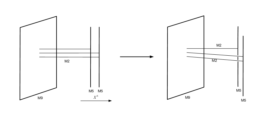
One can show that the right hand side of (28), computed up to q2superscript𝑞2q^{2} and w~1,25superscriptsubscript~𝑤125\tilde{w}_{1,2}^{5} orders from the instanton calculus, completely agrees with I(n1,n2)subscript𝐼subscript𝑛1subscript𝑛2I_{(n_{1},n_{2})} computed in the previous subsection for (n1,n2)=(1,1)subscript𝑛1subscript𝑛211(n_{1},n_{2})=(1,1), (1,2)12(1,2), (2,1)21(2,1). In particular, our proposal (4.1) is justified from the factorization (25) of the Sp(2)𝑆𝑝2Sp(2) instanton partition function at m=ϵ+𝑚subscriptitalic-ϵm=\epsilon_{+}. We show this result pictorially in Figre 8.
Refer to caption
Figure 8: String charge sector (3,2)32(3,2) for the configuration of two M5 branes probing an M9 wall. In the massless case the strings can recombine and one arrives at a configuration of a single E-string from the first M5 brane and two E-strings from the second.

5 D5 branes probing ADE singularities

In this section we study a third class of theories that arises from F-theory compactified on an elliptic Calabi-Yau threefold X𝑋X defined as follows: we take the base to be the blown-up ALE singularity of ADE type, and over each blown up 1superscript1\mathbb{P}^{1} we let the elliptic fiber have Kodaira degeneration INsubscript𝐼𝑁I_{N}. Equivalently, we can interpret this setup as Type IIB string theory with N D5 branes probing an ALF singularity of ADE type. We soon will be interested in decompactifying the circle at infinity of ALF and recover the ALE singularity. As follows from the Douglas-Moore construction Douglas:1996sw , the resulting 𝒩=(1,0)𝒩10\mathcal{N}=(1,0) six dimensional theory is captured by an affine quiver of ADE type, with the following field content: to a node i𝑖i of the affine quiver with Coxeter label disubscript𝑑𝑖d_{i} is associated a gauge group SU(diN)𝑆𝑈subscript𝑑𝑖𝑁SU(d_{i}N), and to each edge is associated bifundamental matter. Furthermore, to each node of the quiver corresponds an abelian tensor multiplet. Naively one would expect to have gauge groups U(diN)𝑈subscript𝑑𝑖𝑁U(d_{i}\,N), but one finds that in fact the abelian factor iU(1)subscriptproduct𝑖𝑈1\prod_{i}U(1) is Higgsed via a Green-Schwarz mechanism (apart from a decoupled global U(1) factor) Blum:1997mm . We now take the ALF \to ALE limit, so that the the D5 brane associated to the affine node becomes noncompact and gives rise to a global (as opposed to gauge) SU(N)𝑆𝑈𝑁SU(N) symmetry. In fact, in the Arsubscript𝐴𝑟A_{r} case, one can actually associate distinct SU(N)𝑆𝑈𝑁SU(N) global symmetries to the two non-compact half–1superscript1\mathbb{P}^{1}’s that arise from the affine node.

Of even more interest to us is the quiver gauge theory associated to the self-dual strings of the theory, which arise in F-theory as D3 branes wrapping the blown-up 1superscript1\mathbb{P}^{1}s, or equivalently in Type IIB string theory as D1 branes probing the singularity. The resulting two-dimensional quiver theory was derived for the ANsubscript𝐴𝑁A_{N} singularity by following a suitable generalization of Douglas-Moore construction Okuyama:2005gq , and is pictured in Figure 9 (this quiver is equivalent to the one depicted in Figure 1). Note that there is no restriction on the ranks of the gauge groups; the rank at any node is equal to the number of D3 branes (self-dual strings) coupled to the corresponding tensor multiplet.

Refer to caption
Figure 9: Quiver gauge theory for the non-critical strings of N𝑁N D5 branes probing an Arsubscript𝐴𝑟A_{r} singularity. Note that the global symmetry are obtained from the affine A^rsubscript^𝐴𝑟\widehat{A}_{r} quiver by ‘opening up’ the quiver at the affine node.

To avoid clutter, in this section, we work with the exponentiated variables,

t=e2πiϵ1,d=e2πiϵ2,c=e2πim.formulae-sequence𝑡superscript𝑒2𝜋𝑖subscriptitalic-ϵ1formulae-sequence𝑑superscript𝑒2𝜋𝑖subscriptitalic-ϵ2𝑐superscript𝑒2𝜋𝑖𝑚t=e^{2\pi i\epsilon_{1}},\,\,d=e^{2\pi i\epsilon_{2}},\,\,c=e^{2\pi im}. (29)

We also use exponentiated fugacity variables for gauge and global symmetries, so that, for example, θ1(z)=iq1/8(z1/2z1/2)i=1(1qi)(1qiz)(1qiz1).subscript𝜃1𝑧𝑖superscript𝑞18superscript𝑧12superscript𝑧12superscriptsubscriptproduct𝑖11superscript𝑞𝑖1superscript𝑞𝑖𝑧1superscript𝑞𝑖superscript𝑧1\theta_{1}(z)=iq^{1/8}(z^{-1/2}-z^{1/2})\prod_{i=1}^{\infty}(1-q^{i})(1-q^{i}z)(1-q^{i}z^{-1}).

With that, let us first consider an Arsubscript𝐴𝑟A_{r} singularity probed by a single D5 brane, that is we set N=1𝑁1N=1. The elliptic genus for this case, in the (n1,,nr)subscript𝑛1subscript𝑛𝑟(n_{1},\dots,n_{r}) sector corresponding to n1subscript𝑛1n_{1} strings associated to the first node, n2subscript𝑛2n_{2} for the second node, and so on, is computed by a contour integral which we write schematically as

Zn1,,nrAr,1subscriptsuperscript𝑍subscript𝐴𝑟1subscript𝑛1subscript𝑛𝑟\displaystyle Z^{A_{r},1}_{n_{1},\dots,n_{r}} =\displaystyle= (i=1r1ni!a=1niη2dza(i)2πiza(i))(i=1ra,b=1abniθ1(za(i)/zb(i))η)(i=1ra,b=1niηθ1(tdzb(i)za(i))θ1(tza(i)zb(i))θ1(dza(i)zb(i)))contour-integralsuperscriptsubscriptproduct𝑖1𝑟1subscript𝑛𝑖superscriptsubscriptproduct𝑎1subscript𝑛𝑖superscript𝜂2𝑑superscriptsubscript𝑧𝑎𝑖2𝜋𝑖superscriptsubscript𝑧𝑎𝑖superscriptsubscriptproduct𝑖1𝑟superscriptsubscriptproduct𝑎𝑏1𝑎𝑏subscript𝑛𝑖subscript𝜃1superscriptsubscript𝑧𝑎𝑖superscriptsubscript𝑧𝑏𝑖𝜂superscriptsubscriptproduct𝑖1𝑟superscriptsubscriptproduct𝑎𝑏1subscript𝑛𝑖𝜂subscript𝜃1𝑡𝑑superscriptsubscript𝑧𝑏𝑖superscriptsubscript𝑧𝑎𝑖subscript𝜃1𝑡superscriptsubscript𝑧𝑎𝑖superscriptsubscript𝑧𝑏𝑖subscript𝜃1𝑑superscriptsubscript𝑧𝑎𝑖superscriptsubscript𝑧𝑏𝑖\displaystyle\oint\left(\prod_{i=1}^{r}\frac{1}{n_{i}!}\prod_{a=1}^{n_{i}}\frac{\eta^{2}dz_{a}^{(i)}}{2\pi iz_{a}^{(i)}}\right)\left(\prod_{i=1}^{r}\prod_{\begin{subarray}{c}a,b=1\\ a\neq b\end{subarray}}^{n_{i}}\frac{\theta_{1}(z_{a}^{(i)}/z_{b}^{(i)})}{\eta}\right)\left(\prod_{i=1}^{r}\prod_{a,b=1}^{n_{i}}\frac{\eta\,\,\theta_{1}(td\frac{z_{b}^{(i)}}{z_{a}^{(i)}})}{\theta_{1}(t\frac{z_{a}^{(i)}}{z_{b}^{(i)}})\theta_{1}(d\frac{z_{a}^{(i)}}{z_{b}^{(i)}})}\right) (30)
×\displaystyle\times (i=1r1a=1nib=1ni+1θ1(cdtzb(i+1)za(i))θ1(ctdzb(i+1)za(i)))(i=2ra=1nib=1ni1θ1(ctdza(i)zb(i1))θ1(ctdza(i)zb(i1)))superscriptsubscriptproduct𝑖1𝑟1superscriptsubscriptproduct𝑎1subscript𝑛𝑖superscriptsubscriptproduct𝑏1subscript𝑛𝑖1subscript𝜃1𝑐𝑑𝑡superscriptsubscript𝑧𝑏𝑖1superscriptsubscript𝑧𝑎𝑖subscript𝜃1𝑐𝑡𝑑superscriptsubscript𝑧𝑏𝑖1superscriptsubscript𝑧𝑎𝑖superscriptsubscriptproduct𝑖2𝑟superscriptsubscriptproduct𝑎1subscript𝑛𝑖superscriptsubscriptproduct𝑏1subscript𝑛𝑖1subscript𝜃1𝑐𝑡𝑑superscriptsubscript𝑧𝑎𝑖superscriptsubscript𝑧𝑏𝑖1subscript𝜃1𝑐𝑡𝑑superscriptsubscript𝑧𝑎𝑖superscriptsubscript𝑧𝑏𝑖1\displaystyle\left(\prod_{i=1}^{r-1}\prod_{a=1}^{n_{i}}\prod_{b=1}^{n_{i+1}}\frac{\theta_{1}(c\sqrt{\frac{d}{t}}\frac{z_{b}^{(i+1)}}{z_{a}^{(i)}})}{\theta_{1}({c\sqrt{td}\frac{z_{b}^{(i+1)}}{z_{a}^{(i)}}})}\right)\left(\prod_{i=2}^{r}\prod_{a=1}^{n_{i}}\prod_{b=1}^{n_{i-1}}\frac{\theta_{1}(c\sqrt{\frac{t}{d}}\frac{z_{a}^{(i)}}{z_{b}^{(i-1)}})}{\theta_{1}(\frac{c}{\sqrt{td}}\frac{z_{a}^{(i)}}{z_{b}^{(i-1)}})}\right)
×\displaystyle\times (i=1ra=1niθ1(cza(i))θ1(c1za(i))θ1(tdza(i))θ1(td1za(i))).superscriptsubscriptproduct𝑖1𝑟superscriptsubscriptproduct𝑎1subscript𝑛𝑖subscript𝜃1𝑐superscriptsubscript𝑧𝑎𝑖subscript𝜃1𝑐1superscriptsubscript𝑧𝑎𝑖subscript𝜃1𝑡𝑑superscriptsubscript𝑧𝑎𝑖subscript𝜃1𝑡𝑑1superscriptsubscript𝑧𝑎𝑖\displaystyle\left(\prod_{i=1}^{r}\prod_{a=1}^{n_{i}}\frac{\theta_{1}(cz_{a}^{(i)})\theta_{1}(c\frac{1}{z_{a}^{(i)}})}{\theta_{1}(\sqrt{td}z_{a}^{(i)})\theta_{1}(\sqrt{td}\frac{1}{z_{a}^{(i)}})}\right).

The poles of the integral are labeled by collections of r𝑟r Young diagrams 𝒴={Y(i)}i=1r𝒴superscriptsubscriptsuperscript𝑌𝑖𝑖1𝑟\mathcal{Y}=\{Y^{(i)}\}_{i=1}^{r}, such that |Y(i)|=nisuperscript𝑌𝑖subscript𝑛𝑖|Y^{(i)}|=n_{i}, and are located at

za(i)=tx+12dy+12superscriptsubscript𝑧𝑎𝑖superscript𝑡𝑥12superscript𝑑𝑦12z_{a}^{(i)}=t^{x+\frac{1}{2}}d^{y+\frac{1}{2}} (31)

where (x,y)𝑥𝑦(x,y) are the coordinates of a𝑎a-th box in Y(i)superscript𝑌𝑖Y^{(i)} (for example, the two boxes in the diagram \square\!\square have coordinates (0,0) and (1,0)). Evaluating the residues, we get:

Zn1,,nrAr,1=𝒴(i=1r(x1,y1)Y(i)(x2,y2)Y(i)ηθ1(tx1x2+1dy1y2+1)θ1(tx1x2+1dy1y2)θ1(tx1x2dy1y2+1))subscriptsuperscript𝑍subscript𝐴𝑟1subscript𝑛1subscript𝑛𝑟subscript𝒴superscriptsubscriptproduct𝑖1𝑟subscriptproductsubscript𝑥1subscript𝑦1superscript𝑌𝑖subscript𝑥2subscript𝑦2superscript𝑌𝑖𝜂subscript𝜃1superscript𝑡subscript𝑥1subscript𝑥21superscript𝑑subscript𝑦1subscript𝑦21subscript𝜃1superscript𝑡subscript𝑥1subscript𝑥21superscript𝑑subscript𝑦1subscript𝑦2subscript𝜃1superscript𝑡subscript𝑥1subscript𝑥2superscript𝑑subscript𝑦1subscript𝑦21\displaystyle Z^{A_{r},1}_{n_{1},\dots,n_{r}}=\sum_{\mathcal{Y}}\left(\prod_{i=1}^{r}\prod_{\begin{subarray}{c}(x_{1},y_{1})\in Y^{(i)}\\ (x_{2},y_{2})\in Y^{(i)}\end{subarray}}\frac{\eta\theta_{1}(t^{x_{1}-x_{2}+1}d^{y_{1}-y_{2}+1})}{\theta_{1}(t^{x_{1}-x_{2}+1}d^{y_{1}-y_{2}})\theta_{1}(t^{x_{1}-x_{2}}d^{y_{1}-y_{2}+1})}\right)
×(i=1r(x1,y1)Y(i)(x2,y2)Y(i)(x1,y1)(x2,y2)θ1(tx1x2dy1y2)η)absentsuperscriptsubscriptproduct𝑖1𝑟subscriptproductsubscript𝑥1subscript𝑦1superscript𝑌𝑖subscript𝑥2subscript𝑦2superscript𝑌𝑖subscript𝑥1subscript𝑦1subscript𝑥2subscript𝑦2subscript𝜃1superscript𝑡subscript𝑥1subscript𝑥2superscript𝑑subscript𝑦1subscript𝑦2𝜂\displaystyle\times\left(\prod_{i=1}^{r}\prod_{\begin{subarray}{c}(x_{1},y_{1})\in Y^{(i)}\\ (x_{2},y_{2})\in Y^{(i)}\\ (x_{1},y_{1})\neq(x_{2},y_{2})\end{subarray}}\frac{\theta_{1}(t^{x_{1}-x_{2}}d^{y_{1}-y_{2}})}{\eta}\right)
×(i=1r1(x1,y1)Y(i+1)(x2,y2)Y(i)θ1(ctx1x212dy1y2+12)θ1(ctx1x2+12dy1y2+12))(i=2r(x1,y1)Y(i)(x2,y2)Y(i1)θ1(ctx1x2+12dy1y212)θ1(ctx1x212dy1y212))absentsuperscriptsubscriptproduct𝑖1𝑟1subscriptproductsubscript𝑥1subscript𝑦1superscript𝑌𝑖1subscript𝑥2subscript𝑦2superscript𝑌𝑖subscript𝜃1𝑐superscript𝑡subscript𝑥1subscript𝑥212superscript𝑑subscript𝑦1subscript𝑦212subscript𝜃1𝑐superscript𝑡subscript𝑥1subscript𝑥212superscript𝑑subscript𝑦1subscript𝑦212superscriptsubscriptproduct𝑖2𝑟subscriptproductsubscript𝑥1subscript𝑦1superscript𝑌𝑖subscript𝑥2subscript𝑦2superscript𝑌𝑖1subscript𝜃1𝑐superscript𝑡subscript𝑥1subscript𝑥212superscript𝑑subscript𝑦1subscript𝑦212subscript𝜃1𝑐superscript𝑡subscript𝑥1subscript𝑥212superscript𝑑subscript𝑦1subscript𝑦212\displaystyle\times\left(\prod_{i=1}^{r-1}\prod_{\begin{subarray}{c}(x_{1},y_{1})\in Y^{(i+1)}\\ (x_{2},y_{2})\in Y^{(i)}\end{subarray}}\frac{\theta_{1}(ct^{x_{1}-x_{2}-\frac{1}{2}}d^{y_{1}-y_{2}+\frac{1}{2}})}{\theta_{1}(ct^{x_{1}-x_{2}+\frac{1}{2}}d^{y_{1}-y_{2}+\frac{1}{2}})}\right)\left(\prod_{i=2}^{r}\prod_{\begin{subarray}{c}(x_{1},y_{1})\in Y^{(i)}\\ (x_{2},y_{2})\in Y^{(i-1)}\end{subarray}}\frac{\theta_{1}(ct^{x_{1}-x_{2}+\frac{1}{2}}d^{y_{1}-y_{2}-\frac{1}{2}})}{\theta_{1}(ct^{x_{1}-x_{2}-\frac{1}{2}}d^{y_{1}-y_{2}-\frac{1}{2}})}\right)
×(i=1r(x1,y1)Y(i)θ1(ctx1+12dy1+12)θ1(ctx112dy112)θ1(tx1+1dy1+1)η)(i=1r(x1,y1)Y(i)(x1,y1)(0,0)ηθ1(tx1dy1)).absentsuperscriptsubscriptproduct𝑖1𝑟subscriptproductsubscript𝑥1subscript𝑦1superscript𝑌𝑖subscript𝜃1𝑐superscript𝑡subscript𝑥112superscript𝑑subscript𝑦112subscript𝜃1𝑐superscript𝑡subscript𝑥112superscript𝑑subscript𝑦112subscript𝜃1superscript𝑡subscript𝑥11superscript𝑑subscript𝑦11𝜂superscriptsubscriptproduct𝑖1𝑟subscriptproductsubscript𝑥1subscript𝑦1superscript𝑌𝑖subscript𝑥1subscript𝑦100𝜂subscript𝜃1superscript𝑡subscript𝑥1superscript𝑑subscript𝑦1\displaystyle\times\left(\prod_{i=1}^{r}\prod_{(x_{1},y_{1})\in Y^{(i)}}\frac{\theta_{1}(ct^{x_{1}+\frac{1}{2}}d^{y_{1}+\frac{1}{2}})\theta_{1}(ct^{-x_{1}-\frac{1}{2}}d^{-y_{1}-\frac{1}{2}})}{\theta_{1}(t^{x_{1}+1}d^{y_{1}+1})\eta}\right)\left(\prod_{i=1}^{r}\prod_{\begin{subarray}{c}(x_{1},y_{1})\in Y^{(i)}\\ (x_{1},y_{1})\neq(0,0)\end{subarray}}\frac{\eta}{\theta_{1}(t^{-x_{1}}d^{-y_{1}})}\right).

The computation for an arbitrary number N𝑁N of D5 branes is only slightly more involved; the flavor symmetry group now also includes a SU(N)r+2𝑆𝑈superscript𝑁𝑟2SU(N)^{r+2} factor; for the factor of SU(N)𝑆𝑈𝑁SU(N) corresponding to the i𝑖i-th node, we introduce fugacities sb(i),b=1,,Nformulae-sequencesuperscriptsubscript𝑠𝑏𝑖𝑏1𝑁s_{b}^{(i)},\>b=1,\ldots,N. These fugacities obey sb(i)=1productsuperscriptsubscript𝑠𝑏𝑖1\prod s_{b}^{(i)}=1. We label the leftmost and rightmost flavor symmetry nodes in Figure 9 respectively by i=0𝑖0i=0 and i=r+1𝑖𝑟1i=r+1.222In the ALE limit, we are free to assign independent fugacities to these two flavor symmetry groups The elliptic genus is now given by:

Zn1,,nrAr,Nsubscriptsuperscript𝑍subscript𝐴𝑟𝑁subscript𝑛1subscript𝑛𝑟\displaystyle Z^{A_{r},N}_{n_{1},\dots,n_{r}} =\displaystyle= (i=1r1ni!a=1niη2dza(i)2πiza(i))(i=1ra,b=1abniθ1(za(i)/zb(i))η)(i=1ra,b=1niηθ1(tdzb(i)za(i))θ1(tza(i)zb(i))θ1(dza(i)zb(i)))contour-integralsuperscriptsubscriptproduct𝑖1𝑟1subscript𝑛𝑖superscriptsubscriptproduct𝑎1subscript𝑛𝑖superscript𝜂2𝑑superscriptsubscript𝑧𝑎𝑖2𝜋𝑖superscriptsubscript𝑧𝑎𝑖superscriptsubscriptproduct𝑖1𝑟superscriptsubscriptproduct𝑎𝑏1𝑎𝑏subscript𝑛𝑖subscript𝜃1superscriptsubscript𝑧𝑎𝑖superscriptsubscript𝑧𝑏𝑖𝜂superscriptsubscriptproduct𝑖1𝑟superscriptsubscriptproduct𝑎𝑏1subscript𝑛𝑖𝜂subscript𝜃1𝑡𝑑superscriptsubscript𝑧𝑏𝑖superscriptsubscript𝑧𝑎𝑖subscript𝜃1𝑡superscriptsubscript𝑧𝑎𝑖superscriptsubscript𝑧𝑏𝑖subscript𝜃1𝑑superscriptsubscript𝑧𝑎𝑖superscriptsubscript𝑧𝑏𝑖\displaystyle\oint\left(\prod_{i=1}^{r}\frac{1}{n_{i}!}\prod_{a=1}^{n_{i}}\frac{\eta^{2}dz_{a}^{(i)}}{2\pi iz_{a}^{(i)}}\right)\left(\prod_{i=1}^{r}\prod_{\begin{subarray}{c}a,b=1\\ a\neq b\end{subarray}}^{n_{i}}\frac{\theta_{1}(z_{a}^{(i)}/z_{b}^{(i)})}{\eta}\right)\left(\prod_{i=1}^{r}\prod_{a,b=1}^{n_{i}}\frac{\eta\,\,\theta_{1}(td\frac{z_{b}^{(i)}}{z_{a}^{(i)}})}{\theta_{1}(t\frac{z_{a}^{(i)}}{z_{b}^{(i)}})\theta_{1}(d\frac{z_{a}^{(i)}}{z_{b}^{(i)}})}\right) (33)
×\displaystyle\times (i=1r1a=1nib=1ni+1θ1(cdtzb(i+1)za(i))θ1(ctdzb(i+1)za(i)))(i=2ra=1nib=1ni1θ1(ctdza(i)zb(i1))θ1(ctdza(i)zb(i1)))superscriptsubscriptproduct𝑖1𝑟1superscriptsubscriptproduct𝑎1subscript𝑛𝑖superscriptsubscriptproduct𝑏1subscript𝑛𝑖1subscript𝜃1𝑐𝑑𝑡superscriptsubscript𝑧𝑏𝑖1superscriptsubscript𝑧𝑎𝑖subscript𝜃1𝑐𝑡𝑑superscriptsubscript𝑧𝑏𝑖1superscriptsubscript𝑧𝑎𝑖superscriptsubscriptproduct𝑖2𝑟superscriptsubscriptproduct𝑎1subscript𝑛𝑖superscriptsubscriptproduct𝑏1subscript𝑛𝑖1subscript𝜃1𝑐𝑡𝑑superscriptsubscript𝑧𝑎𝑖superscriptsubscript𝑧𝑏𝑖1subscript𝜃1𝑐𝑡𝑑superscriptsubscript𝑧𝑎𝑖superscriptsubscript𝑧𝑏𝑖1\displaystyle\left(\prod_{i=1}^{r-1}\prod_{a=1}^{n_{i}}\prod_{b=1}^{n_{i+1}}\frac{\theta_{1}(c\sqrt{\frac{d}{t}}\frac{z_{b}^{(i+1)}}{z_{a}^{(i)}})}{\theta_{1}({c\sqrt{td}\frac{z_{b}^{(i+1)}}{z_{a}^{(i)}}})}\right)\left(\prod_{i=2}^{r}\prod_{a=1}^{n_{i}}\prod_{b=1}^{n_{i-1}}\frac{\theta_{1}(c\sqrt{\frac{t}{d}}\frac{z_{a}^{(i)}}{z_{b}^{(i-1)}})}{\theta_{1}(\frac{c}{\sqrt{td}}\frac{z_{a}^{(i)}}{z_{b}^{(i-1)}})}\right)
×\displaystyle\times (i=1ra=1nib=1Nθ1(cza(i)sb(i1))θ1(csb(i+1)za(i))θ1(tdza(i)sb(i))θ1(tdsb(i)za(i))).superscriptsubscriptproduct𝑖1𝑟superscriptsubscriptproduct𝑎1subscript𝑛𝑖superscriptsubscriptproduct𝑏1𝑁subscript𝜃1𝑐superscriptsubscript𝑧𝑎𝑖superscriptsubscript𝑠𝑏𝑖1subscript𝜃1𝑐superscriptsubscript𝑠𝑏𝑖1superscriptsubscript𝑧𝑎𝑖subscript𝜃1𝑡𝑑superscriptsubscript𝑧𝑎𝑖superscriptsubscript𝑠𝑏𝑖subscript𝜃1𝑡𝑑superscriptsubscript𝑠𝑏𝑖superscriptsubscript𝑧𝑎𝑖\displaystyle\left(\prod_{i=1}^{r}\prod_{a=1}^{n_{i}}\prod_{b=1}^{N}\frac{\theta_{1}(c\frac{z_{a}^{(i)}}{s_{b}^{(i-1)}})\theta_{1}(c\frac{s_{b}^{(i+1)}}{z_{a}^{(i)}})}{\theta_{1}(\sqrt{td}\frac{z_{a}^{(i)}}{s_{b}^{(i)}})\theta_{1}(\sqrt{td}\frac{s_{b}^{(i)}}{z_{a}^{(i)}})}\right).

The poles of this integral are classified by collections 𝒴𝒴\mathcal{Y} of colored Young diagrams: 𝒴={{Yi(i)}i=1N}i=1r𝒴superscriptsubscriptsuperscriptsubscriptsubscriptsuperscript𝑌𝑖subscript𝑖subscript𝑖1𝑁𝑖1𝑟\mathcal{Y}=\{\{Y^{(i)}_{\ell_{i}}\}_{\ell_{i}=1}^{N}\}_{i=1}^{r}, subject to the constraint i=1N|Yi(i)|=nisuperscriptsubscriptsubscript𝑖1𝑁superscriptsubscript𝑌subscript𝑖𝑖subscript𝑛𝑖\sum_{\ell_{i}=1}^{N}|Y_{\ell_{i}}^{(i)}|=n_{i}. The pole associated to the a𝑎a-box in the Young diagram Yi(i)superscriptsubscript𝑌subscript𝑖𝑖Y_{\ell_{i}}^{(i)}, with coordinates (x,y)𝑥𝑦(x,y), is at

za(i)=si(i)t12+xd12+y.superscriptsubscript𝑧𝑎𝑖superscriptsubscript𝑠subscript𝑖𝑖superscript𝑡12𝑥superscript𝑑12𝑦z_{a}^{(i)}=s_{\ell_{i}}^{(i)}t^{\frac{1}{2}+x}d^{\frac{1}{2}+y}. (34)

Evaluating the residues we find:

Zn1,,nrAr,N=𝒴(i=1r,m=1N(x1,y1)Y(i)(x2,y2)Ym(i)θ1(tx1x2dy1y2)θ1(s(i)sm(i)tx1x2+1dy1y2+1)θ1(s(i)sm(i)tx1x2+1dy1y2)θ1(s(i)sm(i)tx1x2dy1y2+1))subscriptsuperscript𝑍subscript𝐴𝑟𝑁subscript𝑛1subscript𝑛𝑟subscript𝒴superscriptsubscriptproduct𝑖1𝑟superscriptsubscriptproduct𝑚1𝑁subscriptproductsubscript𝑥1subscript𝑦1subscriptsuperscript𝑌𝑖subscript𝑥2subscript𝑦2subscriptsuperscript𝑌𝑖𝑚subscript𝜃1superscript𝑡subscript𝑥1subscript𝑥2superscript𝑑subscript𝑦1subscript𝑦2subscript𝜃1superscriptsubscript𝑠𝑖superscriptsubscript𝑠𝑚𝑖superscript𝑡subscript𝑥1subscript𝑥21superscript𝑑subscript𝑦1subscript𝑦21subscript𝜃1superscriptsubscript𝑠𝑖superscriptsubscript𝑠𝑚𝑖superscript𝑡subscript𝑥1subscript𝑥21superscript𝑑subscript𝑦1subscript𝑦2subscript𝜃1superscriptsubscript𝑠𝑖superscriptsubscript𝑠𝑚𝑖superscript𝑡subscript𝑥1subscript𝑥2superscript𝑑subscript𝑦1subscript𝑦21\displaystyle Z^{A_{r},N}_{n_{1},\dots,n_{r}}=\sum_{\mathcal{Y}}\left(\prod_{i=1}^{r}\prod_{\ell,m=1}^{N}\prod_{\begin{subarray}{c}(x_{1},y_{1})\in Y^{(i)}_{\ell}\\ (x_{2},y_{2})\in Y^{(i)}_{m}\end{subarray}}\frac{\theta_{1}(t^{{x_{1}}-{x_{2}}}d^{{y_{1}}-{y_{2}}})\theta_{1}(\frac{s_{\ell}^{(i)}}{s_{m}^{(i)}}t^{{x_{1}}-{x_{2}}+1}d^{{y_{1}}-{y_{2}}+1})}{\theta_{1}(\frac{s_{\ell}^{(i)}}{s_{m}^{(i)}}t^{{x_{1}}-{x_{2}}+1}d^{{y_{1}}-{y_{2}}})\theta_{1}(\frac{s_{\ell}^{(i)}}{s_{m}^{(i)}}t^{{x_{1}}-{x_{2}}}d^{{y_{1}}-{y_{2}}+1})}\right)
×(i=1r1,m=1N(x1,y1)Y(i)(x2,y2)Ym(i+1)θ1(c1s(i)sm(i+1)tx1x2+12dy1y212)θ1(c1s(i)sm(i+1)tx1x212dy1y212))absentsuperscriptsubscriptproduct𝑖1𝑟1superscriptsubscriptproduct𝑚1𝑁subscriptproductsubscript𝑥1subscript𝑦1subscriptsuperscript𝑌𝑖subscript𝑥2subscript𝑦2subscriptsuperscript𝑌𝑖1𝑚subscript𝜃1superscript𝑐1superscriptsubscript𝑠𝑖superscriptsubscript𝑠𝑚𝑖1superscript𝑡subscript𝑥1subscript𝑥212superscript𝑑subscript𝑦1subscript𝑦212subscript𝜃1superscript𝑐1superscriptsubscript𝑠𝑖superscriptsubscript𝑠𝑚𝑖1superscript𝑡subscript𝑥1subscript𝑥212superscript𝑑subscript𝑦1subscript𝑦212\displaystyle\times\left(\prod_{i=1}^{r-1}\prod_{\ell,m=1}^{N}\prod_{\begin{subarray}{c}(x_{1},y_{1})\in Y^{(i)}_{\ell}\\ (x_{2},y_{2})\in Y^{(i+1)}_{m}\end{subarray}}\frac{\theta_{1}(c^{-1}\frac{s_{\ell}^{(i)}}{s_{m}^{(i+1)}}t^{{x_{1}}-{x_{2}}+\frac{1}{2}}d^{{y_{1}}-{y_{2}}-\frac{1}{2}})}{\theta_{1}(c^{-1}\frac{s_{\ell}^{(i)}}{s_{m}^{(i+1)}}t^{{x_{1}}-{x_{2}}-\frac{1}{2}}d^{{y_{1}}-{y_{2}}-\frac{1}{2}})}\right)
×(i=2r,m=1N(x1,y1)Y(i)(x2,y2)Ym(i1)θ1(cs(i)sm(i1)tx1x2+12dy1y212)θ1(cs(i)sm(i1)tx1x212dy1y212))×\displaystyle\times\left(\prod_{i=2}^{r}\prod_{\ell,m=1}^{N}\prod_{\begin{subarray}{c}(x_{1},y_{1})\in Y^{(i)}_{\ell}\\ (x_{2},y_{2})\in Y^{(i-1)}_{m}\end{subarray}}\frac{\theta_{1}(c\frac{s_{\ell}^{(i)}}{s_{m}^{(i-1)}}t^{{x_{1}}-{x_{2}}+\frac{1}{2}}d^{{y_{1}}-{y_{2}}-\frac{1}{2}})}{\theta_{1}(c\frac{s_{\ell}^{(i)}}{s_{m}^{(i-1)}}t^{{x_{1}}-{x_{2}}-\frac{1}{2}}d^{{y_{1}}-{y_{2}}-\frac{1}{2}})}\right)\times
×(i=1r,m=1N(x,y)Y(i)θ1(cs(i)sm(i1)tx+12dy+12)θ1(csm(i+1)s(i)tx12dy12)θ1(s(i)sm(i)tx+1dy+1)θ1(sm(i)s(i)txdy)).absentsuperscriptsubscriptproduct𝑖1𝑟superscriptsubscriptproduct𝑚1𝑁subscriptproduct𝑥𝑦subscriptsuperscript𝑌𝑖subscript𝜃1𝑐superscriptsubscript𝑠𝑖superscriptsubscript𝑠𝑚𝑖1superscript𝑡𝑥12superscript𝑑𝑦12subscript𝜃1𝑐superscriptsubscript𝑠𝑚𝑖1superscriptsubscript𝑠𝑖superscript𝑡𝑥12superscript𝑑𝑦12subscript𝜃1superscriptsubscript𝑠𝑖superscriptsubscript𝑠𝑚𝑖superscript𝑡𝑥1superscript𝑑𝑦1subscript𝜃1superscriptsubscript𝑠𝑚𝑖superscriptsubscript𝑠𝑖superscript𝑡𝑥superscript𝑑𝑦\displaystyle\times\left(\prod_{i=1}^{r}\prod_{\ell,m=1}^{N}\prod_{(x,y)\in Y^{(i)}_{\ell}}\frac{\theta_{1}(c\frac{s_{\ell}^{(i)}}{s_{m}^{(i-1)}}t^{x+\frac{1}{2}}d^{y+\frac{1}{2}})\theta_{1}(c\frac{s_{m}^{(i+1)}}{s_{\ell}^{(i)}}t^{-x-\frac{1}{2}}d^{-y-\frac{1}{2}})}{\theta_{1}(\frac{s_{\ell}^{(i)}}{s_{m}^{(i)}}t^{x+1}d^{y+1})\theta_{1}(\frac{s_{m}^{(i)}}{s_{\ell}^{(i)}}t^{-x}d^{-y})}\right). (35)

Note that the products include various factors of θ1(1)subscript𝜃11\theta_{1}(1), which however completely cancel against each other.
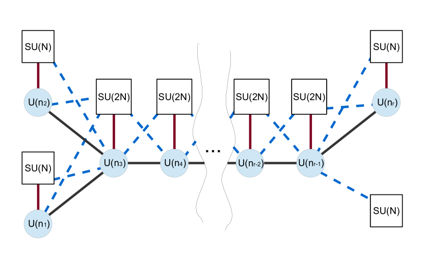
Refer to caption
Figure 10: Quiver gauge theory for the non-critical strings of N𝑁N D5 branes probing a Drsubscript𝐷𝑟D_{r} singularity.
Refer to caption
Figure 11: Oriented E^6subscript^𝐸6\widehat{E}_{6} quiver with a particular labelling of the nodes i𝑖i. The numbers in the parentheses represent the Coxeter labels disubscript𝑑𝑖d_{i}.
Refer to caption
Figure 12: Quiver gauge theory for the non-critical strings of N𝑁N D5 branes probing an E6subscript𝐸6E_{6} singularity.
Refer to caption
Figure 13: Quiver gauge theory for the non-critical strings of N𝑁N D5 branes probing an E7subscript𝐸7E_{7} singularity.
Refer to caption
Figure 14: Quiver gauge theory for the non-critical strings of N𝑁N D5 branes probing an E8subscript𝐸8E_{8} singularity.

Finally we pass to the case of N𝑁N D5 branes probing singularities of type Drsubscript𝐷𝑟D_{r} or E6,E7,E8subscript𝐸6subscript𝐸7subscript𝐸8E_{6},E_{7},E_{8}. Their two-dimensional quivers are pictured in Figures 10 –14. An important difference between the A𝐴A case and the D𝐷D and E𝐸E cases is that in the latter the U(1)m𝑈subscript1𝑚U(1)_{m} symmetry is anomalous. Hence, we will not be able to refine the index with the corresponding fugacity c𝑐c. The Lagrangian of the (0,4)04(0,4) theory is chiral. This is apparent from the fact that ΛQsuperscriptΛ𝑄\Lambda^{Q} and ΛQ~superscriptΛ~𝑄\Lambda^{\tilde{Q}} transform oppositely. The same is the case with the fields ΛB,ΛB~,ΣsuperscriptΛ𝐵superscriptΛ~𝐵Σ\Lambda^{B},\Lambda^{\tilde{B}},\Sigma and ΦΦ\Phi. Although, for D𝐷D and E𝐸E type quivers there is no preferred orientation of, say, the ΦΦ\Phi arrow. But as it will soon become clear, the elliptic genus of the theory does not depend on the choice of this orientation.

Let us label the gauge nodes by an index i𝑖i taking the values from 111 to r𝑟r. The range of the index for the flavor nodes, on the other hand, runs from 00 to r𝑟r, where i=0𝑖0i=0 corresponds to the affine node. Let sb(i),b=1,,diNformulae-sequencesuperscriptsubscript𝑠𝑏𝑖𝑏1subscript𝑑𝑖𝑁s_{b}^{(i)},\>b=1,\ldots,d_{i}N be the fugacity corresponding to the flavor symmetry group SU(diN)𝑆𝑈subscript𝑑𝑖𝑁SU(d_{i}N) where disubscript𝑑𝑖d_{i} is the Coxeter label of the node i𝑖i. These fugacities obey sb(i)=1productsuperscriptsubscript𝑠𝑏𝑖1\prod s_{b}^{(i)}=1. Let Mijsubscript𝑀𝑖𝑗M_{ij} be the adjacency matrix of the quiver with some orientation.

For example, Figure 11 shows the Coxeter labels of the affine E6subscript𝐸6E_{6} quiver together with a particular labeling. The corresponding adjacency matrix is given by

ME^6=(0010000000100000001000000100000001000000010000000).superscript𝑀subscript^𝐸60010000000100000001000000100000001000000010000000M^{\widehat{E}_{6}}=\left(\begin{array}[]{ccccccc}0&0&1&0&0&0&0\\ 0&0&0&1&0&0&0\\ 0&0&0&0&1&0&0\\ 0&0&0&0&1&0&0\\ 0&0&0&0&0&1&0\\ 0&0&0&0&0&0&1\\ 0&0&0&0&0&0&0\end{array}\right). (36)

The elliptic genus of the 2d2𝑑2d theory for G=Dr,E6,E7,E8𝐺subscript𝐷𝑟subscript𝐸6subscript𝐸7subscript𝐸8G=D_{r},E_{6},E_{7},E_{8} is then given by

Zn1,,nrG,Nsubscriptsuperscript𝑍𝐺𝑁subscript𝑛1subscript𝑛𝑟\displaystyle Z^{G,N}_{n_{1},\dots,n_{r}} =\displaystyle= (i=1r1ni!a=1niη2dza(i)2πiza(i))(i=1ra,b=1abniθ1(za(i)/zb(i))η)(i=1ra,b=1niηθ1(tdzb(i)za(i))θ1(tza(i)zb(i))θ1(dza(i)zb(i)))contour-integralsuperscriptsubscriptproduct𝑖1𝑟1subscript𝑛𝑖superscriptsubscriptproduct𝑎1subscript𝑛𝑖superscript𝜂2𝑑superscriptsubscript𝑧𝑎𝑖2𝜋𝑖superscriptsubscript𝑧𝑎𝑖superscriptsubscriptproduct𝑖1𝑟superscriptsubscriptproduct𝑎𝑏1𝑎𝑏subscript𝑛𝑖subscript𝜃1superscriptsubscript𝑧𝑎𝑖superscriptsubscript𝑧𝑏𝑖𝜂superscriptsubscriptproduct𝑖1𝑟superscriptsubscriptproduct𝑎𝑏1subscript𝑛𝑖𝜂subscript𝜃1𝑡𝑑superscriptsubscript𝑧𝑏𝑖superscriptsubscript𝑧𝑎𝑖subscript𝜃1𝑡superscriptsubscript𝑧𝑎𝑖superscriptsubscript𝑧𝑏𝑖subscript𝜃1𝑑superscriptsubscript𝑧𝑎𝑖superscriptsubscript𝑧𝑏𝑖\displaystyle\oint\left(\prod_{i=1}^{r}\frac{1}{n_{i}!}\prod_{a=1}^{n_{i}}\frac{\eta^{2}dz_{a}^{(i)}}{2\pi iz_{a}^{(i)}}\right)\left(\prod_{i=1}^{r}\prod_{\begin{subarray}{c}a,b=1\\ a\neq b\end{subarray}}^{n_{i}}\frac{\theta_{1}(z_{a}^{(i)}/z_{b}^{(i)})}{\eta}\right)\left(\prod_{i=1}^{r}\prod_{a,b=1}^{n_{i}}\frac{\eta\,\,\theta_{1}(td\frac{z_{b}^{(i)}}{z_{a}^{(i)}})}{\theta_{1}(t\frac{z_{a}^{(i)}}{z_{b}^{(i)}})\theta_{1}(d\frac{z_{a}^{(i)}}{z_{b}^{(i)}})}\right)
×\displaystyle\times (i=1ra=1nib=1Ndiη2θ1(tdza(i)sb(i))θ1(tdsb(i)za(i)))(j=0rb=1djN(θ1(za(i)sb(j))η)Mij(θ1(sb(j)za(i))η)Mji)superscriptsubscriptproduct𝑖1𝑟superscriptsubscriptproduct𝑎1subscript𝑛𝑖superscriptsubscriptproduct𝑏1𝑁subscript𝑑𝑖superscript𝜂2subscript𝜃1𝑡𝑑superscriptsubscript𝑧𝑎𝑖superscriptsubscript𝑠𝑏𝑖subscript𝜃1𝑡𝑑superscriptsubscript𝑠𝑏𝑖superscriptsubscript𝑧𝑎𝑖superscriptsubscriptproduct𝑗0𝑟superscriptsubscriptproduct𝑏1subscript𝑑𝑗𝑁superscriptsubscript𝜃1superscriptsubscript𝑧𝑎𝑖superscriptsubscript𝑠𝑏𝑗𝜂subscript𝑀𝑖𝑗superscriptsubscript𝜃1superscriptsubscript𝑠𝑏𝑗superscriptsubscript𝑧𝑎𝑖𝜂subscript𝑀𝑗𝑖\displaystyle\left(\prod_{i=1}^{r}\prod_{a=1}^{n_{i}}\prod_{b=1}^{Nd_{i}}\frac{\eta^{2}}{\theta_{1}(\sqrt{td}\frac{z_{a}^{(i)}}{s_{b}^{(i)}})\theta_{1}(\sqrt{td}\frac{s_{b}^{(i)}}{z_{a}^{(i)}})}\right)\left(\prod_{j=0}^{r}\prod_{b=1}^{d_{j}N}\left(\frac{\theta_{1}(\frac{z_{a}^{(i)}}{s_{b}^{(j)}})}{\eta}\right)^{M_{ij}}\left(\frac{\theta_{1}(\frac{s_{b}^{(j)}}{z_{a}^{(i)}})}{\eta}\right)^{M_{ji}}\right)
×\displaystyle\times (i,j=1ra=1nib=1nj(θ1(dtza(i)zb(j))θ1(tdza(i)zb(j))θ1(1tdzb(j)za(i))θ1(1tdza(i)zb(j)))Mij).superscriptsubscriptproduct𝑖𝑗1𝑟superscriptsubscriptproduct𝑎1subscript𝑛𝑖superscriptsubscriptproduct𝑏1subscript𝑛𝑗superscriptsubscript𝜃1𝑑𝑡superscriptsubscript𝑧𝑎𝑖superscriptsubscript𝑧𝑏𝑗subscript𝜃1𝑡𝑑superscriptsubscript𝑧𝑎𝑖superscriptsubscript𝑧𝑏𝑗subscript𝜃11𝑡𝑑superscriptsubscript𝑧𝑏𝑗superscriptsubscript𝑧𝑎𝑖subscript𝜃11𝑡𝑑superscriptsubscript𝑧𝑎𝑖superscriptsubscript𝑧𝑏𝑗subscript𝑀𝑖𝑗\displaystyle\left(\prod_{i,j=1}^{r}\prod_{a=1}^{n_{i}}\prod_{b=1}^{n_{j}}\left(\frac{\theta_{1}(\sqrt{\frac{d}{t}}\frac{z_{a}^{(i)}}{z_{b}^{(j)}})\theta_{1}(\sqrt{\frac{t}{d}}\frac{z_{a}^{(i)}}{z_{b}^{(j)}})}{\theta_{1}(\frac{1}{\sqrt{td}}\frac{z_{b}^{(j)}}{z_{a}^{(i)}})\theta_{1}(\frac{1}{\sqrt{td}}\frac{z_{a}^{(i)}}{z_{b}^{(j)}})}\right)^{M_{ij}}\right).

Using the identity θ1(x)=θ1(x1)subscript𝜃1𝑥subscript𝜃1superscript𝑥1\theta_{1}(x)=-\theta_{1}(x^{-1}) we get (up to a sign):

Zn1,,nrG,Nsubscriptsuperscript𝑍𝐺𝑁subscript𝑛1subscript𝑛𝑟\displaystyle Z^{G,N}_{n_{1},\dots,n_{r}} =\displaystyle= (i=1r1ni!a=1niη2dza(i)2πiza(i))(i=1ra,b=1abniθ1(za(i)/zb(i))η)(i=1ra,b=1niηθ1(tdzb(i)za(i))θ1(tza(i)zb(i))θ1(dza(i)zb(i)))contour-integralsuperscriptsubscriptproduct𝑖1𝑟1subscript𝑛𝑖superscriptsubscriptproduct𝑎1subscript𝑛𝑖superscript𝜂2𝑑superscriptsubscript𝑧𝑎𝑖2𝜋𝑖superscriptsubscript𝑧𝑎𝑖superscriptsubscriptproduct𝑖1𝑟superscriptsubscriptproduct𝑎𝑏1𝑎𝑏subscript𝑛𝑖subscript𝜃1superscriptsubscript𝑧𝑎𝑖superscriptsubscript𝑧𝑏𝑖𝜂superscriptsubscriptproduct𝑖1𝑟superscriptsubscriptproduct𝑎𝑏1subscript𝑛𝑖𝜂subscript𝜃1𝑡𝑑superscriptsubscript𝑧𝑏𝑖superscriptsubscript𝑧𝑎𝑖subscript𝜃1𝑡superscriptsubscript𝑧𝑎𝑖superscriptsubscript𝑧𝑏𝑖subscript𝜃1𝑑superscriptsubscript𝑧𝑎𝑖superscriptsubscript𝑧𝑏𝑖\displaystyle\!\oint\left(\prod_{i=1}^{r}\frac{1}{n_{i}!}\prod_{a=1}^{n_{i}}\frac{\eta^{2}dz_{a}^{(i)}}{2\pi iz_{a}^{(i)}}\right)\!\left(\prod_{i=1}^{r}\prod_{\begin{subarray}{c}a,b=1\\ a\neq b\end{subarray}}^{n_{i}}\frac{\theta_{1}(z_{a}^{(i)}/z_{b}^{(i)})}{\eta}\right)\!\left(\prod_{i=1}^{r}\prod_{a,b=1}^{n_{i}}\frac{\eta\,\,\theta_{1}(td\frac{z_{b}^{(i)}}{z_{a}^{(i)}})}{\theta_{1}(t\frac{z_{a}^{(i)}}{z_{b}^{(i)}})\theta_{1}(d\frac{z_{a}^{(i)}}{z_{b}^{(i)}})}\right) (38)
×\displaystyle\times (i=1ra=1nib=1Ndiη2θ1(tdza(i)sb(i))θ1(tdsb(i)za(i)))(i=1rj=0rb=1djN(θ1(sb(j)za(i))η)Mij+MijT)superscriptsubscriptproduct𝑖1𝑟superscriptsubscriptproduct𝑎1subscript𝑛𝑖superscriptsubscriptproduct𝑏1𝑁subscript𝑑𝑖superscript𝜂2subscript𝜃1𝑡𝑑superscriptsubscript𝑧𝑎𝑖superscriptsubscript𝑠𝑏𝑖subscript𝜃1𝑡𝑑superscriptsubscript𝑠𝑏𝑖superscriptsubscript𝑧𝑎𝑖superscriptsubscriptproduct𝑖1𝑟superscriptsubscriptproduct𝑗0𝑟superscriptsubscriptproduct𝑏1subscript𝑑𝑗𝑁superscriptsubscript𝜃1superscriptsubscript𝑠𝑏𝑗superscriptsubscript𝑧𝑎𝑖𝜂subscript𝑀𝑖𝑗subscriptsuperscript𝑀𝑇𝑖𝑗\displaystyle\left(\prod_{i=1}^{r}\prod_{a=1}^{n_{i}}\prod_{b=1}^{Nd_{i}}\frac{\eta^{2}}{\theta_{1}(\sqrt{td}\frac{z_{a}^{(i)}}{s_{b}^{(i)}})\theta_{1}(\sqrt{td}\frac{s_{b}^{(i)}}{z_{a}^{(i)}})}\right)\left(\prod_{i=1}^{r}\prod_{j=0}^{r}\prod_{b=1}^{d_{j}N}\left(\frac{\theta_{1}(\frac{s_{b}^{(j)}}{z_{a}^{(i)}})}{\eta}\right)^{M_{ij}+M^{T}_{ij}}\right)
×\displaystyle\times (i,j=1ra=1nib=1nj(θ1(dtza(i)zb(j))θ1(1tdza(i)zb(j)))Mij+MijT).superscriptsubscriptproduct𝑖𝑗1𝑟superscriptsubscriptproduct𝑎1subscript𝑛𝑖superscriptsubscriptproduct𝑏1subscript𝑛𝑗superscriptsubscript𝜃1𝑑𝑡superscriptsubscript𝑧𝑎𝑖superscriptsubscript𝑧𝑏𝑗subscript𝜃11𝑡𝑑superscriptsubscript𝑧𝑎𝑖superscriptsubscript𝑧𝑏𝑗subscript𝑀𝑖𝑗subscriptsuperscript𝑀𝑇𝑖𝑗\displaystyle\left(\prod_{i,j=1}^{r}\prod_{a=1}^{n_{i}}\prod_{b=1}^{n_{j}}\left(\frac{\theta_{1}(\sqrt{\frac{d}{t}}\frac{z_{a}^{(i)}}{z_{b}^{(j)}})}{\theta_{1}(\frac{1}{\sqrt{td}}\frac{z_{a}^{(i)}}{z_{b}^{(j)}})}\right)^{M_{ij}+M^{T}_{ij}}\right).

As it is clear from the expression, the elliptic genus depends only on the combination Mij+MijTAijsubscript𝑀𝑖𝑗subscriptsuperscript𝑀𝑇𝑖𝑗subscript𝐴𝑖𝑗M_{ij}+M^{T}_{ij}\equiv A_{ij}, the undirected adjacency matrix of the affine D𝐷D or E𝐸E quiver. The poles of this integral are classified by collections 𝒴𝒴\mathcal{Y} of colored Young diagrams: 𝒴={{Yi(i)}i=1diN}i=1r𝒴superscriptsubscriptsuperscriptsubscriptsubscriptsuperscript𝑌𝑖subscript𝑖subscript𝑖1subscript𝑑𝑖𝑁𝑖1𝑟\mathcal{Y}=\{\{Y^{(i)}_{\ell_{i}}\}_{\ell_{i}=1}^{d_{i}N}\}_{i=1}^{r}, subject to the constraint i=1diN|Yi(i)|=nisuperscriptsubscriptsubscript𝑖1subscript𝑑𝑖𝑁superscriptsubscript𝑌subscript𝑖𝑖subscript𝑛𝑖\sum_{\ell_{i}=1}^{d_{i}N}|Y_{\ell_{i}}^{(i)}|=n_{i}. The pole associated to the a𝑎a-box in the Young diagram Yi(i)superscriptsubscript𝑌subscript𝑖𝑖Y_{\ell_{i}}^{(i)}, with coordinates (xi(i),yi(i))subscriptsuperscript𝑥𝑖subscript𝑖subscriptsuperscript𝑦𝑖subscript𝑖(x^{(i)}_{\ell_{i}},y^{(i)}_{\ell_{i}}), is at

za(i)=si(i)t12+xi(i)d12+yi(i).superscriptsubscript𝑧𝑎𝑖superscriptsubscript𝑠subscript𝑖𝑖superscript𝑡12subscriptsuperscript𝑥𝑖subscript𝑖superscript𝑑12subscriptsuperscript𝑦𝑖subscript𝑖z_{a}^{(i)}=s_{\ell_{i}}^{(i)}t^{\frac{1}{2}+x^{(i)}_{\ell_{i}}}d^{\frac{1}{2}+y^{(i)}_{\ell_{i}}}. (39)

Evaluating the residues we find:

Zn1,,nrG,N=𝒴(i=1r,m=1diN(x1,y1)Y(i)(x2,y2)Ym(i)θ1(s(i)sm(i)tx1x2dy1y2)θ1(s(i)sm(i)tx1x2+1dy1y2+1)θ1(s(i)sm(i)tx1x2+1dy1y2)θ1(s(i)sm(i)tx1x2dy1y2+1))subscriptsuperscript𝑍𝐺𝑁subscript𝑛1subscript𝑛𝑟subscript𝒴superscriptsubscriptproduct𝑖1𝑟superscriptsubscriptproduct𝑚1subscript𝑑𝑖𝑁subscriptproductsubscript𝑥1subscript𝑦1subscriptsuperscript𝑌𝑖subscript𝑥2subscript𝑦2subscriptsuperscript𝑌𝑖𝑚subscript𝜃1superscriptsubscript𝑠𝑖superscriptsubscript𝑠𝑚𝑖superscript𝑡subscript𝑥1subscript𝑥2superscript𝑑subscript𝑦1subscript𝑦2subscript𝜃1superscriptsubscript𝑠𝑖superscriptsubscript𝑠𝑚𝑖superscript𝑡subscript𝑥1subscript𝑥21superscript𝑑subscript𝑦1subscript𝑦21subscript𝜃1superscriptsubscript𝑠𝑖superscriptsubscript𝑠𝑚𝑖superscript𝑡subscript𝑥1subscript𝑥21superscript𝑑subscript𝑦1subscript𝑦2subscript𝜃1superscriptsubscript𝑠𝑖superscriptsubscript𝑠𝑚𝑖superscript𝑡subscript𝑥1subscript𝑥2superscript𝑑subscript𝑦1subscript𝑦21\displaystyle Z^{G,N}_{n_{1},\dots,n_{r}}=\sum_{\mathcal{Y}}\left(\prod_{i=1}^{r}\prod_{\ell,m=1}^{d_{i}N}\prod_{\begin{subarray}{c}(x_{1},y_{1})\in Y^{(i)}_{\ell}\\ (x_{2},y_{2})\in Y^{(i)}_{m}\end{subarray}}\frac{\theta_{1}(\frac{s_{\ell}^{(i)}}{s_{m}^{(i)}}t^{{x_{1}}-{x_{2}}}d^{{y_{1}}-{y_{2}}})\theta_{1}(\frac{s_{\ell}^{(i)}}{s_{m}^{(i)}}t^{{x_{1}}-{x_{2}}+1}d^{{y_{1}}-{y_{2}}+1})}{\theta_{1}(\frac{s_{\ell}^{(i)}}{s_{m}^{(i)}}t^{{x_{1}}-{x_{2}}+1}d^{{y_{1}}-{y_{2}}})\theta_{1}(\frac{s_{\ell}^{(i)}}{s_{m}^{(i)}}t^{{x_{1}}-{x_{2}}}d^{{y_{1}}-{y_{2}}+1})}\right)
×(i,j=1r=1diNm=1djN(x1,y1)Y(i)(x2,y2)Ym(j)(θ1(s(i)sm(j)tx1x212dy1y2+12)θ1(s(i)sm(j)tx1x212dy1y212))Aij)absentsuperscriptsubscriptproduct𝑖𝑗1𝑟superscriptsubscriptproduct1subscript𝑑𝑖𝑁superscriptsubscriptproduct𝑚1subscript𝑑𝑗𝑁subscriptproductsubscript𝑥1subscript𝑦1subscriptsuperscript𝑌𝑖subscript𝑥2subscript𝑦2subscriptsuperscript𝑌𝑗𝑚superscriptsubscript𝜃1superscriptsubscript𝑠𝑖superscriptsubscript𝑠𝑚𝑗superscript𝑡subscript𝑥1subscript𝑥212superscript𝑑subscript𝑦1subscript𝑦212subscript𝜃1superscriptsubscript𝑠𝑖superscriptsubscript𝑠𝑚𝑗superscript𝑡subscript𝑥1subscript𝑥212superscript𝑑subscript𝑦1subscript𝑦212subscript𝐴𝑖𝑗\displaystyle\times\left(\prod_{i,j=1}^{r}\prod_{\ell=1}^{d_{i}N}\prod_{m=1}^{d_{j}N}\prod_{\begin{subarray}{c}(x_{1},y_{1})\in Y^{(i)}_{\ell}\\ (x_{2},y_{2})\in Y^{(j)}_{m}\end{subarray}}\left(\frac{\theta_{1}(\frac{s_{\ell}^{(i)}}{s_{m}^{(j)}}t^{{x_{1}}-{x_{2}}-\frac{1}{2}}d^{{y_{1}}-{y_{2}}+\frac{1}{2}})}{\theta_{1}(\frac{s_{\ell}^{(i)}}{s_{m}^{(j)}}t^{{x_{1}}-{x_{2}}-\frac{1}{2}}d^{{y_{1}}-{y_{2}}-\frac{1}{2}})}\right)^{A_{ij}}\right)
×(i=1r=1diN(x,y)Y(i)j=0rm=1djN(θ1(s(i)sm(j)tx+12dy+12)/η)Aijm=1diNθ1(s(i)sm(i)tx+1dy+1)θ1(sm(i)s(i)txdy)/η2).absentsuperscriptsubscriptproduct𝑖1𝑟superscriptsubscriptproduct1subscript𝑑𝑖𝑁subscriptproduct𝑥𝑦subscriptsuperscript𝑌𝑖superscriptsubscriptproduct𝑗0𝑟superscriptsubscriptproduct𝑚1subscript𝑑𝑗𝑁superscriptsubscript𝜃1superscriptsubscript𝑠𝑖superscriptsubscript𝑠𝑚𝑗superscript𝑡𝑥12superscript𝑑𝑦12𝜂subscript𝐴𝑖𝑗superscriptsubscriptproduct𝑚1subscript𝑑𝑖𝑁subscript𝜃1superscriptsubscript𝑠𝑖superscriptsubscript𝑠𝑚𝑖superscript𝑡𝑥1superscript𝑑𝑦1subscript𝜃1superscriptsubscript𝑠𝑚𝑖superscriptsubscript𝑠𝑖superscript𝑡𝑥superscript𝑑𝑦superscript𝜂2\displaystyle\times\left(\prod_{i=1}^{r}\prod_{\ell=1}^{d_{i}N}\prod_{(x,y)\in Y^{(i)}_{\ell}}\frac{\prod_{j=0}^{r}\prod_{m=1}^{d_{j}N}\left(\theta_{1}(\frac{s_{\ell}^{(i)}}{s_{m}^{(j)}}t^{x+\frac{1}{2}}d^{y+\frac{1}{2}})/\eta\right)^{A_{ij}}}{\prod_{m=1}^{d_{i}N}\theta_{1}(\frac{s_{\ell}^{(i)}}{s_{m}^{(i)}}t^{x+1}d^{y+1})\theta_{1}(\frac{s_{m}^{(i)}}{s_{\ell}^{(i)}}t^{-x}d^{-y})/\eta^{2}}\right)\!. (40)

Acknowledgements

We are grateful to Clay Cordova, Michele Del Zotto, Thomas Dumitrescu, Jonathan Heckman, David Morrison, Tom Rudelius and Shu-Heng Shao for discussions. The work of A.G. is supported by the Raymond and Beverly Sackler Foundation Fund and the NSF grant PHY-1314311. The work of B.H. is supported by the NSF grant DMS-1159412. The work of C.V. is supported in part by NSF grant PHY-1067976. The work of J.K. and S.K. is supported in part by the National Research Foundation of Korea Grants 2012R1A1A2042474, 2012R1A2A2A02046739.

Appendix A Quiver for N𝑁N small E8subscript𝐸8E_{8} instantons with m0𝑚0m\neq 0

In this appendix we present a quiver (Figure 15) which we conjecture to reproduce elliptic genera for the strings of two small E8subscript𝐸8E_{8} instantons with non-zero value of the antisymmetric hypermultiplet mass. The generalization to N𝑁N small E8subscript𝐸8E_{8} instantons is obtained straightforwardly by adjoining additional nodes with unitary gauge group, as for the M-strings. The results for the elliptic genera of the lowest charge sectors agree with the instanton computation for 5d Sp(2)𝑆𝑝2Sp(2) gauge theory with 888 fundamental hypermultiplets with masses mlsubscript𝑚𝑙m_{l} and one anti-symmetric hypermultiplet of mass m𝑚m. Although the quiver in Figure 15 has only manifest (0,2)02(0,2) supersymmetry we conjecture that it flows to a (0,4)04(0,4) theory in the IR.

Refer to caption
Figure 15: (0,2) quiver for two small E8subscript𝐸8E_{8} instantons.

The matter content of the 2d theory is a combination of that for for E-string and that for M-strings, with (0,4)04(0,4) bifundamental twisted hypermultiplets and Fermi multiplets; it is summarized in Table 1. Let us denote the sector corresponding to n1subscript𝑛1n_{1} M9-M5 strings and n2subscript𝑛2n_{2} M5-M5 strings by (n1,n2)subscript𝑛1subscript𝑛2(n_{1},n_{2}). If n1=0subscript𝑛10n_{1}=0 or n2=0subscript𝑛20n_{2}=0 the 2d CFT reduces respectively to the one for M-strings or E-strings. In the following we compute the elliptic genera for a number of other sectors.

Type Field Multiplet Representation
1 (aα,β˙λαA)1(a^{\alpha}{}_{\dot{\beta}},\lambda_{-}^{\alpha A})_{1} hyper. symm.
2 (aα,β˙λαA)2(a^{\alpha}{}_{\dot{\beta}},\lambda_{-}^{\alpha A})_{2} hyper. adjoint
3 (Ψ+)subscriptΨ(\Psi_{+}) Fermi fund.
4 (φA,χα˙)1(φA,χα˙)2direct-sumsubscriptsubscript𝜑𝐴superscriptsubscript𝜒˙𝛼1subscriptsubscript𝜑𝐴superscriptsubscript𝜒˙𝛼2(\varphi_{A},\chi_{-}^{\dot{\alpha}})_{1}\oplus(\varphi_{A},\chi_{-}^{\dot{\alpha}})_{2} twisted hyper. bifund.
4 (χ+α)1(χ+α)2direct-sumsubscriptsuperscriptsubscript𝜒𝛼1subscriptsuperscriptsubscript𝜒𝛼2(\chi_{+}^{\alpha})_{1}\oplus(\chi_{+}^{\alpha})_{2} Fermi bifund.
5 (qα˙,ψ+A)subscript𝑞˙𝛼subscriptsuperscript𝜓𝐴(q_{\dot{\alpha}},\psi^{A}_{+}) hyper. fund.
6 (ψ)1(ψ)2direct-sumsubscriptsubscript𝜓1subscriptsubscript𝜓2(\psi_{-})_{1}\oplus(\psi_{-})_{2} Fermi. fund.
Table 1: Field content of the 2d quiver theory for two small E8subscript𝐸8E_{8} instantons.

A.1 The (n1,n2)=(1,1)subscript𝑛1subscript𝑛211(n_{1},n_{2})=(1,1) sector

The gauge group in this case is O(1)×U(1)𝑂1𝑈1O(1)\times U(1). Combining the one-loop determinants, the zero-mode integral (1,1)subscript11\mathcal{I}_{(1,1)} is given by

du2i=14contour-integral𝑑𝑢2superscriptsubscript𝑖14\displaystyle\oint\frac{du}{2}\sum_{i=1}^{4} (η2θ1(ϵ1)θ1(ϵ2))1(η3θ1(ϵ1+ϵ2)θ1(ϵ1)θ1(ϵ2))2(l=18θi(ml)η)3subscriptsuperscript𝜂2subscript𝜃1subscriptitalic-ϵ1subscript𝜃1subscriptitalic-ϵ21subscriptsuperscript𝜂3subscript𝜃1subscriptitalic-ϵ1subscriptitalic-ϵ2subscript𝜃1subscriptitalic-ϵ1subscript𝜃1subscriptitalic-ϵ22subscriptsuperscriptsubscriptproduct𝑙18subscript𝜃𝑖subscript𝑚𝑙𝜂3\displaystyle\Bigg{(}\frac{-\eta^{2}}{\theta_{1}(\epsilon_{1})\theta_{1}(\epsilon_{2})}\Bigg{)}_{1}\Bigg{(}\frac{\eta^{3}\theta_{1}(\epsilon_{1}+\epsilon_{2})}{\theta_{1}(\epsilon_{1})\theta_{1}(\epsilon_{2})}\Bigg{)}_{2}\Bigg{(}\prod_{l=1}^{8}\frac{\theta_{i}(m_{l})}{\eta}\Bigg{)}_{3}
(θ1(±m+ϵ±aiu)θ1(±mϵ+±aiu))4(θ1(m±u)θ1(ϵ+±u))5,6,subscriptsubscript𝜃1minus-or-plusplus-or-minusplus-or-minus𝑚subscriptitalic-ϵsubscript𝑎𝑖𝑢subscript𝜃1minus-or-plusplus-or-minusplus-or-minus𝑚subscriptitalic-ϵsubscript𝑎𝑖𝑢4subscriptsubscript𝜃1plus-or-minus𝑚𝑢subscript𝜃1plus-or-minussubscriptitalic-ϵ𝑢56\displaystyle\Bigg{(}\frac{\theta_{1}(\pm m+\epsilon_{-}\pm a_{i}\mp u)}{\theta_{1}(\pm m-\epsilon_{+}\pm a_{i}\mp u)}\Bigg{)}_{4}\Bigg{(}\frac{\theta_{1}(m\pm u)}{\theta_{1}(\epsilon_{+}\pm u)}\Bigg{)}_{5,6}, (41)

where ai=(0,12,1+τ2,τ2)isubscript𝑎𝑖subscript0121𝜏2𝜏2𝑖a_{i}=(0,\frac{1}{2},\frac{1+\tau}{2},\frac{\tau}{2})_{i}. Note that we are using compact ±plus-or-minus\pm notation; for example:

θ1(±m+ϵ±aiu)subscript𝜃1minus-or-plusplus-or-minusplus-or-minus𝑚subscriptitalic-ϵsubscript𝑎𝑖𝑢\displaystyle\theta_{1}(\pm m+\epsilon_{-}\pm a_{i}\mp u) θ1(m+ϵ+aiu)θ1(m+ϵai+u)absentsubscript𝜃1𝑚subscriptitalic-ϵsubscript𝑎𝑖𝑢subscript𝜃1𝑚subscriptitalic-ϵsubscript𝑎𝑖𝑢\displaystyle\equiv\theta_{1}(m+\epsilon_{-}+a_{i}-u)\theta_{1}(-m+\epsilon_{-}-a_{i}+u) (42)
θ1(m±u1)subscript𝜃1plus-or-minus𝑚subscript𝑢1\displaystyle\theta_{1}(m\pm u_{1}) θ1(m+u1)θ1(mu1),absentsubscript𝜃1𝑚subscript𝑢1subscript𝜃1𝑚subscript𝑢1\displaystyle\equiv\theta_{1}(m+u_{1})\theta_{1}(m-u_{1}), (43)

and so on. The Jeffrey-Kirwan residue operation picks the poles u=ϵ+𝑢subscriptitalic-ϵu=-\epsilon_{+} and u=m+ϵ++ai𝑢𝑚subscriptitalic-ϵsubscript𝑎𝑖u=m+\epsilon_{+}+a_{i}. Collecting the residues one finds:

(1,1)subscript11\displaystyle\mathcal{I}_{(1,1)} =[i=14(l=18θi(ml)η)(θ1(m+ϵ+)θ1(mϵ+)η3θ1(ϵ1+ϵ2)θi(m+ϵ1)θi(m+ϵ2)θi(m)θi(m+ϵ1+ϵ2)\displaystyle=\Bigg{[}\sum_{i=1}^{4}\Bigg{(}\prod_{l=1}^{8}\frac{\theta_{i}(m_{l})}{\eta}\Bigg{)}\cdot\Bigg{(}\frac{\theta_{1}(m+\epsilon_{+})\theta_{1}(m-\epsilon_{+})}{\eta^{3}\theta_{1}(\epsilon_{1}+\epsilon_{2})}\frac{\theta_{i}(m+\epsilon_{1})\theta_{i}(m+\epsilon_{2})}{\theta_{i}(m)\theta_{i}(m+\epsilon_{1}+\epsilon_{2})} (44)
+θ1(ϵ1)θ1(ϵ2)η3θ1(ϵ1+ϵ2)θi(2m+ϵ+)θi(ϵ+)θi(m+ϵ1+ϵ2)θi(m))]×η5θ1(ϵ1+ϵ2)2θ1(ϵ1)2θ1(ϵ2)2.\displaystyle\hskip 57.81621pt+\frac{\theta_{1}(\epsilon_{1})\theta_{1}(\epsilon_{2})}{\eta^{3}\theta_{1}(\epsilon_{1}+\epsilon_{2})}\frac{\theta_{i}(2m+\epsilon_{+})\theta_{i}(\epsilon_{+})}{\theta_{i}(m+\epsilon_{1}+\epsilon_{2})\theta_{i}(m)}\Bigg{)}\Bigg{]}\times\frac{-\eta^{5}\theta_{1}(\epsilon_{1}+\epsilon_{2})}{2\theta_{1}(\epsilon_{1})^{2}\theta_{1}(\epsilon_{2})^{2}}.

We have checked up to powers of q4superscript𝑞4q^{4} (here, q=e2πiτ𝑞superscript𝑒2𝜋𝑖𝜏q=e^{2\pi i\tau}) that this matches with results from Sp(2)𝑆𝑝2Sp(2) instanton calculus

(1,1)=η2θ1(mϵ)θ1(mϵ)2θ1(ϵ1)2θ1(ϵ2)2i=14(l=18θi(ml)η).subscript11superscript𝜂2subscript𝜃1𝑚subscriptitalic-ϵsubscript𝜃1𝑚subscriptitalic-ϵ2subscript𝜃1superscriptsubscriptitalic-ϵ12subscript𝜃1superscriptsubscriptitalic-ϵ22superscriptsubscript𝑖14superscriptsubscriptproduct𝑙18subscript𝜃𝑖subscript𝑚𝑙𝜂\displaystyle\mathcal{I}_{(1,1)}=\frac{\eta^{2}\theta_{1}(m-\epsilon_{-})\theta_{1}(-m-\epsilon_{-})}{2\theta_{1}(\epsilon_{1})^{2}\theta_{1}(\epsilon_{2})^{2}}\sum_{i=1}^{4}\Bigg{(}\prod_{l=1}^{8}\frac{\theta_{i}(m_{l})}{\eta}\Bigg{)}. (45)

A.2 The (n1,n2)=(1,2)subscript𝑛1subscript𝑛212(n_{1},n_{2})=(1,2) sector

The zero-mode integral is given by

(1,2)=subscript12absent\displaystyle\mathcal{I}_{(1,2)}= du1du24i=14(l=18θi(ml)η)θ1(±(u1u2))θ1(ϵ1+ϵ2±(u1u2))θ1(ϵ1±(u1u2))θ1(ϵ2±(u1u2))contour-integral𝑑subscript𝑢1𝑑subscript𝑢24superscriptsubscript𝑖14superscriptsubscriptproduct𝑙18subscript𝜃𝑖subscript𝑚𝑙𝜂subscript𝜃1plus-or-minussubscript𝑢1subscript𝑢2subscript𝜃1plus-or-minussubscriptitalic-ϵ1subscriptitalic-ϵ2subscript𝑢1subscript𝑢2subscript𝜃1plus-or-minussubscriptitalic-ϵ1subscript𝑢1subscript𝑢2subscript𝜃1plus-or-minussubscriptitalic-ϵ2subscript𝑢1subscript𝑢2\displaystyle\hskip 36.135pt\oint\frac{du_{1}du_{2}}{4}\;\sum_{i=1}^{4}\Bigg{(}\prod_{l=1}^{8}\frac{\theta_{i}(m_{l})}{\eta}\Bigg{)}\frac{\theta_{1}(\pm(u_{1}-u_{2}))\theta_{1}(\epsilon_{1}+\epsilon_{2}\pm(u_{1}-u_{2}))}{\theta_{1}(\epsilon_{1}\pm(u_{1}-u_{2}))\theta_{1}(\epsilon_{2}\pm(u_{1}-u_{2}))}
×θ1(±m+ϵ±aiu1)θ1(±mϵ+±aiu1)θ1(±m+ϵ±aiu2)θ1(±mϵ+±aiu2)θ1(m±u1)θ1(ϵ+±u1)θ1(m±u2)θ1(ϵ+±u2)absentsubscript𝜃1minus-or-plusplus-or-minusplus-or-minus𝑚subscriptitalic-ϵsubscript𝑎𝑖subscript𝑢1subscript𝜃1minus-or-plusplus-or-minusplus-or-minus𝑚subscriptitalic-ϵsubscript𝑎𝑖subscript𝑢1subscript𝜃1minus-or-plusplus-or-minusplus-or-minus𝑚subscriptitalic-ϵsubscript𝑎𝑖subscript𝑢2subscript𝜃1minus-or-plusplus-or-minusplus-or-minus𝑚subscriptitalic-ϵsubscript𝑎𝑖subscript𝑢2subscript𝜃1plus-or-minus𝑚subscript𝑢1subscript𝜃1plus-or-minussubscriptitalic-ϵsubscript𝑢1subscript𝜃1plus-or-minus𝑚subscript𝑢2subscript𝜃1plus-or-minussubscriptitalic-ϵsubscript𝑢2\displaystyle\times\frac{\theta_{1}(\pm m+\epsilon_{-}\pm a_{i}\mp u_{1})}{\theta_{1}(\pm m-\epsilon_{+}\pm a_{i}\mp u_{1})}\frac{\theta_{1}(\pm m+\epsilon_{-}\pm a_{i}\mp u_{2})}{\theta_{1}(\pm m-\epsilon_{+}\pm a_{i}\mp u_{2})}\frac{\theta_{1}(m\pm u_{1})}{\theta_{1}(\epsilon_{+}\pm u_{1})}\frac{\theta_{1}(m\pm u_{2})}{\theta_{1}(\epsilon_{+}\pm u_{2})}
×η2θ1(ϵ1)θ1(ϵ2)(η3θ1(ϵ1+ϵ2)θ1(ϵ1)θ1(ϵ2))2,absentsuperscript𝜂2subscript𝜃1subscriptitalic-ϵ1subscript𝜃1subscriptitalic-ϵ2superscriptsuperscript𝜂3subscript𝜃1subscriptitalic-ϵ1subscriptitalic-ϵ2subscript𝜃1subscriptitalic-ϵ1subscript𝜃1subscriptitalic-ϵ22\displaystyle\times\frac{-\eta^{2}}{\theta_{1}(\epsilon_{1})\theta_{1}(\epsilon_{2})}\Bigg{(}\frac{\eta^{3}\theta_{1}(\epsilon_{1}+\epsilon_{2})}{\theta_{1}(\epsilon_{1})\theta_{1}(\epsilon_{2})}\Bigg{)}^{2}, (46)

where ai=(0,12,1+τ2,τ2)isubscript𝑎𝑖subscript0121𝜏2𝜏2𝑖a_{i}=(0,\frac{1}{2},\frac{1+\tau}{2},\frac{\tau}{2})_{i}. The Jeffrey-Kirwan prescription picks the poles at (u1,u2)=(ϵ+,m+ϵ++ai)subscript𝑢1subscript𝑢2subscriptitalic-ϵ𝑚subscriptitalic-ϵsubscript𝑎𝑖(u_{1},u_{2})=(-\epsilon_{+},m+\epsilon_{+}+a_{i}), (m+ϵ++ai,ϵ+)𝑚subscriptitalic-ϵsubscript𝑎𝑖subscriptitalic-ϵ(m+\epsilon_{+}+a_{i},-\epsilon_{+}), (ϵ+,ϵ+ϵ1,2)subscriptitalic-ϵsubscriptitalic-ϵsubscriptitalic-ϵ12(-\epsilon_{+},-\epsilon_{+}-\epsilon_{1,2}), (ϵ+ϵ1,2,ϵ+)subscriptitalic-ϵsubscriptitalic-ϵ12subscriptitalic-ϵ(-\epsilon_{+}-\epsilon_{1,2},-\epsilon_{+}), as well as (m+ϵ++ai,m+ϵ++aiϵ1,2)𝑚subscriptitalic-ϵsubscript𝑎𝑖𝑚subscriptitalic-ϵsubscript𝑎𝑖subscriptitalic-ϵ12(m+\epsilon_{+}+a_{i},m+\epsilon_{+}+a_{i}-\epsilon_{1,2}), (m+ϵ++aiϵ1,2,m+ϵ++ai)𝑚subscriptitalic-ϵsubscript𝑎𝑖subscriptitalic-ϵ12𝑚subscriptitalic-ϵsubscript𝑎𝑖(m+\epsilon_{+}+a_{i}-\epsilon_{1,2},m+\epsilon_{+}+a_{i}), where the last two give us vanishing residues. The final result is

(1,2)subscript12\displaystyle\mathcal{I}_{(1,2)} =i=14(l=18θi(ml)η)η2θ1(m±ϵ+)θ1(ϵ1)2θ1(ϵ2)2[θi(ϵ+)θi(4ϵ++m)θi(2m+ϵ+)θi(m)θi(2ϵ1+ϵ2+m)θi(ϵ1+2ϵ2+m)\displaystyle=-\sum_{i=1}^{4}\Bigg{(}\prod_{l=1}^{8}\frac{\theta_{i}(m_{l})}{\eta}\Bigg{)}\frac{\eta^{2}\theta_{1}(m\pm\epsilon_{+})}{\theta_{1}(\epsilon_{1})^{2}\theta_{1}(\epsilon_{2})^{2}}\Bigg{[}\frac{\theta_{i}(\epsilon_{+})\theta_{i}(4\epsilon_{+}+m)\theta_{i}(2m+\epsilon_{+})}{\theta_{i}(m)\theta_{i}(2\epsilon_{1}+\epsilon_{2}+m)\theta_{i}(\epsilon_{1}+2\epsilon_{2}+m)}
+θ1(m±(3ϵ12+ϵ22))θ1(2ϵ1)θ1(ϵ2ϵ1)θi(ϵ2+m)θi(2ϵ1+m)θi(2ϵ1+ϵ2+m)θi(m)subscript𝜃1plus-or-minus𝑚3subscriptitalic-ϵ12subscriptitalic-ϵ22subscript𝜃12subscriptitalic-ϵ1subscript𝜃1subscriptitalic-ϵ2subscriptitalic-ϵ1subscript𝜃𝑖subscriptitalic-ϵ2𝑚subscript𝜃𝑖2subscriptitalic-ϵ1𝑚subscript𝜃𝑖2subscriptitalic-ϵ1subscriptitalic-ϵ2𝑚subscript𝜃𝑖𝑚\displaystyle\hskip 166.2212pt+\frac{\theta_{1}(m\pm(\frac{3\epsilon_{1}}{2}+\frac{\epsilon_{2}}{2}))}{\theta_{1}(2\epsilon_{1})\theta_{1}(\epsilon_{2}-\epsilon_{1})}\frac{\theta_{i}(\epsilon_{2}+m)\theta_{i}(2\epsilon_{1}+m)}{\theta_{i}(2\epsilon_{1}+\epsilon_{2}+m)\theta_{i}(m)}
+θ1(m±(ϵ12+3ϵ22))θ1(2ϵ2)θ1(ϵ1ϵ2)θi(ϵ1+m)θi(2ϵ2+m)θi(ϵ1+2ϵ2+m)θi(m)],\displaystyle\hskip 166.2212pt+\frac{\theta_{1}(m\pm(\frac{\epsilon_{1}}{2}+\frac{3\epsilon_{2}}{2}))}{\theta_{1}(2\epsilon_{2})\theta_{1}(\epsilon_{1}-\epsilon_{2})}\frac{\theta_{i}(\epsilon_{1}+m)\theta_{i}(2\epsilon_{2}+m)}{\theta_{i}(\epsilon_{1}+2\epsilon_{2}+m)\theta_{i}(m)}\Bigg{]}, (47)

which again agrees with results from Sp(2)𝑆𝑝2Sp(2) instanton calculus.

A.3 The (n1,n2)=(2,1)subscript𝑛1subscript𝑛221(n_{1},n_{2})=(2,1) sector

For the continuous O(2)𝑂2O(2) holonomy, we have to deal with a rank two contour integration. One finds:

(2,1)0=superscriptsubscript210absent\displaystyle\mathcal{I}_{(2,1)}^{0}= du1du22η7θ1(ϵ1+ϵ2)θ1(ϵ1,2)θ1(ϵ1,2±2u1)η3θ1(ϵ1+ϵ2)θ1(ϵ1)θ1(ϵ2)(l=18θ1(ml±u1)η)contour-integral𝑑subscript𝑢1𝑑subscript𝑢22superscript𝜂7subscript𝜃1subscriptitalic-ϵ1subscriptitalic-ϵ2subscript𝜃1subscriptitalic-ϵ12subscript𝜃1plus-or-minussubscriptitalic-ϵ122subscript𝑢1superscript𝜂3subscript𝜃1subscriptitalic-ϵ1subscriptitalic-ϵ2subscript𝜃1subscriptitalic-ϵ1subscript𝜃1subscriptitalic-ϵ2superscriptsubscriptproduct𝑙18subscript𝜃1plus-or-minussubscript𝑚𝑙subscript𝑢1𝜂\displaystyle\oint\frac{du_{1}du_{2}}{2}\;\frac{\eta^{7}\theta_{1}(\epsilon_{1}+\epsilon_{2})}{\theta_{1}(\epsilon_{1,2})\theta_{1}(\epsilon_{1,2}\pm 2u_{1})}\frac{\eta^{3}\theta_{1}(\epsilon_{1}+\epsilon_{2})}{\theta_{1}(\epsilon_{1})\theta_{1}(\epsilon_{2})}\Bigg{(}\prod_{l=1}^{8}\frac{\theta_{1}(m_{l}\pm u_{1})}{\eta}\Bigg{)} (48)
×θ1(±m+ϵ+u1u2)θ1(±mϵ++u1u2)θ1(±m+ϵu1u2)θ1(±mϵ+u1u2)θ1(m±u2)θ1(ϵ+±u2).absentsubscript𝜃1minus-or-plusplus-or-minus𝑚subscriptitalic-ϵsubscript𝑢1subscript𝑢2subscript𝜃1minus-or-plusplus-or-minus𝑚subscriptitalic-ϵsubscript𝑢1subscript𝑢2subscript𝜃1minus-or-plusplus-or-minus𝑚subscriptitalic-ϵsubscript𝑢1subscript𝑢2subscript𝜃1minus-or-plusplus-or-minus𝑚subscriptitalic-ϵsubscript𝑢1subscript𝑢2subscript𝜃1plus-or-minus𝑚subscript𝑢2subscript𝜃1plus-or-minussubscriptitalic-ϵsubscript𝑢2\displaystyle\times\frac{\theta_{1}(\pm m+\epsilon_{-}+u_{1}\mp u_{2})}{\theta_{1}(\pm m-\epsilon_{+}+u_{1}\mp u_{2})}\frac{\theta_{1}(\pm m+\epsilon_{-}-u_{1}\mp u_{2})}{\theta_{1}(\pm m-\epsilon_{+}-u_{1}\mp u_{2})}\frac{\theta_{1}(m\pm u_{2})}{\theta_{1}(\epsilon_{+}\pm u_{2})}.

If we choose η=e1+ϵe2𝜂subscript𝑒1italic-ϵsubscript𝑒2\eta=e_{1}+\epsilon\,e_{2} with ϵ1much-less-thanitalic-ϵ1\epsilon\ll 1, the Jeffrey-Kirwan residue prescription picks the following poles:

  • u1+u2ϵ+m=0subscript𝑢1subscript𝑢2subscriptitalic-ϵ𝑚0u_{1}+u_{2}-\epsilon_{+}-m=0, ϵ+u2=0subscriptitalic-ϵsubscript𝑢20\epsilon_{+}-u_{2}=0: (u1,u2)=(m,ϵ+)subscript𝑢1subscript𝑢2𝑚subscriptitalic-ϵ(u_{1},u_{2})=(m,\epsilon_{+}).

  • u2+ϵ+=0subscript𝑢2subscriptitalic-ϵ0u_{2}+\epsilon_{+}=0, u1u2ϵ++m=0subscript𝑢1subscript𝑢2subscriptitalic-ϵ𝑚0u_{1}-u_{2}-\epsilon_{+}+m=0: (u1,u2)=(m,ϵ+)subscript𝑢1subscript𝑢2𝑚subscriptitalic-ϵ(u_{1},u_{2})=(-m,-\epsilon_{+}).

  • u1+u2ϵ+m=0subscript𝑢1subscript𝑢2subscriptitalic-ϵ𝑚0u_{1}+u_{2}-\epsilon_{+}-m=0, u1u2ϵ++m=0subscript𝑢1subscript𝑢2subscriptitalic-ϵ𝑚0u_{1}-u_{2}-\epsilon_{+}+m=0: (u1,u2)=(ϵ++ai,m+ai)subscript𝑢1subscript𝑢2subscriptitalic-ϵsubscript𝑎𝑖𝑚subscript𝑎𝑖(u_{1},u_{2})=(\epsilon_{+}+a_{i},m+a_{i}).

  • 2u1+ϵ1,2=02subscript𝑢1subscriptitalic-ϵ1202u_{1}+\epsilon_{1,2}=0, u1+u2ϵ+m=0subscript𝑢1subscript𝑢2subscriptitalic-ϵ𝑚0u_{1}+u_{2}-\epsilon_{+}-m=0: (u1,u2)=(ϵ1,22+ai,ϵ1,2+ϵ2,12+mai)subscript𝑢1subscript𝑢2subscriptitalic-ϵ122subscript𝑎𝑖subscriptitalic-ϵ12subscriptitalic-ϵ212𝑚subscript𝑎𝑖(u_{1},u_{2})=\!(-\tfrac{\epsilon_{1,2}}{2}+a_{i},\epsilon_{1,2}\!+\tfrac{\epsilon_{2,1}}{2}\!+m-a_{i}).

  • 2u1+ϵ1,2=02subscript𝑢1subscriptitalic-ϵ1202u_{1}+\epsilon_{1,2}=0, u2+ϵ+=0subscript𝑢2subscriptitalic-ϵ0u_{2}+\epsilon_{+}=0: (u1,u2)=(ϵ1,22+ai,ϵ+)subscript𝑢1subscript𝑢2subscriptitalic-ϵ122subscript𝑎𝑖subscriptitalic-ϵ(u_{1},u_{2})=(-\tfrac{\epsilon_{1,2}}{2}+a_{i},-\epsilon_{+}).

  • 2u1+ϵ1,2=02subscript𝑢1subscriptitalic-ϵ1202u_{1}+\epsilon_{1,2}=0, u1+u2ϵ+m=0subscript𝑢1subscript𝑢2subscriptitalic-ϵ𝑚0-u_{1}+u_{2}-\epsilon_{+}-m=0: (u1,u2)=(ϵ1,22+ai,ϵ2,12+m+ai)subscript𝑢1subscript𝑢2subscriptitalic-ϵ122subscript𝑎𝑖subscriptitalic-ϵ212𝑚subscript𝑎𝑖(u_{1},u_{2})=(-\tfrac{\epsilon_{1,2}}{2}+a_{i},\tfrac{\epsilon_{2,1}}{2}+m+a_{i}).
    These poles will give zero residues, due to numerators θ1(m+ϵ+u1+u2)θ1(m+ϵu1u2)subscript𝜃1𝑚subscriptitalic-ϵsubscript𝑢1subscript𝑢2subscript𝜃1𝑚subscriptitalic-ϵsubscript𝑢1subscript𝑢2\theta_{1}(-m+\epsilon_{-}+u_{1}+u_{2})\theta_{1}(m+\epsilon_{-}-u_{1}-u_{2}).

Here, aisubscript𝑎𝑖a_{i} runs over {0,12,1+τ2,τ2}0121𝜏2𝜏2\{0,\frac{1}{2},\frac{1+\tau}{2},\frac{\tau}{2}\}. Doing the integration with sign factors dictated by Jeffrey-Kirwan residue prescription, one finds

(2,1)0=superscriptsubscript210absent\displaystyle\mathcal{I}_{(2,1)}^{0}= +η12θ1(ϵ+±m)l=18θ1(ml±m)2θ1(ϵ1,2)θ1(ϵ1,2+2m)θ1(2m)θ1(ϵ1+ϵ22m)superscript𝜂12subscript𝜃1plus-or-minussubscriptitalic-ϵ𝑚superscriptsubscriptproduct𝑙18subscript𝜃1plus-or-minussubscript𝑚𝑙𝑚2subscript𝜃1subscriptitalic-ϵ12subscript𝜃1subscriptitalic-ϵ122𝑚subscript𝜃12𝑚subscript𝜃1subscriptitalic-ϵ1subscriptitalic-ϵ22𝑚\displaystyle+\frac{\eta^{-12}\theta_{1}(\epsilon_{+}\pm m)\prod_{l=1}^{8}\theta_{1}(m_{l}\pm m)}{2\theta_{1}(\epsilon_{1,2})\theta_{1}(\epsilon_{1,2}+2m)\theta_{1}(2m)\theta_{1}(\epsilon_{1}+\epsilon_{2}-2m)}
η12θ1(ϵ+±m)l=18θ1(ml±m)2θ1(ϵ1,2)θ1(ϵ1,22m)θ1(2m)θ1(ϵ1+ϵ2+2m)superscript𝜂12subscript𝜃1plus-or-minussubscriptitalic-ϵ𝑚superscriptsubscriptproduct𝑙18subscript𝜃1plus-or-minussubscript𝑚𝑙𝑚2subscript𝜃1subscriptitalic-ϵ12subscript𝜃1subscriptitalic-ϵ122𝑚subscript𝜃12𝑚subscript𝜃1subscriptitalic-ϵ1subscriptitalic-ϵ22𝑚\displaystyle-\frac{\eta^{-12}\theta_{1}(\epsilon_{+}\pm m)\prod_{l=1}^{8}\theta_{1}(m_{l}\pm m)}{2\theta_{1}(\epsilon_{1,2})\theta_{1}(\epsilon_{1,2}-2m)\theta_{1}(2m)\theta_{1}(\epsilon_{1}+\epsilon_{2}+2m)}
+i=14η12θi(0)θi(2m)l=18θi(ml±ϵ+)4θ1(ϵ1)θ1(ϵ2)θ1(2ϵ1+ϵ2)θ1(ϵ1+2ϵ2)θi(m±ϵ+)superscriptsubscript𝑖14superscript𝜂12subscript𝜃𝑖0subscript𝜃𝑖2𝑚superscriptsubscriptproduct𝑙18subscript𝜃𝑖plus-or-minussubscript𝑚𝑙subscriptitalic-ϵ4subscript𝜃1subscriptitalic-ϵ1subscript𝜃1subscriptitalic-ϵ2subscript𝜃12subscriptitalic-ϵ1subscriptitalic-ϵ2subscript𝜃1subscriptitalic-ϵ12subscriptitalic-ϵ2subscript𝜃𝑖plus-or-minus𝑚subscriptitalic-ϵ\displaystyle+\sum_{i=1}^{4}\frac{\eta^{-12}\theta_{i}(0)\theta_{i}(2m)\prod_{l=1}^{8}\theta_{i}(m_{l}\pm\epsilon_{+})}{4\theta_{1}(\epsilon_{1})\theta_{1}(\epsilon_{2})\theta_{1}(2\epsilon_{1}+\epsilon_{2})\theta_{1}(\epsilon_{1}+2\epsilon_{2})\theta_{i}(m\pm\epsilon_{+})}
i=14η12θ1(ϵ1+ϵ2)θi(ϵ1+12ϵ2+2m)θi(ϵ1+12ϵ2)l=18θi(ml±12ϵ1)4θ1(ϵ1)2θ1(ϵ2)θ1(2ϵ1+ϵ2)θ1(ϵ1ϵ2)θi(32ϵ1+ϵ2+m)θi(12ϵ1+m)+(ϵ1ϵ2)\displaystyle-\sum_{i=1}^{4}\frac{\eta^{-12}\theta_{1}(\epsilon_{1}+\epsilon_{2})\theta_{i}(\epsilon_{1}+\frac{1}{2}\epsilon_{2}+2m)\theta_{i}(\epsilon_{1}+\frac{1}{2}\epsilon_{2})\prod_{l=1}^{8}\theta_{i}(m_{l}\pm\frac{1}{2}\epsilon_{1})}{4\theta_{1}(\epsilon_{1})^{2}\theta_{1}(\epsilon_{2})\theta_{1}(2\epsilon_{1}+\epsilon_{2})\theta_{1}(\epsilon_{1}-\epsilon_{2})\theta_{i}(\frac{3}{2}\epsilon_{1}+\epsilon_{2}+m)\theta_{i}(\frac{1}{2}\epsilon_{1}+m)}\!+\!(\epsilon_{1}\leftrightarrow\epsilon_{2})
+i=14η12θ1(ϵ+±m)θi(12ϵ1ϵ2m)θi(3ϵ12+m)l=18θi(ml±12ϵ1)4θ1(ϵ1,2)2θ1(2ϵ1)θ1(ϵ1ϵ2)θi(32ϵ1+ϵ2+m)θi(12ϵ1m)+(ϵ1ϵ2),\displaystyle+\sum_{i=1}^{4}\frac{\eta^{-12}\theta_{1}(\epsilon_{+}\pm m)\theta_{i}(\frac{1}{2}\epsilon_{1}-\epsilon_{2}-m)\theta_{i}(\frac{3\epsilon_{1}}{2}+m)\prod_{l=1}^{8}\theta_{i}(m_{l}\pm\frac{1}{2}\epsilon_{1})}{4\theta_{1}(\epsilon_{1,2})^{2}\theta_{1}(2\epsilon_{1})\theta_{1}(\epsilon_{1}-\epsilon_{2})\theta_{i}(\frac{3}{2}\epsilon_{1}+\epsilon_{2}+m)\theta_{i}(\frac{1}{2}\epsilon_{1}-m)}\,+\,(\epsilon_{1}\leftrightarrow\epsilon_{2}), (49)

where residues are arranged in the order in which the poles are listed in. There are six O(2)𝑂2O(2) also discrete holonomies whose zero-mode integrals give

(2,1)msuperscriptsubscript21𝑚\displaystyle\mathcal{I}_{(2,1)}^{m} =du4η4θ1(a1+a2)θ1(ϵ1+ϵ2+a1+a2)θ1(ϵ1,2)2θ1(ϵ1,2+a1+a2)η3θ1(ϵ1+ϵ2)θ1(ϵ1)θ1(ϵ2)(l=18j=12θ1(ml+aj)η)absentcontour-integral𝑑𝑢4superscript𝜂4subscript𝜃1subscript𝑎1subscript𝑎2subscript𝜃1subscriptitalic-ϵ1subscriptitalic-ϵ2subscript𝑎1subscript𝑎2subscript𝜃1superscriptsubscriptitalic-ϵ122subscript𝜃1subscriptitalic-ϵ12subscript𝑎1subscript𝑎2superscript𝜂3subscript𝜃1subscriptitalic-ϵ1subscriptitalic-ϵ2subscript𝜃1subscriptitalic-ϵ1subscript𝜃1subscriptitalic-ϵ2superscriptsubscriptproduct𝑙18superscriptsubscriptproduct𝑗12subscript𝜃1subscript𝑚𝑙subscript𝑎𝑗𝜂\displaystyle=\oint\frac{du}{4}\;\frac{\eta^{4}\,\theta_{1}(a_{1}+a_{2})\theta_{1}(\epsilon_{1}+\epsilon_{2}+a_{1}+a_{2})}{\theta_{1}(\epsilon_{1,2})^{2}\theta_{1}(\epsilon_{1,2}+a_{1}+a_{2})}\frac{\eta^{3}\theta_{1}(\epsilon_{1}+\epsilon_{2})}{\theta_{1}(\epsilon_{1})\theta_{1}(\epsilon_{2})}\Bigg{(}\prod_{l=1}^{8}\prod_{j=1}^{2}\frac{\theta_{1}(m_{l}+a_{j})}{\eta}\Bigg{)}
×θ1(±m+ϵ±a1u)θ1(±mϵ+±a1u)θ1(±m+ϵ±a2u)θ1(±mϵ+±a2u)θ1(m±u)θ1(ϵ+±u)absentsubscript𝜃1minus-or-plusplus-or-minusplus-or-minus𝑚subscriptitalic-ϵsubscript𝑎1𝑢subscript𝜃1minus-or-plusplus-or-minusplus-or-minus𝑚subscriptitalic-ϵsubscript𝑎1𝑢subscript𝜃1minus-or-plusplus-or-minusplus-or-minus𝑚subscriptitalic-ϵsubscript𝑎2𝑢subscript𝜃1minus-or-plusplus-or-minusplus-or-minus𝑚subscriptitalic-ϵsubscript𝑎2𝑢subscript𝜃1plus-or-minus𝑚𝑢subscript𝜃1plus-or-minussubscriptitalic-ϵ𝑢\displaystyle\hskip 97.56493pt\times\frac{\theta_{1}(\pm m+\epsilon_{-}\pm a_{1}\mp u)}{\theta_{1}(\pm m-\epsilon_{+}\pm a_{1}\mp u)}\frac{\theta_{1}(\pm m+\epsilon_{-}\pm a_{2}\mp u)}{\theta_{1}(\pm m-\epsilon_{+}\pm a_{2}\mp u)}\frac{\theta_{1}(m\pm u)}{\theta_{1}(\epsilon_{+}\pm u)}
=η7θ1(ϵ1+ϵ2)θ1(a1+a2)θ1(ϵ1+ϵ2+a1+a2)4θ1(ϵ1,2)3θ1(ϵ1,2+a1+a2)(l=18θ1(ml+a1)θ1(ml+a2)η2)absentsuperscript𝜂7subscript𝜃1subscriptitalic-ϵ1subscriptitalic-ϵ2subscript𝜃1subscript𝑎1subscript𝑎2subscript𝜃1subscriptitalic-ϵ1subscriptitalic-ϵ2subscript𝑎1subscript𝑎24subscript𝜃1superscriptsubscriptitalic-ϵ123subscript𝜃1subscriptitalic-ϵ12subscript𝑎1subscript𝑎2superscriptsubscriptproduct𝑙18subscript𝜃1subscript𝑚𝑙subscript𝑎1subscript𝜃1subscript𝑚𝑙subscript𝑎2superscript𝜂2\displaystyle=\,\frac{\eta^{7}\theta_{1}(\epsilon_{1}+\epsilon_{2})\theta_{1}(a_{1}+a_{2})\theta_{1}(\epsilon_{1}+\epsilon_{2}+a_{1}+a_{2})}{4\theta_{1}(\epsilon_{1,2})^{3}\theta_{1}(\epsilon_{1,2}+a_{1}+a_{2})}\Bigg{(}\prod_{l=1}^{8}\frac{\theta_{1}(m_{l}+a_{1})\theta_{1}(m_{l}+a_{2})}{\eta^{2}}\Bigg{)}
×\displaystyle\times [θ1(m+ϵ+)θ1(mϵ+)η3θ1(ϵ1+ϵ2)θ1(m+ϵ1+a1,2)θ1(m+ϵ2+a1,2)θ1(m+a1,2)θ1(m+ϵ1+ϵ2+a1,2)\displaystyle\Bigg{[}\frac{\theta_{1}(m+\epsilon_{+})\theta_{1}(m-\epsilon_{+})}{\eta^{3}\theta_{1}(\epsilon_{1}+\epsilon_{2})}\frac{\theta_{1}(m+\epsilon_{1}+a_{1,2})\theta_{1}(m+\epsilon_{2}+a_{1,2})}{\theta_{1}(m+a_{1,2})\theta_{1}(m+\epsilon_{1}+\epsilon_{2}+a_{1,2})}
+\displaystyle+ θ1(ϵ1)θ1(ϵ2)η3θ1(ϵ1+ϵ2)θ1(ϵ1+a1a2)θ1(ϵ2+a1a2)θ1(a1a2)θ1(ϵ1+ϵ2+a1a2)θ1(2m+ϵ++a1)θ1(ϵ++a1)θ1(m+ϵ1+ϵ2+a1)θ1(m+a1)subscript𝜃1subscriptitalic-ϵ1subscript𝜃1subscriptitalic-ϵ2superscript𝜂3subscript𝜃1subscriptitalic-ϵ1subscriptitalic-ϵ2subscript𝜃1subscriptitalic-ϵ1subscript𝑎1subscript𝑎2subscript𝜃1subscriptitalic-ϵ2subscript𝑎1subscript𝑎2subscript𝜃1subscript𝑎1subscript𝑎2subscript𝜃1subscriptitalic-ϵ1subscriptitalic-ϵ2subscript𝑎1subscript𝑎2subscript𝜃12𝑚subscriptitalic-ϵsubscript𝑎1subscript𝜃1subscriptitalic-ϵsubscript𝑎1subscript𝜃1𝑚subscriptitalic-ϵ1subscriptitalic-ϵ2subscript𝑎1subscript𝜃1𝑚subscript𝑎1\displaystyle\frac{\theta_{1}(\epsilon_{1})\theta_{1}(\epsilon_{2})}{\eta^{3}\theta_{1}(\epsilon_{1}+\epsilon_{2})}\frac{\theta_{1}(\epsilon_{1}+a_{1}-a_{2})\theta_{1}(\epsilon_{2}+a_{1}-a_{2})}{\theta_{1}(a_{1}-a_{2})\theta_{1}(\epsilon_{1}+\epsilon_{2}+a_{1}-a_{2})}\frac{\theta_{1}(2m+\epsilon_{+}+a_{1})\theta_{1}(\epsilon_{+}+a_{1})}{\theta_{1}(m+\epsilon_{1}+\epsilon_{2}+a_{1})\theta_{1}(m+a_{1})}
+\displaystyle+ θ1(ϵ1)θ1(ϵ2)η3θ1(ϵ1+ϵ2)θ1(ϵ1+a2a1)θ1(ϵ2+a2a1)θ1(a2a1)θ1(ϵ1+ϵ2+a2a1)θ1(2m+ϵ++a2)θ1(ϵ++a2)θ1(m+ϵ1+ϵ2+a2)θ1(m+a2)].\displaystyle\frac{\theta_{1}(\epsilon_{1})\theta_{1}(\epsilon_{2})}{\eta^{3}\theta_{1}(\epsilon_{1}+\epsilon_{2})}\frac{\theta_{1}(\epsilon_{1}+a_{2}-a_{1})\theta_{1}(\epsilon_{2}+a_{2}-a_{1})}{\theta_{1}(a_{2}-a_{1})\theta_{1}(\epsilon_{1}+\epsilon_{2}+a_{2}-a_{1})}\frac{\theta_{1}(2m+\epsilon_{+}+a_{2})\theta_{1}(\epsilon_{+}+a_{2})}{\theta_{1}(m+\epsilon_{1}+\epsilon_{2}+a_{2})\theta_{1}(m+a_{2})}\Bigg{]}. (50)

where (a1,a2)=(0,12),(τ2,1+τ2),(0,τ2),(12,1+τ2),(0,1+τ2),(12,τ2)subscript𝑎1subscript𝑎2012𝜏21𝜏20𝜏2121𝜏201𝜏212𝜏2(a_{1},a_{2})=(0,\frac{1}{2}),(\frac{\tau}{2},\frac{1+\tau}{2}),(0,\frac{\tau}{2}),(\frac{1}{2},\frac{1+\tau}{2}),(0,\frac{1+\tau}{2}),(\frac{1}{2},\frac{\tau}{2}) for m=1,2,,6𝑚126m=1,2,\cdots,6. Again, this result is in agreement with Sp(2)𝑆𝑝2Sp(2) instanton calculus.

A.4 The (n1,n2)=(3,1)subscript𝑛1subscript𝑛231(n_{1},n_{2})=(3,1) sector

This sector contains four rank one integrals and four rank two integrals. The rank one integrals are given by

(3,1)nsuperscriptsubscript31superscript𝑛\displaystyle\mathcal{I}_{(3,1)}^{n^{\prime}} =η3θ1(2ϵ+)θ1(ϵ1,2)η6θ1(ϵ1,2)3((i,j)θ1(ai+aj)θ1(2ϵ++ai+aj)θ1(ϵ1,2+ai+aj))(l=18i=13θ1(ml+ai)η)absentsuperscript𝜂3subscript𝜃12subscriptitalic-ϵsubscript𝜃1subscriptitalic-ϵ12superscript𝜂6subscript𝜃1superscriptsubscriptitalic-ϵ123subscriptproduct𝑖𝑗subscript𝜃1subscript𝑎𝑖subscript𝑎𝑗subscript𝜃12subscriptitalic-ϵsubscript𝑎𝑖subscript𝑎𝑗subscript𝜃1subscriptitalic-ϵ12subscript𝑎𝑖subscript𝑎𝑗superscriptsubscriptproduct𝑙18superscriptsubscriptproduct𝑖13subscript𝜃1subscript𝑚𝑙subscript𝑎𝑖𝜂\displaystyle=\frac{\eta^{3}\,\theta_{1}(2\epsilon_{+})}{\theta_{1}(\epsilon_{1,2})}\frac{\eta^{6}}{\theta_{1}(\epsilon_{1,2})^{3}}\left(\prod_{(i,j)}\frac{\theta_{1}(a_{i}+a_{j})\theta_{1}(2\epsilon_{+}+a_{i}+a_{j})}{\theta_{1}(\epsilon_{1,2}+a_{i}+a_{j})}\right)\left(\prod_{l=1}^{8}\prod_{i=1}^{3}\frac{\theta_{1}(m_{l}+a_{i})}{\eta}\right)
×du8(i=13θ1(±m+ϵ±aiu)θ1(±mϵ+±aiu))θ1(m±u)θ1(ϵ+±u),\displaystyle\times\oint\frac{du}{8}\left(\prod_{i=1}^{3}\frac{\theta_{1}(\pm m+\epsilon_{-}\pm a_{i}\mp u)}{\theta_{1}(\pm m-\epsilon_{+}\pm a_{i}\mp u)}\right)\frac{\theta_{1}(m\pm u)}{\theta_{1}(\epsilon_{+}\pm u)}, (51)

where (i,j){(1,2),(2,3),(3,1)}𝑖𝑗122331(i,j)\in\{(1,2),(2,3),(3,1)\} and (a1,a2,a3)subscript𝑎1subscript𝑎2subscript𝑎3(a_{1},a_{2},a_{3}) take the following values:

{(12,1+τ2,τ2),(12,1+τ2,0),(τ2,1+τ2,0),(0,τ2,12)}.121𝜏2𝜏2121𝜏20𝜏21𝜏200𝜏212\{(\frac{1}{2},\frac{1+\tau}{2},\frac{\tau}{2}),(\frac{1}{2},\frac{1+\tau}{2},0),(\frac{\tau}{2},\frac{1+\tau}{2},0),(0,\frac{\tau}{2},\frac{1}{2})\}.

Picking up poles at u=ϵ+,u=m+ϵ++a1,u=m+ϵ++a2,u=m+ϵ++a3formulae-sequence𝑢subscriptitalic-ϵformulae-sequence𝑢𝑚subscriptitalic-ϵsubscript𝑎1formulae-sequence𝑢𝑚subscriptitalic-ϵsubscript𝑎2𝑢𝑚subscriptitalic-ϵsubscript𝑎3u=-\epsilon_{+},u=m+\epsilon_{+}+a_{1},u=m+\epsilon_{+}+a_{2},u=m+\epsilon_{+}+a_{3}, we get

(3,1)nsuperscriptsubscript31superscript𝑛\displaystyle\mathcal{I}_{(3,1)}^{n^{\prime}} =η9θ1(2ϵ+)8θ1(ϵ1,2)4((s,t)θ1(as+at)θ1(2ϵ++as+at)θ1(ϵ1,2+as+at))(l=18i=13θ1(ml+ai)η)absentsuperscript𝜂9subscript𝜃12subscriptitalic-ϵ8subscript𝜃1superscriptsubscriptitalic-ϵ124subscriptproduct𝑠𝑡subscript𝜃1subscript𝑎𝑠subscript𝑎𝑡subscript𝜃12subscriptitalic-ϵsubscript𝑎𝑠subscript𝑎𝑡subscript𝜃1subscriptitalic-ϵ12subscript𝑎𝑠subscript𝑎𝑡superscriptsubscriptproduct𝑙18superscriptsubscriptproduct𝑖13subscript𝜃1subscript𝑚𝑙subscript𝑎𝑖𝜂\displaystyle=\frac{\eta^{9}\,\theta_{1}(2\epsilon_{+})}{8\theta_{1}(\epsilon_{1,2})^{4}}\left(\prod_{(s,t)}\frac{\theta_{1}(a_{s}+a_{t})\theta_{1}(2\epsilon_{+}+a_{s}+a_{t})}{\theta_{1}(\epsilon_{1,2}+a_{s}+a_{t})}\right)\left(\prod_{l=1}^{8}\prod_{i=1}^{3}\frac{\theta_{1}(m_{l}+a_{i})}{\eta}\right)
×[θ1(m±ϵ+)η3θ1(2ϵ+)i=13θ1(ϵ1,2+m+ai)θ1(m+ai)θ1(2ϵ++m+ai)+\displaystyle\times\Bigg{[}\frac{\theta_{1}(m\pm\epsilon_{+})}{\eta^{3}\,\theta_{1}(2\epsilon_{+})}\prod_{i=1}^{3}\frac{\theta_{1}(\epsilon_{1,2}+m+a_{i})}{\theta_{1}(m+a_{i})\theta_{1}(2\epsilon_{+}+m+a_{i})}\,+
(i,j,k)θ1(ϵ1,2)η3θ1(2ϵ+)θ1(ϵ++ai)θ1(ϵ++2m+ai)θ1(m+ai)θ1(2ϵ++m+ai)θ1(ϵ1+aiaj,k)θ1(ϵ2+aiaj,k)θ1(aiaj,k)θ1(2ϵ++aiaj,k)]\displaystyle\sum_{(i,j,k)}\frac{\theta_{1}(\epsilon_{1,2})}{\eta^{3}\,\theta_{1}(2\epsilon_{+})}\frac{\theta_{1}(\epsilon_{+}+a_{i})\theta_{1}(\epsilon_{+}+2m+a_{i})}{\theta_{1}(m+a_{i})\theta_{1}(2\epsilon_{+}+m+a_{i})}\frac{\theta_{1}(\epsilon_{1}+a_{i}-a_{j,k})\theta_{1}(\epsilon_{2}+a_{i}-a_{j,k})}{\theta_{1}(a_{i}-a_{j,k})\theta_{1}(2\epsilon_{+}+a_{i}-a_{j,k})}\Bigg{]} (52)

for (s,t){(1,2),(2,3),(3,1)}𝑠𝑡122331(s,t)\in\{(1,2),(2,3),(3,1)\} and (i,j,k){(1,2,3),(2,3,1),(3,1,2)}𝑖𝑗𝑘123231312(i,j,k)\in\{(1,2,3),(2,3,1),(3,1,2)\}. The rank two integrals are:

(3,1)nsuperscriptsubscript31𝑛\displaystyle\mathcal{I}_{(3,1)}^{n} =du1du24θ1(2ϵ+)2θ1(2ϵ+±u1+a0)θ1(±u1+a0)θ1(ϵ1,2)l=18θ1(ml±u1)θ1(ml+a0)η3absentcontour-integral𝑑subscript𝑢1𝑑subscript𝑢24subscript𝜃1superscript2subscriptitalic-ϵ2subscript𝜃1plus-or-minus2subscriptitalic-ϵsubscript𝑢1subscript𝑎0subscript𝜃1plus-or-minussubscript𝑢1subscript𝑎0subscript𝜃1subscriptitalic-ϵ12superscriptsubscriptproduct𝑙18subscript𝜃1plus-or-minussubscript𝑚𝑙subscript𝑢1subscript𝜃1subscript𝑚𝑙subscript𝑎0superscript𝜂3\displaystyle=\oint\frac{du_{1}du_{2}}{4}\frac{\theta_{1}(2\epsilon_{+})^{2}\theta_{1}(2\epsilon_{+}\pm u_{1}+a_{0})\theta_{1}(\pm u_{1}+a_{0})}{\theta_{1}(\epsilon_{1,2})}\prod_{l=1}^{8}\frac{\theta_{1}(m_{l}\pm u_{1})\theta_{1}(m_{l}+a_{0})}{\eta^{3}}
×η6θ1(ϵ1,2)2θ1(ϵ1,2±u1+a0)θ1(ϵ1,2±2u1)θ1(±m+ϵ±a0u2)θ1(±mϵ+±a0u2)θ1(m±u2)θ1(ϵ+±u2)absentsuperscript𝜂6subscript𝜃1superscriptsubscriptitalic-ϵ122subscript𝜃1plus-or-minussubscriptitalic-ϵ12subscript𝑢1subscript𝑎0subscript𝜃1plus-or-minussubscriptitalic-ϵ122subscript𝑢1subscript𝜃1minus-or-plusplus-or-minusplus-or-minus𝑚subscriptitalic-ϵsubscript𝑎0subscript𝑢2subscript𝜃1minus-or-plusplus-or-minusplus-or-minus𝑚subscriptitalic-ϵsubscript𝑎0subscript𝑢2subscript𝜃1plus-or-minus𝑚subscript𝑢2subscript𝜃1plus-or-minussubscriptitalic-ϵsubscript𝑢2\displaystyle\hskip 10.84006pt\times\frac{\eta^{6}}{\theta_{1}(\epsilon_{1,2})^{2}\theta_{1}(\epsilon_{1,2}\pm u_{1}+a_{0})\theta_{1}(\epsilon_{1,2}\pm 2u_{1})}\frac{\theta_{1}(\pm m+\epsilon_{-}\pm a_{0}\mp u_{2})}{\theta_{1}(\pm m-\epsilon_{+}\pm a_{0}\mp u_{2})}\frac{\theta_{1}(m\pm u_{2})}{\theta_{1}(\epsilon_{+}\pm u_{2})}
×θ1(±m+ϵ+u1u2)θ1(±mϵ++u1u2)θ1(±m+ϵu1u2)θ1(±mϵ+u1u2),absentsubscript𝜃1minus-or-plusplus-or-minus𝑚subscriptitalic-ϵsubscript𝑢1subscript𝑢2subscript𝜃1minus-or-plusplus-or-minus𝑚subscriptitalic-ϵsubscript𝑢1subscript𝑢2subscript𝜃1minus-or-plusplus-or-minus𝑚subscriptitalic-ϵsubscript𝑢1subscript𝑢2subscript𝜃1minus-or-plusplus-or-minus𝑚subscriptitalic-ϵsubscript𝑢1subscript𝑢2\displaystyle\hskip 10.84006pt\times\frac{\theta_{1}(\pm m+\epsilon_{-}+u_{1}\mp u_{2})}{\theta_{1}(\pm m-\epsilon_{+}+u_{1}\mp u_{2})}\frac{\theta_{1}(\pm m+\epsilon_{-}-u_{1}\mp u_{2})}{\theta_{1}(\pm m-\epsilon_{+}-u_{1}\mp u_{2})},

where a0subscript𝑎0a_{0} takes the value (0,12,1+τ2,τ2)0121𝜏2𝜏2(0,\frac{1}{2},\frac{1+\tau}{2},\frac{\tau}{2}) for n=1,,4𝑛14n=1,\dots,4. If we choose η=e1+ϵe2𝜂subscript𝑒1italic-ϵsubscript𝑒2\eta=e_{1}+\epsilon\,e_{2} with ϵ1much-less-thanitalic-ϵ1\epsilon\ll 1, the following poles are picked by the Jeffrey-Kirwan prescription:

  • u1+u2ϵ+m=0subscript𝑢1subscript𝑢2subscriptitalic-ϵ𝑚0u_{1}+u_{2}-\epsilon_{+}-m=0, ϵ+u2=0subscriptitalic-ϵsubscript𝑢20\epsilon_{+}-u_{2}=0: (u1,u2)=(m,ϵ+)subscript𝑢1subscript𝑢2𝑚subscriptitalic-ϵ(u_{1},u_{2})=(m,\epsilon_{+}).

  • u1+u2ϵ+m=0subscript𝑢1subscript𝑢2subscriptitalic-ϵ𝑚0u_{1}+u_{2}-\epsilon_{+}-m=0, mϵ++a0u2=0𝑚subscriptitalic-ϵsubscript𝑎0subscript𝑢20m-\epsilon_{+}+a_{0}-u_{2}=0: (u1,u2)=(2ϵ+a0,mϵ++a0)subscript𝑢1subscript𝑢22subscriptitalic-ϵsubscript𝑎0𝑚subscriptitalic-ϵsubscript𝑎0(u_{1},u_{2})=(2\epsilon_{+}-a_{0},m-\epsilon_{+}+a_{0}).
    The corresponding residue does vanish because of θ1(2ϵ+±u1+a0)subscript𝜃1plus-or-minus2subscriptitalic-ϵsubscript𝑢1subscript𝑎0\theta_{1}(2\epsilon_{+}\pm u_{1}+a_{0}) in the numerator.

  • u1u2ϵ++m=0subscript𝑢1subscript𝑢2subscriptitalic-ϵ𝑚0u_{1}-u_{2}-\epsilon_{+}+m=0, ϵ++u2=0subscriptitalic-ϵsubscript𝑢20\epsilon_{+}+u_{2}=0: (u1,u2)=(m,ϵ+)subscript𝑢1subscript𝑢2𝑚subscriptitalic-ϵ(u_{1},u_{2})=(-m,-\epsilon_{+}).

  • u1u2ϵ++m=0subscript𝑢1subscript𝑢2subscriptitalic-ϵ𝑚0u_{1}-u_{2}-\epsilon_{+}+m=0, mϵ+a0+u2=0𝑚subscriptitalic-ϵsubscript𝑎0subscript𝑢20-m-\epsilon_{+}-a_{0}+u_{2}=0: (u1,u2)=(2ϵ++a0,m+ϵ++a0)subscript𝑢1subscript𝑢22subscriptitalic-ϵsubscript𝑎0𝑚subscriptitalic-ϵsubscript𝑎0(u_{1},u_{2})=(2\epsilon_{+}+a_{0},m+\epsilon_{+}+a_{0}).
    The corresponding residue does vanish because of θ1(2ϵ+±u1+a0)subscript𝜃1plus-or-minus2subscriptitalic-ϵsubscript𝑢1subscript𝑎0\theta_{1}(2\epsilon_{+}\pm u_{1}+a_{0}) in the numerator.

  • u1+u2ϵ+m=0subscript𝑢1subscript𝑢2subscriptitalic-ϵ𝑚0u_{1}+u_{2}-\epsilon_{+}-m=0, u1u2ϵ++m=0subscript𝑢1subscript𝑢2subscriptitalic-ϵ𝑚0u_{1}-u_{2}-\epsilon_{+}+m=0: (u1,u2)=(ϵ++ai,m+ai)subscript𝑢1subscript𝑢2subscriptitalic-ϵsubscript𝑎𝑖𝑚subscript𝑎𝑖(u_{1},u_{2})=(\epsilon_{+}+a_{i},m+a_{i}).

  • u1+u2ϵ+m=0subscript𝑢1subscript𝑢2subscriptitalic-ϵ𝑚0u_{1}+u_{2}-\epsilon_{+}-m=0, 2u1+ϵ1,2=02subscript𝑢1subscriptitalic-ϵ1202u_{1}+\epsilon_{1,2}=0: (u1,u2)=(ϵ1,22+ai,ϵ1,2+ϵ2,12+mai)subscript𝑢1subscript𝑢2subscriptitalic-ϵ122subscript𝑎𝑖subscriptitalic-ϵ12subscriptitalic-ϵ212𝑚subscript𝑎𝑖(u_{1},u_{2})=(-\tfrac{\epsilon_{1,2}}{2}+a_{i},\epsilon_{1,2}+\tfrac{\epsilon_{2,1}}{2}+m-a_{i}).

  • u1+u2ϵ+m=0subscript𝑢1subscript𝑢2subscriptitalic-ϵ𝑚0u_{1}+u_{2}-\epsilon_{+}-m=0, u1+ϵ1,2+a0=0subscript𝑢1subscriptitalic-ϵ12subscript𝑎00u_{1}+\epsilon_{1,2}+a_{0}=0: (u1,u2)=(ϵ1,2a0,3ϵ1,22+ϵ2,12+m+a0)subscript𝑢1subscript𝑢2subscriptitalic-ϵ12subscript𝑎03subscriptitalic-ϵ122subscriptitalic-ϵ212𝑚subscript𝑎0(u_{1},u_{2})=(-\epsilon_{1,2}-a_{0},\frac{3\epsilon_{1,2}}{2}+\frac{\epsilon_{2,1}}{2}+m+a_{0}).

  • u1+u2ϵ+m=0subscript𝑢1subscript𝑢2subscriptitalic-ϵ𝑚0-u_{1}+u_{2}-\epsilon_{+}-m=0, 2u1+ϵ1,2=02subscript𝑢1subscriptitalic-ϵ1202u_{1}+\epsilon_{1,2}=0: (u1,u2)=(ϵ1,22+ai,ϵ2,12+m+ai)subscript𝑢1subscript𝑢2subscriptitalic-ϵ122subscript𝑎𝑖subscriptitalic-ϵ212𝑚subscript𝑎𝑖(u_{1},u_{2})=(-\tfrac{\epsilon_{1,2}}{2}+a_{i},\frac{\epsilon_{2,1}}{2}+m+a_{i}).
    The corresponding residue does vanish because of θ1(m+ϵ±u1±u2)subscript𝜃1plus-or-minusminus-or-plus𝑚subscriptitalic-ϵsubscript𝑢1subscript𝑢2\theta_{1}(\mp m+\epsilon_{-}\pm u_{1}\pm u_{2}) in the numerator.

  • u1+u2ϵ+m=0subscript𝑢1subscript𝑢2subscriptitalic-ϵ𝑚0-u_{1}+u_{2}-\epsilon_{+}-m=0, u1+ϵ1,2+a0=0subscript𝑢1subscriptitalic-ϵ12subscript𝑎00u_{1}+\epsilon_{1,2}+a_{0}=0: (u1,u2)=(ϵ1,2a0,ϵ1,22+ϵ2,12a0+m)subscript𝑢1subscript𝑢2subscriptitalic-ϵ12subscript𝑎0subscriptitalic-ϵ122subscriptitalic-ϵ212subscript𝑎0𝑚(u_{1},u_{2})=(-\epsilon_{1,2}-a_{0},-\frac{\epsilon_{1,2}}{2}+\frac{\epsilon_{2,1}}{2}-a_{0}+m).
    The corresponding residue does vanish because of θ1(±m+ϵ±a0u2)subscript𝜃1minus-or-plusplus-or-minusplus-or-minus𝑚subscriptitalic-ϵsubscript𝑎0subscript𝑢2\theta_{1}(\pm m+\epsilon_{-}\pm a_{0}\mp u_{2}) in the numerator.

  • 2u1+ϵ1,2=02subscript𝑢1subscriptitalic-ϵ1202u_{1}+\epsilon_{1,2}=0, u2+ϵ+=0subscript𝑢2subscriptitalic-ϵ0u_{2}+\epsilon_{+}=0: (u1,u2)=(ϵ1,22+ai,ϵ+)subscript𝑢1subscript𝑢2subscriptitalic-ϵ122subscript𝑎𝑖subscriptitalic-ϵ(u_{1},u_{2})=(-\frac{\epsilon_{1,2}}{2}+a_{i},-\epsilon_{+}).

  • 2u1+ϵ1,2=02subscript𝑢1subscriptitalic-ϵ1202u_{1}+\epsilon_{1,2}=0, u2mϵ+a0=0subscript𝑢2𝑚subscriptitalic-ϵsubscript𝑎00u_{2}-m-\epsilon_{+}-a_{0}=0: (u1,u2)=(ϵ1,22+ai,m+ϵ++a0)subscript𝑢1subscript𝑢2subscriptitalic-ϵ122subscript𝑎𝑖𝑚subscriptitalic-ϵsubscript𝑎0(u_{1},u_{2})=(-\frac{\epsilon_{1,2}}{2}+a_{i},m+\epsilon_{+}+a_{0}).

  • u1+ϵ1,2+a0=0subscript𝑢1subscriptitalic-ϵ12subscript𝑎00u_{1}+\epsilon_{1,2}+a_{0}=0, u2+ϵ+=0subscript𝑢2subscriptitalic-ϵ0u_{2}+\epsilon_{+}=0: (u1,u2)=(ϵ1,2a0,ϵ+)subscript𝑢1subscript𝑢2subscriptitalic-ϵ12subscript𝑎0subscriptitalic-ϵ(u_{1},u_{2})=(-\epsilon_{1,2}-a_{0},-\epsilon_{+}).

  • u1+ϵ1,2+a0=0subscript𝑢1subscriptitalic-ϵ12subscript𝑎00u_{1}+\epsilon_{1,2}+a_{0}=0, u2mϵ+a0=0subscript𝑢2𝑚subscriptitalic-ϵsubscript𝑎00u_{2}-m-\epsilon_{+}-a_{0}=0: (u1,u2)=(ϵ1,2a0,m+ϵ++a0)subscript𝑢1subscript𝑢2subscriptitalic-ϵ12subscript𝑎0𝑚subscriptitalic-ϵsubscript𝑎0(u_{1},u_{2})=(-\epsilon_{1,2}-a_{0},m+\epsilon_{+}+a_{0}).
    The corresponding residue does vanish because of θ1(m+ϵ±u1±u2)subscript𝜃1plus-or-minusminus-or-plus𝑚subscriptitalic-ϵsubscript𝑢1subscript𝑢2\theta_{1}(\mp m+\epsilon_{-}\pm u_{1}\pm u_{2}) in the numerator.

In the above, aisubscript𝑎𝑖a_{i} runs over {0,12,1+τ2,τ2}0121𝜏2𝜏2\{0,\frac{1}{2},\frac{1+\tau}{2},\frac{\tau}{2}\} while a0subscript𝑎0a_{0} is fixed (dependent on n𝑛n). Collecting the contributions from all residues, one gets:

(3,1)subscript31\displaystyle\mathcal{I}_{(3,1)} =η18θ1(ϵ+±m)θn(2ϵ++m)θn(m)l=18θ1(ml±m)θn(ml)4θ1(ϵ1,2)2θ1(2ϵ+2m)θ1(2m)θ1(ϵ1,2+2m)θn(ϵ1,2+m)absentsuperscript𝜂18subscript𝜃1plus-or-minussubscriptitalic-ϵ𝑚subscript𝜃𝑛2subscriptitalic-ϵ𝑚subscript𝜃𝑛𝑚superscriptsubscriptproduct𝑙18subscript𝜃1plus-or-minussubscript𝑚𝑙𝑚subscript𝜃𝑛subscript𝑚𝑙4subscript𝜃1superscriptsubscriptitalic-ϵ122subscript𝜃12subscriptitalic-ϵ2𝑚subscript𝜃12𝑚subscript𝜃1subscriptitalic-ϵ122𝑚subscript𝜃𝑛subscriptitalic-ϵ12𝑚\displaystyle=-\frac{\eta^{-18}\,\theta_{1}(\epsilon_{+}\pm m)\theta_{n}(2\epsilon_{+}+m)\theta_{n}(m)\prod_{l=1}^{8}\theta_{1}(m_{l}\pm m)\theta_{n}(m_{l})}{4\theta_{1}(\epsilon_{1,2})^{2}\theta_{1}(2\epsilon_{+}-2m)\theta_{1}(2m)\theta_{1}(\epsilon_{1,2}+2m)\theta_{n}(\epsilon_{1,2}+m)}
+η18θ1(ϵ+±m)θn(2ϵ+m)θn(m)l=18θ1(ml±m)θn(ml)4θ1(ϵ1,2)2θ1(2ϵ++2m)θ1(2m)θ1(ϵ1,22m)θn(ϵ1,2m)superscript𝜂18subscript𝜃1plus-or-minussubscriptitalic-ϵ𝑚subscript𝜃𝑛2subscriptitalic-ϵ𝑚subscript𝜃𝑛𝑚superscriptsubscriptproduct𝑙18subscript𝜃1plus-or-minussubscript𝑚𝑙𝑚subscript𝜃𝑛subscript𝑚𝑙4subscript𝜃1superscriptsubscriptitalic-ϵ122subscript𝜃12subscriptitalic-ϵ2𝑚subscript𝜃12𝑚subscript𝜃1subscriptitalic-ϵ122𝑚subscript𝜃𝑛subscriptitalic-ϵ12𝑚\displaystyle+\frac{\eta^{-18}\,\theta_{1}(\epsilon_{+}\pm m)\theta_{n}(2\epsilon_{+}-m)\theta_{n}(m)\prod_{l=1}^{8}\theta_{1}(m_{l}\pm m)\theta_{n}(m_{l})}{4\theta_{1}(\epsilon_{1,2})^{2}\theta_{1}(2\epsilon_{+}+2m)\theta_{1}(2m)\theta_{1}(\epsilon_{1,2}-2m)\theta_{n}(\epsilon_{1,2}-m)}
(i,j)Snη18θi(0)θi(2m)θj(ϵ+)θj(3ϵ+)l=18θi(ml±ϵ+)θn(ml)8θ1(ϵ1,2)2θi(m±ϵ+)θj(3ϵ1,22+ϵ2,12)θ1(2ϵ1,2+ϵ2,1)subscript𝑖𝑗subscript𝑆𝑛superscript𝜂18subscript𝜃𝑖0subscript𝜃𝑖2𝑚subscript𝜃𝑗subscriptitalic-ϵsubscript𝜃𝑗3subscriptitalic-ϵsuperscriptsubscriptproduct𝑙18subscript𝜃𝑖plus-or-minussubscript𝑚𝑙subscriptitalic-ϵsubscript𝜃𝑛subscript𝑚𝑙8subscript𝜃1superscriptsubscriptitalic-ϵ122subscript𝜃𝑖plus-or-minus𝑚subscriptitalic-ϵsubscript𝜃𝑗3subscriptitalic-ϵ122subscriptitalic-ϵ212subscript𝜃12subscriptitalic-ϵ12subscriptitalic-ϵ21\displaystyle-\sum_{(i,j)\in S_{n}}\frac{\eta^{-18}\,\theta_{i}(0)\theta_{i}(2m)\theta_{j}(\epsilon_{+})\theta_{j}(3\epsilon_{+})\prod_{l=1}^{8}\theta_{i}(m_{l}\pm\epsilon_{+})\theta_{n}(m_{l})}{8\theta_{1}(\epsilon_{1,2})^{2}\theta_{i}(m\pm\epsilon_{+})\theta_{j}(\frac{3\epsilon_{1,2}}{2}+\frac{\epsilon_{2,1}}{2})\theta_{1}(2\epsilon_{1,2}+\epsilon_{2,1})}
+[(i,j)Snη18θ1(2ϵ+)θi(ϵ1+ϵ22)θi(ϵ1+ϵ22+2m)θj(ϵ12+ϵ2)l=18θi(ml±ϵ12)θn(ml)8θ1(ϵ1)3θ1(ϵ2)2θ1(ϵ1ϵ2)θ1(2ϵ1+ϵ2)θi(ϵ12+m)θi(3ϵ12+ϵ2+m)θj(ϵ12ϵ2)\displaystyle+\Bigg{[}\sum_{(i,j)\in S_{n}}\frac{\eta^{-18}\theta_{1}(2\epsilon_{+})\theta_{i}(\epsilon_{1}\!+\!\frac{\epsilon_{2}}{2})\theta_{i}(\epsilon_{1}\!+\!\frac{\epsilon_{2}}{2}\!+\!2m)\theta_{j}(\frac{\epsilon_{1}}{2}\!+\!\epsilon_{2})\prod_{l=1}^{8}\theta_{i}(m_{l}\!\pm\!\frac{\epsilon_{1}}{2})\theta_{n}(m_{l})}{8\theta_{1}(\epsilon_{1})^{3}\theta_{1}(\epsilon_{2})^{2}\theta_{1}(\epsilon_{1}\!-\!\epsilon_{2})\theta_{1}(2\epsilon_{1}\!+\!\epsilon_{2})\theta_{i}(\frac{\epsilon_{1}}{2}\!+\!m)\theta_{i}(\frac{3\epsilon_{1}}{2}\!+\!\epsilon_{2}+m)\theta_{j}(\frac{\epsilon_{1}}{2}\!-\!\epsilon_{2})}
η18θ1(2ϵ+)θn(3ϵ12+ϵ22+2m)θn(3ϵ12+ϵ22)l=18θn(ml±ϵ1)θn(ml)4θ1(ϵ1)2θ1(2ϵ1)θ1(ϵ1ϵ2)θ1(2ϵ1ϵ2)θ1(ϵ2)θ1(3ϵ1+ϵ2)θn(ϵ1+m)θn(2ϵ1+ϵ2+m)superscript𝜂18subscript𝜃12subscriptitalic-ϵsubscript𝜃𝑛3subscriptitalic-ϵ12subscriptitalic-ϵ222𝑚subscript𝜃𝑛3subscriptitalic-ϵ12subscriptitalic-ϵ22superscriptsubscriptproduct𝑙18subscript𝜃𝑛plus-or-minussubscript𝑚𝑙subscriptitalic-ϵ1subscript𝜃𝑛subscript𝑚𝑙4subscript𝜃1superscriptsubscriptitalic-ϵ12subscript𝜃12subscriptitalic-ϵ1subscript𝜃1subscriptitalic-ϵ1subscriptitalic-ϵ2subscript𝜃12subscriptitalic-ϵ1subscriptitalic-ϵ2subscript𝜃1subscriptitalic-ϵ2subscript𝜃13subscriptitalic-ϵ1subscriptitalic-ϵ2subscript𝜃𝑛subscriptitalic-ϵ1𝑚subscript𝜃𝑛2subscriptitalic-ϵ1subscriptitalic-ϵ2𝑚\displaystyle-\frac{\eta^{-18}\theta_{1}(2\epsilon_{+})\theta_{n}(\frac{3\epsilon_{1}}{2}+\frac{\epsilon_{2}}{2}+2m)\theta_{n}(\frac{3\epsilon_{1}}{2}+\frac{\epsilon_{2}}{2})\prod_{l=1}^{8}\theta_{n}(m_{l}\pm\epsilon_{1})\theta_{n}(m_{l})}{4\theta_{1}(\epsilon_{1})^{2}\theta_{1}(2\epsilon_{1})\theta_{1}(\epsilon_{1}\!-\!\epsilon_{2})\theta_{1}(2\epsilon_{1}\!-\!\epsilon_{2})\theta_{1}(\epsilon_{2})\theta_{1}(3\epsilon_{1}\!+\!\epsilon_{2})\theta_{n}(\epsilon_{1}\!+\!m)\theta_{n}(2\epsilon_{1}\!+\!\epsilon_{2}+m)}
(i,j)Sn(η18θ1(ϵ+±m)θn(ϵ1,2+m)θi(ϵ12ϵ2m)θi(3ϵ12+m)8θ1(ϵ1,2)3θ1(2ϵ1)θ1(ϵ1ϵ2)θn(m)θn(ϵ1+ϵ2+m)\displaystyle-\sum_{(i,j)\in S_{n}}\Bigg{(}\frac{\eta^{-18}\theta_{1}(\epsilon_{+}\pm m)\theta_{n}(\epsilon_{1,2}+m)\theta_{i}(\frac{\epsilon_{1}}{2}-\epsilon_{2}-m)\theta_{i}(\frac{3\epsilon_{1}}{2}+m)}{8\theta_{1}(\epsilon_{1,2})^{3}\theta_{1}(2\epsilon_{1})\theta_{1}(\epsilon_{1}-\epsilon_{2})\theta_{n}(m)\theta_{n}(\epsilon_{1}+\epsilon_{2}+m)}
×θj(ϵ12)θj(3ϵ12+ϵ2)l=18θi(ml±ϵ12)θn(ml)θi(ϵ12m)θi(3ϵ12+ϵ2+m)θj(ϵ12ϵ2)θj(3ϵ12))\displaystyle\hskip 151.76744pt\times\frac{\theta_{j}(\frac{\epsilon_{1}}{2})\theta_{j}(\frac{3\epsilon_{1}}{2}+\epsilon_{2})\prod_{l=1}^{8}\theta_{i}(m_{l}\pm\frac{\epsilon_{1}}{2})\theta_{n}(m_{l})}{\theta_{i}(\frac{\epsilon_{1}}{2}-m)\theta_{i}(\frac{3\epsilon_{1}}{2}+\epsilon_{2}+m)\theta_{j}(\frac{\epsilon_{1}}{2}-\epsilon_{2})\theta_{j}(\frac{3\epsilon_{1}}{2})}\Bigg{)}
(i,j)Snη18θn(ϵ+)θn(ϵ++2m)l=1θi(ml±ϵ12)θn(ml)8θ1(ϵ1,2)2θ1(2ϵ1)θ1(ϵ1ϵ2)θn(m)θn(ϵ1+ϵ2+m)subscript𝑖𝑗subscript𝑆𝑛superscript𝜂18subscript𝜃𝑛subscriptitalic-ϵsubscript𝜃𝑛subscriptitalic-ϵ2𝑚subscriptproduct𝑙1subscript𝜃𝑖plus-or-minussubscript𝑚𝑙subscriptitalic-ϵ12subscript𝜃𝑛subscript𝑚𝑙8subscript𝜃1superscriptsubscriptitalic-ϵ122subscript𝜃12subscriptitalic-ϵ1subscript𝜃1subscriptitalic-ϵ1subscriptitalic-ϵ2subscript𝜃𝑛𝑚subscript𝜃𝑛subscriptitalic-ϵ1subscriptitalic-ϵ2𝑚\displaystyle-\sum_{(i,j)\in S_{n}}\frac{\eta^{-18}\theta_{n}(\epsilon_{+})\theta_{n}(\epsilon_{+}+2m)\prod_{l=1}\theta_{i}(m_{l}\pm\frac{\epsilon_{1}}{2})\theta_{n}(m_{l})}{8\theta_{1}(\epsilon_{1,2})^{2}\theta_{1}(2\epsilon_{1})\theta_{1}(\epsilon_{1}-\epsilon_{2})\theta_{n}(m)\theta_{n}(\epsilon_{1}+\epsilon_{2}+m)}
η18θ1(m±ϵ+)θn(ϵ1ϵ2m)θn(2ϵ1+m)l=18θn(ml±ϵ1)θn(ml)4θ1(ϵ1,2)2θ1(2ϵ1)θ1(3ϵ1)θ1(ϵ1ϵ2)θ1(2ϵ1ϵ2)θn(ϵ1m)θn(2ϵ1+ϵ2+m)+(ϵ1ϵ2)],\displaystyle-\!\frac{\eta^{-18}\theta_{1}(m\!\pm\!\epsilon_{+})\theta_{n}(\epsilon_{1}\!-\!\epsilon_{2}\!-\!m)\theta_{n}(2\epsilon_{1}\!+\!m)\prod_{l=1}^{8}\theta_{n}(m_{l}\pm\epsilon_{1})\theta_{n}(m_{l})}{4\theta_{1}\!(\epsilon_{1,2})^{2}\theta_{1}\!(2\epsilon_{1})\theta_{1}\!(3\epsilon_{1})\theta_{1}\!(\epsilon_{1}\!-\!\epsilon_{2})\theta_{1}\!(2\epsilon_{1}\!-\!\epsilon_{2})\theta_{n}\!(\epsilon_{1}\!-\!m)\theta_{n}(2\epsilon_{1}\!+\!\epsilon_{2}\!+\!m)}\!+\!(\epsilon_{1}\!\leftrightarrow\!\epsilon_{2})\Bigg{]},

where terms are arranged in order which poles are listed in. In the above,

S1subscript𝑆1\displaystyle S_{1} ={(1,1),(2,2),(3,3),(4,4)},absent11223344\displaystyle=\{(1,1),(2,2),(3,3),(4,4)\},
S2subscript𝑆2\displaystyle S_{2} ={(1,2),(2,1),(3,4),(4,3)},absent12213443\displaystyle=\{(1,2),(2,1),(3,4),(4,3)\},
S3subscript𝑆3\displaystyle S_{3} ={(1,3),(2,4),(3,1),(4,2)},absent13243142\displaystyle=\{(1,3),(2,4),(3,1),(4,2)\},
S4subscript𝑆4\displaystyle S_{4} ={(1,4),(2,3),(3,2),(4,1)}.absent14233241\displaystyle=\{(1,4),(2,3),(3,2),(4,1)\}.

We have checked that this computation also agrees with Sp(2)𝑆𝑝2Sp(2) instanton calculus.

References

  • (1) B. Haghighat, A. Iqbal, C. Kozçaz, G. Lockhart and C. Vafa, “M-Strings,” Commun. Math. Phys.  334, no. 2, 779 (2015) [arXiv:1305.6322 [hep-th]].
  • (2) B. Haghighat, C. Kozcaz, G. Lockhart and C. Vafa, “Orbifolds of M-strings,” Phys. Rev. D 89, no. 4, 046003 (2014) [arXiv:1310.1185 [hep-th]].
  • (3) J. J. Heckman, D. R. Morrison and C. Vafa, “On the Classification of 6D SCFTs and Generalized ADE Orbifolds,” JHEP 1405, 028 (2014) [arXiv:1312.5746 [hep-th]].
  • (4) K. Ohmori, H. Shimizu and Y. Tachikawa, “Anomaly polynomial of E-string theories,” JHEP 1408, 002 (2014) [arXiv:1404.3887 [hep-th]].
  • (5) B. Haghighat, G. Lockhart and C. Vafa, “E + E \rightarrow H,” arXiv:1406.0850 [hep-th].
  • (6) M. Del Zotto, J. J. Heckman, A. Tomasiello and C. Vafa, “6d Conformal Matter,” arXiv:1407.6359 [hep-th].
  • (7) J. J. Heckman, “More on the Matter of 6D SCFTs,” arXiv:1408.0006 [hep-th].
  • (8) K. Ohmori, H. Shimizu, Y. Tachikawa and K. Yonekura, “Anomaly polynomial of general 6d SCFTs,” PTEP 2014, no. 10, 103B07 (2014) [arXiv:1408.5572 [hep-th]].
  • (9) K. Intriligator, “6d, 𝒩=(1, 0)𝒩1 0\mathcal{N}=\left(1,\;0\right) Coulomb branch anomaly matching,” JHEP 1410, 162 (2014) [arXiv:1408.6745 [hep-th]].
  • (10) J. Kim, S. Kim, K. Lee, J. Park and C. Vafa, “Elliptic Genus of E-strings,” arXiv:1411.2324 [hep-th].
  • (11) B. Haghighat, A. Klemm, G. Lockhart and C. Vafa, “Strings of Minimal 6d SCFTs,” arXiv:1412.3152 [hep-th].
  • (12) M. Del Zotto, J. J. Heckman, D. R. Morrison and D. S. Park, “6D SCFTs and Gravity,” arXiv:1412.6526 [hep-th].
  • (13) J. J. Heckman, D. R. Morrison, T. Rudelius and C. Vafa, “Atomic Classification of 6D SCFTs,” arXiv:1502.05405 [hep-th].
  • (14) L. Bhardwaj, “Classification of 6d N=(1,0) gauge theories,” arXiv:1502.06594 [hep-th].
  • (15) M. Del Zotto, J. J. Heckman, D. S. Park and T. Rudelius, “On the Defect Group of a 6D SCFT,” arXiv:1503.04806 [hep-th].
  • (16) R. X. Miao, “Universal Terms of Entanglement Entropy for 6d CFTs,” arXiv:1503.05538 [hep-th].
  • (17) K. Ohmori, H. Shimizu, Y. Tachikawa and K. Yonekura, “6d 𝒩=(1,0)𝒩10\mathcal{N}=(1,0) theories on T2superscript𝑇2T^{2} and class S theories: part I,” arXiv:1503.06217 [hep-th].
  • (18) G. Lockhart and C. Vafa, “Superconformal Partition Functions and Non-perturbative Topological Strings,” arXiv:1210.5909 [hep-th].
  • (19) H. C. Kim, J. Kim and S. Kim, “Instantons on the 5-sphere and M5-branes,” arXiv:1211.0144 [hep-th].
  • (20) D. R. Morrison and W. Taylor, “Classifying bases for 6D F-theory models,” Central Eur. J. Phys.  10, 1072 (2012)
  • (21) O. J. Ganor and A. Hanany, “Small E(8) instantons and tensionless noncritical strings,” Nucl. Phys. B 474, 122 (1996) [hep-th/9602120].
  • (22) N. Seiberg and E. Witten, “Comments on string dynamics in six-dimensions,” Nucl. Phys. B 471, 121 (1996) [hep-th/9603003].
  • (23) A. Gadde and S. Gukov, “2d Index and Surface operators,” JHEP 1403, 080 (2014) [arXiv:1305.0266 [hep-th]].
  • (24) F. Benini, R. Eager, K. Hori and Y. Tachikawa, “Elliptic Genera of 2d 𝒩𝒩{\mathcal{N}} = 2 Gauge Theories,” Commun. Math. Phys.  333, no. 3, 1241 (2015) [arXiv:1308.4896 [hep-th]].
  • (25) A. Hanany and A. Zaffaroni, “Chiral symmetry from type IIA branes,” Nucl. Phys. B 509, 145 (1998) [hep-th/9706047].
  • (26) A. Hanany and A. Zaffaroni, “Branes and six-dimensional supersymmetric theories,” Nucl. Phys. B 529, 180 (1998) [hep-th/9712145].
  • (27) A. Hanany and B. Kol, “On orientifolds, discrete torsion, branes and M theory,” JHEP 0006, 013 (2000) [hep-th/0003025].
  • (28) C. Hwang, J. Kim, S. Kim and J. Park, “General instanton counting and 5d SCFT,” arXiv:1406.6793 [hep-th].
  • (29) A. Klemm, P. Mayr and C. Vafa, “BPS states of exceptional noncritical strings,” In *La Londe les Maures 1996, Advanced quantum field theory* 177-194 [hep-th/9607139].
  • (30) H. C. Kim, S. Kim, E. Koh, K. Lee and S. Lee, “On instantons as Kaluza-Klein modes of M5-branes,” JHEP 1112, 031 (2011) [arXiv:1110.2175 [hep-th]].
  • (31) M. R. Douglas and G. W. Moore, “D-branes, quivers, and ALE instantons,” hep-th/9603167.
  • (32) J. D. Blum and K. A. Intriligator, “New phases of string theory and 6-D RG fixed points via branes at orbifold singularities,” Nucl. Phys. B 506, 199 (1997) [hep-th/9705044].
  • (33) K. Okuyama, “D1-D5 on ALE space,” JHEP 0512, 042 (2005) [hep-th/0510195].