N. Karchev
Department of Physics, Sofia University, James Bourchier 5 blvd., 1164
Sofia, Bulgaria
Abstract
There are two methods of preparation of ferrimagnetic spinel. If, during the preparation, an external magnetic field as high as 300 Oë is applied upon cooling the material is named field-cooled (FC). If the applied field is about 1Oë the material is zero-field cooled (ZFC). To explore the magnetic and thermodynamic properties of these materials we consider two-sublattice spin system, defined on the bcc lattice, with spin- operators at the sublattice site and spin- operators at the sublattice site, where . The subtle point is the exchange between sublattice A and B spins, which is antiferromanetic. Applying magnetic field along the sublattice A magnetization, during preparation of the material, one compensates the Zeeman splitting, due to the exchange, of sublattice B electrons. This effectively leads to a decrease of the spin. We consider a model with varying parameter which accounts for the applied, during the preparation, magnetic field.
It is shown that the model agrees well with the observed magnetization-temperature curves of zero field cooled (ZFC) and non-zero field cooled (FC) spinel ferrimagnetic spinel and explains the anomalous temperature dependence of the specific heat.
pacs:
75.50.Gg,71.70.Ej,75.10.Dg,75.10.Lp
I Introduction
The magnetization-temperature and magnetic susceptibility curves for zero field cooled (ZFC) and non-zero field cooled (FC) ferrimagnetic spinel display a notable difference below Néel temperature spinel+ ; spinelFeCr2S4 ; spinelCv1 ; spinel08 ; spinel++ ; spinel11b ; spinel11a ; spinel11c ; spinel12a ; spinel12b ; spinel+1 ; spinel+2 ; spinel+3 . The (ZFC) curve exhibits a maximum and then a monotonic decrease upon cooling from , while the (FC) curve increases steeply, shows a dip near the temperature at which the (ZFC) curve has a maximum and finally increases monotonically. There is also difference between so-called field-cooled-cooling and field-cooled-warming procedures FCC-FCW .
The specific heat curves for spinel ferrimagnetics show sharp peak at Néel temperature, which indicates ferrimagnetic to paramagnetic transition, and tiny peak at temperature below Néel’s where the magnetization-temperature curve has a maximum spinelCv1 ; spinel11b ; spinel12a .
Although the FC and ZFC spinel ferrimagnetics have intensively been studied, their magnetic and thermodynamic properties have not been understood. There is not an effective model which in unified way to explain the experimental results.
In the present paper we consider two-sublattice spin system, defined on the bcc lattice, with spin- operators at the sublattice site and spin- operators at the sublattice site, where . The subtle point is the exchange between sublattice A and B spins, which is antiferromanetic. Applying magnetic field along the sublattice A magnetization, during preparation of the material, one compensates the Zeeman splitting of sublattice B electrons due to the exchange. This effectively leads to decrease of the spin. One can obtain an intuition for this from spin-fermion model of spinel ferrimagnetic with spin- itinerant electrons at the sublattice site and spin- localized electrons at the sublattice site. An applied, along the magnetization of the localized electrons, external magnetic field compensates the Zeeman splitting due to the spin-fermion exchange. Integrating out the fermions we obtain an effective spin model with effective spin which depends on the external magnetic field (see Appendix A).
We consider a model with varying parameter which accounts for the applied, during the preparation, magnetic field. First we present the method of calculation exploring ZFC spinel with and . We obtained that the system has two phases. At low temperature the magnetic orders of the and spins contribute to the magnetization of the system, while at the high temperature , the magnetic order of the sublattice B with smaller spin and with a weaker intra-sublattice exchange is suppressed by magnon fluctuations. Only the sublattice A spins, with stronger intra-sublattice exchange, have non-zero spontaneous magnetization. There is no additional symmetry breaking, and the Goldstone boson has a ferromagnetic dispersion in both phases, but partial-order transition demonstrates itself through tiny peak of specific heat as a function of temperature.
Partial order is well known phenomenon and has been subject to extensive studies. Frustrated antiferromagnetic systems has been studied by means of Green function formalism. Partial order and anomalous temperature dependence of specific heat have been predicted Diep97 . Experimentally the partial order has been observed in POexp04 . Monte Carlo method has been utilized to study the nature of partial order in Ising model on lattice Diep87 . There are exact results for the partially ordered systems which precede the above studies Larkin66 ; Diep87 ; Diep04 . The advantage of the present method of calculation is that it permits to consider the sublattice B spin as a varying parameter . We calculate the magnetization-temperature curves and the specific heat as a function of temperature for , , and fixed , thus accounting for the increasing of the applied, during preparation of FC spinel, magnetic field.
II Method of calculation
The Hamiltonian of the ZFC ferrimagnetic spinel is
(1)
where the sums are over all sites of a body-centered cubic (bcc) lattice:
denotes the sum over the nearest neighbors, denotes the sum over the sites of the A sublattice, denotes the sum over the sites of the B sublattice.
The first two terms describe the ferromagnetic Heisenberg intra-sublattice
exchange , while the third term describes the inter-sublattice exchange which is antiferromagnetic .
To study a theory with the Hamiltonian Eq.(1) it is convenient to introduce Holstein-Primakoff representation for the spin
operators and . Rewriting the effective Hamiltonian in terms of the Bose operators we keep only the quadratic and quartic terms. The next step is to represent the Hamiltonian in the Hartree-Fock approximation:
(2)
with
(3)
and
(4)
where is the number of sites on a sublattice. The two equivalent sublattices A and B of the bcc lattice are simple cubic lattices. The wave vector runs over the reduced first Brillouin zone of a
bcc lattice which is the first Brillouin zone of a simple cubic lattice. The dispersions are given by equalities
(5)
The equations (II) show that Hartree-Fock parameters () renormalize the intra and inter-sublattice exchange constants
() respectively.
To diagonalize the Hamiltonian one introduces new Bose fields
by means of the
transformation
(6)
where the coefficients of the transformation and are real functions of the wave vector (B).
The transformed Hamiltonian adopts the form
(7)
with new dispersions
(8)
and vacuum energy
(9)
For positive values of the Hartree-Fock parameters and all values of ,
the dispersions are nonnegative . When
the boson is the long-range (magnon) excitation in the system with , near the zero wavevector, while the boson is a gapped excitation, with gap proportional to the inter-sublattice exchange constant .
The free energy of a system with Hamiltonian equations (2), (3) and (4) is
where is the inverse temperature.
Then, the system of equations for the Hartree-Fock parameters is
(11)
The Hartree-Fock parameters are positive functions of , solution of the system of equations (11) (see Eqs.(B)). Utilizing these functions, one can calculate the spontaneous magnetization on the two sublattices
and , the spontaneous magnetization of the system.
In terms of the Bose functions of the and excitations they adopt the form
(13)
where and are functions of the wavevector , coefficients in the transformation (II).
The magnon excitation - is a complicated mixture of the transversal
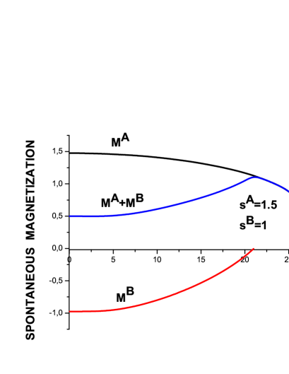
fluctuations of the and spins (II). As a result the magnons’ fluctuations suppress in a different way the magnetization on sublattices and . Quantitatively this depends on the coefficients and . At characteristic temperature spontaneous magnetization on sublattice becomes equal to zero, while spontaneous magnetization on sublattice is still nonzero (see Fig.1).
To study the magnetic properties of the system above we first consider the paramagnetic phase. To this end we make use of the Takahashi modified spin-wave theory Takahashi87 and introduce two parameters and to enforce the magnetization on the two sublattices to be equal to zero. The new Hamiltonian is obtained from the old one equation (1) by adding two new terms:
(14)
In momentum space the new Hamiltonian adopts the form Eq.(4) with new dispersions
(15)
Utilizing the same transformation (II) one obtains the Hamiltonian in diagonal form (7) with dispersions and obtained from Eqs.(II) replacing and with and respectively.
It is convenient to represent the parameters
and in the form
(16)
The dispersions and
are positive for all values of the wavevector , if the parameters and are positive.
The dispersions and are well defined if
(17)
The excitation is gapped ()
for all values of parameters and which satisfy equation (17). The excitation is gapped if , but in the particular case
(18)
, and near the zero wavevector . Therefor, in the particular case Eq. (18) boson is the long-range excitation (magnon) in the system.
Above Néel temperature we introduced the parameters and () to enforce the sublattice and spontaneous magnetizations to be equal to zero. We find out these and Hartree-Fock parameters, as functions of temperature, solving the system of five equations, equations (11) and the equations , where the spontaneous magnetization has the same representation as equations (13) but with coefficients , and dispersions in the expressions for the Bose functions.
The numerical calculations show that above Néel temperature
. When the temperature decreases the product decreases, remaining larger than one. The temperature at which the product becomes equal to one () is the Néel temperature Fig.(6).
Below , the spectrum contains long-range (magnon) excitations. Thereupon, and one can use the representation
. Then, and Hartree-Fock parameters are solution of a system of four equations, equations (11) and the equation .
We utilize the
obtained functions , , , (see Appendix C) to calculate the spontaneous magnetization as a function of the temperature. For a system with , , and the functions , and are depicted in figure (1).
Figure 1: (Color online) Spontaneous magnetization , and as a function of the temperature in units of exchange constant for ferrimagnetic spinel on bcc lattice with , , and . The partial order transition temperature is the temperature above which .
The partial order transition temperature is the temperature above which .
The customary formula for the entropy of a Bose system with Hamiltonian (7) is
(19)
where stays for and . The dispersions and (II) are used to define the Bose functions and below , dispersions and with are used for partial order phase , and with for paramagnetic phase above Néel temperature.
With entropy, as a function of temperature in mind, one can calculate the contribution of magnons to the specific heat:
(20)
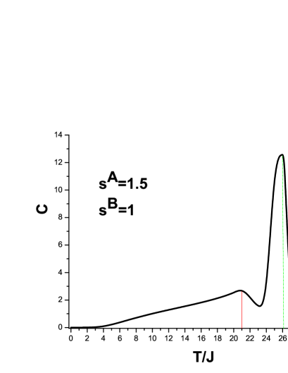
The resultant curve , for a system with the same parameters, as above, is depicted in figure (4).
Figure 2: (Color online) Specific heat vs temperature, in units of the exchange constant ,
for , , and . The high temperature (green) vertical line marks Néel temperature, while the low temperature (red) line marks partial order transition temperature .
The figures (1) and (2) show that the present method of calculation describes correctly the features of the system, partial order transition and anomalous behavior of the specific heat at the temperature of this transition .
III FC spinel ferrimagnetics
FC spinel ferrimagnetics are prepared applying magnetic field along the sublattice A magnetization upon cooling the material. This compensates the Zeeman splitting of sublattice B electrons which effectively leads to decrease of the spin. The Hamiltonian of the FC spinel ferrimagnet is
given by Eq.(1) with a varying parameter. The advantage of the method of calculation, presented above, is that we can use the same systems of equations for the three phases, , , , and different values of the parameter . We calculate the magnetization-temperature curves and the specific heat as a function of temperature for and three different values of (, and ), thus accounting for the increasing of the applied, during preparation of FC spinel, magnetic field.
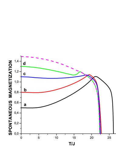
The resultant magnetization-temperature curves are depicted in figure (3).
Figure 3: Color online) Spontaneous magnetization as a function of the temperature in units of the exchange constant for ferrimagnetic spinel on bcc lattice with , , and :a)(black) , b)(red) , c)(blue) and d)(green) . The dash (magenta) line shows the spontaneous magnetization of sublattice for and .
The curve ”a” corresponds to ZFC spinel (see figure (1)). The increasing of the applied, during the preparation, magnetic field is modeled by decreasing of . The curves ”b”, ”c” and ”d” are magnetization-temperature curves for FC spinel ferrimagnetics with , and . The curve ”c” agrees well with the observed magnetization-temperature curve of FC spinel with an external magnetic field as high as 300 Oë applied upon cooling the material spinel08 ; spinel++ . The dash line shows the spontaneous magnetization of sublattice for and . Comparing with line ”d”, which shows the spontaneous magnetization of the same system one can conclude that contribution of the sublattice B magnetization is small and Zeeman splitting, of sublattice B electrons, is approximately compensated.
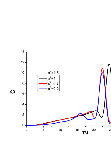
The dependence of specific heat on temperature for different values of is shown in figure (4).
Figure 4: (Color online) Specific heat vs temperature, in units of the exchange constant , for and different values of the effective spin : black curve , red curve and blue curve .
The curve with higher maximum corresponds to ZFC spinel (see figure (2))
With increasing the applied, during the preparation, magnetic field (with decreasing ) the anomalous temperature behavior of specific heat, at temperature of partial order transition, remains well defined but the pick decreases. The anomalous pick is well observed experimentally spinelCv1 ; spinel11b ; spinel12a , and one can use it to determine the temperature of the partial order transition.
IV Summary
In this paper is pointed out that a model which agrees well with the observed magnetic and thermodynamic properties of ZFC and FC spinel ferrimagnets is a two-sublattice Heisenberg model with spin- operators at the sublattice site, spin- operators at the sublattice site, ferromagnetic intra-sublattice exchange and antiferromagnetic inter-sublattice exchange. The applied magnetic field, along the sublattice A magnetization upon cooling the material, is accounted for varying only one parameter .
The subtle point is that spinel has an obvious anomalous magnetic behavior, but the appearance of this anomaly is attributed to the strong orbital-spin coupling spinel08 which is not discussed in the model (1). The spinel is a two-sublattice ferrimagnet, with site occupied by the ion, which is in the high-spin configuration with quenched orbital angular momentum, which can be regarded as a spin. The B site is occupied by the ion, which takes the high-spin configuration in the triply degenerate orbital and has orbital degrees of freedom. Because of the strong spin-orbital interaction it is convenient to consider coupling with and . The sublattice total angular momentum is , while the sublattice total angular momentum is , with , and spinel+ .
Then the g-factor for the sublattice is , and for the sublattice . The sublattice magnetic order is antiparallel to the sublattice one and the saturated magnetization is , in agreement with the experimental finding for ZFC spinel that the magnetization goes to zero when the temperature approaches zero.
The Hamiltonian of the system is
(21)
The first two terms describe the ferromagnetic Heisenberg intra-sublattice
exchange , while the third term describes the inter-sublattice exchange which is antiferromagnetic .
The operators and satisfy the algebra, therefor we can use the Holstein-Primakoff representation of the total angular momentum vectors and , where
and are Bose fields. Farther on, we repeat the calculations from sections II and III. The only difference is the expression for the magnetization . The model shows that the anomalous magnetic and thermodynamic behavior of is a consequence of the ferrimagnetic nature of the system.
Appendix A Spin-fermion model of spinel ferrimagnet
The Hamiltonian of the spin-fermion model of ferrimagnetic spinel defined on a body centered cubic lattice is
where , with the Pauli
matrices , is the spin of the itinerant
electrons at the sublattice site , is the spin of the localized electrons at the sublattice site,
is the chemical potential, and . The
sums are over all sites of a body centered cubic lattice, denotes the sum over the nearest neighbors, while and are sums over all sites of sublattice and respectively. The Heisenberg term describes ferromagnetic Heisenberg
exchange between localized electrons and is the antiferromagnetic exchange constant between localized and itinerant electrons. is the Zeeman splitting energy due to the external magnetic field (magnetic field in units of energy). We represent the Fermi operators, the spin of the itinerant electrons and the density operators in terms of the Schwinger bosons
() and slave fermions
(). The Bose fields
are doublets without charge, while fermions
are spinless with charges 1 () and -1 ():
(23)
(24)
To solve the constraint (Eq.24), one makes a change of variables, introducing
Bose doublets and
Schmeltzer
(25)
where the new fields satisfy the constraint
. In terms of the new fields
the spin vectors of the itinerant electrons have the form
(26)
When, in the ground state,
the lattice site is empty, the operator identity is
true. When the lattice site is doubly occupied, . Hence,
when the lattice site is empty or doubly occupied the spin on this
site is zero. When the lattice site is neither empty nor doubly
occupied (), the spin equals where the unit vector
(27)
identifies the local orientation of the spin of the
itinerant electron.
The part of Hamiltonian Eq.(A) with itinerant fermions can be rewritten in terms of Bose fields Eq.(A) and slave fermions
An important advantage of working with Schwinger bosons and slave fermions
is the fact that Hubbard term is in a diagonal form. The fermion-fermion and fermion-boson interactions are included in the hopping term. One treats them as a perturbation. To proceed we approximate the hopping term of the Hamiltonian Eq.(A) setting and keeping only the quadratic, with respect to fermions, terms. This means that the averaging in the subspace of the fermions is performed in one fermion-loop approximation. Further, we represent the resulting and Hamiltonian as a sum of two terms
(32)
where
is the Hamiltonian of the free and fermions, and
is the Hamiltonian of boson-fermion interaction.
The ground state of the system, without accounting for the spin fluctuations, is determined by the free-fermion Hamiltonian and is labeled by the density of electrons
(35)
(see equation (A)) and the ”effective spin” of the sublattice B electron
(36)
At half-filling
(37)
To solve this equation one sets the chemical potential . Utilizing this representation of we calculate the effective spin as a function of applied magnetic field for parameters and .
The result is depicted in figure (5).
Figure 5: (Color online) Sublattice B effective spin as a function of applied magnetic field for parameters and .
Let us introduce the vector,
(38)
Then, the spin-vector of itinerant electrons Eq.(26) can be written in the
form
(39)
where the vector identifies the local orientation of the spin of
the sublattice B itinerant electrons.
The Hamiltonian is quadratic with
respect to the fermions and , and one can
average in the subspace of these fermions (to integrate them out in
the path integral approach). As a result, accounting for the definition of (see
Eq.36), one obtains and an effective
model for spin vectors with Hamiltonian
(40)
where the effective exchange constant is calculated in the one loop approximation. The term with exchange constant in equation (A) and the mixed, spin-fermion term (30), adopt the form
(41)
and
(42)
respectively. Collecting all terms one obtains the Hamiltonian of the FC ferrimagnetic spinel
where and depending on the field applied during preparation Fig.(5). After the process of preparation the external magnetic field is set equal to zero. For systems with , discussed in the paper, one has to consider two-band model for sublattice B fermions. The result remains the same even for this more complicate system: the effective spin decreases when the applied, under the preparation, magnetic field increases.
Appendix B Hartree-Fock approximation
Let us consider a theory with Hamiltonian (1). We introduce Holstein-Primakoff representation for the spin
operators
(43)
when the sites are from sublattice and
(44)
when the sites are from sublattice . The operators and satisfy the Bose commutation relations. In terms of the Bose operators and keeping only the quadratic and quartic terms, the effective Hamiltonian
Eq.(1) adopts the form
(45)
where
The next step is to represent the Hamiltonian in the Hartree-Fock approximation (2,3) and
It is convenient to rewrite the Hamiltonian in momentum space representation Eq.(4)
The two equivalent sublattices A and B of the bcc lattice are simple cubic lattices. The wave vector runs over the reduced first Brillouin zone of a
bcc lattice which is the first Brillouin zone of a simple cubic lattice. The dispersions are given by equalities Eqs. (II)
To diagonalize the Hamiltonian one introduces new Bose fields
by means of the
transformation (II)
where the coefficients of the transformation and are real function of the wave vector
(49)
The transformed Hamiltonian adopts the form Eqs.(7)
with dispersions Eqs.(II)
The free energy of a system with Hamiltonian (7,II) is Eq.(II)
The system of equations for the Hartree-Fock parameters Eqs.(11),
in terms of the Bose functions of the and excitations, adopt the form
where and are the Bose functions of and excitations.
Appendix C Takahashi modified spin-wave theory Takahashi87
To study the paramagnetic phase of the system we make use of the Takahashi modified spin-wave theory Takahashi87 and introduce two parameters and to enforce the magnetization on the two sublattices to be equal to zero. It is convenient to represent the parameters
and in the form Eqs.(16).
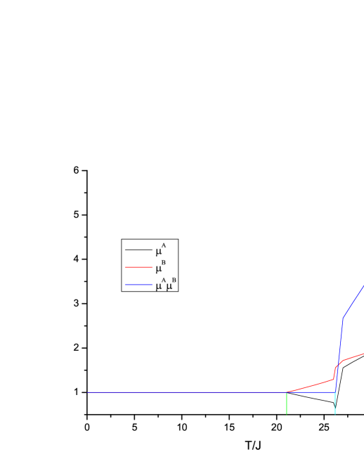
We find out these and Hartree-Fock parameters, as functions of temperature, solving the system of five equations, equations (B) and the equations . The numerical calculations show that above Néel temperature (blue line in Fig.(6)). When the temperature decreases the product decreases, remaining larger than one. The temperature at which the product becomes equal to one () is the Néel temperature, marked by vertical cyan line in Fig.(6).
At low temperature and (). The Hartree-Fock parameters are positive functions of , solution of the system of equations (B). Utilizing these functions, one can calculate the spontaneous magnetization on the two sublattices at low temperature. At characteristic temperature spontaneous magnetization on sublattice becomes equal to zero, while spontaneous magnetization on sublattice is still nonzero (see Fig.1 in the paper).
Above the spectrum contains long-range (magnon) excitations. Thereupon, and one can use the representation
. Then, and Hartree-Fock parameters are solution of a system of four equations, equations (B) and the equation .
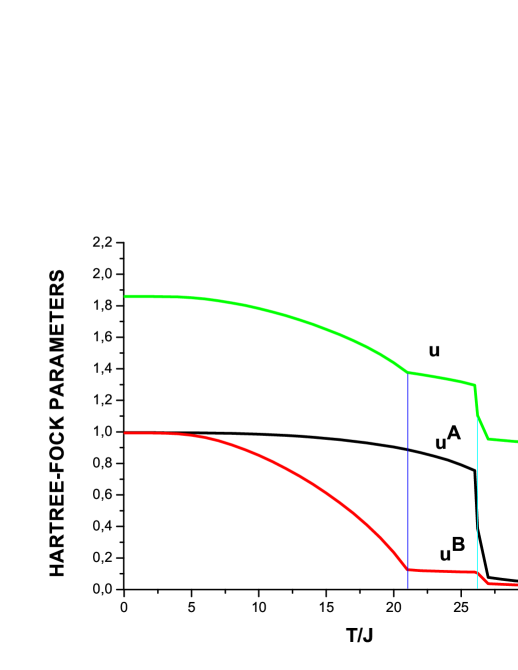
The functions , and are depicted in figure (6) for a system with , , and .
For the same system the Hartree-Fock parameters , are depicted in figure (7).
Figure 6: (Color online) Parameters , and as a function of the temperature, in units of the exchange constant , for ferrimagnet with sublattice A spin and sublattice B spin . The high temperature vertical (cyan) line corresponds to the Néel temperature of ferrimagnet to paramagnet transition. The low temperature vertical (green) line corresponds to partial order transition temperature.
Figure 7: (Color online) Hartree-Fock parameters as a function of the temperature, in units of the exchange constant , for ferrimagnet with sublattice A spin and sublattice B spin . The high temperature vertical (cyan) line marks the Néel temperature of ferrimagnet to paramagnet transition. The low temperature vertical (blue) line marks the partial order transition temperature.
References
(1) K. Adachi, T. Suzuki, K. Kato, K. Osaka, M. Takata and T. Katsufuji, Phys. Rev. Lett. 95, 197202 (2005).
(2) Zhaorong Yang, Shun Tan, Zhiwen Chen, and Yuheng Zhang, Phys. Rev. B 62, 13872 (2000).
(3) H. D. Zhou, J. Lu, and C. R. Wiebe, Phys. Rev. B 76, 174403 (2007).
(4) V. O. Garlea, R. Jin, D. Mandrus, B. Roessli, Q. Huang, M. Miller, A. J. Schultz, and S. E. Nagler, Phys. Rev. Lett. 100, 066404 (2008).
(5) S-H. Baek, K-Y. Choi, A. P. Reyes, P. L. Kuhns, N. J. Curro, V. Ramanchandran, N. S. Dalal, H. D. Zhou, and C. R. Wiebe,
J. Phys.: Condens. Matter 20, 135218 (2008).
(6) Kim Myung-Whun, J. S. Kim, T. Katsufuji, and R. K. Kremer, Phys. Rev. B 83, 024403 (20011).
(7) A. Kiswandhi, J. S. Brooks, J. Lu, J. Whalen, T. Siegrist, and H. D. Zhou, Phys. Rev. B 84, 205138 (2011).
(8) A. Kismarahardja, J. S. Brooks, A. Kiswandhi, K. Matsubayashi, R. Yamanaka, Y. Uwatoko, J. Whalen,
T. Siegrist, and H. D. Zhou, Phys. Rev. Lett. 106, 056602 (2011).
(9)Q. Zhang, K. Singh, F. Guillou, C. Simon, Y. Breard, V. Caignaert, and V. Hardy, Phys. Rev. B 85, 054405 (2012).
(10) Y. Nii, H. Sagayama, T. Arima, S. Aoyagi, R. Sakai, S. Maki, E. Nishibori, H. Sawa, K. Sugimoto,
H. Ohsumi, and M. Takata, Phys. Rev. B 86, 125142 (2012).
(11) Z. H. Huang, X. Luo, S. Lin, Y. N. Huang, L. Hu, L. Zhang, Y. P.Sun, Solid State Communications 159, 88 (2013).
(12) Z. H. Huang, X. Luo, L. Hu, S. G. Tan, Y. Liu, B. Yuan, J. Chen, W. H. Song, and Y. P. Sun, Journal of Applied Physics 115, 034903 (2014).
(13) Dina Tobia, Julin Milano, Maria Teresa Causa and Elin L. Winkler,
J. Phys.: Condens. Matter 27, 016003 (2015).
(14) Vincent Hardy, Yohann Brard, and Christine Martin, Phys. Rev. B 78, 024406 (2008).
(15) R. Quartu and H. T. Diep, Phys. Rev. B 55, 2975 (1997).
(16) J. R. Stewart, G. Ehlers, A. S. Wills, S. T. Bramwell, and J. S. Gardner, J. Phys.: Condens. Matter 16, L321
(2004).
(17) P. Azaria, H. T. Diep, and H. Giacomini, Phys. Rev. Lett. 59, 1629 (1987).
(18) V. G. Vaks, A. I. Larkin, and Y. N. Ovchinnikov, JETP Letters. 22, 820 (1966).
(19) H. T. Diep, Ed., Frustrated Spin Systems, World Scientific (2004)
(20) M. Takahashi, Phys. Rev. Lett. 58, 168 (1987).