Why GPS makes distances bigger than they are

Peter Ranacher ^1∗, Richard Brunauer², Wolfgang Trutschnig ³ Stefan Christiaan Van der Spek⁴, and Siegfried Reich ²

1 Department of Geoinformatics - Z_GIS, University of Salzburg, Schillerstraße 30, 5020 Salzburg, Austria

2 Salzburg Research Forschungsgesellschaft mbH, Jakob Haringer Straße 5/3, 5020 Salzburg, Austria

3 Department of Mathematics, University of Salzburg, Hellbrunner Straße 34, 5020 Salzburg, Austria

4 Delft University of Technology, Faculty of Architecture, Department of Urbanism, Julianalaan 134, 2628BL Delft, The Netherlands

Abstract

Global Navigation Satellite Systems (GNSS), such as the Global Positioning System (GPS), are among the most important sensors for movement analysis. GPS is widely used to record the trajectories of vehicles, animals and human beings. However, all GPS movement data are affected by both measurement and interpolation error. In this article we show that measurement error causes a systematic bias in distances recorded with a GPS: the distance between two points recorded with a GPS is – on average – bigger than the true distance between these points. This systematic ‘overestimation of distance’ becomes relevant if the influence of interpolation error can be neglected, which is the case for movement sampled at high frequencies. We provide a mathematical explanation of this phenomenon and we illustrate that it functionally depends on the autocorrelation of GPS measurement error ($C$). We argue that $C$ can be interpreted as a quality measure for movement data recorded with a GPS. If there is strong autocorrelation any two consecutive position estimates have very similar error. This error cancels out when average speed, distance or direction are calculated along the trajectory.

Based on our theoretical findings we introduce a novel approach to determine $C$ in real-world GPS movement data sampled at high frequencies. We apply our approach to a set of pedestrian and a set of car trajectories. We find that the measurement error in the data is strongly spatially and temporally autocorrelated and give a quality estimate of the data. Finally, we want to emphasize that all our findings are not limited to GPS alone. The systematic bias and all its implications are bound to occur in any movement data collected with absolute positioning if interpolation error can be neglected.

1 Introduction

Global Navigation Satellite Systems (GNSSs), such as the Global Positioning System (GPS), have become essential sensors for collecting the movement of objects in geographical space. In movement ecology, GPS tracking is used to unveil the migratory paths of birds (Higuchi and Pierre, 2005), elephants (Douglas-Hamilton et al., 2005) or roe deer (Andrienko et al., 2011). In urban studies, GPS movement data help detecting traffic flows (Zheng et al., 2011) and human activity patterns in cities (Van der Spek et al., 2009). In transportation research, GPS allows monitoring of intelligent vehicles (Zito et al., 1995) and mapping of transportation networks (Mintsis et al., 2004), to name but a few application examples.

Movement recorded with a GPS is commonly stored in form of a trajectory. A trajectory $\tau$ is an ordered sequence of spatio-temporal positions: $\tau={<(\boldsymbol{P_{1}},t_{1}),...,(\boldsymbol{P_{n}},t_{n})>}$, with $t_{1}<...<t_{n}$ (Güting and Schneider, 2005). The tuple $(\boldsymbol{P},t)$ indicates that the moving object was at a position $\boldsymbol{P}$ at time $t$. In order to represent the continuity of movement, consecutive positions $(\boldsymbol{P_{i}},t_{i})$ and $(\boldsymbol{P_{j}},t_{j})$ along the trajectory are connected by an interpolation function (Macedo et al., 2008).

However, although satellite navigation provides global positioning at an unprecedented accuracy, GPS trajectories remain affected by errors. There are two types of error inherent in any kind of movement data, measurement error and interpolation error (Schneider, 1999), and these errors inevitably also affect trajectories recorded with a GPS.

• Measurement error refers to the impossibility of determining the actual position $(\boldsymbol{P},t)$ of an object due to the limitations of the measurement system. In the case of satellite navigation, it reflects the spatial uncertainty associated with each position estimate.

• Interpolation error refers to the limitations on interpolation representing the actual motion between consecutive positions $(\boldsymbol{P_{i}},t_{i})$ and $(\boldsymbol{P_{j}},t_{j})$. This error is influenced by the temporal sampling rate at which a GPS records the positions.

Measurement and interpolation errors cause the movement recorded with a GPS to differ from the actual movement of the object. This needs to be taken into account in order to achieve meaningful results from GPS data.

In this article we focus on GPS measurement error in movement data. We show that measurement error causes a systematic overestimation of distance. Distances recorded with a GPS are – on average – always bigger than the true distances travelled by a moving object, if the influence of interpolation error can be neglected. In practice, this is the case for movement recorded at high frequencies. We provide a rigorous mathematical explanation of this phenomenon. Moreover, we show that the overestimation of distance is functionally related to the spatio-temporal autocorrelation of GPS measurement error. We build on this relationship and provide a novel methodology to assess the quality of GPS movement data. Finally we demonstrate our method on two types of movement data, namely the trajectories of pedestrians and cars.

Section 2 introduces relevant work from previously published literature. Section 3 provides a mathematical explanation of why GPS measurement error causes a systematic overestimation of distance. Section 4 shows how this overestimation can be used to reason about the spatio-temporal auto-correlation of measurement error. Section 5 describes the experiment and presents our experimental results, section 6 discusses the results.

2 Related work

Since GPS data have become a common component of scientific analyses its quality parameters have received considerable attention. These parameters include the accuracy of the estimated position, the availability and the update rate of the GPS signal, as well as the continuity, integrity, reliability and coverage of the service (Hofmann-Wellenhof et al., 2003). The accuracy of the estimated position (i.e. the expected conformance of a position provided with a GPS to the true position, or the anticipated measurement error) is clearly of utmost importance. Measurement error and its causes, influencing factors, and scale have been extensively discussed in published literature: measurement error has been shown to vary over time (Olynik, 2002) and to be location-dependent. Shadowing effects, for example due to canopy cover, have a significant influence on its magnitude (D’Eon et al., 2002). Measurement error is both random and caused by external influences, as well as systematic and caused by the system’s limitations (Parent et al., 2013).

Measurement error is the result of several influencing factors. According to Langley (1997), these include:

• Propagation delay: atmospheric variations can affect the speed of the GPS signal and hence the time that it takes to reach the receiver;

• drift in the GPS clock: a drift in the on-board clocks of the different GPS satellites causes them to run asynchronously with respect to each other and to a reference clock;

• Ephemeris error: imprecise satellite data and incorrect physical models affect estimations of the true orbital position of each GPS satellite (Colombo, 1986);

• Hardware error: the GPS receiver, being as fault-prone as any other measurement instrument, produces an error when processing the GPS signal;

• Multipath propagation: infrastructure close to the receiver can reflect the GPS signal and thus prolong its travel time from the satellite to the receiver;

• Satellite geometry: an unfavourable geometric constellation of the satellites reduces the accuracy of positioning results.

There are several quality measures to describe GPS measurement error, the most common being the 95 $\%$ radius ($R95$), which is defined as the radius of the smallest circle that encompasses 95 $\%$ of all position estimates (Chin, 1987). The official GPS Performance Analysis Report for the Federal Aviation Administration issued by the William J. Hughes Technical Center (2013) states that the current set-up of the GPS allows to measure a spatial position with an average $R95$ of slightly over 3 meters using the Standard Positioning Service (SPS). The values in the report were, however, obtained from reference stations that were equipped with high quality receivers and had unobstructed views of the sky. It is reasonable to assume that the accuracy would be reduced in other recording environments, as measurement error depends to a considerable extent on the receiver, as well as on the geographic location (William J. Hughes Technical Center, 2013; Langley, 1997). This assumption is supported by published literature on GPS accuracy in forests (Sigrist et al., 1999) and on urban road networks (Modsching et al., 2006), as well as on the accuracies of different GPS receivers (Wing et al., 2005; Zandbergen, 2009). On the other hand, the accuracy of GPS can be increased using differential global positioning systems (DGPS) such as the European Geostationary Navigation Overlay Service (EGNOS). DGPS estimate and correct the propagation delay in the ionosphere, thus yielding higher position accuracies (Hofmann-Wellenhof et al., 2003).

A detailed overview of current GPS accuracy is provided in the quarterly GPS Performance Analysis Report for the Federal Aviation Administration. A good introduction to the GPS in general, and to its error sources and quality parameters in particular, has been provided by Hofmann-Wellenhof et al. (2003).

The above-mentioned research has mainly focused on describing and understanding GPS measurement error. In addition to this, filtering and smoothing approaches have been proposed for recording movement data, in order to reduce the influence of errors on movement trajectories. A concise summary of these approaches can be found in Parent et al. (2013). Jun et al. (2006) tested smoothing methods that best preserve travelled distance, speed, and acceleration. The authors found that Kalman filtering resulted in the least difference between the true movement and its representation.

3 GPS measurement error causes a systematic overestimation of distance

A GPS measurement consists of a spatial component (i.e. latitude $\phi$, longitude $\lambda$) and a temporal component (i.e. a time stamp $t$). In this article we will mainly focus on the spatial component.

The GPS uses the World Geodetic System 1984 (WGS84) as a coordinate reference system. For reasons of simplicity it is preferable to transform the GPS measurements to a Cartesian map projection, such as the Universal Transversal Mercator (UTM). A transformation from an ellipsoid (WGS84) to a Cartesian plane (UTM) leads to a distortion of the original trajectories (Hofmann-Wellenhof et al., 2003). For vehicle, pedestrian, or animal movements consecutive positions along a trajectory are usually sampled in intervals ranging from seconds to minutes. Thus, these positions are very close together in space so that the distortion is insignificant for most practical applications. Hence, for all the following consideration we assume that the movement is recorded in UTM.

Very generally, a spatial position in UTM is a two-dimensional coordinate

$${\boldsymbol{P}}=\left(\begin{array}[]{c}x\\ y\\ \end{array}\right),$$ (1)

where $x$ is the metric distance of the position from a reference point in eastern direction and $y$ in northern direction. If a moving object is recorded at position ${\boldsymbol{P}}$ with a GPS, the position estimate $\boldsymbol{P^{m}}=(x^{m},y^{m})$ is affected by measurement error. The relationship between the true position and its estimate is very trivially

$$\boldsymbol{P^{m}}=\boldsymbol{P}+\boldsymbol{{\varepsilon_{P}}}\text{,}$$ (2)

where $\boldsymbol{{\varepsilon_{P}}}$ is the horizontal measurement error expressed as a vector in the horizontal plane. $\boldsymbol{{\varepsilon_{P}}}$ is drawn from $\boldsymbol{{\mathcal{E}_{P}}}$, the distribution of measurement error at $\boldsymbol{{P}}$. We adopt the convention used by Codling et al. (2008) to denote random variables with upper case letters and their numerical values with lower case letters.

We now provide a detailed mathematical explanation of why measurement error causes a systematic overestimation of distance in trajectories, if interpolation error can be neglected. Figure 1 illustrates the problem statement in a simplified form. Consider a moving object equipped with a GPS. The moving object travels between two arbitrary positions $\boldsymbol{P}$ and $\boldsymbol{Q}$. Let $d_{0}=d(\boldsymbol{P},\boldsymbol{Q})$ denote the Euclidean distance between these, henceforth referred to as reference distance. The object always moves along a straight line, consequently interpolation error can be neglected. The movement of the object can be described by the following five steps, which correspond to the subplots in Figure 1.

1. The moving object starts at $\boldsymbol{P}$. The GPS obtains the position estimate $\boldsymbol{P^{m}}$ with measurement error $\boldsymbol{{\varepsilon_{P}}}$, which is drawn from $\boldsymbol{{\mathcal{E}_{P}}}$.

2. The moving object travels to $\boldsymbol{Q}$. The GPS obtains the position estimate $\boldsymbol{Q^{m}}$ with measurement error $\boldsymbol{{\varepsilon_{Q}}}$, which is drawn from $\boldsymbol{{\mathcal{E}_{Q}}}$. The distance between the two position estimates is calculated: ${d^{m}}=d(\boldsymbol{P^{m}},\boldsymbol{Q^{m}})$.

3. The moving object returns to $\boldsymbol{P}$. The GPS obtains a position estimate and a new ${d^{m}}$ is calculated.

4. Steps 2 and 3 are repeated $n$ times, where $n$ is an infinitely large number.

5. After $n$ repetitions, the position estimates scatter around $\boldsymbol{P}$ and $\boldsymbol{Q}$ with measurement error $\boldsymbol{{\mathcal{E}_{P}}}$ and $\boldsymbol{{\mathcal{E}_{Q}}}$.

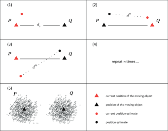
Figure 1: A moving object equipped with a GPS travels between two arbitrary positions

We claim that measurement error propagates to the expected measured distance $\mathbb{E}(d^{m})$ and to the expected squared measured distance $\mathbb{E}(d_{2}^{m})$ between the position estimates. More specifically, measurement error yields $\mathbb{E}(d^{m})>d_{0}$ as well as $\mathbb{E}(d_{2}^{m})>d_{0}^{2}$.

We are now going to rigorously prove this claim. To do so, we simplify notation, write $\boldsymbol{{\mathcal{E}_{P}}}=(X_{1},Y_{1})$ as well as $\boldsymbol{{\mathcal{E}_{Q}}}=(X_{2},Y_{2})$, and assume that there is no systematic bias, i.e. we have $\mathbb{E}(X_{1})=\mathbb{E}(X_{2})=\mathbb{E}(Y_{1})=\mathbb{E}(Y_{2})=0$. Since neither translations nor rotations affect distances between points we may, without loss of generality, consider $\boldsymbol{P}=(0,0)$ and $\boldsymbol{Q}=(d_{0},0)$. Since linear transformations (like rotations) preserve expectation, rotating errors with expectation zero results in errors having expectation zero too. Having this we can now formulate the following first result for the expected squared distance $\mathbb{E}(d^{2}(\boldsymbol{P^{m}},\boldsymbol{Q^{m}}))$. For mathematical background we refer to Klenke (2013). Notice that no assumptions (like absolute continuity or normality) about the underlying error distributions are needed, i.e. the result holds in full generality.

Theorem 1

Suppose that $d_{0}>0$, that $\boldsymbol{P}=(0,0)$, and that $\boldsymbol{Q}=(d_{0},0)$. Let $X_{1},X_{2}$ both have distribution function $F$ and variance $\sigma_{X}^{2}$, and $Y_{1},Y_{2}$ both have distribution function $G$ and variance $\sigma_{Y}^{2}$. Furthermore assume that $\mathbb{E}(X_{1})=\mathbb{E}(X_{2})=\mathbb{E}(Y_{1})=\mathbb{E}(Y_{2})=0$. Then the following two conditions are equivalent:

1. $\mathbb{E}(d_{2}^{m})=\mathbb{E}(d^{2}(\boldsymbol{P^{m}},\boldsymbol{Q^{m}}))>d_{0}^{2}$

2. $\min\{Cov(X_{1},X_{2}),Cov(Y_{1},Y_{2})\}<1$

In other words: the expected squared distance $\mathbb{E}(d_{2}^{m})$ is strictly greater than $d_{0}^{2}$ unless the errors fulfil $X_{1}=X_{2}$ and $Y_{1}=Y_{2}$ with probability one (which describes the situation of always having identical errors in $\boldsymbol{P}$ and $\boldsymbol{Q}$).

Proof: Calculating $\mathbb{E}(d^{2}(\boldsymbol{P^{m}},\boldsymbol{Q^{m}}))$ and using the fact that $\textit{Cov}(X_{1},X_{2})\leq\sigma_{X}^{2}$ and $\textit{Cov}(Y_{1},Y_{2})\leq\sigma_{Y}^{2}$ directly yields

$$\mathbb{E}(d^{2}(\boldsymbol{P^{m}},\boldsymbol{Q^{m}})) = \mathbb{E}(d_{0}+X_{2}-X_{1})^{2}+\mathbb{E}(Y_{2}-Y_{1})^{2}$$

$$= d_{0}^{2}+\mathbb{E}(X_{2}-X_{1})^{2}+\mathbb{E}(Y_{2}-Y_{1})^{2}=d_{0}^{2}+\textit{Var}(X_{2}-X_{1})+\textit{Var}(Y_{2}-Y_{1})$$

$$= d_{0}^{2}+2\sigma_{X}^{2}+2\sigma_{Y}^{2}-2\textit{Cov}(X_{1},X_{2})-2\textit{Cov}(Y_{1},Y_{2})$$

$$\geq d_{0}^{2}.$$

Having this it follows immediately that $\mathbb{E}(d^{2}(\boldsymbol{P^{m}},\boldsymbol{Q^{m}}))=d_{0}^{2}$ if and only if $\textit{Cov}(X_{1},X_{2})=\sigma_{X}^{2}$ and $\textit{Cov}(Y_{1},Y_{2})=\sigma_{Y}^{2}$, which in turn is equivalent to the fact that $X_{1}=X_{2}$ and $Y_{1}=Y_{2}$ holds with probability one. $\blacksquare$

In general one is, however, interested in the expected distance $\mathbb{E}(d^{m}):=\mathbb{E}(d(\boldsymbol{P^{m}},\boldsymbol{Q^{m}}))$ and not in the expected squared distance. Since, in general, $\mathbb{E}(Z^{2})>d_{0}^{2}$ need not imply $\mathbb{E}(|Z|)>d_{0}$ for arbitrary random variables $Z$, a different method is used to prove the following main result:

Theorem 2

Suppose that the assumptions of Theorem 1 hold. Then the following two conditions are equivalent:

1. $\mathbb{E}(d^{m})=\mathbb{E}(d(\boldsymbol{P^{m}},\boldsymbol{Q^{m}}))>d_{0}$

2. $\max\big{\{}\mathbb{P}(Y_{1}\not=Y_{2}),\mathbb{P}(X_{2}-X_{1}<-d_{0})\big{\}}>0$

In other words: the expected distance $\mathbb{E}(d^{m})$ is strictly greater than the true distance $d_{0}$ unless the errors fulfil $Y_{1}=Y_{2}$ with probability one and $\mathbb{P}(X_{2}-X_{1}<-d_{0})=0$ holds.

Proof: Obviously we have

$$\sqrt{(d_{0}+X_{2}-X_{1})^{2}+(Y_{2}-Y_{1})^{2}}\geq|d_{0}+X_{2}-X_{1}|$$ (4)

Setting $Z:=X_{2}-X_{1}$ implies $\mathbb{E}(Z)=0$. Assume now that $\mathbb{P}(Z<-d_{0})>0$ holds. Then the desired inequality follows immediately from

$$\mathbb{E}|Z+d_{0}| = \int_{\mathbb{R}}|z+d_{0}|\,d\mathbb{P}^{Z}=\int_{[-d_{0},\infty]}(z+d_{0})\,d\mathbb{P}^{Z}+\int_{(-\infty,-d_{0})}-(z+d_{0})\,d\mathbb{P}^{Z}$$

$$= \underbrace{\int_{\mathbb{R}}(z+d_{0})\,d\mathbb{P}^{Z}}_{=d_{0}}\,+\,\,\underbrace{(-2)\int_{(-\infty,-d_{0})}(z+d_{0})\,d\mathbb{P}^{Z}}_{>0}$$

$$> d_{0}.$$

In case we have $\mathbb{P}(Z<-d_{0})=0$ but $\mathbb{P}(Y_{1}\not=Y_{2})>0$ holds, then Inequality 4 is strict with positive probability so we get

$$\mathbb{E}(d^{m})=\mathbb{E}\Big{(}\sqrt{(d_{0}+X_{2}-X_{1})^{2}+(Y_{2}-Y_{1})^{2}}\Big{)}>\mathbb{E}(|d_{0}+X_{2}-X_{1}|)=\mathbb{E}(|Z+d_{0}|)=d_{0}.$$

Altogether this shows that the second condition of Theorem 2 implies the first one.
To prove the reverse implication, assume that $\max\big{\{}\mathbb{P}(Y_{1}\not=Y_{2}),\mathbb{P}(X_{2}-X_{1}<-d_{0})\big{\}}=0$. Then, firstly, the left and the right hand-side of Inequality 4 coincide with probability one, so $\mathbb{E}(d^{m})=\mathbb{E}\big{(}\sqrt{(d_{0}+X_{2}-X_{1})^{2}+(Y_{2}-Y_{1})^{2}}\big{)}=\mathbb{E}(|d_{0}+X_{2}-X_{1}|)$ holds. And secondly, directly applying Equality 3 yields $\mathbb{E}(|Z+d_{0}|)=d_{0}$, which finally shows $\mathbb{E}(d^{m})=d_{0}$. $\blacksquare$

Remark 1

It is worth mentioning that Theorem 2 has several interesting (and partially surprising) consequences: Whenever the errors in $x$-direction are unbounded (like in the case of normal distributions) the expected distance is always strictly greater than the true distance $d_{0}$. The same holds whenever the errors $Y_{1}$ and $Y_{2}$ in $y$-direction do not always coincide – a very realistic assumption for GPS trajectories.

We want to underline that Theorem 1 and 2 hold in full generality for arbitrary distributions of GPS measurement error. Although GPS measurement error is often assumed to have a bivariate normal distribution and to be independent in both the $x$- and $y$-direction (Jerde and Visscher, 2005; Bos et al., 2008), Chin (1987) puts forward convincing arguments why this is very likely not the case. Hence, the general validity of our findings is relevant.

For reasons of simplicity, we have assumed that $\boldsymbol{{\mathcal{E}_{P}}}$ and $\boldsymbol{{\mathcal{E}_{Q}}}$ follow the same distribution function and that there is no systematic bias, i.e. $\boldsymbol{{\mathcal{E}_{P}}}$ is centred around $\boldsymbol{P}$ and $\boldsymbol{{\mathcal{E}_{Q}}}$ around $\boldsymbol{Q}$. This assumption is generally acknowledged for in the literature. It builds, for example, the basis for algorithms to extract road maps from GPS tracking data (e.g. Wang et al., 2014). Roads are assumed to be located where the density of the GPS measurements is the highest. Also Figure 4 shows that this assumption is indeed realistic for real-world GPS data. However, even a systematic bias does not necessary restrict the validity of our argument. Let us assume that $\mathbb{E}(X_{1})=\mathbb{E}(X_{2})\neq 0$ and $\mathbb{E}(Y_{1})=\mathbb{E}(Y_{2})\neq 0$, i.e. the mean of the error distribution has shifted away from $\boldsymbol{P}$ and $\boldsymbol{Q}$ respectively. As the shift is the same for $\boldsymbol{{\mathcal{E}_{P}}}$ and $\boldsymbol{{\mathcal{E}_{Q}}}$, the influence on distance calculations cancels out, Theorem 1 and 2 still hold. The validity of our proof is restricted only if $\mathbb{E}(X_{1})\neq\mathbb{E}(X_{2})$ or $\mathbb{E}(Y_{1})\neq\mathbb{E}(Y_{2})$. This implies that the mean of the error distribution changes abruptly between $\boldsymbol{P}$ and $\boldsymbol{Q}$. As – in practice – $\boldsymbol{P}$ and $\boldsymbol{Q}$ are very close in space, this scenario is not realistic for GPS measurement error.

4 How big is the overestimation of distance and why is this relevant?

In the previous Section we proved that distances recorded with a GPS are on average bigger than the distances travelled by a moving object, if interpolation error can be neglected. In this Section we provide an equation for OD, the expected overestimation of distance. Moreover, we identify three parameters that influence the magnitude of OD. First, let us define OD with the help of Equation 3:

$$\textit{OD}=\mathbb{E}(d^{m}_{2})^{\frac{1}{2}}-d_{0}=(d^{2}_{0}+2\sigma_{X}^{2}+2\sigma_{Y}^{2}-2\textit{Cov}(X_{1},X_{2})-2\textit{Cov}(Y_{1},Y_{2}))^{\frac{1}{2}}-d_{0}.$$

From this follows that OD is a function of three parameters:

1. $d_{0}$, the reference distance between $\boldsymbol{P}$ and $\boldsymbol{Q}$
   

2. $\textit{Var}_{\textit{gps}}=2\sigma_{X}^{2}+2\sigma_{Y}^{2}$, a term for the variance of GPS measurement error
   

3. $C=2\textit{Cov}(X_{1},X_{2})-2\textit{Cov}(Y_{1},Y_{2})$, a term for the auto-correlation of GPS measurement error. $C$ expresses the similarity of any two consecutive position estimates. If $C$ is big, consecutive position estimates are affected by similar GPS measurement error (see also Figure 2).

We can now simplify notation and write

$$\textit{OD}=(d^{2}_{0}+\textit{Var}_{\textit{gps}}-C)^{\frac{1}{2}}-d_{0}.$$ (6)

The influence of the three parameters on OD is further illustrated in Figure 2. OD is small if the reference distance is big, the variance of GPS measurement error is small and the error has high positive autocorrelation. OD is big if the reference distance is small, the variance of GPS measurement error is big and the error has high negative autocorrelation.

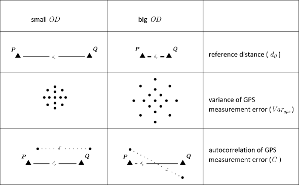
Figure 2: Overestimation of distance (OD) and its influencing parameters.

To understand the magnitude of OD in real-world GPS data, let us assume for a moment that there is no autocorrelation of GPS measurement error, i.e. $C=0$. Moreover, let us assume that the variance of error is the same in $x$- and $y$- directions, i.e. $\sigma^{2}=\sigma_{X}^{2}=\sigma_{Y}^{2}$ and $\textit{Var}_{\textit{gps}}=4\sigma^{2}$. We can now visualize the relationship between OD, $d_{0}$ and $\sigma$. Figure 3 a shows that $\mathit{OD}$ increases as the spread of GPS measurement error ($\sigma$) increases; $d_{0}$ is assumed to be constant. For a constant $d_{0}$ of $5{m}$, for example, and $\sigma=2\rm{m}$ the overestimation of distance roughly equals $2\rm{m}$ (yellow line). When $\sigma$ increases to $4\rm{m}$ the overestimation of distance increases to $4\rm{m}$. Figure 3 b shows that $\mathit{OD}$ decreases as $d_{0}$ increases; $\sigma$ is assumed to be constant. For a constant $\sigma$ of $3\rm{m}$, for example, and $d_{0}=5{m}$ the overestimation of distance equals around $3\rm{m}$ (black line). When $d_{0}$ increases to $10{m}$ the overestimation of distance decreases to $2\rm{m}$.

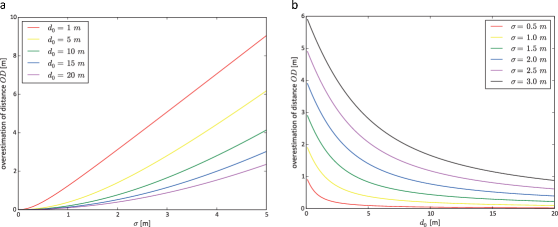
Figure 3: The overestimation of distance $(\mathit{OD}$) increases as the spread of GPS measurement error ($\sigma$) increases, the reference distance ($d_{0}$) is constant (a); $\mathit{OD}$ decreases as $d_{0}$ increases $\sigma$ is constant (b).

Remember that Figure 3 shows the influence of $\textit{Var}_{\textit{gps}}$ if there is no autocorrelation of GPS measurement error. This is not very realistic for real world GPS data. In fact, El-Rabbany and Kleusberg (2003); Wang et al. (2002) and Howind et al. (1999) show that GPS is affected by both spatial and temporal autocorrelation. This means that position estimates taken close in space and in time tend to have similar error.

How big is the autocorrelation of GPS measurement error? Let us reformulate Equation 6 and solve for $C$:

$$C=d_{0}^{2}-\overbrace{\textbullet(\textit{OD}+d_{0})^{2}}^{\mathbb{E}(d^{m}_{2})}+\textit{Var}_{\textit{gps}}.$$ (7)

This implies that we can calculate the autocorrelation of GPS measurement error if $\mathit{OD}$, $\textit{Var}_{\textit{gps}}$ and $d_{0}$ are known. Things become interesting if we consider what autocorrelation really means in the context of GPS positioning. In Figure 2, in the bottom left cell, the position estimates $\boldsymbol{P^{m}}$ and $\boldsymbol{Q^{m}}$ are highly auto-correlated and, hence, very similar. This leads to the effect that $d^{m}$ is very similar to $d_{0}$. In fact, this applies not only to distance, but to other movement parameters as well. Direction, speed, acceleration or turning angle must all be similar to the ‘true’ movement of the object if they are derived from highly auto-correlated GPS position estimates. Consequently, $C$ describes how well a GPS captures the movement of an object, if interpolation error can be neglected. Or in other words, $C$ is a quality measure for GPS movement data.

5 Assessing the quality of GPS movement data

Real world GPS data are affected by spatial as well as temporal autocorrelation (El-Rabbany and Kleusberg, 2003; Wang et al., 2002; Howind et al., 1999). Spatial autocorrelation implies that GPS measurement error is not independent of space. Measurements obtained at similar locations will have similar error. Temporal autocorrelation implies that GPS measurement error is not independent of time. Measurements obtained at similar times will have a similar error due to similar atmospheric conditions and a similar satellite constellation (Bos et al., 2008). We carried out a simple experiment to visualize temporal autocorrelation in real-world GPS data. We placed a GPS unit at a known position $\boldsymbol{P}$ and recorded about 720 position estimates over a period of about six hours at a sampling rate of $1/30~{}\mathrm{Hz}$. The resulting distribution is centred around $\boldsymbol{P}$ with an R95 of about $3~{}\mathrm{m}$ (Figure 4 a). If only those position estimates are displayed that were recorded within a certain time interval, GPS measurement error reveals itself to be highly auto-correlated. Figure 4 b, for example, shows only those position estimates that were obtained within periods covering $5$ minutes before and after ${t_{1},t_{2},t_{3}}$.

In this Section we build on the relationship described in Equation 7 and show the spatial and temporal autocorrelation in two sets of real-world GPS movement data. In the first experiment we identified to what degree a set of pedestrian movement data was affected by spatial and temporal autocorrelation. In the second experiment we derived the spatial autocorrelation in a set of car movement data. Based on this we tried to assess how well the GPS captured the movement of the car.

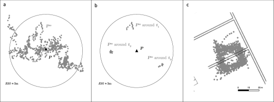
Figure 4: The distribution of GPS measurement error at position $\boldsymbol{P}$ (a). Revealing the temporal autocorrelation of GPS measurement error (b). The movement of a pedestrian around a reference course (c).

5.1 Experiment 1: Pedestrian trajectories

Experimental setup

For the first experiment, we equipped a pedestrian with a GPS. The pedestrian walked along a reference course with a well-established reference distances $d_{0}$. The movement of the pedestrian was recorded with a QSTARZ:BT-Q1000X GPS unit with ‘Assisted GPS’ activated.

Rather than using a high-quality GPS we collected all data with a low-budget GPS, a type of GPS common for recording movement data. We deliberately treated the GPS as a ‘black box’. This implies that the algorithm to calculate the position estimates from the raw GPS signal was not known. Moreover, we considered that it was sufficient to use only a single GPS unit, as the aim of the experiment was not to investigate the quality of the particular GPS, but to show the usefulness of our approach.

The reference course was located in an empty parking lot to avoid shadowing and multi-path effects. We staked out a square with sides that were $10~{}\mathrm{m}$ long and had markers at one meter intervals. A square was used in order to allow distance measurements to be collected in all four cardinal directions (approximately). The distance between the markers was used as a reference distance $d_{0}$.

The GPS position estimates were obtained by walking to the reference markers in turn and recording the position, moving around the square until all positions of the markers had been recorded. Position estimates were only taken at the reference markers, and only when the recording button was pushed manually. Two consecutive position estimates were taken within three to five seconds. A full circuit around the square took approximately between two and three minutes and resulted in $40$ positions being recorded. A total of $25$ circuits around the square were completed, without any breaks. This resulted in $1000$ GPS positions being collected in approximately one hour.

In pre-processing distance measurements $d^{m}$ were calculated between the position estimates and later compared to $d_{0}$ the reference distance between the markers. Then the average measured distance $\bar{d^{m}}$ was calculated and from this $\hat{\mathit{OD}}=\bar{d^{m}}-d_{0}$ and $\hat{C}=d^{2}_{0}-\bar{d^{m}_{2}}+\textit{Var}_{\textit{gps}}$ were derived. $\mathit{\hat{OD}}$ and $\hat{C}$ are estimators for $\mathit{OD}$ and $C$.

We decided not to derive $\sigma_{X}$ and $\sigma_{Y}$ from observational data, but to set $\sigma_{X}=\sigma_{Y}=3\mathrm{m}$. Hence, $\textit{Var}_{\textit{gps}}$ is not the observed variance of GPS measurement error, but a reference value to which $\mathit{OD}$ is later compared to. Consequently, our results do not show the exact value of $C$, but provide an estimate of $C$ with respect to $\textit{Var}_{\textit{gps}}$.

We increased the spatial separation between two position estimates of the pedestrian to illustrate the influence of spatial autocorrelation. Then we increased the temporal separation between two position estimates to illustrate the influence of temporal autocorrelation.

Results

In contrast to the theoretical findings in Figure 3, overestimation of distance tended to increase as the reference distance $d_{0}$ increased. This was due to a decrease in the spatial autocorrelation of GPS measurement error. With increasing spatial separation of the position estimates, measurement error became less auto-correlated. Figure 5 shows the relationship between the reference distance $d_{0}$ and $\hat{\mathit{OD}}$ (black dots) as well as $\hat{C}$ (black crosses).

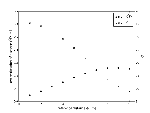
Figure 5: Overestimation of distance ($\hat{\mathit{OD}}$) and spatial autocorrelation of GPS measurement error ($\hat{C}$) in the pedestrian movement data.

We wanted to illustrate that the overestimation of distance was not caused by a small number of extreme outliers. Figure 6 shows the histogram of $d^{m}-d_{0}$ for $d_{0}=1~{}\mathrm{m}$ (a), and for $d_{0}=5~{}\mathrm{m}$ (b) and their fit to a Gaussian distribution. Both histograms follow a Gaussian distribution $\mathcal{N}(\mu_{d},\sigma^{2}_{d})$ rather well and outliers are almost non-existent. Note that $\mu_{d}$ and $\sigma^{2}_{d}$ in Figure 6 refer to the values of the fitted Gaussian distribution and not to the empirically derived frequency.

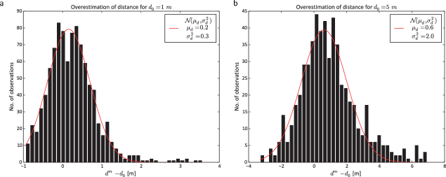
Figure 6: Histogram of the difference between measured and reference distance ($d^{m}-d_{0}$) for $d_{0}=1~{}\mathrm{m}$ (a) and $d_{0}=5~{}\mathrm{m}$ (b)

In order to illustrate the temporal autocorrelation in GPS measurement error, we calculated the distance between non-consecutive position estimates around the square. One example is the distance between two position estimates, where the second one was obtained one circuit after the first later. The reference distance between the markers remained the same, e.g. $d_{0}=1~{}\mathrm{m}$, but the position estimates were recorded within a longer time interval $\Delta t$. Figure 7 shows the relationship between $\Delta t$ and $\hat{\mathit{OD}}$ (black dots) as well as $\hat{C}$ (black crosses) for a reference distance $d_{0}=1~{}\mathrm{m}$. $\hat{\mathit{OD}}$ increase with longer time intervals. The sharpest increase occurs between measurements that were taken promptly and those taken after about $2{\frac{1}{2}}$ minutes. After $40$ minutes the curve levels out. This increase of $\hat{\mathit{OD}}$ was caused by the temporal auto-correlation of measurement error. For measurements taken within several seconds, measurement error appears to be strongly auto-correlated. However, auto-correlation falls sharply for measurements taken within $2{\frac{1}{2}}$ minutes. From then on $\hat{C}$ gradually decreases as $\Delta t$ increases; again the curve levels out at about $40$ minutes.

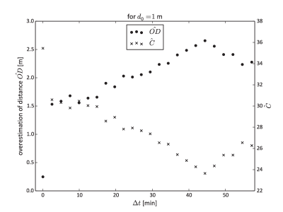
Figure 7: Overestimation of distance $\hat{\mathit{OD}}$ and temporal autocorrelation of GPS measurement error ($\hat{C}$) in the pedestrian movement data.

The data for the above experiment were calculated with a GPS for which the algorithm to calculate the position estimates from the raw GPS signal was not known. This raises the legitimate question, whether the results were produced by a smoothing algorithm rather than the behaviour of the GPS. Let us assume that the GPS used a smoothing algorithm. In simplified form, the current position estimate is then calculated from the last position estimate, the current GPS measurement and a movement model. For movement with constant speed and direction, smoothing yields trajectories that represent the true movement very accurately. However, sudden changes in movement, i.e. a sharp turn, are not followed by the trajectory. The current measurement implies a sharp turn, however, the movement model does not. Thus, the sharp turn becomes more elongated, the overestimation of distance increases. However, we did not find any support for an increase in the overestimation of distance after a sharp turn. This can also be seen in Figure 4 b.

5.2 Experiment 2: Car trajectories

In the first experiment the reference distance $d_{0}$ was staked out along a reference course. For obvious reasons this is not possible for recording the movement of a car. Hence we derived $d_{0}$ from speed measurements recorded with a car’s controller area network bus (CAN bus).

Experimental Setup

We equipped a car with a GPS unit and tracked its movement for about 6 days. The car moved mostly in an urban road network at rather low speeds (average: $25~{}\mathrm{km/h}$). The temporal sampling rate of recording was $1~{}\mathrm{Hz}$. For the CAN bus measurements, a sensor recorded the rotation of the car’s drive axle, from which $d_{0}$ was inferred. Thus $d_{0}$ is the distance travelled by the car according to the CAN bus. For the same phases of movement we compared $d_{0}$ to $d^{m}$, the distance travelled by the car according to the GPS position estimates. As in the first experiment, we set $\sigma_{X}=\sigma_{Y}=3\mathrm{m}$ and calculated $\textit{Var}_{\textit{gps}}$.

The data were first pre-processed and cleaned. Parts with very high speed (above $140~{}\mathrm{km/h}$) and very rapid acceleration (above $5~{}\mathrm{m/s^{2}}$) were removed. Although the data consisted mostly of the car’s forward movements, there were also periods when it was either stationary or reversing in a parking lot. The data may also have included some periods during which shadowing caused a loss of the GPS signal (for example when driving in a tunnel). We therefore applied a simple mode detection algorithm to remove any such periods. The algorithm evaluates speed and acceleration along the trajectory and distinguishes segments that most probably reflect driving behaviour from those that are likely to reflect non-driving behaviour (Zheng et al., 2010). Using the algorithm we were able to include only long phases of continuous driving, sampled at a continuous sampling frequency of $1~{}\rm{Hz}$. Following this pre-processing a total of about $195~{}\mathrm{km}$ of car trajectories remained for analysis.

Results

Figure 8 shows that the autocorrelation of GPS measurement error decreased as the spatial separation between two consecutive position estimates increased. Nevertheless, $\hat{C}$ in Figure 8 is always positive. This can be interpreted as a quality measure for the movement data. Consecutive position estimates were affected by less variance than initially suggested by $\textit{Var}_{\textit{gps}}$.

Although the results in Figure 8 are similar to those obtained from the pedestrian movement data, they contain outliers. We believe that these outliers occur due to two reasons. First, the data comprise relatively few distance measurements for big $d_{0}$ because of the generally low speed of the car. Second, we could not guarantee a full temporal synchronization of both measurement systems (GPS and CAN bus). In other words, $d_{0}$ and $d^{m}$ might relate to slightly different time intervals. We found this lag to be around one second. We believe that this insight is important for the practical application of Equation 7. In order to provide valid results it requires both a significant number of distance measurements as well as a proper synchronisation of reference and measured distance.

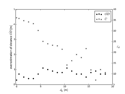
Figure 8: Overestimation of distance ($\hat{\mathit{OD}}$) and spatial autocorrelation of GPS measurement error ($\hat{C}$) in the car movement data.

6 Discussion and Outlook

In this paper we identified a systematic bias in GPS movement data. If interpolation error can be neglected GPS trajectories systematically overestimate distances travelled by a moving object. This overestimation of distance has previously been noted in the trajectories of fishing vessels (Palmer, 2008). For high sampling rates the distance travelled by the vessel was overestimated due to measurement error, while for lower sampling rates it was underestimated due to the influence of interpolation error. We provided a mathematical explanation for this phenomenon and showed that it functionally depends on three parameters, of which one is $C$, the spatio-temporal autocorrelation of GPS measurement error. We built on this relationship and introduced a novel approach to estimate $C$ in real-world GPS movement data. In this Section we want to discuss our findings and show their implications for movement analysis and beyond.

In the era of big data, more and more movement data are recorded at finer and finer intervals. For movement recorded at very high frequencies (e.g. $1\rm{Hz}$) interpolation error can usually be neglected. Hence $\mathit{OD}$ is bound to occur in these data. However, this does not mean that high frequency movement data are of low quality, quite the opposite is true. Using the relationship between $C$ and $\mathit{OD}$ we showed experimentally that GPS measurement error in real world trajectories was affected by strong spatial and temporal autocorrelation. In other words, if the data were recorded close in space and time they captured the movement of the object better than if they were further apart.

Autocorrelation is important for movement analysis in many aspects. An appropriate sampling strategy for recording movement data, for example, should consider the influence of measurement error and address spatial and temporal autocorrelation. Since autocorrelation can be interpreted as a quality measure, it allows to reveal the performance of different GPS receivers in different recording environments. Moreover, autocorrelation has implications for simulation. Laube and Purves (2011) performed a simulation to reveal the complex interaction between measurement error and interpolation error and their effects on recording speed, turning angle and sinuosity. Their Monte Carlo simulation assumed GPS errors to scatter entirely randomly between each two consecutive positions. Our approach allows to verify whether this assumption is realistic.

Where to find a reference distance?

For practical applications the biggest limitation of our experiments is their dependency on a valid reference distance. The moving object must traverse the reference distance along a straight line and without interpolation error, and at a precisely known time. Moreover, a large number of measurements has to be collected, since $C$ is derived from the expectation value of a random variable.

This limitation leads to a possibly interesting application of our findings, where the reference distance is derived from the GPS point speed measurements. Point speed measurements are calculated from the instantaneous derivative of the GPS signal using the Doppler effect. Point speed is very accurate (Bruton et al., 1999) and usually part of a GPS position estimate. Hence, for high sampling rates (e.g.$1$ Hz) point speed measurements can be used to infer the distance that a moving object has travelled between two position estimates. This distance is not affected by the overestimation of distance effect and could serve as a reference distance. Thus, GPS could be compared to itself to reveal the spatio-temporal autocorrelation of the position estimates. This approach would not require any other ground truth data. However, its feasibility and usefulness are yet to be tested.

Finally, we want to underline that our findings are not only relevant for GPS. The overestimation of distance is bound to occur in any type of movement data where distances are deduced from imprecise position estimates, of course only if interpolation error can be neglected.

References

- Andrienko et al. (2011) Andrienko, G., Andrienko, N., and Heurich, M., 2011. An event-based conceptual model for context-aware movement analysis. International Journal of Geographical Information Science, 25 (9), 1347–1370.
- Bos et al. (2008) Bos, M., et al., 2008. Fast error analysis of continuous GPS observations. Journal of Geodesy, 82 (3), 157–166.
- Bruton et al. (1999) Bruton, A., Glennie, C., and Schwarz, K., 1999. Differentiation for high-precision GPS velocity and acceleration determination. GPS solutions, 2 (4), 7–21.
- Chin (1987) Chin, G.Y., 1987. Two-dimensional Measures of Accuracy in Navigational Systems. Report DOT-TSC-RSPA-87-1, U.S. Department of Transportation.
- Codling et al. (2008) Codling, E.A., Plank, M.J., and Benhamou, S., 2008. Random walk models in biology. Journal of the Royal Society Interface, 5 (25), 813–834.
- Colombo (1986) Colombo, O.L., 1986. Ephemeris errors of GPS satellites. Bulletin géodésique, 60 (1), 64–84.
- D’Eon et al. (2002) D’Eon, R.G., et al., 2002. GPS radiotelemetry error and bias in mountainous terrain. Wildlife Society Bulletin, 430–439.
- Douglas-Hamilton et al. (2005) Douglas-Hamilton, I., Krink, T., and Vollrath, F., 2005. Movements and corridors of African elephants in relation to protected areas. Naturwissenschaften, 92 (4), 158–163.
- El-Rabbany and Kleusberg (2003) El-Rabbany, A. and Kleusberg, A., 2003. Effect of temporal physical correlation on accuracy estimation in GPS relative positioning. Journal of Surveying Engineering, 129 (1), 28–32.
- Güting and Schneider (2005) Güting, R. and Schneider, M., 2005. Moving objects databases. San Francisco: Morgan Kaufmann.
- Higuchi and Pierre (2005) Higuchi, H. and Pierre, J.P., 2005. Satellite tracking and avian conservation in Asia. Landscape and Ecological Engineering, 1 (1), 33–42.
- Hofmann-Wellenhof et al. (2003) Hofmann-Wellenhof, B., Legat, K., and Wieser, M., 2003. Navigation: Principles of positioning and guidance. Wien: Springer Verlag.
- Howind et al. (1999) Howind, J., Kutterer, H., and Heck, B., 1999. Impact of temporal correlations on GPS-derived relative point positions. Journal of Geodesy, 73 (5), 246–258.
- Jerde and Visscher (2005) Jerde, C.L. and Visscher, D.R., 2005. GPS measurement error influences on movement model parameterization. Ecological Applications, 15 (3), 806–810.
- Jun et al. (2006) Jun, J., Guensler, R., and Ogle, J.H., 2006. Smoothing methods to minimize impact of Global Positioning System random error on travel distance, speed, and acceleration profile estimates. Transportation Research Record: Journal of the Transportation Research Board, 1972 (1), 141–150.
- Klenke (2013) Klenke, A., 2013. Probability theory: a comprehensive course. Springer Science & Business Media.
- Langley (1997) Langley, R.B., 1997. The GPS error budget. GPS world, 8 (3), 51–56.
- Laube and Purves (2011) Laube, P. and Purves, R.S., 2011. How fast is a cow? Cross-Scale Analysis of Movement Data. Transactions in GIS, 15 (3), 401–418.
- Macedo et al. (2008) Macedo, J., et al., 2008. 5. In: Trajectory Data Models., 123 – 150 Berlin: Springer.
- Mintsis et al. (2004) Mintsis, G., et al., 2004. Applications of GPS technology in the land transportation system. European Journal of Operational Research, 152 (2), 399–409.
- Modsching et al. (2006) Modsching, M., Kramer, R., and ten Hagen, K., 2006. Field trial on GPS Accuracy in a medium size city: The influence of built-up. In: 3rd Workshop on Positioning, Navigation and Communication, 209–218.
- Olynik (2002) Olynik, M., 2002. Temporal characteristics of GPS error sources and their impact on relative positioning. Report, University of Calgary.
- Palmer (2008) Palmer, M.C., 2008. Calculation of distance traveled by fishing vessels using GPS positional data: A theoretical evaluation of the sources of error. Fisheries Research, 89 (1), 57–64.
- Parent et al. (2013) Parent, C., et al., 2013. Semantic trajectories modeling and analysis. ACM Computing Surveys, 45 (4), 1–32.
- Schneider (1999) Schneider, M., 1999. In: Uncertainty management for spatial data in databases: Fuzzy spatial data types., 330–351 Berlin: Springer.
- Sigrist et al. (1999) Sigrist, P., Coppin, P., and Hermy, M., 1999. Impact of forest canopy on quality and accuracy of GPS measurements. International Journal of Remote Sensing, 20 (18), 3595–3610.
- Van der Spek et al. (2009) Van der Spek, S., et al., 2009. Sensing human activity: GPS tracking. Sensors, 9 (4), 3033–3055.
- Wang et al. (2002) Wang, J., Satirapod, C., and Rizos, C., 2002. Stochastic assessment of GPS carrier phase measurements for precise static relative positioning. Journal of Geodesy, 76 (2), 95–104.
- Wang et al. (2014) Wang, J., et al., 2014. A novel approach for generating routable road maps from vehicle GPS traces. International Journal of Geographical Information Science, 29 (1), 69–91.
- William J. Hughes Technical Center (2013) William J. Hughes Technical Center, 2013. Global Positioning System (GPS) Standard Positioning Service (SPS) Performance Analysis Report . Report, Federal Aviation Administration.
- Wing et al. (2005) Wing, M.G., Eklund, A., and Kellogg, L.D., 2005. Consumer-grade global positioning system (GPS) accuracy and reliability. Journal of Forestry, 103 (4), 169–173.
- Zandbergen (2009) Zandbergen, P.A., 2009. Accuracy of iPhone locations: A comparison of assisted GPS, WiFi and cellular positioning. Transactions in GIS, 13 (s1), 5–25.
- Zheng et al. (2010) Zheng, Y., et al., 2010. Understanding transportation modes based on GPS data for web applications. ACM Transactions on the Web (TWEB), 4 (1), 1.
- Zheng et al. (2011) Zheng, Y., et al., 2011. Urban computing with taxicabs. In: Proceedings of the 13th international conference on Ubiquitous computing, 89–98.
- Zito et al. (1995) Zito, R., d’Este, G., and Taylor, M.A., 1995. Global positioning systems in the time domain: How useful a tool for intelligent vehicle-highway systems?. Transportation Research Part C: Emerging Technologies, 3 (4), 193–209.