Spatial Product Partition Models

Abstract

When modeling geostatistical or areal data, spatial structure is commonly accommodated via a covariance function for the former and a neighborhood structure for the latter. In both cases the resulting spatial structure is a consequence of implicit spatial grouping in that observations near in space are assumed to behave similarly. It would be desirable to develop spatial methods that explicitly model the partitioning of spatial locations providing more control over resulting spatial structures and being able to better balance global vs local spatial dependence. To this end, we extend product partition models to a spatial setting so that the partitioning of locations into spatially dependent clusters is explicitly modeled. We explore the spatial structures that result from employing a spatial product partition model and demonstrate its flexibility in accommodating many types of spatial dependencies. We illustrate the method’s utility through simulation studies and an education application. Computational techniques with additional simulations and examples are provided in a Supplementary Material file available online.

Key Words: prediction; product partition models, spatial smoothing, spatial clustering.

1 Introduction

Research dedicated to developing statistical methodologies that in some way incorporate information relating to location has grown exponentially in the last decade. In fact, spatial methods are now available in essentially all areas of statistics and have been developed to accommodate both areal (lattice) and geo-referenced data. The principal motivation in developing these methods is to produce inference and predictions that take into account the spatial dependence that is believed to exist among observations. The end result is typically a smoothed map for areal data or a predictive map for geo-referenced data. These maps are frequently produced by implicitly performing a type of spatial grouping that carries out the intuitively appealing notion that responses measured at locations near in space have similar values. Since the grouping is implicit, the spatial partition is not directly modeled but is a consequence of model choices (e.g., neighborhood structure or covariance function). For areal data this can lead to spatial correlation structures that are counter-intuitive (Wall:2004). Additionally, it is common that the smoothed or predictive maps are global in nature in that methods are not flexible enough to capture local deviations from an overall spatial structure.

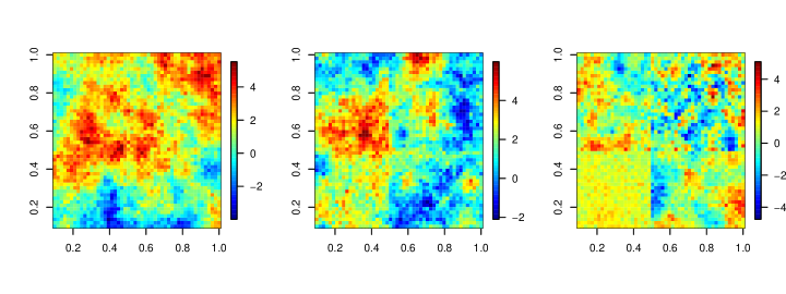
Figure 1: Synthetic spatial fields. From left to right, the graphs display random fields that become progressively more local.

Figure 1 provides a synthetic example of local vs. global spatial dependence. The three plots were generated using a Gaussian process featuring an exponential covariance function. From left to right the random fields become increasingly more local. The left plot displays one spatial process over the entire domain that has expectation 0, nugget 0.1, partial sill 2, and effective range 6 (see GelfandBook for more details). The second plot is generated with the same covariance function, but the field is partitioned into four rectangular clusters and each is assigned a specific constant mean $(1,-0.5,0.25,-1)$, thus inducing a small amount of local structure. The right plot is the most local of the three as each cluster is a realization from a unique spatial process that has expectation 0 and a cluster specific partial sill $(1,2,3,4)$ and effective range $(0.5,10,5,20)$. Methods able to flexibly capture these three structures would certainly be appealing. Developing these types of methods is the primary focus of this paper.

Our approach is to develop a class of priors based on product partition models (PPM, PartitionModels) that directly model the partitioning of locations into spatially dependent clusters. Making the PPM location dependent is necessary in a spatial setting because if not, then locations that are very far apart could possibly be assigned to the same cluster with high probability. As a consequence, the marginal correlation between observations far apart could be stronger than that of observations near each other, which runs counter to correlation structures often desired in spatial modeling. As will be seen, PPM’s are a very attractive way to partition spatial units as they are extremely flexible in accommodating different types of spatial clusters.

The method we develop is able to adapt to the three scenarios described in Figure 1 by incorporating spatial information in two ways. The first is via a prior on the partitioning of locations using PPM ideas. The second is through the likelihood either directly or hierarchically. If spatial structure is not built in the likelihood, the spatial PPM will marginally induce local spatial dependence among observations. As an aside, apart from more accurately modeling spatial phenomena, considering local spatial dependance potentially provides large computational gains as covariance matrices are considerably smaller.

Spatial methods now have a large presence in the statistical literature. We focus on methods that incorporate spatial dependence flexibly. For a general overview of spatial methods see gelfand2010handbook, GelfandBook, or GotwayBook.

Locating spatial clusters is commonly considered in spatial point processes (DiggleBook). That said, from a modeling standpoint, the analysis goals are completely different from those we consider. Image segmentation is an extensively studied area that we do not attempt to fully survey here. We do mention the spatial distance dependent Chinese restaurant process of NIPS2011_0843 (a spatial extension of the distance dependent Chinese restaurant process of ddCRP) as they develop a process that produces a non-exchangeable distribution on location dependent partitions through a distance dependent decay function. Though there are similarities, our approach is model based and therefore provides measures of uncertainty regarding inferences and predictions.

sDP developed a spatial Dirichlet process (DP) by modeling atoms associated with Sethuraman:1994’s stick-breaking random measure construction with a random field. gsDP generalized the spatial DP through a type of multivariate stick-breaking in which individual sites could possibly arise from unique surfaces introducing a type of local spatial modeling. Both spatial DP processes require replication. obDDP developed the ordered dependent DP where stick breaking weights are randomly permuted according to a latent spatial point process thus inducing spatial dependence. hDP developed a DP that pieces together functions and applied it to a spatial field. spatialDPclustering use a DP to model locations directly resulting in spatially referenced clusters. All of these methods induce a marginal distribution on partitions through the introduction of latent cluster labels.

Somewhat related to the spatial DP and operationally similar to what we introduce are the spatial stick-breaking process of SSB and the logistic stick-breaking process of logisticSB (both of which are in some sense special cases of kernel-stick breaking process of KSB). Both stick-breaking processes induce spatial dependence via kernel functions that allow stick-breaking weights to change with space. A related probit-stick breaking prior for spatial dependence was recently proposed in papageorgiouetal:14.

Other authors have employed DP type methods to areal data resulting in a more flexible (local) neighborhood structure (Hanson:2014, BayesianLocalConditionalAutoregressiveModel). Kang:2014 created local conditional autoregressive (CAR) models to accommodate local spatial residual.

Even though all the previously mentioned nonparametric Bayes based methods may have some inferential similarities or are at least operationally similar to what we are proposing, they are fundamentally different. We do not introduce any notion of a random probability measure. Therefore, we are not bound to an induced marginal model on partitions available from the DP (though this particular model is certainly available as a special case). Instead we directly model the spatially dependent partition using a PPM. Doing so provides much more control over the partitioning of spatial units into clusters.

From a disease mapping perspective, BayesianPartitioningforEstimatingDiseaseRisk consider spatial clustering by first selecting cluster centroids and using tessellation ideas of SpatialClusterModeling to determine cluster memberships. This requires employing Reversible Jump MCMC and produces spatial clusters that are necessarily convex. BayesianDetectionofClustersandDiscontinuitiesinDiseaseMaps cluster areal units via a distance measure that is based on shared boundaries. BayesianDiseaseMappingUsingProductPartitionModels employ a PPM to model partitions of areal units, though they do not explore the spatial properties of their model and are restricted to a very specific setting. We aim to propose a very general methodology that is flexible in accommodating many types of spatial dependencies. In fact, we will show that once a model for the partition has been specified, the sky is limit in terms of how spatial dependence can be incorporated in other parts of the model.

The remainder of the article is organized as follows. In Section 2 we provide some preliminaries on PPM’s and a bit of discussion on spatial clustering. Section 3 details spatial extensions of the PPM and investigates spatial properties. Section 4 contains a small simulation study and a Chilean education data application. We make some concluding remarks in Section 5. Lastly, the Supplementary Material file available online contains computational details along with additional simulations and applications.

2 Preliminaries

We provide background to PPM’s and a bit of discussion motivating our view of spatial clusters.

2.1 Preliminaries of Product Partition Model

PPM’s were first introduced by PartitionModels and have since been extended to include covariates (PPMxMullerQuintanaRosner and bgPPM) and correlated parameters (PPMcorrelatedParameters). They’ve been employed in applications ranging from change point analysis (PPMchangePoint) to functional clustering (Page:2014) among others. Since PPMs are central to our approach of carrying out spatial clustering, we briefly introduce them here. Consider $n$ distinct locations denoted by $\bm{s}_{1},\ldots,\bm{s}_{n}$. The $\bm{s}_{i}$ are quite general in that they can be latitude and longitude values or in the case of areal data they could define a neighborhood structure. The goal is to directly model the partitioning of the $\bm{s}_{i}$, $i=1,\ldots,n$ into $k_{n}$ groups. With this in mind, let $\rho_{n}=\{S_{1},\ldots,S_{k_{n}}\}$ denote a partitioning (or clustering) of the $n$ locations into $k_{n}$ subsets such that $i\in S_{h}$ implies that location $i$ belongs to cluster $h$. Alternatively, we will denote cluster membership using $c_{1},\ldots,c_{n}$ where $c_{i}=h$ implies $i\in S_{h}$. Then the PPM prior for $\rho$ is simply

$$Pr(\rho)\propto\prod_{h=1}^{k_{n}}C(S_{h}),$$ (2.1)

where $C(S_{h})\geq 0$ for $S_{h}\subset\{1,\ldots,n\}$ is a cohesion function that measures how likely elements of $S_{h}$ are clustered a priori. The normalizing constant of (2.1) is simply the sum of (2.1) over all possible partitions. A popular cohesion function that connects (2.1) to the marginal prior distribution on partitions induced by a Dirichlet process (DP) is $C(S)=M\times\Gamma(|S|)$. This cohesion produces a PPM that encourages partitions with a small number of large clusters and also a few smaller clusters (the rich get richer property). This property will be useful to avoid creating many singleton clusters when extending PPM’s to a spatial setting and therefore the form $M\times\Gamma(|S|)$ will be used regularly. Eventually we will consider a response and covariate vector measured at each location which will be denoted by $y(\bm{s}_{i})$ and $\bm{x}(\bm{s}_{i})$ respectively. Finally, it will be necessary to make reference to partitioned location and response vectors which we denote by $\bm{s}^{\star}_{h}=\{\bm{s}_{i}:i\in S_{h}\}$ and $\bm{y}_{h}^{\star}=\{y(\bm{s}_{i}):i\in S_{h}\}$.

2.2 Spatial Clustering

Before proceeding, we expound on the term “spatial cluster” and make its definition used in this paper concrete (for more discussion on the subject of spatial clusters see BayesianDiseaseMapping). Typically, clustering attempts to group or partition individuals or experimental units based on some measured response variable. Therefore, the resulting partition consists of clusters whose members are fairly homogenous with respect to the measured response. How cluster boundaries are defined (e.g., elliptical, convex) is crucial to the resulting partition and to our knowledge no universally agreed upon definition exists. When in addition to a measured response, the proximity of individuals or experimental units influences the partitioning of individuals, then we refer to these clusters as “spatial”.

If spatial structure exists among the realizations of some response variable measured at various locations, then the values measured at locations near each other should be more similar than those that are far apart. However, this doesn’t exclude the possibility of two individuals far apart producing similar responses. Clustering in the absence of spatial information would group these two individuals together (as would be the case in a non-spatial PPM). From a spatial perspective it seems more natural that locations far from each other would not belong to the same cluster. That is, spatial clusters should be in some sense “local” in that locations that belong to the same cluster should share a boundary for areal data (or comply with some other neighborhood structure) or attain a pre-determined minimum distance with other members of the cluster for geo-referenced data. We make this concrete with the following definition.

Definition 2.1.

Consider $\bm{s}^{\star}_{h}$ corresponding to cluster $S_{h}\subset\{1,\ldots,n\}$ and let $d(\cdot,\cdot)$ be a metric in the space of spatial coordinates. We say that cluster $S_{h}$ is spatially connected if there does not exist $\bm{s}_{i^{\prime}}\notin\bm{s}^{\star}_{h}$ such that for all $\bm{s}_{i},\bm{s}_{j}\in\bm{s}^{\star}_{h}$ where $\bm{s}_{j}\neq\bm{s}_{i}$, $d(\bm{s}_{i^{\prime}},\bm{s}_{i})<d(\bm{s}_{j},\bm{s}_{i})$. A partition will be called spatially connected if all of its clusters are spatially connected.

Figure 2 provides four spatial plots of regular grids that assist in visualizing spatially connected clusters. The top left plot is an example of convex clusters that are connected while the top right plot contains connected clusters one of which is concave. The bottom left plot is an example of a partition that is not connected as the cluster of triangle points has been split by the cluster of square points. The bottom right plot is an example of clusters that are connected even though there exists a singleton island cluster.

Figure 2: Regular grids that provide an illustration of spatial connectedness. The top two figures display partitions that are spatially connected with the left demonstrating concave clusters and the right convex. The bottom left graph illustrates a partition that is not spatially connected as the green cluster is not spatially connected since it has been completely separated by the red. The partition in the bottom right figure is spatially connected even though there exists an island (singleton) cluster.

Our vision of spatial clusters does not necessarily partition the spatial domain into disjoint sets. Because clusters possibly depend on variables other than location, it is possible that two clusters exist in the same geographical region. The presence of these “stacked” clusters seems common and a perk of the methodology we develop.

3 Methodological Development

We now detail spatial extensions to the basic PPM (here after referred to as sPPM) and investigate cluster membership probabilities. Also, we show that combining sPPM with likelihoods (that potentially include spatial information) produce marginal spatial structures with appealing properties (e.g., non-stationary) and balance local vs. global structure. As both cluster membership probabilities and correlations depend on the cohesion function we propose a few reasonable candidates.

3.1 Cohesion Functions

Extending the PPM to incorporate spatial information requires making the cohesion of (2.1) a function of location. With this in mind, consider

$$Pr(\rho)\propto\prod_{h=1}^{k_{n}}C(S_{h},\bm{s}^{\star}_{h}),$$ (3.1)

which makes the clustering process location dependent. (This is structurally similar to bgPPM’s approach to extending the PPM to incorporate covariates.) Defining a cohesion function that only admits spatially connected partitions is conceptually straightforward. For example, one could employ

$$C(S,\bm{s}^{\star}_{h})=\left\{\begin{array}[]{l l}M\times\Gamma(|S|)&\quad\mbox{if $S$ is spatially connected }\\ 0&\quad\text{otherwise,}\end{array}\right.$$

where $M\times\Gamma(|S|)$ is used to favor a small number of large clusters with the number of clusters being regulated by $M$. A cohesion function defined in this way places zero prior mass on partitions that are not spatially connected. Although this definition is intuitively appealing, it is particularly challenging to implement from a computational stand point and can only realistically be considered for a small number of locations. Therefore, we suggest considering cohesion functions that assign small probabilities to partitions with clusters that are not spatially connected. A nice feature of the sPPM is that there are many ways in which this can be carried out and we introduce four reasonable candidates. Subsequently, we study the spatial properties of each one.

As we introduce the first cohesion function keep in mind that our overarching goal is to develop a prior that favors spatially connected partitions without creating a bunch of singleton clusters. One way to carry this out is by employing tessellation ideas found in BayesianPartitioningforEstimatingDiseaseRisk in that distances to a cluster centroid are considered. To this end, let $\bar{\bm{s}}_{h}$ denote the centroid of cluster $S_{h}$ and $\mathcal{D}_{h}=\sum_{i\in S_{h}}d(\bm{s}_{i},\bar{\bm{s}}_{h})$ the sum of all distances from the centroid (unless otherwise stated we use Euclidean norm $\|\cdot\|$). Defining the cohesion as a decreasing function of $\mathcal{D}_{h}$ would certainly produce small local clusters. Unfortunately, cohesions that favor clusters with small $\mathcal{D}_{h}$ would also produce partitions with many singleton clusters. To counteract this, we make the cohesion a function of $M\times\Gamma(|S_{h}|)$ in addition to $\mathcal{D}_{h}$. Now since $\Gamma(|S_{h}|)$ would overwhelm $\mathcal{D}_{h}$ as cluster membership grows, we consider $\Gamma(\mathcal{D}_{h})\mathbb{I}[\mathcal{D}_{h}\geq 1]+\mathcal{D}_{h}\mathbb{I}[\mathcal{D}_{h}<1]$. (The partitioning of $\mathcal{D}_{h}$’s domain was motivated by the fact that the gamma function is not monotone on $[0,1]$ and does not tend to zero as $\mathcal{D}_{h}$ tends to zero). Finally, to provide a bit more control over the penalization of distances, we introduce a user supplied tuning parameter, $\alpha$, resulting in the following cohesion function

$$C_{1}(S_{h},\bm{s}^{\star}_{h}) =\left\{\begin{array}[]{cc}\dfrac{M\times\Gamma(|S_{h}|)}{\Gamma(\alpha\mathcal{D}_{h})\mathbb{I}[\mathcal{D}_{h}\geq 1]+(\mathcal{D}_{h})\mathbb{I}[\mathcal{D}_{h}<1]}&\mbox{if $|S_{h}|>1$}\\ \\[-14.22636pt] M&\mbox{if $|S_{h}|=1$}.\end{array}\right.$$ (3.5)

We set $C_{1}(S_{h},\bm{s}^{\star}_{h})=M$ for $|S_{h}|=1$ to avoid issues associated with $\mathcal{D}_{h}=0$. Notice that since all $\bm{s}_{1},\ldots,\bm{s}_{n}$ are distinct $\mathcal{D}_{h}=0\iff|S_{h}|=1$. Further, when $|S_{h}|=1$, $M\times\Gamma(|S_{h}|)=M$ justifying in a sense setting the cohesion to $M$ when $|S_{h}|=1$.

The second cohesion function we consider provides a hard cluster boundary and for some pre-specified $a>0$ has the following form

$$C_{2}(S_{h},\bm{s}^{\star}_{h}) =M\times\Gamma(|S_{h}|)\times\prod_{i,j\in S_{h}}\mathbb{I}[\lVert\bm{s}_{i}-\bm{s}_{j}\rVert\leq a].$$ (3.6)

Once again, $M\times\Gamma(|S_{h}|)$ is included to inherit the “rich get richer” property of DP partitioning. This cohesion is amenable to neighborhood structures of areal data modeling. Instead of $\mathbb{I}[d(\bm{s}_{i},\bm{s}_{j})\leq a]$, one could use $\mathbb{I}[i\sim j]$ where $i\sim j$ indicates that $\bm{s}_{i}$ and $\bm{s}_{j}$ are neighbors according to some neighborhood structure. If a data dependent neighborhood structure is desired, one could introduce auxiliary variables in the cohesion and employ ideas similar to those found in Kang:2014.

sPPM under $C_{1}$ and $C_{2}$ produces a completely valid joint distribution over partitions that is quite general. In fact, since the cohesions are functions of not only $|S_{h}|$ but also of $\bm{s}^{\star}_{h}$, sPPM relaxes exchangeability assumptions. However, for this same reason sPPM under $C_{1}$ and $C_{2}$ does not inherit the PPM (2.1)’s property of being coherent across sample sizes. That is, $P(\rho_{n})\neq\sum_{h=1}^{k_{n}+1}P(\rho_{n},c_{n+1}=h)$. This is easily seen as the location of $s_{n+1}$ influences $P(\rho_{n},c_{n+1}=j)$. Although this does not change the fact that the sPPM produces a valid joint distribution over partitions, for computational purposes it is sometimes desirable to have coherence across sample sizes. To retain this property one would need to “marginalize” over all possible locations. This was considered in detail in PPMxMullerQuintanaRosner (and also mentioned in bgPPM) when making a PPM covariate dependent. We employ ideas developed in PPMxMullerQuintanaRosner in a spatial setting which produces the following cohesion

$$C_{3}(S_{h},\bm{s}^{\star}_{h}) =M\times\Gamma(|S_{h}|)\times\int\prod_{i\in S_{h}}q(\bm{s}_{i}|\bm{\xi}_{h})q(\bm{\xi}_{h})d\bm{\xi}_{h}.$$ (3.7)

In Bayesian modeling $\int\prod_{i\in S_{h}}q(\bm{s}_{i}|\bm{\xi}_{h})q(\bm{\xi}_{h})d\bm{\xi}_{h}$ is often called the marginal likelihood or prior predictive distribution and is used to measure the similarity among the locations belonging to cluster $h$. Therefore, $C_{3}$ favors partitioned location vectors ($\bm{s}^{\star}$) that produce large marginal likelihood values. To simplify evaluating $C_{3}$ and retain coherence across sample sizes, $q(\bm{s}|\bm{\xi})$ and $q(\bm{\xi})$ are specified to form a conjugate probability model. We emphasize however that we are not assuming the $\bm{s}_{i}$’s to be random, we are simply employing the conjugate model as a means to measure spatial proximity and encourage co-clustering of locations that are near each other. Both areal and point referenced data can be considered when $C_{3}$ is employed, all that is required is specifying appropriate $q(\bm{s}|\bm{\xi})$ and $q(\bm{\xi})$. For example, if point referenced data are available, a conjugate Gaussian/Gaussian-Inverse-Wishart model would be appropriate. In this case $\bm{\xi}=(\bm{m},\bm{V})$ would denote a mean and covariance, $q(\bm{s}|\bm{\xi})=N(\bm{s}|\bm{m},\bm{V})$ a bivariate Gaussian density and $q(\bm{\xi})=NIW(\bm{m},\bm{V}|\bm{\mu}_{0},\kappa_{0},\nu_{0},\bm{\Lambda}_{0})$ a bivariate Normal-Inverse-Wishart density. For areal data a conjugate multinomial/Dirichlet model could be utilized. In what follows we focus on point reference case and will occasionally refer to $C_{3}$ as the auxiliary cohesion. Finally, as in the previous two cohesions, $M\times\Gamma(|S_{h}|)$ is included to avoid creating many singleton clusters.

The fourth and final cohesion that we consider is similar to what VariableSelectionPPM call a “double dipper” cohesion. It has the same form as $C_{3}$, but instead of employing a prior predictive conjugate model, a posterior predictive conjugate model is used. Therefore $C_{4}$ has the following form

$$C_{4}(S_{h},\bm{s}^{\star}_{h}) =M\times\Gamma(|S_{h}|)\times\int\prod_{i\in S_{h}}q(\bm{s}_{i}|\bm{\xi}_{h})q(\bm{\xi}_{h}|\bm{s}^{\star}_{h})d\bm{\xi}_{h}.$$ (3.8)

Since the posterior predictive is typically more peaked than the prior predictive, $C_{4}$ puts more weight on partitions that are local. Once again both areal and point referenced data are possible, but in what follows we focus on point-referenced and use the following conjugate model: $N_{2}(\bm{s}_{i}|\bm{m}_{h},\bm{V}_{h})NIW(\bm{m}_{h},\bm{V}_{h}|\bm{s}^{\star}_{h})$.

Before proceeding we provide more detail regarding the role of the scale parameter ($M$) in sPPM. In Dirichlet process (DP) modeling $M$ regulates the number of clusters and it is fairly well known that the expected number of clusters a priori under the DP induced probability distribution on partitions is approximately $M\log[(M+n)/M]$. Thus the number of clusters grows slowly as $n$ increases which favors partitions with a small number of large clusters (rich get richer). This motivated its inclusion in the four cohesions (without it each cohesion would favor partitions with a large number of singletons). However, when $M\times\Gamma(|S_{h}|)$ is coupled with distance penalties, it is not clear how the number of expected clusters a priori grows as a function of $M$. We explore this using a small simulation study in the next section.

3.2 Cluster assignment probabilities

To investigate how distance influences partition (cluster membership) probabilities we consider the very simple case of $n=2$. In this context only two possible partitions exist: $(\{1,2\})$ and $(\{1\},\{2\})$. Table 1 provides $Pr(\rho=\{1,2\})$ for each of the cohesion functions along with the limiting probabilities as $d(\bm{s}_{1},\bm{s}_{2})\rightarrow 0$ and $d(\bm{s}_{1},\bm{s}_{2})\rightarrow\infty$. To simplify calculations, for the auxiliary and double dipping similarity functions we use $\bm{\mu}_{0}=\bar{\bm{s}}_{h}$, $\kappa_{0}=1$, $\nu_{0}=2$, and $\bm{\Lambda}_{0}$ a diagonal matrix of dimension 2 and we will use $\bm{S}=\sum_{i\in S_{h}}(\bm{s}_{i}-\bar{\bm{s}}_{h})(\bm{s}_{i}-\bar{\bm{s}}_{h})^{\prime}$.

Table 1: Prior Partition Probabilities

		$d(\bm{s}_{1},\bm{s}_{2})\rightarrow 0$	$d(\bm{s}_{1},\bm{s}_{2})\rightarrow\infty$
Cohesion	$Pr(\{1,2\})$	$Pr(\{1,2\})$	$Pr(\{1,2\})$
$C_{1}(S_{h},\bm{s}^{\star}_{h})$	$\dfrac{1}{1+M\{\Gamma(\alpha\mathcal{D}_{h})I[\mathcal{D}_{h}\geq 1]+\mathcal{D}_{h}I[\mathcal{D}_{h}<1]\}}$	1	0
$C_{2}(S_{h},\bm{s}^{\star}_{h})$	$\dfrac{I[d(\bm{s}_{1},\bm{s}_{2})\leq a]}{I[d(\bm{s}_{1},\bm{s}_{2})\leq a]+M}$	$\dfrac{1}{1+M}$	0
$C_{3}(S_{h},\bm{s}^{\star}_{h})$	$\dfrac{1}{1+2M|\bm{\Lambda}_{0}+\bm{S}|^{3/2}}$	$\dfrac{1}{1+2M}$	0
$C_{4}(S_{h},\bm{s}^{\star}_{h})$	$\dfrac{81|\bm{\Lambda}_{0}+\bm{S}|^{2}}{81|\bm{\Lambda}_{0}+\bm{S}|^{2}+10M|\bm{\Lambda}_{0}+2\bm{S}|^{3}}$	$\dfrac{81}{81+10M}$	0

From Table 1 it can be seen that for all four cohesions the probability that both locations are members of the same cluster approaches zero as distance between the two locations increases (a quality that is desirable). However, only $C_{1}$ displays the property that as distance between two locations decreases the probability of clustering the two locations approaches 1. This limiting probability for the other three cohesion functions depends on $M$ and other tuning parameter choices. Of the three, for a fixed $M$, $Pr(\{1,2\})$ increases as $d(\bm{s}_{1},\bm{s}_{2})\rightarrow 0$ quickest for $C_{4}$ and slowest for $C_{2}$. To see this let $M=1$ (common in DP modeling), then as $d(\bm{s}_{1},\bm{s}_{2})\rightarrow 0$, $Pr(\{1,2\})$ approaches 0.5 for $C_{2}$, $0.72$ for $C_{3}$, and $0.89$ for $C_{4}$. A slightly more sophisticated example that further explores partition probabilities is provided in the Supplementary Material.

Figure 3 displays pairwise probabilities of locations belonging to the same cluster for a $10\times 10$ regular grid. Since sPPM under cohesions 1 and 2 are not coherent across sample sizes, care must be taken when generating samples from the prior and we use self-normalized importance sampling (Robert:2009:IMC:1823448) to appropriately reweight partitions drawn from the predictive distribution based on $C_{1}$ and $C_{2}$. $M$ is set to 0.1 for $C_{1}$ and $C_{2}$ and $M=1$ for $C_{3}$ and $C_{4}$. For $C_{2}$ we set $a=1.77$ which is the median distance among all pairwise distances, and the tuning parameters associated with $C_{1}$, $C_{3}$ and $C_{4}$ are those used previously. From Figure 3 it appears that $C_{1}$ and $C_{4}$ are similar in how distance penalizes cluster membership. $C_{3}$ allows locations fairly far apart to have positive probability of being members of the same cluster. The cut-off boundary for cluster membership associated with $C_{2}$ is clearly shown.

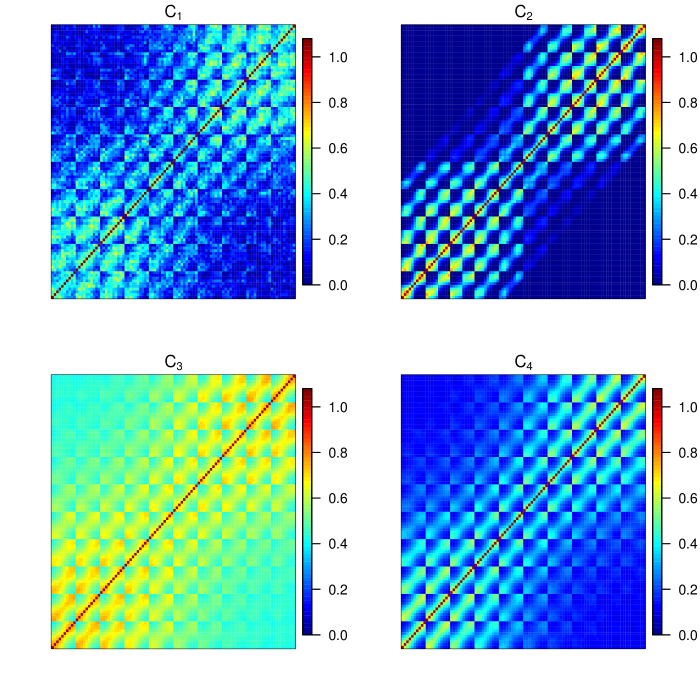
Figure 3: Pairwise probability matrix of two locations belong to the same cluster for a $10\times 10$ regular grid. $M=0.1$ for each cohesion

To better understand $M$’s influence on $\rho$’s cluster configuration a priori, we ran a small simulation study by drawing 5000 partitions from the sPPM for each of the four cohesions. The spatial configurations are regular $10\times 10$, $15\times 15$ and $20\times 20$ grids resulting in 100, 225, and 400 spatial locations. (We also considered the spatial configuration found in the application of Section 4.2 but results were similar and so are not provided.) The tuning parameters are set to the same values as used previously except that both $\alpha=1,2$ are considered for $C_{1}$. The results are provided in Table 2. Under the header $E(k_{n})$ are listed the number of clusters in $\rho$ averaged over the 5,000 prior draws, #sing denotes the number of singletons clusters and $\max|S_{j}|$ denotes the number of members in the largest cluster. Notice that setting $a=1.77$ for $C_{2}$ forces the sPPM to have at least 10 clusters. Also, as expected setting $\alpha=2$ results in $C_{1}$ producing more clusters. The number of clusters associated with $C_{1}$, $C_{2}$, and $C_{4}$ grow at a faster rate than $M\log((M+n)/M)$ while $C_{3}$ grows at a slower rate. The number of singleton clusters is also very reasonable for $M\leq 1$.

Table 2: Results from simulation study which drew 5,000 partitions from sPPM for each of the four cohesions.

		$n=100$			$n=225$			$n=400$
M	Method	$E(k_{n})$	#sing	$\max|S_{j}|$	$E(k_{n})$	#sing	$\max|S_{j}|$	$E(k_{n})$	#sing	$\max|S_{j}|$
$10^{-5}$	$C_{1_{\alpha=1}}$	1.00	0.00	100.00	1.00	0.00	224.99	1.01	0.00	399.99
	$C_{1_{\alpha=2}}$	3.91	0.03	37.06	4.61	0.01	66.85	4.98	0.00	106.92
	$C_{2}$	10.08	0.82	18.18	11.63	0.68	39.11	13.06	0.64	67.59
	$C_{3}$	1.00	0.00	100.00	1.00	0.00	225.00	1.00	0.00	400.00
	$C_{4}$	1.00	0.00	99.98	1.00	0.00	224.99	1.00	0.00	399.96
$10^{-4}$	$C_{1_{\alpha=1}}$	1.01	0.01	99.96	1.03	0.02	224.93	3.00	0.00	345.00
	$C_{1_{\alpha=2}}$	4.58	0.04	31.04	5.40	0.00	57.28	7.00	0.00	80.02
	$C_{2}$	10.11	0.81	18.20	11.65	0.68	39.13	13.08	0.64	67.53
	$C_{3}$	1.00	0.00	99.99	1.00	0.00	224.98	1.00	0.00	399.92
	$C_{4}$	1.00	0.00	99.97	1.00	0.00	224.90	1.00	0.00	399.86
$10^{-3}$	$C_{1_{\alpha=1}}$	1.16	0.03	99.37	2.17	0.00	141.19	2.77	0.00	227.96
	$C_{1_{\alpha=2}}$	5.50	0.00	25.76	6.76	0.00	49.19	8.08	0.00	68.10
	$C_{2}$	10.10	0.82	18.15	11.65	0.68	39.15	13.05	0.64	67.49
	$C_{3}$	1.00	0.00	99.93	1.00	0.00	224.85	1.01	0.00	399.52
	$C_{4}$	1.02	0.00	99.62	1.02	0.00	224.00	1.02	0.00	398.27
$10^{-2}$	$C_{1_{\alpha=1}}$	3.00	0.01	55.99	3.18	0.00	95.76	3.00	0.00	151.00
	$C_{1_{\alpha=2}}$	8.43	0.03	20.62	9.51	0.02	39.33	12.93	0.00	53.83
	$C_{2}$	10.17	0.84	18.13	11.72	0.70	39.10	13.20	0.65	67.30
	$C_{3}$	1.04	0.01	99.22	1.05	0.01	223.42	1.05	0.01	396.73
	$C_{4}$	1.16	0.01	96.33	1.17	0.01	217.12	1.19	0.01	385.04
$10^{-1}$	$C_{1_{\alpha=1}}$	5.91	0.22	30.66	8.87	0.00	46.20	8.50	0.02	83.57
	$C_{1_{\alpha=2}}$	14.12	0.73	13.78	18.98	0.63	22.30	25.03	0.31	32.20
	$C_{2}$	10.89	1.00	17.77	12.69	0.89	38.15	14.34	0.85	65.57
	$C_{3}$	1.42	0.07	92.84	1.46	0.07	209.11	1.51	0.07	370.28
	$C_{4}$	2.22	0.10	76.89	2.40	0.09	171.75	2.52	0.10	304.25
$10^{0}$	$C_{1_{\alpha=1}}$	14.96	1.11	14.24	21.66	0.63	22.48	31.03	1.21	31.20
	$C_{1_{\alpha=2}}$	26.50	2.57	7.85	43.98	3.27	11.70	54.80	1.74	16.78
	$C_{2}$	17.84	3.19	14.54	22.31	2.96	30.38	26.23	3.00	51.37
	$C_{3}$	4.27	0.72	62.99	4.64	0.70	141.88	5.01	0.71	249.55
	$C_{4}$	7.70	0.97	35.91	9.17	0.94	76.42	10.22	0.96	132.32
$10^{1}$	$C_{1_{\alpha=1}}$	36.51	9.28	7.06	60.10	9.61	10.12	85.77	10.31	13.30
	$C_{1_{\alpha=2}}$	52.34	19.55	4.46	92.38	19.91	6.68	137.61	19.82	7.87
	$C_{2}$	46.78	21.86	7.21	70.16	23.34	13.27	92.31	24.77	20.80
	$C_{3}$	18.83	6.59	25.10	23.02	6.80	56.47	25.86	6.89	99.96
	$C_{4}$	27.72	8.93	12.88	37.99	9.19	25.10	46.30	9.33	41.22

3.3 Modeling Spatial Structure via the Likelihood and Prior

Given $\rho$, the sky’s the limit on how spatial dependence might be modeled via the likelihood. A completely valid modeling strategy would be to assume independent observations given $\rho$. In this case, all spatial dependence would originate from the spatial clustering produced by the sPPM. Alternatively, global spatial structure or cluster specific spatial structure may be included in the likelihood producing much richer marginal spatial structure.

To explore spatial dependence further, we consider correlations among two observations as distance between them either increases to $\infty$ or decreases to $0$. This is done under a few likelihood models for each of the cohesions. Letting $\bm{y}=(y(\bm{s}_{1}),\ldots,y(\bm{s}_{n}))$, in the absence of spatial dependence in the likelihood, the basic model employed is

$$f(\bm{y}|\rho) =\prod_{h=1}^{k_{n}}f_{h}(\bm{y}^{\star}_{h})$$ (3.9)

$$Pr(\rho) \propto\prod_{h=1}^{k_{n}}C(S_{h},\bm{s}^{\star}_{h})$$

With $f_{h}(\bm{y}^{\star}_{h})=\int\prod_{i\in S_{h}}f(y(\bm{s}_{i})|\bm{\theta})dG_{0}(\bm{\theta})$ and $f(\cdot|\bm{\theta})$ denoting the likelihood and $G_{0}$ a prior on $\bm{\theta}$. Alternatively, the model can be written hierarchically using cluster labels $c_{1},\ldots,c_{n}$ in the following way

$$y(\bm{s}_{i})\mid\bm{\theta},c_{i} \stackrel{{\scriptstyle ind}}{{\sim}}f(\theta^{*}_{c_{i}}),\ \mbox{for}\ i=1,\dots,n$$

$$\theta^{*}_{\ell} \stackrel{{\scriptstyle iid}}{{\sim}}G_{0},\ \mbox{for}\ \ell=1,\ldots,k_{n}$$ (3.10)

with $\theta^{*}_{1},\ldots,\theta^{*}_{k_{n}}$ denoting cluster specific parameters so that $\theta_{i}=\theta^{*}_{c_{i}}$. In the spatial setting $c_{1},\dots,c_{n}$ are dependent multinomial latent variables with component probabilities derived from the sPPM.

When spatial structure is included in the likelihood it is done hierarchically by way of introducing spatial random effects, and models (3.9) and (3.3) will need to be adjusted accordingly. The spatial random effects can be cluster specific or global. If covariates are available, their relationship to the response can also be modeled as being cluster specific (local) or not (global). To simplify calculations in what follows we consider a Gaussian likelihood by setting $f(\cdot|\bm{\theta})=N(\cdot|\mu,\sigma^{2})$. Proofs to all Propositions are provided in the Appendix.

3.3.1 Covariances Under Local Regression

Proposition 3.1 furnishes the correlation between two observations available from a model that incorporates spatial information in the prior only. Therefore, all spatial structure is completely produced by the sPPM.

Proposition 3.1.

Let $\bm{x}(\bm{s}_{i})=\bm{x}_{i}$ and $y(\bm{s}_{i})=y_{i}$ denote a $p$-dimensional covariate vector and response at location $\bm{s}_{i}$. Further, let $\bm{\beta}^{*}_{1},\ldots,\bm{\beta}^{*}_{k_{n}}$ denote cluster specific parameters such that $\bm{\beta}^{*}_{h}\stackrel{{\scriptstyle iid}}{{\sim}}N(\bm{\mu},\bm{T})$ and assume that $\rho$ and $\{\bm{\beta}^{*}_{h}\}_{h=1}^{k_{n}}$ are mutually independent. Then under likelihood

$$y_{i}|\bm{x}_{i},{c}_{i},\bm{\beta}^{*},\sigma^{2}\sim N(\bm{x}^{\prime}_{i}\bm{\beta}^{*}_{c_{i}},\sigma^{2})$$ (3.11)

and a sPPM prior for $\rho$, the marginal correlation between two observations is

$$corr(y_{i},y_{j})=\dfrac{\bm{x}^{\prime}_{i}\bm{T}\bm{x}_{j}}{\sqrt{\bm{x}^{\prime}_{j}\bm{T}\bm{x}_{i}+\sigma^{2}}\sqrt{\bm{x}^{\prime}_{j}\bm{T}\bm{x}_{j}+\sigma^{2}}}Pr(c_{i}=c_{j}).$$ (3.12)

When $\bm{x}(\bm{s}_{i})=1$ for all $i$ (i.e., no covariates are available) and $\beta^{*}_{h}\stackrel{{\scriptstyle iid}}{{\sim}}N(\mu,\tau^{2})$, (3.12) simplifies to

$$corr(y_{i},y_{j})=\dfrac{\tau^{2}}{\tau^{2}+\sigma^{2}}Pr(c_{i}=c_{j}).$$ (3.13)

Remark 3.1.

Recall that as $d(\bm{s}_{i},\bm{s}_{j})\rightarrow\infty$, $Pr(c_{i}=c_{j})\rightarrow 0$ and therefore $corr(y_{i},y_{j})\rightarrow 0$. However, $corr(y_{i},y_{j})\not\rightarrow 1$ as $d(\bm{s}_{i},\bm{s}_{j})\rightarrow 0$. Although this result does not agree with many spatial covariance functions, it does agree with models that include a nugget effect. Additionally, from a clustering perspective it makes sense that locations allocated to same cluster are assigned the same parameter value, but not necessarily the same response value.

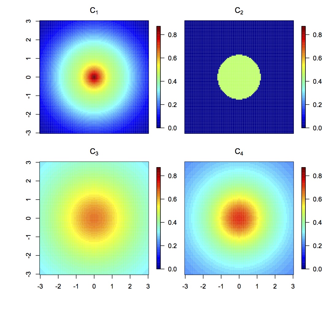
Figure 4: Correlations produced using (3.13) when two locations are considered. $\bm{s}_{1}$ is set to $(0,0)$ and $\bm{s}_{2}$ varies. The maximum correlation available is $\tau^{2}/(\tau^{2}+\sigma^{2})\approx 0.91$ with $\tau^{2}=1.0$ and $\sigma^{2}=0.1$

To visualize (3.13) as a function of distance $(d(\bm{s}_{1},\bm{s}_{2})=\|\bm{s}_{1}-\bm{s}_{2}\|)$, consider again the case of two locations. In Figure 4 we present correlations that are calculated by fixing $\bm{s}_{1}=(0,0)$ and moving $\bm{s}_{2}$ around in space. We set $\sigma^{2}=0.1$ and $\tau^{2}=1$ which produces $1/1.1\approx 0.9$ as the maximum correlation. For each cohesion we set $M=1$ and use the same values for the tuning parameters that were used in Section 3.2. The hard boundary of $C_{2}$ is evident as correlations produced by $C_{2}$ are either zero or $0.5(1/1.1)\approx 0.45$. The correlations associated with the other three cohesions decrease more smoothly as distances between $\bm{s}_{1}$ and $\bm{s}_{2}$ increase. It appears that correlations associated with $C_{1}$ decay quicker as distance increases relative to $C_{3}$ and $C_{4}$. The correlations associated with $C_{3}$ seem to be the most global in the sense that they decay slowly as a function of distance.

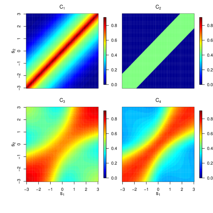
Figure 5: Pairwise correlations calculated using (3.13) and distances $|s_{1}-s_{2}|$. The maximum correlation available is $\tau^{2}/(\tau^{2}+\sigma^{2})\approx 0.91$ with $\tau^{2}=1.0$ and $\sigma^{2}=0.1$

In order to consider simultaneous movement between two observations, in Figure 5 $s_{1},s_{2}\in\mathbb{R}$ (rather than $\bm{s}_{1},\bm{s}_{2}\in\mathbb{R}^{2}$). Thus what is seen in Figure 5 are correlations associated with $d(s_{1},s_{2})=|s_{1}-s_{2}|$. Once again the maximum correlation is $1/1.1$. Just as in the previous figure, $C_{2}$’s hard boundary is evident and $C_{1}$ displays the most extreme correlation values. However, perhaps more interesting is the fact that the spatial structures produced by $C_{3}$ and $C_{4}$ appear to be non stationary and anisotropic as they are not constant in distance nor direction.

3.3.2 Correlations Under Local Regression and Global Spatial Structure

Proposition 3.2 provides the correlation between two observations from a model containing local regression and global spatial structure.

Proposition 3.2.

Let $\bm{x}_{i}$, $y_{i}$, and $\bm{\beta}^{*}_{1},\ldots,\bm{\beta}^{*}_{k_{n}}$ be as described in Proposition 3.1. Further, Let $\bm{\theta}=[\theta(\bm{s}_{1}),\ldots,\theta(\bm{s}_{n})]\sim GP(0,\lambda^{2}H(\phi))$ denote an $n$-dimensional vector of a spatial process where $GP(0,\lambda^{2}H(\phi))$ denotes a Gaussian process with covariance function $H(\phi):\mathbb{R}^{2}\times\mathbb{R}^{2}\rightarrow\mathbb{R}$ parametrized by $\phi$ and assume that $\rho$, $\{\bm{\beta}^{*}_{h}\}_{h=1}^{k_{n}}$, and $\bm{\theta}$ are mutually independent. Then for likelihood

$$y_{i}\mid\bm{x}_{i},\theta_{i},\bm{\beta}^{*},c_{i},\sigma^{2} \sim N(\bm{x}^{\prime}_{i}\bm{\beta}^{*}_{c_{i}}+\theta_{i},\sigma^{2})$$ (3.14)

and sPPM for $\rho$, the marginal correlation between two observations is

$$corr(y_{i},y_{j})=\frac{\lambda^{2}(H(\phi))_{i,j}+\bm{x}^{\prime}_{j}\bm{T}\bm{x}_{i}Pr(c_{i}=c_{j})}{\sqrt{\bm{x}^{\prime}_{i}\bm{T}\bm{x}_{i}+\lambda^{2}+\sigma^{2}}\sqrt{\bm{x}^{\prime}_{j}\bm{T}\bm{x}_{j}+\lambda^{2}+\sigma^{2}}}.$$ (3.15)

When $\bm{x}(\bm{s}_{i})=1$ for all $i$ (i.e., no covariates are available) and $\beta^{*}_{h}\stackrel{{\scriptstyle iid}}{{\sim}}N(\mu,\tau^{2})$, (3.15) simplifies to

$$corr(y_{i},y_{j})=\frac{\lambda^{2}}{\tau^{2}+\lambda^{2}+\sigma^{2}}(H(\phi))_{i,j}+\frac{\tau^{2}}{\tau^{2}+\lambda^{2}+\sigma^{2}}Pr(c_{i}=c_{j}).$$ (3.16)

Correlations are now a function of covariances from the GP and from spatial clustering. Notice that if the variability among cluster means $(\tau^{2})$ is large relative to $\sigma^{2}$ and $\lambda^{2}$, then cluster probabilities will be extremely influential in marginal correlations. Consider once again the simple case of two spatial locations. In this scenario if $d(\bm{s}_{1},\bm{s}_{2})\rightarrow\infty$, then $corr(y_{1},y_{2})\rightarrow 0$. While as $d(\bm{s}_{1},\bm{s}_{2})\rightarrow 0$, then $corr(y_{1},y_{2})\rightarrow(\lambda^{2}+\tau^{2}Pr(c_{1}=c_{2}))/(\lambda^{2}+\tau^{2}+\sigma^{2})$. Thus modeling spatial partitions with the sPPM results in decreased correlation for locations that have small probability of being co-clustered and an increase for those that have high probability relative to GP type spatial structures.

3.3.3 Covariances Under Global Regression and Local Spatial Structure

Proposition 3.3 provides the correlation between two observations for a model with local covariance structure and global regression.

Proposition 3.3.

Let $\bm{x}_{i}$, $y_{i}$ be as described in Proposition 3.1. Further let $\bm{\beta}\sim N(\bm{\mu},\bm{T})$ and $\bm{\theta}_{h}=\{\theta_{i}:i\in S_{h}\}$ such that $\bm{\theta}_{h}|\lambda_{h}^{2*},\phi^{*}_{h}\sim GP(0,\lambda^{2*}_{h}H(\phi^{*}_{h}))$. With out loss of generality order $\bm{\theta}=(\bm{\theta}_{1},\ldots,\bm{\theta}_{k_{n}})$ such that

$$\left(\begin{array}[]{c}\bm{\theta}_{1}\\ \vdots\\ \bm{\theta}_{k_{n}}\end{array}\right)\sim N_{n}\left(\bm{0},\left[\begin{array}[]{ccc}\lambda^{2*}_{1}H(\phi^{*}_{1})&\cdots&\bm{0}\\ \vdots&\ddots&\vdots\\ \bm{0}&\cdots&\lambda^{2*}_{k_{n}}H(\phi^{*}_{k_{n}})\end{array}\right]\right).$$ (3.23)

If spatial random effects (3.23) are combined with likelihood (3.14) and sPPM is employed to model $\rho$ with $\rho$, $\bm{\beta}$, and $\bm{\theta}$ being mutually independent, then the marginal correlation between two observations is

$$corr(y_{i},y_{j})=\dfrac{\bm{x}^{\prime}_{j}\bm{T}\bm{x}_{i}+cov^{*}(\theta_{i},\theta_{j})}{\sqrt{\sigma^{2}+\bm{x}^{\prime}_{i}\bm{T}\bm{x}_{i}+var^{*}(\theta_{i})}\sqrt{\sigma^{2}+\bm{x}^{\prime}_{j}\bm{T}\bm{x}_{j}+var^{*}(\theta_{j})}},$$ (3.24)

where $cov^{*}(\theta_{i},\theta_{j})=\sum_{h=1}^{k_{n}}\lambda^{2*}_{h}(H(\phi^{*}_{h}))_{i,j}Pr(c_{i}=c_{j}=h)$ and $var^{*}(\theta_{i})=\sum_{h=1}^{k_{n}}\tau^{2*}_{h}Pr(c_{i}=h)$. When $\bm{x}(\bm{s}_{i})=1$ for all $i$ (i.e., no covariates are available) and $\beta\sim N(\mu,\tau^{2})$, then (3.24) simplifies to

$$corr(y_{i},y_{j})=\dfrac{\tau^{2}+cov^{*}(\theta_{i},\theta_{j})}{\sqrt{\sigma^{2}+\tau^{2}+var^{*}(\theta_{i})}\sqrt{\sigma^{2}+\tau^{2}+var^{*}(\theta_{j})}}.$$ (3.25)

It is interesting to note that covariances are weighted averages of all cluster specific covariances with weights depending on distance. This type of spatial correlation structure is clearly nonstationary and nonisotropic.

4 Simulation Study and Examples

Except for very specific examples, the discussion to this point has been fairly generic with the idea of explaining different modeling approaches under a general framework. Now we provide more concrete illustrations by way of a small simulation study and a Chilean education application (with additional simulations and applications are provided in the Supplementary Material). The simulation studies and applications will require making some specific modeling assumptions but still within the general class of models thus far presented. To make methods invariant to scale of location, in the simulations and applications that follow we standardize $\bm{s}_{1},\dots,\bm{s}_{n}$ to have mean zero and unit variance. Fitting the models that will be described is a straightforward MCMC exercise. The algorithm we employ is based on MCMCSamplingMethodsForDPmixtureModels’s algorithm number 8 and details are provided in the Supplementary Material.

4.1 Simulation Study

We conduct a small simulation study to explore sPPM’s ability to recover partitions, make predictions and assess its goodness-of-fit performance. This is done by specifying the following model

$$y(\bm{s}_{i})|x(\bm{s}_{i}),c_{i},\mu^{*}_{c_{i}}(\bm{s}_{i}),\sigma^{2} \stackrel{{\scriptstyle ind}}{{\sim}}N(\mu^{*}_{c_{i}}(\bm{s}_{i})+x(\bm{s}_{i})\beta,\sigma^{2}),\ \sigma\sim UN(0,10),\,\beta\sim N(0,10^{2})$$ (4.1)

$$\mu_{h}^{*}(\bm{s}_{i}) \stackrel{{\scriptstyle iid}}{{\sim}}N(\mu_{0},\sigma^{2}_{0})\ \mbox{for}\ h=1,\ldots,k_{n}\ \mbox{and}\ \mu_{0}\sim N(0,10^{2}),\,\sigma_{0}\sim UN(0,10)$$

$$\{c_{i}\}_{i=1}^{n} \sim sPPM.$$

Here after this procedure will be referred to as the Conditional Model with Prior Spatial Structure (CPS). To the CPS we compare the spatial stick breaking (SSB) process found in SSB and a common spatial regression model (SR). More precisely,

1. The SR model refers to $y(\bm{s}_{i})|\bm{x}(\bm{s}_{i}),\bm{\beta},\theta(\bm{s}_{i})\sim N(\bm{x}^{\prime}(\bm{s}_{i})\bm{\beta}+\theta(\bm{s}_{i}),\sigma^{2})$ with $\bm{x}^{\prime}(\bm{s}_{i})=(1,x(\bm{s}_{i}))$, $\bm{\beta}=(\beta_{0},\beta_{1})\sim N_{2}(\bm{0},10^{2}\bm{I})$,   $[\theta(\bm{s}_{1}),\ldots,\theta(\bm{s}_{n})]\sim GP(0,\lambda^{2}H(\phi))$, and $\sigma^{2}\sim IG(a,b)$.

2. Given cluster labels $\{c_{i}\}_{i=1}^{n}$, SSB can be expressed as $y(\bm{s}_{i})|x(\bm{s}_{i}),c_{i},\mu^{*}_{c_{i}}(\bm{s}_{i}),\sigma^{2}\sim N(\mu^{*}_{c_{i}}(\bm{s}_{i})+x(\bm{s}_{i})\beta,\sigma^{2})$ where $c_{i}\sim Categorical(p_{1}(\bm{s}_{i}),\ldots,p_{m}(\bm{s}_{i}))$ with $p_{j}(\bm{s})=w_{j}(\bm{s})V_{j}\prod_{k<j}[1-w_{k}(\bm{s})V_{k}]$ for $V_{j}\stackrel{{\scriptstyle iid}}{{\sim}}beta(1,M)$. The $w_{j}(\bm{s})$ are location weighted kernels that introduce spatial dependence in the model (we always use a Gaussian kernel). Lastly, $\mu_{h}^{*}(\bm{s}_{i})\stackrel{{\scriptstyle iid}}{{\sim}}N(\mu_{0},\sigma^{2}_{0})\ \mbox{for}\ h=1,\ldots,k_{n}\ \mbox{and}\ \mu_{0}\sim N(0,10^{2}),\,\sigma_{0}\sim UN(0,10)$.

For the CPS we consider the four cohesions. For $C_{1}$ we set $\alpha=1$ and $\alpha=2$ and use the same tuning parameter values as in Section 3.2 for the other three cohesions functions.

The SSB is included because it is operationally very similar to the sPPM and was fit using the R function provided by SSB. Since the function only admits models that don’t include likelihood spatial structure, to make comparisons valid, we do not incorporate spatial structure in (4.1). The spBayes package in R (spBayes) was used to fit the SR model.

We considered the following four factors.

1. number of clusters (1, 4)

2. distribution of $\epsilon_{i}$ ($N(0,\sigma^{2})$ and $0.5N(0,\sigma^{2})+0.5N(1,\sigma^{2})$ with $\sigma^{2}=0.1$)

3. value of $M$

4. shapes of clusters (square, random)

The first factor was considered to assess clustering accuracy. Note the the sPPM and SSB will by definition create spatially referenced clusters, so we don’t expect high clustering accuracy when the number of clusters is 1. But including this level will allow us to assess the CPS when the true data generating mechanism is much simpler. Factors 2 and 3 are included to assess robustness of predictions and of goodness-of-fit against possible model perturbations. Factor 3 will only influence CPS and is included to investigate how calibrating sPPM is cohesion dependent.

To create synthetic data we employed the following as a data generating mechanism

$$y(\bm{s}_{i}) =\mu^{*}_{c_{i}}(\bm{s}_{i})+x(\bm{s}_{i})\beta+\theta(\bm{s}_{i})+\epsilon(\bm{s}_{i})$$

$$\bm{\theta}=[\theta(\bm{s}_{1}),\ldots,\theta(\bm{s}_{n})] \sim GP(\bm{0},\tau^{2}\bm{H}(\bm{\phi})).$$

An exponential covariance function with $\tau^{2}=2$ and $\phi=6$ was used to create $\bm{H}(\bm{\phi})$. Locations $(\bm{s}_{1},\ldots,\bm{s}_{n})$ were generated in two ways. The first method set $\bm{s}_{i}\stackrel{{\scriptstyle iid}}{{\sim}}UN(0,1)\times UN(0,1)$ with clusters being created by partitioning the $\mathbb{R}^{2}$ simplex into four equal area squares and assigning $\bm{s}_{i}$ accordingly. For the second method we set $\bm{s}_{i}\stackrel{{\scriptstyle iid}}{{\sim}}\sum_{k=1}^{4}0.25N(m,s^{2})$. The MixSim R function (see MixSim) was employed to generate locations from the mixture. For data containing four clusters, values of the cluster specific intercepts were $\bm{\mu}^{*}=(0,1,-1,-2)$. We set $\beta=1$ for all data sets and used $UN(0,10)$ to generate $x$ values. To obtain of point estimates for $\rho$ we employed the least squares procedure proposed in dahl:2006.

For each combination of factor levels $D=100$ data sets containing 100 training and 100 testing observations were generated. For each data set, the SSB, SR and sPPM procedures were fit to data by collecting 1000 MCMC iterates after discarding the first 1000. Results for $M=0.01$, $M=0.1$, and $M=1.0$ are presented in tabular form and can be found in Tables 3 and 4 (results for other values of $M$ are provided in the Supplementary Materials file). The columns of both tables correspond to the following

• RAND: represents the adjusted Rand index which measures proximity of estimated partition to the true partition. An adjusted Rand index close to 1 indicates a good match between estimated and true partition. The values found in the Table 3 are the adjusted Rand index averaged over the $D=100$ data sets.

• MSPE: represents the mean squared prediction error defined as $\frac{1}{100}\sum_{i=1}^{100}(Y_{p}(\bm{s}_{di})-\hat{Y}_{p}(\bm{s}_{di}))^{2}$ where $i$ indexes the 100 testing observations $(Y_{p}(s))$ and $\hat{Y}_{p}(\bm{s}_{id})=E(Y_{p}(\bm{s}_{di})|\bm{Y}(\bm{s}))$. This quantity measures the predictive performance of the models. The values found in Tables 3 and 4 are the MSPE averaged over the 100 data sets.

• LPML: represents the log pseudo marginal likelihood which is a goodness-of-fit metric (see WesJohnsonBook) that takes into account model complexity. The values in the two tables are average LPML over the 100 data sets.

Table 3: Simulation study results when data are generated with four clusters.

			$M=1.0$			$M=0.1$			$M=0.01$
Error	Cluster	Method	RAND	LPML	MSPE	RAND	LPML	MSPE	RAND	LPML	MSPE
Gaussian	Square	CPS $C_{1_{\alpha=1}}$	0.05	-169.73	2.75	0.09	-172.61	2.45	0.16	-178.07	2.43
		CPS $C_{1_{\alpha=2}}$	0.06	-183.36	2.47	0.12	-179.09	2.40	0.18	-180.24	2.26
		CPS $C_{2}$	0.16	-183.49	2.34	0.37	-182.49	2.24	0.49	-182.78	2.32
		CPS $C_{3}$	0.52	-183.21	2.37	0.50	-184.24	2.28	0.43	-184.09	2.41
		CPS $C_{4}$	0.29	-179.39	2.29	0.51	-180.74	2.18	0.59	-181.58	2.27
		SSB	0.15	-189.46	3.50	0.16	-190.22	3.37	0.13	-189.45	3.39
		SR	-	-2669.12	22.27	-	-2501.09	21.93	-	-2804.15	22.02
	Irregular	CPS $C_{1_{\alpha=1}}$	0.07	-166.78	2.55	0.14	-173.83	2.39	0.27	-176.76	2.28
		CPS $C_{1_{\alpha=2}}$	0.09	-176.04	2.42	0.17	-175.51	2.16	0.28	-177.87	2.11
		CPS $C_{2}$	0.25	-183.70	2.35	0.46	-183.52	2.30	0.52	-183.28	2.32
		CPS $C_{3}$	0.64	-181.00	2.24	0.58	-183.06	2.33	0.57	-182.55	2.30
		CPS $C_{4}$	0.63	-176.68	2.07	0.73	-178.89	2.13	0.74	-178.99	2.09
		SSB	0.20	-183.92	2.91	0.17	-183.73	2.86	0.19	-184.44	2.87
		SR	-	-2460.53	21.04	-	-2267.52	21.62	-	-2632.71	21.36
Mixture	Square	CPS $C_{1_{\alpha=1}}$	0.05	-169.89	2.62	0.09	-172.04	2.43	0.16	-176.90	2.36
		CPS $C_{1_{\alpha=2}}$	0.06	-179.92	2.54	0.11	-179.26	2.36	0.19	-178.36	2.18
		CPS $C_{2}$	0.16	-183.50	2.27	0.36	-181.42	2.24	0.47	-182.74	2.28
		CPS $C_{3}$	0.52	-183.27	2.25	0.47	-183.02	2.29	0.43	-184.64	2.35
		CPS $C_{4}$	0.29	-179.05	2.18	0.50	-179.88	2.18	0.57	-181.92	2.21
		SSB	0.16	-189.17	3.36	0.16	-189.33	3.40	0.15	-188.22	3.35
		SR	-	-2320.54	22.40	-	-2383.69	22.17	-	-2400.44	21.91
	Irregular	CPS $C_{1_{\alpha=1}}$	0.07	-170.99	2.61	0.17	-176.83	2.46	0.27	-176.37	2.27
		CPS $C_{1_{\alpha=2}}$	0.10	-179.31	2.40	0.18	-176.41	2.29	0.29	-176.05	2.20
		CPS $C_{2}$	0.22	-185.50	2.48	0.46	-184.50	2.41	0.54	-182.95	2.30
		CPS $C_{3}$	0.60	-183.57	2.33	0.56	-184.98	2.36	0.58	-182.77	2.27
		CPS $C_{4}$	0.61	-178.93	2.14	0.72	-180.52	2.13	0.77	-178.58	2.07
		SSB	0.18	-184.78	3.01	0.19	-185.32	2.98	0.19	-184.24	2.96
		SR	-	-2445.62	21.61	-	-2412.06	21.67	-	-2420.39	21.71

Table 3 provides results for data that contain four clusters. First notice that for $C_{1}$ the model fit associated with $CPS$ declines as $M$ decreases, but prediction accuracy and Rand index values improve. This indicates that $M$ must be small for $C_{1}$ or CPS tends to overfit by creating many clusters. For $C_{3}$ it appears that the opposite is true. Setting $\alpha=2$ for $C_{1}$ seems to reduce overfitting as model fit is slightly worse but out of sample prediction greatly improves. It seems like $C_{4}$ is the best at making accurate predictions regardless of the value of $M$, but selecting an appropriate $M$ is clearly cohesion dependent (something we explore more in the Supplementary Material). Interestingly CPS (and SSB) predict slightly better when error is a mixture and clusters are not regular. All that said, perhaps the main take home message is that CPS produces more accurate predictions and better data fit relative to SSB and SR for almost all data generating scenarios and cohesions.

Table 4 provides results for data with no clusters. Notice that we do not report the Rand index in this scenario as the CPS and SSB by construction create clusters. Because of this, as expected, the one cluster partition is not recovered well. That said, this scenario allows us to assess over-fit properties as the data structure is much simpler. It turns out that the model fits associated with data that contain no clusters are similar to those produced with data contained four clusters. However, the MSPE values are slightly better (which was expected). Generally speaking, it appears that CPS continues to perform well relative to SSB for each of the cohesions and SR (it is a bit surprising that SR does not perform much better).

Table 4: Simulation study results when data are generated with one cluster.

			$M=1.0$		$M=0.1$		$M=0.01$
Error	Cluster	Method	LPML	MSPE	LPML	MSPE	LPML	MSPE
Gaussian	Square	CPS $C_{1_{\alpha=1}}$	-168.99	2.06	-172.97	2.09	-174.82	2.08
		CPS $C_{1_{\alpha=2}}$	-171.94	2.01	-173.14	1.96	-172.66	1.92
		CPS $C_{2}$	-176.97	2.02	-177.12	2.07	-177.98	2.06
		CPS $C_{3}$	-178.06	2.07	-178.77	2.12	-179.18	2.15
		CPS $C_{4}$	-175.33	2.01	-176.70	2.05	-178.15	2.07
		SSB	-175.18	2.10	-176.30	2.13	-176.49	2.14
		SR	-2275.31	19.99	-2803.85	19.59	-2504.16	20.11
	Irregular	CPS $C_{1_{\alpha=1}}$	-165.90	1.98	-170.31	1.96	-174.71	1.95
		CPS $C_{1_{\alpha=2}}$	-168.86	1.88	-169.64	1.85	-170.12	1.76
		CPS $C_{2}$	-175.76	1.96	-174.65	1.95	-176.82	1.95
		CPS $C_{3}$	-176.33	1.98	-175.54	1.99	-177.61	2.01
		CPS $C_{4}$	-173.47	1.89	-173.52	1.94	-176.12	1.95
		SSB	-175.12	2.06	-174.91	2.07	-175.11	2.07
		SR	-1913.70	19.58	-1902.62	20.13	-2115.85	19.77
Mixture	Square	CPS $C_{1_{\alpha=1}}$	-172.31	2.14	-172.95	2.08	-176.83	2.01
		CPS $C_{1_{\alpha=2}}$	-179.92	2.00	-179.26	2.04	-178.36	1.97
		CPS $C_{2}$	-178.38	2.11	-177.22	2.04	-178.46	1.99
		CPS $C_{3}$	-179.00	2.15	-178.31	2.12	-179.95	2.06
		CPS $C_{4}$	-177.00	2.07	-176.30	2.02	-178.80	1.99
		SSB	-177.51	2.21	-176.22	2.17	-177.21	2.10
		SR	-2470.62	19.47	-2776.41	19.97	-2532.80	19.16
	Irregular	CPS $C_{1_{\alpha=1}}$	-168.59	2.00	-167.94	1.90	-172.75	1.96
		CPS $C_{1_{\alpha=2}}$	-168.61	1.84	-168.21	1.84	-170.23	1.81
		CPS $C_{2}$	-175.51	1.98	-173.57	1.90	-175.64	1.98
		CPS $C_{3}$	-176.13	2.00	-174.25	1.94	-176.14	2.01
		CPS $C_{4}$	-173.75	1.93	-172.53	1.88	-175.09	1.97
		SSB	-175.18	2.12	-173.83	2.02	-175.20	2.08
		SR	-2040.83	19.94	-2291.49	19.47	-1847.70	20.25

4.2 Application: Chilean Standardized Testing

Over the past 25 years Chile’s Ministry of Education has established a national large-scale standardized test called SIMCE (Sistema de Medición de la Calidad de la Educación, System Measurement of Quality of Education). It was introduced during the later part of the 80’s and since then has continually grown in scope and scale and is now a key component of Chilean educational policies (Meckes;Carrasco;2010; Manzi;Preiss;2013). During the early part of the 80’s education was privatized in Chile affording parents a great deal of flexibility when deciding to which school to send their children. One of the purported roles of SIMCE is to aid parents in making this decision. In addition to administrating the exam other socio-economic variables are recorded. Among them is mother’s education level which is known to influence individual SIMCE scores. Therefore, we include mother’s education as a covariate in modeling.

We briefly note that accommodating spatial dependence in education studies has only very recently been considered. In fact, the one article we found is Gelfand:2014. They explore regional differences in end of grade test scores in North Carolina using county level data. This was done by modeling reading and math scores jointly through a fairly sophisticated joint conditional autoregressive model.

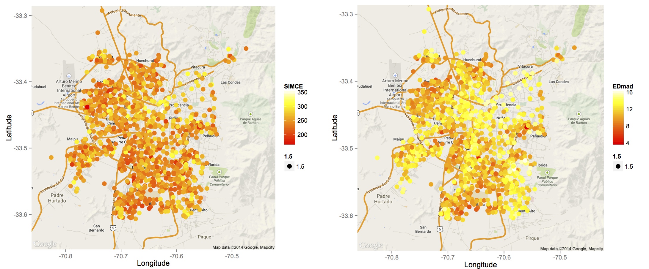
Figure 6: Spatial plots of SIMCE math scores and mother education level. The left figure corresponds with average SIMCE math scores, while the right average mothers education level.

We were given access to individual 2011 SIMCE 4th grade math scores. To simplify the analysis, instead of analyzing individual test scores and mother’s education level, we compute school-wide averages for both variables. The longitude and latitude of each school was recorded and we focus only on those schools that are located in the greater Santiago area (which produced 1215 schools). Figure 6 provides a spatial plot for both SIMCE and mother’s education values. Notice that schools in the north east part of the city tend to have higher SIMCE scores than those in the south and west. Mother’s education level also varies spatially with lower levels generally appearing in the west and south of Santiago. An exploratory analysis was performed to investigate spatial structures in the SIMCE data results of which are provided in the Supplementary Material.

To demonstrate the flexibility of pairing the sPPM with a variety of likelihoods, in what follows we detail and compare three reasonable models that could be proposed for the SIMCE data. In each case, SIMCE scores and mother’s education are standardized to have mean zero and unit standard deviation and the proposed model was fit to data by collecting 1000 MCMC iterates after discarding the first 10,000 as burn-in and thinning by 20. Convergence was monitored graphically. The MCMC chains mixed reasonably well and converged quickly.

To assess out of sample prediction, we divided the 1215 schools into 600 training observations and 615 testing observations. This partitioning of the data also facilitated a cross-validations study (see Supplementary Material) that in addition to information gleaned from the simulation study resulted in setting $M$ equal to $5\times 10^{-5}$, 0.1, 1.0, and 0.5 for cohesions 1-4 respectively. For $C_{1}$ both $\alpha=1$ and $\alpha=2$ were considered, but only results from $\alpha=1$ are reported as $\alpha=2$ produced very similar fits. The tuning parameters associated with other cohesions are those employed previously.

4.2.1 Conditional Model

In order to compare fits and predictions associated with sPPM to those of SSB, our first modeling approach is to model SIMCE scores conditional on mother education level with spatial structure in the prior only. This model corresponds to the CPS model of Section 4.1.

To compare model fit we once again employ LPML (see WesJohnsonBook), but now also include $MSE=\frac{1}{n}\sum_{i=1}(y(\bm{s}_{i})-\hat{y}(\bm{s}_{i}))^{2}$ and the Watanabe-Akaike information criterion (WAIC) which is a fairly new hierarchical model selection metric advocated in gelman:WAIC. The MSPE associated with the 615 testing observations is also provided under the “MSPE” column of Table 5. Excluding $C_{3}$, it appears that CPS fits the data better than SSB. Additionally, CPS appears to make more accurate predictions compared to SSB with $C_{4}$ producing the most accurate. CPS with $C_{1}$ clearly fits the data best and produces competitive predictions.

Table 5: Model fit comparisons associated with SIMCE test score data for sPPM and SSB

Procedure	WAIC	LPML	MSE	MSPE
CPS $C_{1}$	2113.64	-1314.21	0.12	0.533
CPS $C_{2}$	2420.56	-1358.97	0.21	0.535
CPS $C_{3}$	2739.73	-1364.31	0.48	0.538
CPS $C_{4}$	2706.71	-1361.58	0.40	0.516
SSB	2733.40	-1387.91	0.48	0.536

For the CPS procedure predicting an average SIMCE score for a completely new school requires knowing the new school’s location and mother’s education level. One approach would be to discretize mother’s education into, say, three levels and create a predictive map for each one. An alternative approach would be to first predict mother’s education level for the new school, then use the predicted mother’s education level as covariate to predict SIMCE. Using the later approach, the 600 training observations, and a regular grid of locations that belonged to the convex hull created by the observed school locations, we predict SIMCE scores by first predicting mother’s education level using a model similar to CPS but free of covariates. (i.e., $z(\bm{s}_{i})|\rho,\bm{\mu}^{*},\sigma^{2}\sim N(\mu_{c_{i}}^{*}(\bm{s}_{i}),\sigma^{2})$ where $z(\bm{s}_{i})$ denotes mother’s education level at the $i$th new school.) The predictive map of mother’s education values and SIMCE scores is provided in Figure 7 (we only report predictions from $C_{1}$ as the others were similar). The predicted values of mother’s education level and SIMCE math scores are completely plausible and the resulting spatial structure follows the general social-economic spatial distribution that is known to exist in Santiago.

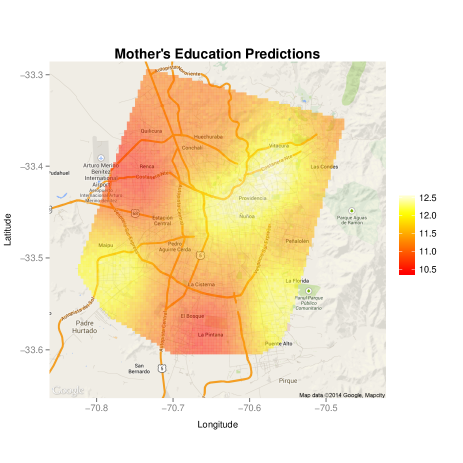
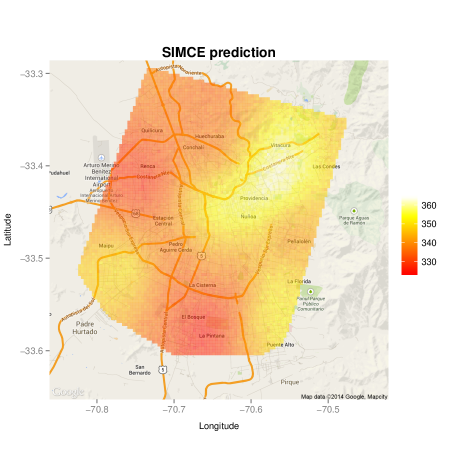
Figure 7: Predictive maps for mother’s education and SIMCE scores. The predicted mother’s education levels were used to predict SIMCE

4.2.2 Joint Model

Making predictions with the previous model is somewhat awkward as mother’s education needs to be either fixed or predicted using a completely different model. A more natural and coherent modeling approach for this application would be to model SIMCE scores and mother’s eduction jointly as both could be thought of as random quantities. To demonstrate flexibility in which sPPM can be incorporated in modeling and because comparisons to the SSB are not available for the joint model, we include spatial structure in the likelihood which amounts to using a simple coregionalization model (GelfandBook). Now let $\bm{y}(\bm{s}_{i})=[y_{1}(\bm{s}_{i}),y_{2}(\bm{s}_{i})]^{\prime}$ denote the $i$th school’s average SIMCE score and mother’s education level and consider the following data model

$$\bm{y}(\bm{s}_{i})=\bm{\mu}_{c_{i}}^{*}(\bm{s}_{i})+\bm{\theta}(\bm{s}_{i})+\bm{\epsilon}(\bm{s}_{i}),\quad i=1,\ldots,n,$$ (4.2)

where $\bm{\mu}_{c_{i}}^{*}(\bm{s}_{i})=[\mu_{1c_{i}}^{*}(\bm{s}_{i}),\mu_{2c_{i}}^{*}(\bm{s}_{i})]^{\prime}$ is a cluster specific 2-dimensional intercept vector whose spatial structure is guided through a sPPM prior, $\bm{\theta}(\bm{s}_{i})=(\theta_{1}(\bm{s}_{i}),\theta_{2}(\bm{s}_{i}))^{\prime}$ is a two-dimensional intercept whose spatial structure is directly incorporated into the likelihood in a manner that will be described shortly, and $\bm{\epsilon}(\bm{s}_{i})\sim N_{2}(\bm{0},\bm{\Sigma})$ is an error term. $\bm{\Sigma}$ contains dependence structure between SIMCE and mother’s education with variances denoted by $\sigma^{2}_{1}$ and $\sigma^{2}_{2}$ and covariance $\sigma_{12}=\eta\sigma_{1}\sigma_{2}$. For $h=1,\ldots,k_{n}$ we assume $\bm{\mu}_{h}^{*}(\bm{s}_{i})\stackrel{{\scriptstyle iid}}{{\sim}}N_{2}(\bm{\mu}_{0},\bm{T})$. To address spatial structure for each variable and the dependence that may exist between these two spatial processes, instead of modeling $\theta(\bm{s}_{i})$ and $\theta_{2}(\bm{s}_{i})$ directly with a Gaussian process we instead introduce $(\tilde{\theta}_{j}(\bm{s}_{1}),\tilde{\theta}_{j}(\bm{s}_{2}),\ldots,\tilde{\theta}_{j}(\bm{s}_{n}))\sim GP(\bm{0},\bm{C}_{j})$ independently for $j=1,2$ and set

$$\left(\begin{array}[]{c}\theta_{1}(\bm{s}_{i})\\ \theta_{2}(\bm{s}_{i})\end{array}\right)=\bm{A}\left(\begin{array}[]{c}\tilde{\theta}_{1}(\bm{s}_{i})\\ \tilde{\theta}_{2}(\bm{s}_{i})\end{array}\right)\ \mbox{where}\ \bm{A}=\left(\begin{array}[]{cc}1&\gamma\\ \gamma&1\end{array}\right),$$

for $\gamma\in(0,1)$. $\bm{C}_{j}$ of the Gaussian process denotes a valid covariance matrix constructed using an exponential covariance function. Thus, the $(\ell,\ell^{\prime})$th entry of $(\bm{C}_{j})$ is $(\bm{C}_{j})_{\ell,\ell^{\prime}}=\tau^{2}_{j}\exp\{-\phi_{j}\|\bm{s}_{\ell}-\bm{s}_{\ell^{\prime}}\|\}$. Prior distributions employed are $\tau^{2}_{j}\sim Gamma(1,1)$, $\phi_{j}\sim UN(0.5,30)$ (this implies a $UN(0.1,6)$ for effective range), $\bm{\mu}_{0}\sim N_{2}(\bm{0},10^{2}\bm{I})$, $\bm{T}\sim IW(2,\bm{I})$, and $\bm{\Sigma}\sim IW(2,\bm{I})$. We use $IW(\nu,\bm{\Lambda})$ to denote an inverse Wishart distribution with scale and matrix parameters $\nu$ and $\bm{\Lambda}$.

Under this model prediction of the SIMCE math score for a new school located at $\bm{s}_{0}$ is easily made via $y_{1}(\bm{s}_{0})|y_{2}(\bm{s}_{0})$ which has the following form

$$y_{1}(\bm{s}_{0})|y_{2}(\bm{s}_{0}) \sim N\left(\beta_{0c_{0}}^{*}(\bm{s}_{0})+\beta_{1}^{*}y_{2}(\bm{s}_{0}),\sigma^{2}_{1}(1-\eta^{2})\right),$$

with $\beta_{1}^{*}=\eta\frac{\sigma_{1}}{\sigma_{2}}$ and $\beta_{0c_{0}}^{*}(\bm{s}_{i})=\mu^{*}_{1{c_{0}}}+\theta_{1}(\bm{s}_{0})-\beta_{1}^{*}[\mu^{*}_{2{c_{0}}}+\theta_{2}(\bm{s}_{0})]$.

For this procedure to be useful, predictions of $\mu^{*}_{1{c_{0}}}$, $\mu^{*}_{2{c_{0}}}$, $\theta_{1}(\bm{s}_{0})$, $\theta_{2}(\bm{s}_{0})$, and $y_{2}(\bm{s}_{0})$ are needed. Values for $\mu^{*}_{1}$ and $\mu^{*}_{2}$ are readily available once $c_{0}$ is classified by way of the predictive distribution found Section 2 of the Supplementary Material (equation S.1). Values for $[\theta_{1}(\bm{s}_{0}),\theta_{2}(\bm{s}_{0})]$ are obtained by first predicting $[\tilde{\theta}_{1}(\bm{s}_{0}),\tilde{\theta}_{2}(\bm{s}_{0})]$ from $\tilde{\theta}_{1}(\bm{s}_{0})|\tilde{\theta}_{1}(\bm{s}_{1}),\ldots,\tilde{\theta}_{1}(\bm{s}_{n})$ and $\tilde{\theta}_{2}(\bm{s}_{0})|\tilde{\theta}_{2}(\bm{s}_{1}),\ldots,\tilde{\theta}_{2}(\bm{s}_{n})$ independently and then setting $[\theta_{1}(\bm{s}_{0}),\theta_{2}(\bm{s}_{0})]^{\prime}=\bm{A}[\tilde{\theta}_{1}(\bm{s}_{0}),\tilde{\theta}_{2}(\bm{s}_{0})]^{\prime}$. Finally, using the fact that $y_{2}(\bm{s}_{0})\sim N(\mu^{*}_{2{c_{0}}}+\theta_{2}(\bm{s}_{0}),\sigma^{2}_{2})$ a prediction for $y_{2}(\bm{s}_{0})$ is easily obtained. We will refer to the procedure just described as the Joint model with Likelihood Spatial Structure (JLS) model.

JLS can become computationally expensive as the number of schools grows. Incorporating spatial information solely in the prior would radically reduce computation time, but potentially at the cost of model fit. To investigate this trade off, we also consider

$$\bm{y}(\bm{s}_{i})|\bm{\mu}^{*},c_{i} \stackrel{{\scriptstyle ind}}{{\sim}}N_{2}(\bm{\mu}^{*}_{c_{i}}(\bm{s}_{i}),\bm{\Sigma})\ \mbox{for}\ i=1,\ldots,n\ \mbox{and}\ \bm{\Sigma}\sim IW(2,\bm{I})$$

$$\mu^{*}_{h}|\bm{\mu}_{0},\bm{T} \stackrel{{\scriptstyle iid}}{{\sim}}N_{2}(\bm{\mu}_{0},\bm{T})\ \mbox{with}\ \bm{T}\sim IW(2,\bm{I})$$

$$\bm{\mu}_{0} \sim N_{2}(\bm{0},10^{2}\bm{I})$$

$$\{c_{i}\}_{i=1}^{n} \sim sPPM.$$

As in the JLS, predictions at location $\bm{s}_{0}$ are also easily made via $E[y_{1}(\bm{s}_{0})|y_{2}(\bm{s}_{0})]=\mu_{1c_{0}}^{*}(\bm{s}_{0})+\eta\frac{\sigma_{1}}{\sigma_{2}}[y_{2}(\bm{s_{0}})-\mu_{2c_{0}}^{*}(\bm{s}_{0})]$. Values for $\mu_{1c_{0}}^{*}(\bm{s}_{0})$, $\mu_{2c_{0}}^{*}(\bm{s}_{0})$, and $y_{2}(\bm{s}_{0})$ are gathered using the procedure described for JLS. We will refer to this model as the Joint model with Prior Spatial Structure (JPS).

Table 6: Model fit comparisons for the JPS and JLS models fit to the SIMCE education data set.

Procedure	WAIC	LPML	MSE	MSPE	Clusters	Time
JPS $C_{1}$	2312.503	-1383.301	0.380	0.586	35.767	2154
JPS $C_{2}$	2569.589	-1438.750	0.415	0.590	34.746	4621
JPS $C_{3}$	2778.803	-1447.872	0.482	0.591	8.921	598
JPS $C_{4}$	2552.333	-1399.899	0.433	0.600	26.750	1090
JLS $C_{1}$	2047.319	-1291.011	0.244	0.574	34.992	38017
JLS $C_{2}$	2266.945	-1342.172	0.258	0.569	34.249	41022
JLS $C_{3}$	2553.984	-1376.176	0.365	0.573	6.789	38538
JLS $C_{4}$	2273.479	-1331.949	0.334	0.606	26.952	37565

Using the same $M$ values as in Section 4.2.1 we fit JLS and JPS to the training data and carried out prediction using the same grid of points and the testing data. Comparisons of the two joint models regarding model fit and computation time are provided in Table 6. The column “Clusters” is the expected number of clusters a posteriori and “Time” is the amount of computing time required to fit models (measured in seconds). MSPE is associated with the 600 testing observations. As expected fits using JLS are much better for all cohesion functions but at a substantial computational cost. However, JPS out of sample predictions are fairly competitive to those from JLS and may be considered if a timely answer is needed.

Maps associated with predictions made using JPS and JLS are provided in Figures 8 and 9. For JPS the four cohesions produce fairly different predictive surfaces, while for JLS the surfaces are very similar among the four cohesions. This illustrates that including spatial structure in the likelihood greatly impacts the predictive maps. For both procedures, the predictive maps identify the same general areas that contain higher SIMCE scores, but changes in SIMCE scores as a function of space are far more pronounced for JLS. This may be indicating that predictions are more local for JLS relative to JPS.

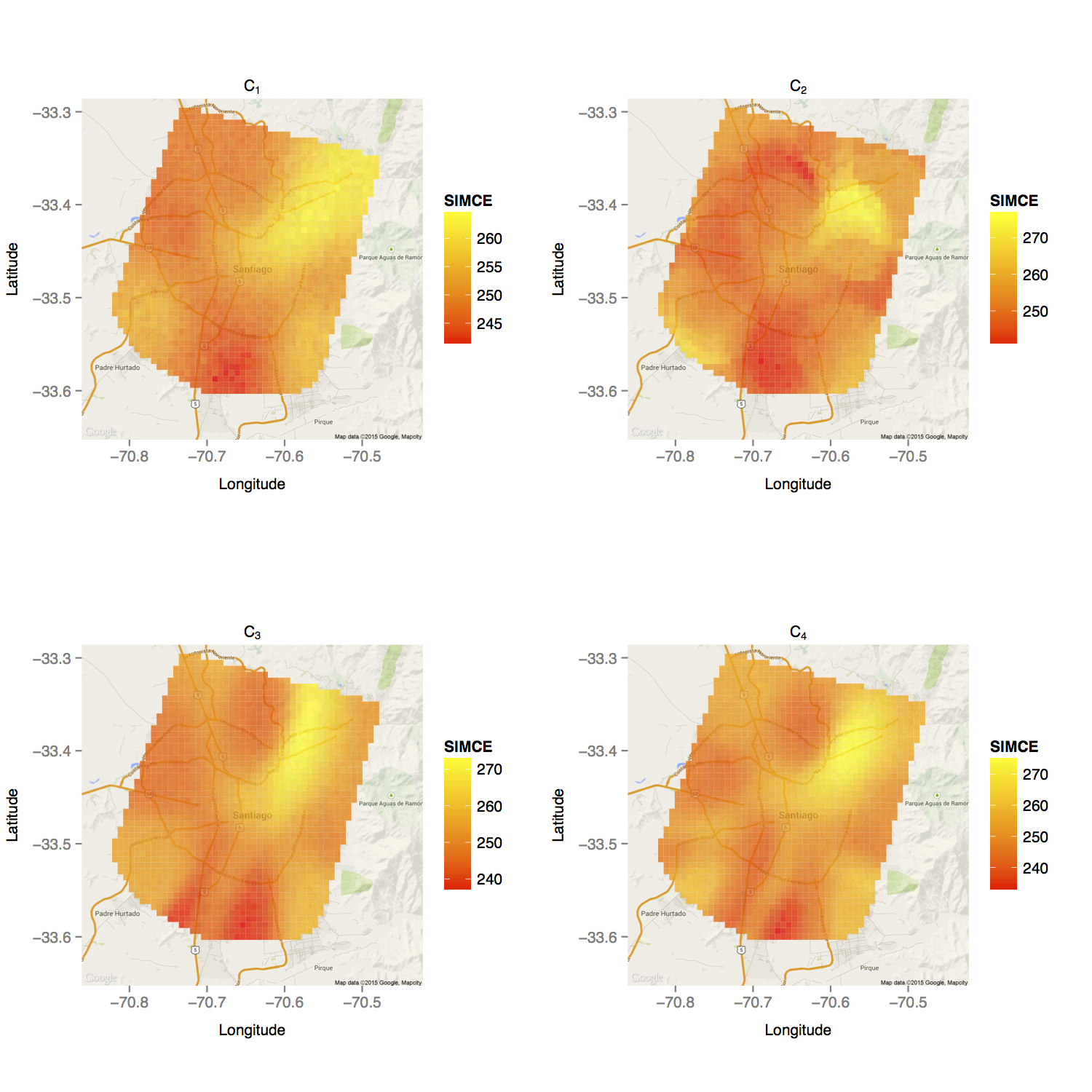
Figure 8: Predictive maps associated with JPS for each of the four cohesion functions

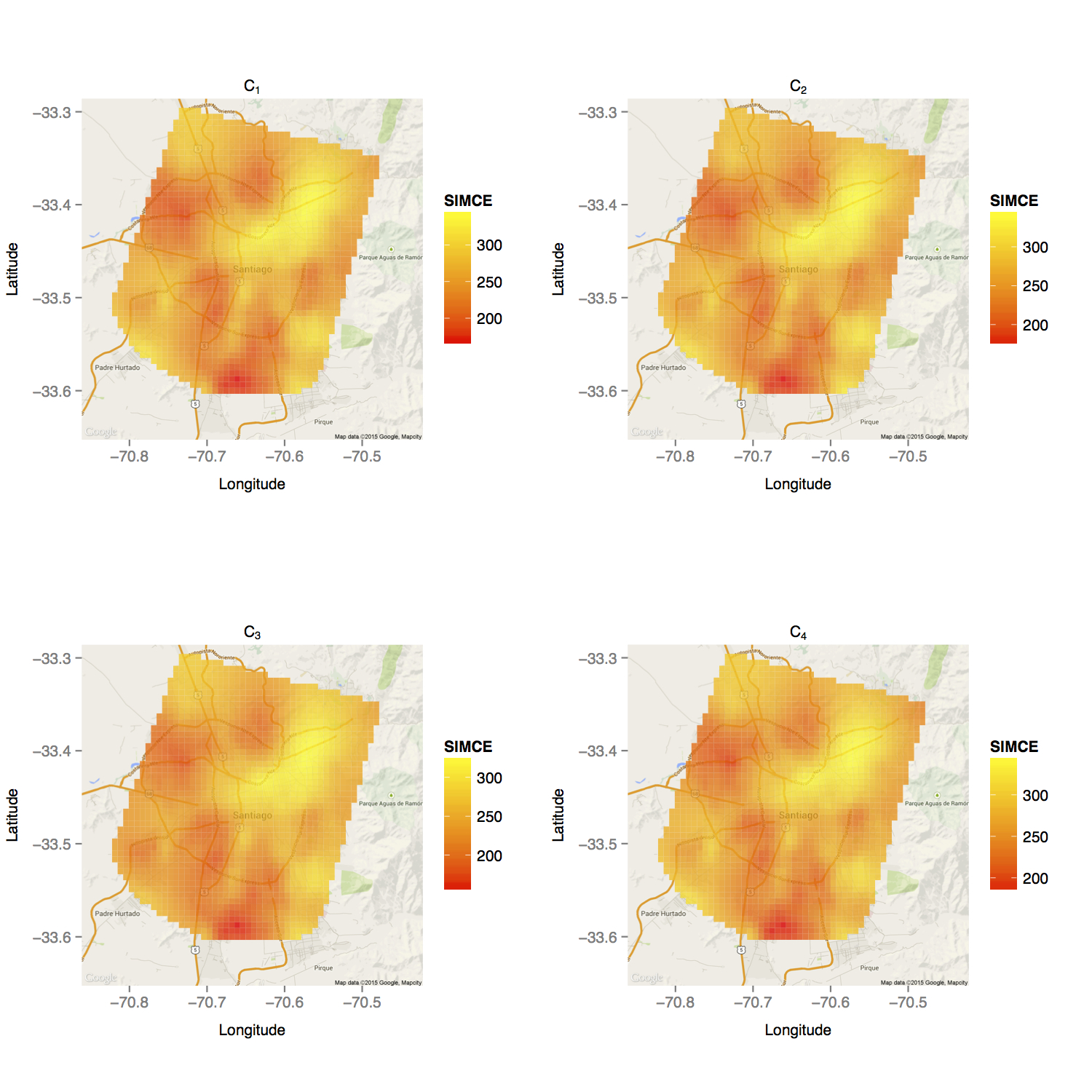
Figure 9: Predictive maps associated with JLS for each of the four cohesion functions

5 Conclusions

We have proposed a general procedure that extends PPMs to a spatial setting providing a mechanism to directly model the partitioning of locations into spatially dependent clusters. This mechanism in turn provides a means to introducing sophisticated spatial structures in modeling in a straightforward fashion. The cohesion function of the sPPM affords a great deal of flexibility regarding the type of spatial clusters available and the four that we have proposed are certainly not exhaustive. Other functions can be developed that produce different types of spatial structures. The simulation study and application showed that the methodology is particularly well suited for predictions and the fact that spatial information can be incorporated in the prior and likelihood allows for added flexibility in how spatial structure is modeled, providing the added benefit of capturing local structure. Exactly how to join local spatial structure so that global maps are smooth and continuous (if so desired) is a topic of ongoing research. Although not explicitly considered, including covariate information in the clustering mechanism in addition to spatial information should be a natural extension of work developed in PPMxMullerQuintanaRosner.

Appendix A Marginal Correlation Proof

We provide a detailed proof of Proposition 3.2 and 3.3. The proof of Proposition 3.1 follows very similar arguments.

A.1 Proof of Proposition 2

Proof.

From the law of total covariance

$$cov(y_{i},y_{j}) =cov_{\rho,\bm{\beta},\bm{\theta}}[E(y_{i}|\rho,\bm{\beta},\bm{\theta}),E(y_{j}|\rho,\bm{\beta},\bm{\theta})]+E_{\rho,\bm{\beta},\bm{\theta}}[cov(y_{i},y_{j},|\rho,\bm{\beta},\bm{\theta})]$$

$$=E_{\rho,\bm{\beta},\bm{\theta}}[(\bm{x}_{i}^{\prime}\bm{\beta}_{c_{i}}^{*}+\theta_{i})(\bm{x}_{i}^{\prime}\bm{\beta}_{c_{i}}^{*}+\theta_{i})]-E_{\rho,\bm{\beta},\bm{\theta}}[\bm{x}_{i}^{\prime}\bm{\beta}_{c_{i}}^{*}+\theta_{i}]E_{\rho,\bm{\beta},\bm{\theta}}[\bm{x}_{i}^{\prime}\bm{\beta}_{c_{i}}^{*}+\theta_{i}]+0$$

$$=E_{\rho,\bm{\beta},\bm{\theta}}[(\bm{x}_{i}^{\prime}\bm{\beta}_{c_{i}}^{*})(\bm{x}_{j}^{\prime}\bm{\beta}_{c_{j}}^{*})+(\bm{x}_{i}^{\prime}\bm{\beta}_{c_{i}}^{*})\theta_{j}+\theta_{i}(\bm{x}_{j}^{\prime}\bm{\beta}_{c_{j}}^{*})+\theta_{i}\theta_{i}]-E_{\rho,\bm{\beta}}[\bm{x}_{i}^{\prime}\bm{\beta}_{c_{i}}^{*}]E_{\rho,\bm{\beta}}[\bm{x}_{i}^{\prime}\bm{\beta}_{c_{i}}^{*}]$$

$$=E_{\rho,\bm{\beta}}[(\bm{x}_{i}^{\prime}\bm{\beta}_{c_{i}}^{*})(\bm{x}_{j}^{\prime}\bm{\beta}_{c_{j}}^{*})]+E_{\bm{\theta}}[\theta_{i}\theta_{i}]-E_{\rho,\bm{\beta}}[\bm{x}_{i}^{\prime}\bm{\beta}_{c_{i}}^{*}]E_{\rho,\bm{\beta}}[\bm{x}_{i}^{\prime}\bm{\beta}_{c_{i}}^{*}]$$

$$=\sum_{\rho}E_{\bm{\beta}}[tr\{\bm{\beta}^{*}_{c_{i}}\bm{x}_{i}\bm{x}^{\prime}_{j}\bm{\beta}^{*}_{c_{j}}\}]Pr(\rho)-\left(\sum_{\rho}E_{\bm{\beta}}[\bm{x}_{i}^{\prime}\bm{\beta}_{c_{i}}^{*}]Pr(\rho)\right)\left(\sum_{\rho}E_{\bm{\beta}}[\bm{x}_{j}^{\prime}\bm{\beta}_{c_{j}}^{*}]Pr(\rho)\right)+cov(\theta_{i},\theta_{j})$$

$$=\sum_{\rho}E_{\bm{\beta}}[tr\{\bm{x}_{i}\bm{x}^{\prime}_{j}\bm{\beta}^{*}_{c_{j}}\bm{\beta}^{*^{\prime}}_{c_{i}}\}]Pr(\rho)-\left(\sum_{\rho}\bm{x}_{i}^{\prime}\bm{\mu}Pr(\rho)\right)\left(\sum_{\rho}\bm{x}_{j}^{\prime}\bm{\mu}Pr(\rho)\right)+cov(\theta_{i},\theta_{j})$$

$$=\sum_{\rho:c_{i}=c_{j}}tr\{\bm{x}_{i}\bm{x}^{\prime}_{j}(\bm{T}+\bm{\mu}\bm{\mu}^{\prime})\}Pr(\rho)+\sum_{\rho:c_{i}\neq c_{j}}tr\{\bm{x}_{i}\bm{x}^{\prime}_{j}(\bm{\mu}\bm{\mu}^{\prime})\}Pr(\rho)-\bm{\mu}^{\prime}\bm{x}_{i}\bm{x}_{j}^{\prime}\bm{\mu}+cov(\theta_{i},\theta_{j})$$

$$=\bm{x}^{\prime}_{j}\bm{T}\bm{x}_{i}\sum_{\rho:c_{i}=c_{j}}Pr(\rho)+cov(\theta_{i},\theta_{j})$$

$$=\bm{x}^{\prime}_{j}\bm{T}\bm{x}_{i}Pr(c_{i}=c_{j})+\lambda^{2}(H(\phi))_{i,j}$$

Now using the law of total variance

$$var(y_{i}) =E_{\rho,\bm{\beta},\bm{\theta}}[var(y_{i}|\rho,\bm{\beta},\bm{\theta})]+var_{\rho,\bm{\beta},\bm{\theta}}[E(y_{i}|{\rho,\bm{\beta},\bm{\theta}})]$$

$$=E_{\rho,\bm{\beta},\bm{\theta}}[\sigma^{2}]+var_{\rho,\bm{\beta},\bm{\theta}}[\bm{x}_{i}^{\prime}\bm{\beta}_{c_{i}}^{*}+\theta_{i}]$$

$$=\sigma^{2}+\lambda^{2}+\bm{x}_{i}^{\prime}\bm{T}\bm{x}_{i}.$$

Using $corr(y_{i},y_{j})=\dfrac{cov(y_{i},y_{j})}{\sqrt{var(y_{i})}\sqrt{var(y_{j})}}$ completes the proof. ∎

A.2 Proof of Proposition 3

Proof.

Following similar arguments from the previous proof,

$$cov(y_{i},y_{j}) =cov_{\rho,\bm{\beta},\bm{\theta}}[E(y_{i}|\rho,\bm{\beta},\bm{\theta}),E(y_{j}|\rho,\bm{\beta},\bm{\theta})]+E_{\rho,\bm{\beta},\bm{\theta}}[cov(y_{i},y_{j},|\rho,\bm{\beta},\bm{\theta})]$$

$$=\bm{x}^{\prime}_{i}\bm{T}\bm{x}_{j}+\sum_{\rho:c_{i}=c_{j}}cov(\theta_{i},\theta_{j})Pr(\rho)+\sum_{\rho:c_{i}\neq c_{j}}cov(\theta_{i},\theta_{j})Pr(\rho)$$

$$=\bm{x}^{\prime}_{i}\bm{T}\bm{x}_{j}+\sum_{\rho:c_{i}=c_{j}}cov(\theta_{i},\theta_{j})Pr(\rho)$$

$$=\bm{x}^{\prime}_{i}\bm{T}\bm{x}_{j}+\sum_{h=1}^{k_{n}}\sum_{\rho:c_{i}=c_{j}=h}\lambda^{2}_{h}(H(\phi_{h}))_{i,j}Pr(\rho)$$

$$=\bm{x}^{\prime}_{i}\bm{T}\bm{x}_{j}+\sum_{h=1}^{k_{n}}\lambda^{2}_{h}(H(\phi_{h}))_{i,j}\sum_{\rho:c_{i}=c_{j}=h}Pr(\rho)$$

$$=\bm{x}^{\prime}_{i}\bm{T}\bm{x}_{j}+\sum_{h=1}^{k_{n}}\lambda^{2}_{h}(H(\phi_{h}))_{i,j}Pr(c_{i}=c_{j}=h)$$

And now using the law of total variance

$$var(y_{i}) =E_{\rho,\bm{\beta},\bm{\theta}}[var(y_{i}|\rho,\bm{\beta},\bm{\theta})]+var_{\rho,\bm{\beta},\bm{\theta}}[E(y_{i}|{\rho,\bm{\beta},\bm{\theta}})]$$

$$=\sigma^{2}+\bm{x}^{\prime}_{i}\bm{T}\bm{x}_{i}+\sum_{\rho}var_{\bm{\theta}}(\theta_{i})Pr(\rho)$$

$$=\sigma^{2}+\bm{x}_{i}^{\prime}\bm{T}\bm{x}_{i}+\sum_{h=1}^{k_{n}}var(\theta_{i})\sum_{\rho:c_{i}=h}Pr(\rho)$$

$$=\sigma^{2}+\bm{x}_{i}^{\prime}\bm{T}\bm{x}_{i}+\sum_{h=1}^{k_{n}}\tau^{2*}_{h}Pr(c_{i}=h)$$

Using $corr(y_{i},y_{j})=\dfrac{cov(y_{i},y_{j})}{\sqrt{var(y_{i})}\sqrt{var(y_{j})}}$ completes the proof. ∎