Imaging on a Sphere with Interferometers: the Spherical Wave Harmonic Transform

Abstract

I present an exact and explicit solution to the scalar (Stokes flux intensity) radio interferometer imaging equation on a spherical surface which is valid also for non-coplanar interferometer configurations. This imaging equation is comparable to $w$-term imaging algorithms, but by using a spherical rather than a Cartesian formulation this term has no special significance. The solution presented also allows direct identification of the scalar (spin 0 weighted) spherical harmonics on the sky. The method should be of interest for future multi-spacecraft interferometers, wide-field imaging with non-coplanar arrays, and CMB spherical harmonic measurements using interferometers.

1 Introduction

Basic radio interferometry deals with narrow fields-of-view measured by antenna elements constrained to a plane. Under such conditions, i.e. planar brightness distribution and planar visibility domain, the van Cittert-Zernike (vCZ) theorem (Thompson et al., 2001) states that the brightness and visibility distributions are two-dimensional Cartesian Fourier transforms of each other. An extension of the van Cittert-Zernike to arbitrarily wide fields and non-coplanar arrays was given in Carozzi and Woan (2009) where it was found that the simple Fourier transform relation no longer holds.

The generalized vCZ relation given in Carozzi and Woan (2009) is still similar to the original planar vCZ in that the brightness and visibility domains are ultimately expressed in Cartesian coordinates. A different approach to an interferometric relation for the full celestial sphere was given in Macphie and Okongwu (1975) which used spherical harmonics in the visibility domain. However the main result in that paper was a formula for point sources, i.e. the brightness distribution was given in terms of delta functions on the sphere. More recently, McEwen and Scaife (2008) used a spherical harmonic decomposition of visibility data to obtain the celestial sky multipole moments, but their treatment of the radial component of the visibility data was not made explicit.

In what follows I will provide a simple relation, analogous to the vCZ, between a brightness distribution on the celestial sphere and its visibility distribution in an arbitrary domain — possibly non-coplanar and not necessarily spherical — using a special case of the spherical Fourier-Bessel transform rather than using a Cartesian Fourier based transform.

The vCZ on a sphere relation presented here has several practical applications. Spherical harmonics of the sky temperature derived from interferometers is of current interest (Kim, 2007; Ng, 2001), and in the future there are plans for a multi-spacecraft interferometer mission. Such an interferometer would observe the full celestial sphere rather than a hemisphere, which limits Earth based interferometers. The results are also of interest to observations with non-coplanar arrays that currently must deal with the so-called $w$-term (Cornwell and Perley, 1992), which is a consequence of adapting the two-dimensional, Cartesian Fourier transform to work with three-dimensional visibility data to produce images of the celestial sphere. Although the imaging technique presented here is naturally suited to extended sources and multipole moments, also narrow field-of-view interferometers could benefit since, for high dynamic range imaging, the trend is to image the entire hemisphere anyways in order to handle leakage from beam side-lobes.

2 A relation between sky brightness on celestial sphere and non-coplanar visibilities

I start with the scalar intensity component of the extended vCZ theorem, i.e. a relation between visibility $\mathcal{V}$ and brightness $B$, as given in Carozzi and Woan (2009), valid on the celestial sphere, which can be written as

$$\mathcal{V}_{I}(\mathbf{r},k) =\int B_{I}(\Omega_{k})\exp\left(-\mathrm{i}\mathbf{k}\cdot\mathbf{r}\right)\mathrm{d}\Omega_{k}$$ (1)

where $\mathbf{r}$ is the position vector in the visibility domain, $\mathbf{k}$ is the wavevector and $\Omega_{k}=(\theta_{k},\phi_{k})$ are the angular components of $\mathbf{k}$ on the sphere. The subscripts $\bullet_{k}$ are used to denote that the angles refer to the spherical components of the wavevector. Since I will only be concerned with measurements in vacuum, the wavenumber $k=|\mathbf{k}|$ is equal the frequency used for the visibility measurements divided by the speed of light, $\omega/c$. Note that in eq. (1) the phase reference position is the origin. The subscript $\bullet_{I}$ in the equation above denotes the Stokes $I$ component, i.e. the scalar flux density. In what follows I discard the Stokes $I$ subscript as I will only deal with this component.

The expression (1) actually implies that $\mathcal{V}$ fulfills the Helmholtz equation, also known as the wave equation. This fact is not well appreciated in the radio interferometry literature, so I present it here. Operating with the Laplace operator on eq. (1), one finds that

$$\boldsymbol{\nabla_{r}}^{2}\mathcal{V}+k^{2}\mathcal{V}=0$$ (2)

which is the Helmholtz equation, or wave equation, in the visibility domain. The Helmholtz equation has, besides Cartesian solutions, also solutions in spherical coordinates, and this suggests that there should be a vCZ relation in terms of eigenfunctions of the spherical wave equation, which are equal to (Jackson, 1999)

$$j_{\ell}(kr)Y_{\ell m}(\theta,\phi),\quad\textrm{for }\ell=0,1,2,\ldots;\>m=-\ell,\ldots,\ell$$ (3)

where I invoke the boundary condition that the visibility should be finite at the origin. $Y_{\ell m}(\Omega)$ is the standard, orthonormal spherical harmonic function with $\ell,m$ corresponding to the polar and azimuthal quantal numbers respectively, and $j_{\ell}(kr)$ is the spherical Bessel function of the first kind. I will call these eigenfunctions spherical wave harmonics.

To fully convert eq. (1) into the eigenfunctions given in eq. (3), I proceed as follows. I use the plane wave decomposition formula, see Jackson (1999),

$$\mathrm{e}^{-\mathrm{i}\mathbf{k}\cdot\mathbf{r}}=4\pi\sum_{\ell=0}^{\infty}\sum_{m=-\ell}^{\ell}(-\mathrm{i})^{\ell}j_{\ell}(kr)Y_{\ell m}(\theta_{r},\phi_{r})Y_{\ell m}^{\ast}(\theta_{k},\phi_{k})$$ (4)

where the subscripts $\bullet_{r}$ denote the spherical coordinates of the visibility position vector $\mathbf{r}$ and $r=|\mathbf{r}|$. When this is inserted into eq. (1) it gives

$$\mathcal{V} =\int B(\Omega_{k})\left(4\pi\sum_{\ell=0}^{\infty}\sum_{m=-\ell}^{\ell}(-\mathrm{i})^{\ell}j_{\ell}(kr)Y_{\ell m}(\theta_{r},\phi_{r})Y_{\ell m}^{\ast}(\Omega_{k})\right)\mathrm{d}\Omega_{k}$$

$$=4\pi\sum_{\ell=0}^{\infty}\sum_{m=-\ell}^{\ell}(-\mathrm{i})^{\ell}j_{\ell}(kr)Y_{\ell m}(\theta_{r},\phi_{r})\int B(\Omega_{k})Y_{\ell m}^{\ast}(\Omega_{k})\mathrm{d}\Omega_{k}.$$ (5)

Then I expand the brightness distribution into spherical harmonics

$$B(\Omega_{k})=\sum_{\ell=0}^{\infty}\sum_{m=-\ell}^{\ell}b_{\ell m}Y_{\ell m}(\Omega_{k})$$ (6)

where $b_{lm}$ are the multipole moments of the sky. Inserting this back into eq. (5) one obtains

$$\mathcal{V}=4\pi\sum_{\ell=0}^{\infty}\sum_{m=-\ell}^{\ell}(-\mathrm{i})^{\ell}j_{\ell}(kr)Y_{\ell m}(\theta_{r},\phi_{r})\\ \times\int\left(\sum_{\ell=0}^{\infty}\sum_{m=-\ell}^{\ell}b_{\ell m}Y_{\ell m}(\Omega_{k})\right)Y_{\ell m}^{\ast}(\Omega_{k})\mathrm{d}\Omega_{k}\\ =4\pi\sum_{\ell=0}^{\infty}\sum_{m=-\ell}^{\ell}(-\mathrm{i})^{\ell}j_{\ell}(kr)Y_{\ell m}(\theta_{r},\phi_{r})b_{\ell m}$$ (7)

where I have used the orthogonality relation for the spherical harmonic functions

$$\int_{0}^{4\pi}Y_{\ell m}(\Omega)Y_{\ell^{\prime}m^{\prime}}^{\ast}(\Omega)\mathrm{d}\Omega=\delta_{\ell\ell^{\prime}}\delta_{mm^{\prime}}.$$ (8)

Finally I expand the visibility distribution into the spherical wave harmonics, eq. (3), with coefficients $\tilde{v}_{\ell m}$

$$\mathcal{V}=\sum_{\ell=0}^{\infty}\sum_{m=-\ell}^{\ell}\tilde{v}_{\ell m}j_{\ell}(kr)Y_{\ell m}(\Omega_{r}).$$ (9)

see Jackson (1999). Inserting this into the left-hand side of eq. (7), one obtains

$$\sum_{\ell=0}^{\infty}\sum_{m=-\ell}^{\ell}\tilde{v}_{\ell m}j_{\ell}(kr)Y_{\ell m}(\Omega_{r})\\ =4\pi\sum_{\ell=0}^{\infty}\sum_{m=-\ell}^{\ell}(-\mathrm{i})^{\ell}b_{\ell m}j_{\ell}(kr)Y_{\ell m}(\theta_{r},\phi_{r}).$$ (10)

From this equation, due to the orthonormality of the $Y_{\ell m}$ harmonics, one can identify that for any $(\ell,m)$,

$$\tilde{v}_{\ell m} =4\pi(-\mathrm{i})^{\ell}b_{\ell m}.$$ (11)

Eq. (11) is an important result, and shows that there is a simple proportionality relation between the brightness distribution, in terms of $b_{\ell m}$, and the visibility distribution, in terms of $\tilde{v}_{\ell m}$, with no integration or sum over any domain. The simplicity of this result is due to the fact that the spherical harmonic components are eigenfunctions of the measurement equation on the sphere (1) and that these components automatically fulfill the Helmholtz dispersion relation $k^{2}=\omega^{2}/c^{2}$. By contrast, the Cartesian Fourier transform consists of plane wave solutions, i.e. point sources, which are not eigenfunctions of the measurement equation on the sphere and do not automatically fulfill the dispersion relation which leads to the additional complexity of dealing with the $w$-term, i.e. the third and final wavevector component in the plane wave solutions.

McEwen and Scaife (2008) derived an essentially similar relationship to (11), albeit not explicitly. However, they did not provide an explicit scheme to derive the harmonic coefficients for an arbitrary array. In fact they speculated that a stable scheme could be developed, arguing that the presence of zeros of the spherical Bessel functions with large $\ell$ would complicate the recovery of the coefficients. I argue that the zeros of the spherical Bessel function for some $\ell$ simply mean that that particular $\ell$ does not contribute to the harmonic coefficient at that point, but e.g. the spherical Bessel functions with $\ell\pm 1$ will. In the next section I will show that the radial part of the visibility can indeed be incorporated into the recovery of the spherical harmonics of the sky, and later I will show that, at least for $\ell\leq 96$, it is possible to produce images comparable to those made with the Cartesian Fourier transform.

3 Computing the spherical wave harmonic coefficients of the visibility distribution

The result expressed in eq. (11) shows that spherical harmonic components of the celestial sky at a some frequency $\omega$ are proportional to a spherical Fourier-Bessel decomposition of the visibility distribution with the corresponding $k$. Although this vCZ relation is superficially simpler than the Cartesian Fourier transform, it still implies a comparable computational complexity since the $v_{\ell m}$ components need to be determined from the interferometric measurements.

In practice, an interferometer consists of an array of a finite number of antennas from which complex voltages are measured, and the visibilities are the complex powers obtained by cross-correlating between all antenna pairs. Thus $\mathcal{V}$ can only be sampled at a finite set of $Q$ measurements at points with spherical coordinates which I denote as $\left\{r_{i},\theta_{i},\phi_{i}\right\}_{i=1}^{Q}$. Note that from now on I will dispense with the $r$ subscripts for the spherical angles in the visibility domain that had been used in the previous section. Although there are no formal restrictions on the sampling distribution for the estimating the vCZ relation in the preceding section, certain distributions will be more advantageous than others.

A detailed discussion of the numerical implementation is outside the scope of the present paper, but a direct (non-gridded) naive solution for $\tilde{v}_{\ell m}$ can be derived as follows. Consider a visibility dataset $\mathcal{V}_{i}(k_{0})$ measured in narrow band with center frequency $\omega_{0}$ sampled at arbitrary positions. These can be seen as a sum of delta functions in the visibility domain

$$\mathcal{V}(k,r,\theta,\phi)=\sum_{i=1}^{Q}\mathcal{V}_{i}(k_{0})\delta(\mathbf{r}-\mathbf{r}_{i})\delta(k-k_{0})\\ =\sum_{i=1}^{Q}\frac{\mathcal{V}_{i}(k_{0})}{r^{2}\sin\theta}\delta(r-r_{i})\delta(\theta-\theta_{i})\delta(\phi-\phi_{i})\delta(k-k_{0})$$ (12)

where $k_{0}=\omega_{0}/c$ and the factor in the denominator is the normalization factor for the delta functions in spherical coordinates. The delta function in the $k$ domain is a simplifying approximation of the spectral density of the frequency band response function. Multiplying the right-hand side of eq. (12) with $j_{\ell}(k_{0}r)Y_{\ell m}^{\ast}(\theta,\phi)$, and then integrating this over a spherical volume that bounds the visibility domain results in

$$\int_{0}^{\infty}\!\!\int_{0}^{\pi}\!\!\int_{0}^{2\pi}\sum_{i=1}^{Q}\frac{\mathcal{V}_{i}(k)}{r^{2}\sin\theta}j_{\ell}(k_{0}r)Y_{\ell m}^{\ast}(\theta,\phi)\delta(r-r_{i})\delta(\theta-\theta_{i})\delta(\phi-\phi_{i})\\ \times\delta(k-k_{0})r^{2}\sin\theta\,\mathrm{d}r\mathrm{d}\theta\mathrm{d}\phi=\sum_{i=1}^{Q}\mathcal{V}_{i}(k_{0})j_{\ell}(k_{0}r_{i})Y_{\ell m}^{\ast}(\theta_{i},\phi_{i})\delta(k-k_{0}).$$ (13)

For the left-hand side of eq. (12), I insert eq. (9) and do exactly the same the steps as were performed on the right-hand side and then get

$$\int_{0}^{\infty}\!\!\int_{0}^{\pi}\!\!\int_{0}^{2\pi}\sum_{\ell^{\prime}=0}^{\infty}\sum_{m^{\prime}=-\ell^{\prime}}^{\ell^{\prime}}\tilde{v}_{\ell^{\prime}m^{\prime}}j_{\ell^{\prime}}(kr)Y_{\ell^{\prime}m^{\prime}}(\theta,\phi)j_{\ell}(k_{0}r)Y_{\ell m}^{\ast}(\theta,\phi)\\ \times r^{2}\sin\theta\,\mathrm{d}r\mathrm{d}\theta\mathrm{d}\phi=\sum_{\ell=0}^{\infty}\sum_{m=-\ell}^{\ell}\tilde{v}_{\ell m}\intop_{0}^{\infty}j_{\ell}(kr)j_{\ell}(k_{0}r)r^{2}\,\mathrm{d}r\\ =\sum_{\ell=0}^{\infty}\sum_{m=-\ell}^{\ell}\tilde{v}_{\ell m}\frac{\pi\delta(k-k_{0})}{2k_{0}^{2}}$$ (14)

where I have used the relation

$$\int_{0}^{\infty}j_{\ell}(kr)j_{\ell}(k_{0}r)r^{2}\,\mathrm{d}r=\frac{\pi\delta(k-k_{0})}{2k_{0}^{2}}$$ (15)

which is valid for all $\ell$, see Leistedt et al. (2012). Integrating both the left- and right-hand sides, i.e. the last results of eq. (14) and eq. (15), over all $k$ and equating these two results I find that

$$\tilde{v}_{\ell m}(k_{0})=\frac{2k_{0}^{2}}{\pi}\sum_{i=1}^{Q}\mathcal{V}_{i}(k_{0})j_{\ell}(k_{0}r_{i})Y_{\ell m}^{\ast}(\theta_{i},\phi_{i}).$$ (16)

This my main result in terms of providing an explicit, direct quadrature rule for computing the spherical wave coefficients from arbitrarily placed visibility samples. Note that there is no formal restriction on the radial positions of the samples, for instance with respect to the zeros of the spherical Bessel functions.

The transform used above to derive eq. (16) is a type of spherical Bessel-Fourier decomposition, see Leistedt et al. (2012); Baddour (2010). But a crucial difference is that, in the present work, the radial component of the wavevector, i.e. the wavenumber $k$, is already known since radio interferometric visibility data is almost always given as functions of frequency in narrow bands, hence the delta function in $k$. Thus the transform is two-dimensional rather than three-dimensional for a given frequency. For this reason it may be more appropriate to call this something else instead, so I will use the term spherical wave harmonic transform (SWHT).

4 All-sky imaging examples

In this section I apply the SWHT to real radio interferometer data to illustrate the imaging technique. I used data from the Swedish LOFAR station, known as SE607, in particular the Low Band Array (LBA), which is a ~60 m diameter array of 96 crossed dipoles placed in a pseudo-random, co-planar pattern covering the frequency range $10-90$ MHz.

The dataset I used was a snap-shot, i.e. the cross-correlations (and auto-correlations) are integrated over a short, 10 s, time interval, so that the array can be taken to be co-planar. This was chosen since it then can be compared with the ordinary (non-gridded) Cartesian Fourier transform. The data was for center frequency 37.1 MHz in a 192 kHz wide band. I applied eq. (16) to the visibility data and computed the $\tilde{v}_{\ell m}$ coefficients up to $\ell=L_{\textrm{max}}=96$, which matches the number of elements. These coefficients were then converted to the sky harmonic coefficients $b_{\ell m}$ using eq. (11), and then these coefficients were used to generate an image through eq. (6).

The result of this SWHT technique is shown in Figure 1, subplot a). For comparison, subplot b) shows the ordinary Cartesian Fourier transformed image, also known as a dirty image, and subplot c) shows a reference model at the slightly higher frequency of 50 MHz and with better resolution. It is clear from this Figure that the SWHT is very similar to the Cartesian Fourier transform. The main difference is the presence of emissions beyond the telescope horizon, i.e. directions apparently below 0 elevation, for instance in the South-East corner of subplot b). These emissions are an erroneous artifact of the two-dimensional Cartesian Fourier imaging technique, since the two Cartesian Fourier components, or direction cosines, go from -1 to +1, and there is nothing to stop components with absolute value greater than 1 from contributing to the image. In other words, this illustrates the fact that the Cartesian Fourier transform does not automatically fulfill the dispersion relation $k^{2}=\omega^{2}/c^{2}$, as already mentioned.

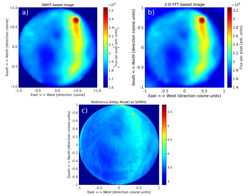
Figure 1: Orthographically projected images of Stokes $I$ flux in arbitrary units of the celestial hemisphere over LOFAR SE607 LBA on 3 December 2014, 00:16 UT. The subplot a) image was computed using the spherical Bessel harmonics with $\max(\ell)=96$ at 37.1 MHz. The subplot b) image was computed using a non-gridded two-dimensional Fourier transform also at 37.1 MHz. Subplot c) is an reference model image at 50 MHz. The extended emission in the West is the Milky Way. The strong point source in the North-West is Cassiopeia A. Emission from the galactic North spur can be seen in the North-East. The circle suggested in these images is the telescope local horizon at elevation 0. Note that neither of the images a) or b) have been compensated for the antenna gain pattern.

The run times were slower for the SWHT, but these could be improved up by using fast spherical harmonic transform algorithms, such as Rokhlin and Tygert (2006), which have computation time complexity of the order $\mathcal{O}(N^{2}\log N)$, where $N$ is the number of sample points. It is possible that an SWHT algorithm could be constructed to have a time complexity not much greater than this, making it comparable to the $w$-term imaging algorithms.

5 Conclusions

I have derived a vCZ relation, eq. (11), between a spherical brightness distribution and an unconstrained visibility distribution. I have also presented the SWH transform of the visibility data to compute the spherical harmonics of the sky from which images can be made. This technique was shown to be capable of producing images comparable to ordinary dirty images. It should be useful for radio inferometric imaging of extended sources or for determining multipole moments of the celestial sky. It extends naturally to visibility data from non-coplanar arrays, and thus the technique is comparable to $w$-term imaging methods.

References

- Baddour (2010) Natalie Baddour. Operational and convolution properties of three-dimensional fourier transforms in spherical polar coordinates. JOSA A, 27(10):2144–2155, 2010.
- Carozzi and Woan (2009) T. D. Carozzi and G. Woan. A generalized measurement equation and van Cittert-Zernike theorem for wide-field radio astronomical interferometry. Monthly Notices of the Royal Astronomical Society, 395(3):1558–1568, May 2009. doi: 10.1111/j.1365-2966.2009.14642.x. URL http://dx.doi.org/10.1111/j.1365-2966.2009.14642.x.
- Cornwell and Perley (1992) T. J. Cornwell and R. A. Perley. Radio-interferometric imaging of very large fields - The problem of non-coplanar arrays. Astronomy and Astrophysics, 261:353–364, July 1992.
- Jackson (1999) John D. Jackson. Classical Electrodynamics. Wiley & Sons, Inc., New York, NY …, third edition, 1999. ISBN 0-471-30932-X.
- Kim (2007) Jaiseung Kim. Direct reconstruction of spherical harmonics from interferometer observations of the cosmic microwave background polarization. Monthly Notices of the Royal Astronomical Society, 375(2):625–632, 2007. doi: 10.1111/j.1365-2966.2006.11285.x. URL http://mnras.oxfordjournals.org/content/375/2/625.abstract.
- Leistedt et al. (2012) B. Leistedt, A. Rassat, A. Réfrégier, and J.-L. Starck. 3dex: a code for fast spherical fourier-bessel decomposition of 3d surveys. A&A, 540:A60, 2012. doi: 10.1051/0004-6361/201118463. URL http://dx.doi.org/10.1051/0004-6361/201118463.
- Macphie and Okongwu (1975) Robert H. Macphie and E. H. Okongwu. Spherical harmonics and earth-rotation synthesis in radio astronomy. Antennas and Propagation, IEEE Transactions on, 23(3):386–391, 1975.
- McEwen and Scaife (2008) J. D. McEwen and A. M. M. Scaife. Simulating full-sky interferometric observations. Monthly Notices of the Royal Astronomical Society, 389(3):1163–1178, 2008. doi: 10.1111/j.1365-2966.2008.13690.x. URL http://mnras.oxfordjournals.org/content/389/3/1163.abstract.
- Ng (2001) Kin-Wang Ng. Complex visibilities of cosmic microwave background anisotropies. Phys. Rev. D, 63:123001, May 2001. doi: 10.1103/PhysRevD.63.123001. URL http://link.aps.org/doi/10.1103/PhysRevD.63.123001.
- Rokhlin and Tygert (2006) Vladimir Rokhlin and Mark Tygert. Fast algorithms for spherical harmonic expansions. SIAM Journal on Scientific Computing, 27(6):1903–1928, 2006.
- Thompson et al. (2001) A. Richard Thompson, M. Moran Moran, and George W. Jr Swenson. Interferometry and Synthesis in Radio Astronomy. John Wiley & Sons, Inc., 2001.