Stability threshold approach for complex dynamical systems

Abstract

A new measure to characterize stability of complex dynamical systems against large perturbation is suggested, the stability threshold (ST). It quantifies the magnitude of the weakest perturbation capable to disrupt the system and switch it to an undesired dynamical regime. In the phase space, the stability threshold corresponds to the “thinnest site” of the attraction basin and therefore indicates the most “dangerous” direction of perturbations. We introduce a computational algorithm for quantification of the stability threshold and demonstrate that the suggested approach is effective and provides important insights. The generality of the obtained results defines their vast potential for application in such fields as engineering, neuroscience, power grids, Earth science and many others where robustness of complex systems is studied.

Introduction

Complex systems science is strongly based on linear stability analysis considering small perturbations of dynamical systems. In a seminal paper PC1998 this concept was extended even to the stability of synchronization in complex networks leading to the efficient master stability formalism. However, for various applications often the influence of large perturbations is also of crucial importance. Typical examples are climatological systems, in particular ocean circulations. Well accepted is that the Atlantic Meridional Overturning Circulation may be sensitive to changes in the freshwater balance of the northern North Atlantic. When an anomalous freshwater flux is applied in the subpolar North Atlantic, this circulation collapses in many ocean-climate models MOC . Another example is power grids which are networks of connected generators and consumers of electrical power. For proper function of such networks synchronization between all the nodes is essential. Local failures, overloads or lines breaks may cause desynchronization of nodes and lead to large-scale blackouts Ewart78 ; Machovski2008 .

The study of system’s stability against large perturbations implies treating the following challenging problem: definition of the class of “safe”, or admissible perturbations after which the system returns back to the initial regime. In contrast, “unsafe” perturbations switch the system to another, often unwanted, dynamical regime. The definition of the class of safe perturbations of a nonlinear system is very complicated and basically different from the linear stability analysis. The reason is that for large perturbations linearization is inadequate and the perturbed dynamics is governed by nonlinear equations whose analytical study is impossible in general. Some analytical methods do exist, for example the method of Lyapunov functions Lyap . However, this method has serious limitations since a Lyapunov function for a particular dynamical system is often not constructive. The “safe” perturbation class can also be analytically estimated for some specific systems, e.g. networks of spiking neurons Timme . Nevertheless, an important task is to develop numerical methods of defining and describing the class of safe perturbations Wiley2006 .

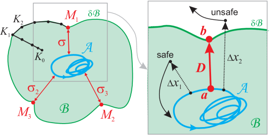
Figure 1: Stability threshold (ST) and its quantification. Attractor $\mathcal{A}$, its attraction basin $\mathcal{B}$ and ST $\sigma$. The trace of the algorithm converging to the point $M$ is shown by black dots. Other LOCT points $M_{2}$ and $M_{3}$ are also shown. In the the zoomed part, safe and unsafe perturbations are shown. Dotted lines are perturbations, solid black lines are trajectories of the perturbed system.

From the viewpoint of nonlinear dynamics, established dynamical regimes of the system corresponds to attractors in the phase space. The class of safe perturbations is equal to the attraction basin, i.e. the set of the points which converge to the attractor. A perturbation is safe if it brings the system to a point within the attraction basin. The first attempt to characterize attraction basins in complex networks was undertaken in BS where the concept of basin stability was introduced. The basin stability equals

$$S_{B}=\int_{Q}\chi(x)\rho(x)dx,$$ (1)

where $Q$ is the set of possible perturbed states $x$, $\rho(x)$ with $\int_{Q}\rho(x)dx=1$ is the density of the perturbed states, and $\chi(x)$ equals one if the point $x$ converges to the attractor and zero otherwise. The value $S_{B}\in(0;1]$ expresses the likelihood that the perturbed system returns to the attractor. An important advantage of this measure is that it can be easily calculated by Monte-Carlo method. Namely, one should just take a large number of random points in the phase space and check how many of them converge to the attractor. If $M$ of $N\gg 1$ points converge, $S_{B}\approx M/N$.

Basin stability is an important characteristic extending the concept of linear stability for the case of large perturbations. However, many real dynamical systems, especially complex networks, possess highly-dimensional phase space with complicated structure. This makes it problematic to characterize an attraction basin by just a single scalar value. Moreover, basin stability depends on the perturbation class $Q$ which should be chosen a priory.

In this paper we suggest a new measure to characterize stability against large perturbation, the stability threshold (ST). We were inspired by the observation that for real systems it is often important to know the maximal magnitude of perturbation which the system is guaranteed to withstand, like the maximal voltage jump for a stabilizer or the maximal bullet energy for a bulletproof vest. In the following, in Sec. 1 we introduce the ST in detail and explain how to calculate it. In Sec. 2 and 3 its potential is demonstrated for two paradigmatic model systems. In Sec. 4 we relate the two measures, the stability threshold and the basin stability. In Sec. 5 we briefly summarize and discuss our results.

I Definition and quantification of stability threshold

We define ST as the minimal magnitude of a perturbation capable to disrupt the established dynamical regime, i.e. to push the system out of the attraction basin. In the phase space, ST is the minimal distance between the attractor $\mathcal{A}$ and the border $\mathcal{\delta B}$ of its attraction basin, i.e.

$$\sigma=\inf\left\{\mbox{dist}(a,b)\,|a\in\mathcal{A},\,b\in\mathcal{\delta B}\right\},$$ (2)

where $\mbox{dist}(\cdot,\cdot)$ is the distance between the points in the phase space. Further, we use Euclidean metric to calculate the distance. However, any other metrics can be used as well.

To better understand the physical meaning of ST consider the system settled to the attractor $\mathcal{A}$ as depicted in Fig. 1. Let $\,a\in\mathcal{A}$ and $b\in\mathcal{\delta B}$ be points corresponding to ST such that $\mbox{dist}\left(a,b\right)=\sigma$. Consider now a perturbation of the system which results in a quick change of its state. Namely, let the system state change from the unperturbed one $x_{u}$ to the perturbed one $x_{p}$ so that the perturbation $\Delta x=x_{p}-x_{u}$ has the magnitude $q=|\Delta x|$ . If $q<\sigma$, the perturbation can never kick the system out of the attraction basin ($\Delta x_{1}$ in Fig. 1). But if $q>\sigma$ and the system is near the point $a$ just before the perturbation, it may be kicked out of the basin if the direction of the vector $\Delta x$ is close to the vector $D=b-a$ ($\Delta x_{2}$ in Fig. 1). The above reasoning shows that besides the value of $\sigma$, the direction of the corresponding vector $D$ is critical. This vector corresponds to the most “dangerous” direction of perturbations in which the distance to the basin border is the shortest.

Let us now come to a question of quantification of the ST. For this purpose we suggest a two-stage algorithm whose basic principles are described below and also illustrated in Fig. 1.

i) On the first stage we identify some point $K_{1}$ on the border of the attraction basin. For this purpose we choose an arbitrary point $K_{0}$ in the vicinity of the attractor and start to move from the attractor until leaving the basin. The point $K{}_{1}$ is found then by the bisection method.

ii) On the second stage we move along the basin border. On each step we draw a tangential hyperplane to the border at the current point $K_{n}$. In the hyperplane we find the point closest to the attractor $\mathcal{A}$ and make a step towards this point and so obtain the new point $K_{n+1}$. Such steps bring us closer and closer to the attractor and finally converge to the point $M$ on the border with the minimal distance to the attractor .

The second stage relies on smoothness of the border for only in this case it can be approximated by a tangential hyperplane. Further we assume the border is smooth (defined by a function of class $C^{1}$) which is the case for many realistic systems.

The suggested algorithm allows us to determine the local minima of the distance between the attractor and the basin border, which we call further “local threshold” (LOCT) points. Starting from different initial points we get different LOCT points $M_{1},M_{2},...,M_{m}$ (Fig. 1). Between them, the one closest to the attractor is the “global threshold point” corresponding to the ST: $\sigma=\min(\sigma_{1},...,\sigma_{m}),\textrm{\;\mbox{ where }}\sigma_{j}=\mbox{dist}\left(M_{j},\mathcal{A}\right).$

This brute-force search to obtain all the local minima does not seem to be a very effective strategy. However, effectiveness of the method is essentially improved in a parametric study, i.e. when the system properties are studied versus its parameters. Note that such tasks are typical since all realistic systems depend on parameters and usually one wants to know what happens if they are varied. Suppose that for a certain parameter value $p=p_{0}$ we have found all LOCT points $M_{1}(p_{0}),...,M_{m}(p_{0})$. In a robust system, the phase space structure changes continuously when $p$ is changed. Thus, the coordinates of LOCT points depend continuously on $p$. So, when $p$ is changed by a small value $\Delta p=p-p_{0}$ one should start the algorithm from the points $M_{j}(p_{0})$. Since the actual positions of $M_{j}(p)$ are close, the algorithm converges to them quickly. In this manner one can effectively trace the positions of LOCT points over the parameter value.

One can still argue that to find all the LOCT points even for one parameter value $p_{0}$ may be a practically impossible task for complex high-dimension systems. However, it is important to emphasize that this task is significantly simplified if the system is a network, i.e. it is composed of many low-dimensional subsystems. In this case the coupling strength is a natural choice for the parameter $p$ one can trace the system over. For the case of no coupling ($p=0$) the high-dimension phase space of the whole system is just a direct product of the low-dimension subspaces. In each of these subspaces the LOCT points can be found relatively easily which allows to spot them in the full space as well. Further one can gradually increase the coupling and trace the points.

Another issue is the possible emergence of new LOCT points. We have an effective method to trace once found points over the parameter, but how can one assure that no other points have emerged closer to the attractor? This problem is typical for the global extremum seeking in the case when full sampling of the space is impossible Strongin2000 . Although there is no way to guarantee that the found ST point is indeed the global minimum, there is a way to make the probability of that arbitrarily close to one. For this sake one has to check sufficiently many random initial points and make sure that none of them gives a better result. We revisit this issue in the end of Sec. 4 where we provide an estimate of the number of trials one should run to decrease the mistake probability below a given level.

II Stability threshold of pendulum

Now we show how the ST approach can be applied to study some paradigmatic dynamical systems. First we consider a classic pendulum under an external force $P$:

$$\frac{d\theta}{dt}=\omega,\qquad\frac{d\omega}{dt}=-\alpha\omega+P-\sin\theta.$$ (3)

Here, $\theta$ and $\omega$ are the deviation angle and the angular velocity, and $\alpha$ describes friction. Noteworthy models similar to (3) are often used to describe dynamics of nodes of power grids, i.e. generators or consumers Machovski2008 ; Rohden2012 . The phase space of the model is a cylinder $S^{1}\times R^{1}$ and includes two attractors: a stable steady state $O(\arcsin P,0)$ and a stable limit cycle $L$ (Fig. 2a). In the context of power grids, the steady state corresponds to the state when the generator operates in synchrony with the grid, and the limit cycle corresponds to an undesired asynchronous regime.

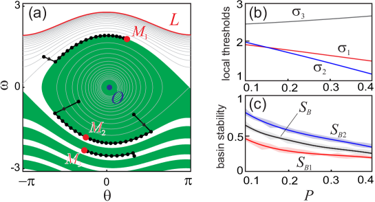
Figure 2: Stability of the pendulum (3). (a) Phase space for $\alpha=0.04$, $P=0.1.$ Green area is the attraction basin of the steady state $O$, red curve is the limit cycle $L$. LOCT points are depicted by red dots, traces of the algorithm by black. (b) Local stability thresholds $\sigma_{1}$ (red), $\sigma_{2}$ (blue), and $\sigma_{3}$ (black) versus $P$. (c) The basin stability values $S_{B1}$ (red), $S_{B2}$ (blue) and $S_{B0}$ (black) versus $P$, mean values and variances.

Next we use the concept of ST to study the attraction basin of the steady state $O$. The identified LOCT points are depicted by red dots in Fig. 2a. The most important ones are $M_{1}$ corresponding to positive perturbations and $M_{2}$ corresponding to negative ones. Because of the complex shape of the attraction basin other LOCT points exist further from the attractor, e.g. $M_{3}.$ Figure 2b demonstrates the local thresholds (LOCTs) $\sigma_{j}=\mbox{\mbox{dist}}(O,M_{j})$ associated with these points in dependence on the parameter $P.$ One can see that for $P<P^{*}\approx 0.15$ the point closest to the attractor is $M_{1},$ while for $P>P^{*}$ the closest point is $M_{2}$. Thus, the ST equals $\sigma_{1}$ for $P<P^{*}$ and $\sigma_{2}$ for $P>P^{*}$, i.e. the most dangerous are positive perturbations for small $P$ but negative perturbations for large $P$.

It is interesting to compare both basin measures: stability threshold and basin stability. For this sake $S_{B}$ is plotted versus $P$ in Fig. 2c. We calculate it for three different classes of perturbations: positive perturbations ($S_{B1}$ for $Q_{1}=[-\pi;\pi]\times[0;3]$), negative perturbations ($S_{B2}$ for $Q_{2}=[-\pi;\pi]\times[-3;0]$), and perturbations of both signs ($S_{B0}$ for $Q=Q_{1}\cup Q_{2}$). When $P$ increases, the basin stability for all classes of perturbations decreases as well as the ST. Thus, both measures indicate that the system becomes less robust. However, basin stability fails to detect which perturbations are more dangerous: $S_{B2}$ is sufficiently larger than $S_{B1}$ for all values of $P$.

We also checked that the efficiency of our algorithm is essentially improved by tracing LOCT points over the parameter. For this sake we identified the position of the point $M_{1}$ for $P\in[0.1;0.4]$ for three different setups: parameter step $\Delta P=0.02$ (16 datapoints), without tracing; the same parameter step, with tracing; smaller step $\Delta P=0.01$ (31 datapoints), with tracing. Without tracing, the search started each time from the same point. With tracing, the search for the new parameter value started from the position found for the previous parameter value. The total computation time $T_{c}$ equals $9\times 10^{-3}$(a.u.) for the first setup, $19\times 10^{-4}$ for the second setup, and $24\times 10^{-4}$ for the third setup. Thus, with tracing the computation time decreases approximately five times. For higher-dimensional systems the improvement is even much higher. Note also that $T_{c}$ in the third setup increases by less than 30% with respect to the second setup, although the number of datapoints is twice larger. The reason is that with a smaller parameter step the positions of the LOCT points change less and they are found faster.

III Stability threshold of complex networks

The second example is a network of coupled one-dimensional maps. We chose maps for two reasons: first, because of simpler implementation, and second, to demonstrate the generality of our approach. The network on $N$ nodes is governed as follows:

$$x_{i}(t+1)=ax_{i}(t)+bx_{i}^{2}(t)+\kappa\sum_{j=1}^{N}c_{ij}\left(x_{j}(t)-x_{i}(t)\right).$$ (4)

Here, $0<a<1$ is the system parameter, $\kappa$ stands for the global coupling coefficient and $c_{ij}$ are the elements of the coupling matrix. Coupling between two nodes $i$ and $j$ equals $\kappa c_{ij}$. The network has the only attractor, the stable fixed point $O(0,0,...,0)$. However, after a large perturbation the system trajectories may go to infinity.

For network (4), a natural way to find LOCT points is to trace them over the coupling coefficient $\kappa$. For $\kappa=0$, the nodes are uncoupled and each of them is governed by the map $x_{i}(t+1)=ax_{i}(t)+x_{i}^{2}(t)$, which has a stable fixed point $x_{i}=0$ with the attraction basin $-1<x_{i}<1-a$. The borders of this interval define two LOCT points in the network phase space: $M_{i+}\left(x_{j}=0\,(j\neq i),\,x_{i}=1-a\right)$ corresponds to positive perturbation of the node $i$, and $M_{i-}\left(x_{j}=0\,(j\neq i),\,x_{i}=-1\right)$ to negative ones. We start from these points for $\kappa=0$, then gradually increase $\kappa$ and trace their positions. We also periodically check for emergence of new LOCT points, but failed to detect any.

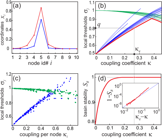
Figure 3: Stability of the network (4). (a) Coordinates of a typical LOCT point $M_{i+}$ ($i=5)$ for two values of $\kappa$ - small (blue) and large (red). (b) LOCTs $\sigma_{i\pm}$ versus $\kappa$. Blue thin curves for $\sigma_{i+}$, green thin curves for $\sigma_{i-}$. Red thick curve is the ST $\sigma$. (c) LOCTs $\sigma_{i\pm}$ versus nodal coupling strength $\kappa_{i}$ for various nodes, coupling coefficients and network configurations. Blue dots for $\sigma_{i+}$, green for $\sigma_{i-}$ (d) The basin stability versus $\kappa$. The inset shows the same dependency in logarithmic scale. Red curve for numerical results, blue thin line for the estimate (5).

We study various networks with $2\leq N\leq 100$ and different types of topology: all-to-all, random ER1960 , small-world Watts1998 , scale-free Barabasi1999 , and cluster networks Klinshov2014 . In all the cases, the behavior of LOCT points is quite similar. When $\kappa$ increases, the positions of the points change, so that the coordinates $x_{j}$ ($j\neq i$) of $M_{i\pm}$ are no longer zeros. However, for weak coupling the coordinates of LOCT points obey $|x_{i}|\gg x_{j}$, i.e. the corresponding perturbation mainly concerns the node $i$. For larger $\kappa$ the situation changes and LOCT points may have several coordinates of the same order. Typical LOCT points are illustrated in Fig. 3a.

Now let us consider LOCTs $\sigma_{i\pm}=\mbox{dist}(O,M_{i\pm})$ associated with LOCT points. A typical dependence of these thresholds on $\kappa$ is illustrated in Fig. 3b. For all $i$, $\sigma_{i+}$ grows with $\kappa$, while $\sigma_{i-}$ decreases. Some of the points $M_{i+}$ may disappear at certain $\kappa$ as well. A detailed study shows a remarkable feature of the LOCTs $\sigma_{i\pm}$: they turn out to be strongly correlated with the values of total connections strength to the node $\kappa_{i}=\kappa\sum_{j=1}^{N}c_{ij}$. In Fig. 3c the LOCTs $\sigma_{i\pm}$ are plotted versus $\kappa_{i}$ for various nodes, coupling coefficients, network sizes and configurations. The correlation is large, especially for small $\kappa_{i}$. Notice that for $\kappa_{i}\lesssim\kappa^{*}\approx 0.6$ positive perturbations have a lower threshold than negative ones, and this threshold increases with $\kappa_{i}.$ This finding leads to an easy and intuitively clear rule: the stronger the node is connected to the network the harder it is to tear it off. However, too strong coupling ($\kappa_{i}\gtrsim\kappa^{*}$) is undesirable, since it increases susceptibility to negative perturbations.

The global ST of the network is defined by the lowest LOCT. Figure 3b illustrates a typical dependence of the ST on $\kappa$.

IV Stability threshold and basin stability

It is interesting to compare the two measures of stability against large perturbations, the stability threshold and the basin stability for the same network (Fig. 3d). As the perturbation class $Q$ we use a hypersphere of radius $q=0.8$ with constant density $\rho$ which means that we consider perturbations of amplitude $q$ and random direction. Muller1959 One may see that $S_{B}=1$ when the ST exceeds $q$ for $\kappa>\kappa_{q}\approx 0.26$. This confirms that the ST indeed characterizes the weakest perturbation that can disrupt the network.

From Fig. 3d one may acquire the wrong impression that the basin stability reaches unity much earlier than $\kappa$ reaches $\kappa_{q}$. The reason is that $S_{B}$ approaches unity very quickly when $\sigma$ approaches $q$. This can be seen in the inset of Fig. 3d which has a logarithmic scale. This feature seems to be typical for high-dimensional dynamical systems. Indeed, consider an arbitrary dynamical system in the $N$-dimensional phase space settled into the attractor $\mathcal{A}$ with the stability threshold $\sigma.$ Consider the perturbation class $Q$ consisting of perturbations with the amplitude $q$. For $q<\sigma$, the set $Q$ resides inside the attraction basin $\mathcal{B}$, therefore $S_{B}=1$. For $\sigma=q$, the set $Q$ contacts the border of the basin $\delta\mathcal{B}$. For $q>\sigma$ some part of the set $Q$ gets out of the basin $\mathcal{B}$ and $S_{B}$ becomes smaller than one (Fig. 4a). The probability of the perturbed state to be out of the basin is proportional to the surface area $s$ of the protrusive part (gray in the figure), so $1-S_{B}\sim s$. To estimate the surface area, one can approximate both surfaces $Q$ and $\delta\mathcal{B}$ by quadratic forms near the site of their intersection. Then, the transverse size of the protrusive part can be estimated as $d\sim\sqrt{q-\sigma}$, and the surface area $s\sim d^{N-1}$. This leads to the estimate

$$1-S_{B}\sim(q-\sigma)^{\frac{N-1}{2}}.$$ (5)

The corresponding slope is given by the blue line in the inset of Fig. 4d and agrees with the numerical results.

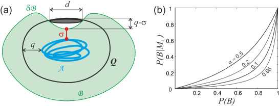
Figure 4: (a) Estimate of basin stability for perturbations slightly exceeding the ST. (b) The posterior probability $P(B|M_{1})$ versus the prior probability $P(B)$ for various values of $\alpha$ denoted on the figure.

The scaling law (5) suggests that for high-dimensional systems it is very unlikely that the system will be disrupted by a random perturbation of magnitude just above the ST. From the other side, a wisely designed perturbation can disrupt the system even being slightly above the ST.

From computational prospective, the estimate (5) shows that attempts to estimate the stability threshold from basin stability is inefficient for high-dimensional systems. Indeed, on the example from Fig. 4d one can see that it is very complicated to detect the exact point where the basin stability reaches exactly unity. The probability to randomly hit a point which is $\varepsilon$ above the stability threshold is of the order of $\varepsilon^{(N-1)/2}$, so the time to determine the threshold with the accuracy $\varepsilon$ by the brute-force strategy grows inversely. In contrast, the method suggested herein allows to reach the LOCT point and determine the ST in quite a few steps.

The estimate (5) can be also used to determine the probability of a wrong conclusion about the ST. Suppose we have a potential ST, i.e. a global minimum point $M_{1}$ with $\sigma_{1}=\mbox{dist}\left(M_{1},\mathcal{A}\right)$ and want to check if there exists another LOCT point $M_{2}$ with smaller $\sigma_{2}=\mbox{dist}\left(M_{2},\mathcal{A}\right)=\sigma_{1}-\delta\sigma$. For this sake we choose random starting points $K_{1}$ at $q=\sigma_{1}+\varepsilon$ until finding a point out of the basin and run the algorithm. If it converges to a point $M_{2}$ different from $M_{1}$ and with $\sigma_{2}<\sigma_{1}$ we have found a new potential ST. And if it converges to $M_{1}$ two competing hypotheses are to be evaluated:

Hypothesis $A$. The point $M_{1}$ indeed corresponds to the ST and there is no other point $M_{2}.$ In this case, the algorithm converges to $M_{1}$ with probability $P(M_{1}|A)=1$.

Hypothesis $B=\overline{A}$. The point $M_{2}$ exists, but we have not found it. According to (5), the probabilities to converge to $M_{1}$ and $M_{2}$ relate as

$$\frac{P(M_{1}|B)}{P(M_{2}|B)}=\alpha\sim\frac{(q-\sigma_{1})^{\frac{N-1}{2}}}{(q-\sigma_{2})^{\frac{N-1}{2}}}=\left(\frac{1}{1+\frac{\delta\sigma}{\varepsilon}}\right)^{\frac{N-1}{2}}.$$ (6)

According to Bayes’ theorem, the posterior probability $P(B|M_{1})$ is expressed through the prior probability $P(B)$ as

$$P(B|M_{1}) = \frac{P(M_{1}|B)P(B)}{P(M_{1}|A)P(A)+P(M_{1}|B)P(B)}=$$ (7)

$$= \frac{1}{1+\left(\frac{1}{\alpha}+1\right)\left(\frac{1}{P(B)}-1\right)}.$$

In Fig. 4b the posterior probability is plotted versus the prior probability for several values of $\alpha$. Note that if $\alpha$ is small enough and $P(B)$ is not close to one (7) can be approximated as $P(B|M_{1})\approx\alpha P(B)$, which means that each trial decreases the probability by the factor $\alpha$. Thus, after $M$ trials the posterior probability of $B$ can be estimated as

$$\ln P_{M}\sim-\frac{M(N-1)}{2}\ln\left(1+\frac{\delta\sigma}{\varepsilon}\right).$$ (8)

The estimate (8) gives the probability that after $M$ trials we have still missed a LOCT point whose distance to the attractor is by $\delta\sigma$ lower than $\sigma_{1}$. By sufficient increasing of $M$ this mistake probability can be made arbitrarily small.

V Conclusions and discussion

To conclude, we have introduced a novel measure to describe stability of dynamical systems against external perturbations. This is the stability threshold (ST) which equals the magnitude of the weakest perturbation capable to disrupt the established dynamical regime. The ST provides important information, since it guarantees the system to withstand any perturbation of smaller magnitude. In the phase space, the ST is the minimal distance between the system’s attractor and the border of its attraction basin. From this prospective, the ST defines the “thinnest site” of the basin. And as the saying goes, where something is thin, that is where it tears: the direction corresponding to ST is the most dangerous for the system.

For dynamical networks, different directions in the multidimensional phase space are associated with different nodes. To this end, the ST approach allows to determine the nodes which are mostly susceptible to perturbations. Applying external perturbations to these nodes, one may disrupt the network comparatively easily. However, sometimes the ST is associated with perturbations involving several nodes. An example of such a situation is depicted in Fig. 3a. Under such circumstances, it is easier to disrupt the network by simultaneous perturbation of several nodes rather than by perturbing just one of them.

We have also suggested an algorithm to calculate the ST for arbitrary dynamical systems and demonstrated its effectiveness. The generality of the ST-based approach defines its vast potential for applications. Possible fields include engineering, neuroscience, power grids, Earth science and many others where robustness of complex systems against large perturbations is important.

Besides application to the study of particular systems, further development and extension of the approach per se are of great interest. To this end, several directions are seen. The most obvious modification of the suggested approach is to apply it to problems opposite to the one considered herein. Particularly, in many applications the task is to change the behavior of the system by an external action Cornelius2013 . From the nonlinear dynamics prospective, this means pushing the system from one attractor to the basin of another. In this situation, quantification of the stability threshold immediately provides the information about the optimal perturbation to induce the switching.

Another possibility is to extend the concept of the stability threshold to multistable systems and reversible transitions between different attractors. In many applications, not a single, but several different stable regimes play essential roles, and the system may switch these regimes. The examples are switching between various patterns of activity in neural circuits Klinshov2014 ; Hopfield82 , and episodic emergence of El Niño events Ludescher13 , transitions between free flow and congestion in traffic Li15 or between failure states and active states in self-recovering networks Majdandzic13 . In all these cases, transitions in both directions are of interest. To study such transitions from one attractor to another and backwards, two stability thresholds can be introduced associated with each of the transitions. The values of these thresholds may provide important information about the transition rates when the system is externally perturbed.

Finally, the numerical algorithm can be further developed and extended for a broader class of systems. In particular, the current version of the algorithm relies on smoothness of attraction basins borders, which is a limitation of the method. It is known that basin boundaries for some dynamical systems can be fractal Grebogi83 . In this case the border can not be locally approximated by a tangential hyperplane, which is crucial to determine the direction in which to move along it. However, it is still possible to move along the border if the steps are taken in random direction. Each step is accepted if it brings the point closer to the attractor and declined otherwise. This modification of the method requires additional investigation to the define the conditions of its applicability and estimate its convergence.

References

- (1) L. M. Pecora and T. L. Carroll, Phys. Rev. Lett. 80, 2109 (1998).
- (2) H. A. Dijkstra and M. Ghil, Rev. Geophys. 43, RG3002 (2005); S. M. Rahmstorf et al, Geophys. Res. Lett. 32, L23605 (2005).
- (3) D.N. Ewart, IEEE Spectrum 15, 36 (1978).
- (4) J. Machowski, J. W. Bialek and J. R. Bumby. Power System Dynamics: Stability and Control (John Wiley & Sons, 2008).
- (5) G.A. Leonov, I.M. Burkin, and A.I. Shepeljavyi. Frequency methods in oscillation theory (Kluwer Academic Publishers, Dordrecht–Boston–London, 1996); E. Kaslik, A.M. Balint, St. Balint, Nonlinear Analysis 60, 703 (2005); N. Zhong, Proc. Am. Math. Soc. 137, 2773 (2009).
- (6) S. Jahnke, R.-M. Memmesheimer, and M. Timme, Phys. Rev. Lett. 100, 48102 (2008); R.-M. Memmesheimer, and M. Timme, Discr. Cont. Dyn. Syst 28, 1555 (2010).
- (7) D. Wiley, S.H. Strogatz, and M. Girvan, Chaos 16, 15103 (2006).
- (8) P. J. Menck, J. Heitzig, N. Marwan, and J. Kurths, Nat. Phys. 9, 89 (2013); P. J. Menck, J. Heitzig, J. Kurths, and H. J. Schellnhuber, Nat. Commun. 5, 3969 (2014).
- (9) R.G. Strongin, and Y.D. Sergeyev. Global Optimization with Non-Convex Constraints. Sequential and Parallel Algorithms. (Kluwer Academic Publishers, Dordrecht-Boston-London, 2000).
- (10) M. Rohden, A. Sorge, M. Timme and D. Witthaut, Phys. Rev. Lett. 109, 064101 (2012).
- (11) P. Erdös and A. Rényi, Publ. Math. Inst. Hung. Acad. Sci. 5, 17 (1960).
- (12) D. J. Watts and S. H. Strogatz, Nature 393, 409 (1998).
- (13) A. Barabási and R. Albert, Science 286, 509 (1999).
- (14) V.V. Klinshov, J.-n. Teramae, V.I. Nekorkin and T. Fukai, PLoS One 9, e94292 (2014).
- (15) M.E. Muller, Comm. Assoc. Comput. Mach. 2, 19 (1959).
- (16) S.P. Cornelius, W.L. Kath, and A.E. Motter, Nat. Commun. 4, 1942 (2013).
- (17) J. J. Hopfield, Proc. Natl. Acad. Sci. 79, 2554 (1982).
- (18) J. Ludescher, A. Gozolchiani, M. I. Bogachev, A. Bunde, S. Havlin, and H. J. Schellnhuber, Proc. Natl. Acad. Sci. 110, 19172 (2013).
- (19) D. Li, B. Fu, Y. Wang, G. Lu, Y. Berezin, H. E. Stanley, and S. Havlin, Proc. Natl. Acad. Sci. 112, 669 (2015).
- (20) A. Majdandzic, B. Podobnik, S. V. Buldyrev, D. Y. Kenett, S. Havlin, and H. E. Stanley, Nat. Phys. 10, 34 (2013).
- (21) C. Grebogi, E. Ott, and J. A. Yorke, Phys. Rev. Lett. 50, 935 (1983).