Feasibility Preserving Constraint-Handling Strategies for Real Parameter Evolutionary Optimization

Abstract

Evolutionary Algorithms (EAs) are being routinely applied for a variety of optimization tasks, and real-parameter optimization in the presence of constraints is one such important area. During constrained optimization EAs often create solutions that fall outside the feasible region; hence a viable constraint-handling strategy is needed. This paper focuses on the class of constraint-handling strategies that repair infeasible solutions by bringing them back into the search space and explicitly preserve feasibility of the solutions. Several existing constraint-handling strategies are studied, and two new single parameter constraint-handling methodologies based on parent-centric and inverse parabolic probability (IP) distribution are proposed. The existing and newly proposed constraint-handling methods are first studied with PSO, DE, GAs, and simulation results on four scalable test-problems under different location settings of the optimum are presented. The newly proposed constraint-handling methods exhibit robustness in terms of performance and also succeed on search spaces comprising up-to $500$ variables while locating the optimum within an error of $10^{-10}$. The working principle of the IP based methods is also demonstrated on (i) some generic constrained optimization problems, and (ii) a classic ‘Weld’ problem from structural design and mechanics. The successful performance of the proposed methods clearly exhibits their efficacy as a generic constrained-handling strategy for a wide range of applications.

Keywords constraint-handling, nonlinear and constrained optimization, particle swarm optimization, real-parameter genetic algorithms, differential evolution.

1 Introduction

Optimization problems are wide-spread in several domains of science and engineering. The usual goal is to minimize or maximize some pre-defined objective(s). Most of the real-world scenarios place certain restrictions on the variables of the problem i.e. the variables need to satisfy certain pre-defined constraints to realize an acceptable solution.

The most general form of a constrained optimization problem (with inequality constraints, equality constraints and variable bounds) can be written as a nonlinear programming (NLP) problem:

$$Minimize f(\vec{x})$$

$$Subjectto g_{j}(\vec{x})\geq 0, j=1,...,J$$ (1)

$$h_{k}(\vec{x})=0, k=1,...,K$$

$$x_{i}^{(L)}\leq x_{i}\leq x_{i}^{(U)}, i=1,...,n.$$

The NLP problem defined above contains $n$ decision variables (i.e. $\vec{x}$ is a vector of size $n$), $J$ greater-than-equal-to type inequality constraints (less-than-equal-to can be expressed in this form by multiplying both sides by $-1$), and $K$ equality-type constraints. The problem variables $x_{i}s$ are bounded by the lower ($x_{i}^{(L)}$) and upper ($x_{i}^{(U)}$) limits. When only the variable bounds are specified then the constraint-handling strategies are often termed as the boundary-handling methods.

In classical optimization, the task of constraint-handling has been addressed in a variety of ways: (i) using penalty approach developed by Fiacoo and McCormick [13], which degrades the function value in the regions outside the feasible domain, (ii) using barrier methods which operate in a similar fashion but strongly degrade the function values as the solution approaches a constraint boundary from inside the feasible space, (iii) performing search in the feasible directions using methods such gradient projection, reduced gradient and Zoutendijk’s approach [28] (iv) using the augmented Lagrangian formulation of the problem, as commonly done in linear programming and sequential quadratic programming (SQP). For a detailed account on these methods along with their implementation and convergence characteristics the reader is referred to [22, 5, 14]. The classical optimization methods reliably and effectively solve convex constrained optimization problems while ensuring convergence and therefore widely used in such scenarios. However, same is not true in the presence of non-convexity. The goal of this paper is to address the issue of constraint-handling for evolutionary algorithms in real-parameter optimization, without any limitations to convexity or a special form of constraints or objective functions.

In context to the evolutionary algorithms the constraint-handling has been addressed by a variety of methods; including borrowing of the ideas from the classical techniques. These include (i) use of penalty functions to degrade the fitness values of infeasible solutions such that the degraded solutions are given less emphasis during the evolutionary search. A common challenge in employing such penalty methods arises from choosing an appropriate penalty parameter ($R$) that strikes the right balance between the objective function value, the amount of constraint violation and the associated penalty. Usually, in EA studies, a trial-and-error method is employed to estimate $R$. A study [7] in 2000 suggested a parameter-less approach of implementing the penalty function concepts for population-based optimization method. A recent bi-objective method [4] was reported to find the appropriate $R$ values adaptively during the optimization process. Other studies [27, 26] have employed the concepts of multi-objective optimization by simultaneously considering the minimization of the constraint violation and optimization of the objective function, (ii) use of feasibility preserving operators, for example, in [15] specialized operators in the presence of linear constraints were proposed to create new and feasible-only individuals from the feasible parents. In another example, generation of feasible child solutions within the variable bounds was achieved through Simulated Binary Crossover (SBX) [6] and polynomial mutation operators [8]. The explicit feasibility of child solutions was ensured by redistributing the probability distribution function in such a manner that the infeasible regions were assigned a zero probability for child-creation [7]. Although explicit creation of feasible-only solutions during an EA search is an attractive proposition, but it may not be possible always since generic crossover or mutation operators or other standard EAs do not gaurantee creation of feasible-only solutions, (iii) deployment of repair strategies that bring an infeasible solution back into the feasible domain. Recent studies [19, 11, 10, 3] investigated the issue of constraint-handling through repair techniques in context to PSO and DE, and showed that the repair mechanisms can introduce a bias in the search and hinder exploration. Several repair methods proposed in context PSO [16, 12, 1] exploit the information about location of the optimum and fail to perform when the location of optimum changes [17]. These issues are universal and often encountered with all EAs (as shown in later sections). Furthermore, the choice of the evolutionary optimizer, the constraint-handling strategy, and the location of the optima with respect to the search space, all play an important role in the optimization task. To this end, authors have realized a need for a reliable and effective repair-strategy that explicitly preserves feasibility. An ideal evolutionary optimizer (evolutionary algorithm and its constrained-handling strategy) should be robust in terms of finding the optimum, irrespective of the location of the optimal location in the search space. In rest of the paper, the term constraint-handling strategy refers to explicit feasibility preserving repair techniques.

First we review the existing constraint-handling strategies and then propose two new constraint-handling schemes, namely, Inverse Parabolic Methods (IPMs). Several existing and newly proposed constrained-handling strategies are first tested on a class of benchmark unimodal problems with variable bound constraints. Studying the performance of constraint-handling strategies on problems with variable bounds allows us to gain better understanding into the operating principles in a simplistic manner. Particle Swarm Optimization, Differential Evolution and real-coded Genetic Algorithms are chosen as evolutionary optimizers to study the performance of different constraint-handling strategies. By choosing different evolutionary optimizers, better understanding on the functioning of constraint-handlers embedded in the evolutionary frame-work can be gained. Both, the search algorithm and constraint-handling strategy must operate efficiently and synergistically in order to successfully carry out the optimization task. It is shown that the constraint-handling methods possessing inherent pre-disposition; in terms of bringing infeasible solutions back into the specific regions of the feasible domain, perform poorly. Deterministic constraint-handling strategies such as those setting the solutions on the constraint boundaries result in the loss of population diversity. On the other hand, random methods of bringing the solutions back into the search space arbitrarily; lead to complete loss of all useful information carried by the solutions. A balanced approach that utilizes the useful information from the solutions and brings them back into the search space in a meaningful way is desired. The newly proposed IPMs are motivated by these considerations. The stochastic and adaptive components of IPMs (utilizing the information of the solution’s feasible and infeasible locations), and a user-defined parameter ($\alpha$) render them quite effective.

The rest of the paper is organized as follows: Section 2 reviews existing constraint-handling techniques commonly employed for problems with variable bounds. Section 3 provides a detailed description on two newly proposed IPMs. Section 4 provides a description on the benchmark test problems and several simulations performed on PSO, GAs and DE with different constraint-handling techniques. Section 5 considers optimization problems with larger number of variables. Section 6 shows the extension and applicability of proposed IPMs for generic constrained problems. Finally, conclusions and scope for future work are discussed in Section 7.

2 Feasibility Preserving Constraint-Handling Approaches for Optimization Problems with Variable Bounds

Several constraint-handling strategies have been proposed to bring solutions back into the feasible region when constraints manifest as variable bounds. Some of these strategies can also be extended in presence of general constraints. An exhaustive recollection and comparison of all the constraint-handling techniques is beyond the scope of this study. Rather, we focus our discussions on the popular and representative constraint-handling techniques.

The existing constraint-handling methods for problems with variable bounds can be broadly categorized into two groups: Group $A$ techniques that perform feasibility check variable wise, and Group $B$ techniques that perform feasibility check vector-wise. According to Group $A$ techniques, for every solution, each variable is tested for its feasibility with respect to its supplied bounds and made feasible if the corresponding bound is violated. Here, only the variables violating their corresponding bounds are altered, independently, and other variables are kept unchanged. According to Group $B$ techniques, if a solution (represented as a vector) is found to violate any of the variable bounds, it is brought back into the search space along a vector direction into the feasible space. In such cases, the variables that explicitly do not violate their own bounds may also get modified.

It is speculated that for variable-wise separable problems, that is, problems where variables are not linked to one another, techniques belonging to Group $A$ are likely to perform well. However, for the problems with high correlation amongst the variables (usually referred to as linked-problems), Group $B$ techniques are likely to be more useful. Next, we provide description of these constraint-handling methods in detail .

2.1 Random Approach

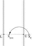
Figure 1: Variable-wise random approach for handling bounds.

This is one of the simplest and commonly used approaches for handling boundary violations in EAs [3]. This approach belongs to Group $A$. Each variable is checked for a boundary violation and if the variable bound is violated by the current position, say $x_{i}^{c}$, then $x_{i}^{c}$ is replaced with a randomly chosen value $y_{i}$ in the range $[x_{i}^{(L)},x_{i}^{(U)}]$, as follows:

$$y_{i}=\mbox{random}[x_{i}^{(L)},x_{i}^{(U)}].$$ (2)

Figure 1 illustrates this approach. Due to the random choice of the feasible location, this approach explicitly maintains diversity in the EA population.

2.2 Periodic Approach

Figure 2: Variable-wise periodic approach for handling bounds.

This strategy assumes a periodic repetition of the objective function and constraints with a period $p=x_{i}^{(U)}-x_{i}^{(L)}$. This is carried out by mapping a violated variable $x_{i}^{c}$ in the range $[x_{i}^{(L)},x_{i}^{(U)}]$ to $y_{i}$, as follows:

$$y_{i}=\left\{\begin{array}[]{ll}x_{i}^{(U)}-(x_{i}^{(L)}-x_{i}^{c})\%p,&\quad\text{if $x_{i}^{c}<x_{i}^{(L)}$},\\ x_{i}^{(L)}+(x_{i}^{c}-x_{i}^{(U)})\%p,&\quad\text{if $x_{i}^{c}>x_{i}^{(U)}$},\\ \end{array}\right.$$ (3)

In the above equation, % refers to the modulo operator. Figure 2 describes the periodic approach. The above operation brings back an infeasible solution in a structured manner to the feasible region. In contrast to the random method, the periodic approach is too methodical and it is unclear whether such a repair mechanism is supportive of preserving any meaningful information of the solutions that have created the infeasible solution. This approach belongs to Group $A$.

2.3 SetOnBoundary Approach

As the name suggests, according to this strategy a violated variable is reset on the bound of the variable which it violates.

$$y_{i}=\left\{\begin{array}[]{ll}x_{i}^{(L)},&\quad\text{if $x_{i}^{c}<x_{i}^{(L)}$},\\ x_{i}^{(U)},&\quad\text{if $x_{i}^{c}>x_{i}^{(U)}$}.\\ \end{array}\right.$$ (4)

Clearly this approach forces all violated solutions to lie on the lower or on the upper boundaries, as the case may be. Intuitively, this approach will work well on the problems when the optimum of the problem lies exactly on one of the variable boundaries. This approach belongs to Group $A$.

2.4 Exponentially Confined (Exp-C) Approach

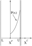
Figure 3: Variable-wise exponentially approach (Exp-C) for handling bounds.

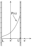
Figure 4: Variable-wise exponentially approach (Exp-S) for handling bounds.

This method was proposed in [1]. According to this approach, a particle is brought back inside the feasible search space variable-wise in the region between its old position and the violated bound. The new location is created in such a manner that higher sampling probabilities are assigned to the regions near the violated boundary. The developers suggested the use of an exponential probability distribution, shown in Figure 4. The motivation of this approach is based on the hypothesis that a newly created infeasible point violates a particular variable boundary because the optimum solution lies closer to that variable boundary. Thus, this method will probabilistically create more solutions closer to the boundaries, unless the optimum lies well inside the restricted search space. This approach belongs to Group $A$.

Assuming that the exponential distribution is $p(x_{i})=A\exp(|x_{i}-x_{i}^{p}|)$, the value of $A$ can be obtained by integrating the probability from $x_{i}=x_{i}^{p}$ to $x_{i}=x_{i}^{(B)}$ (where $B=L$ or $U$, as the case may be). Thus, the probability distribution is given as $p(x)=\exp(|x_{i}-x_{i}^{p}|)/(\exp(|x_{i}^{(B)}-x_{i}^{p}|)-1)$. For any random number $r$ within $[0,1]$, the feasible solution is calculated as follows:

$$y_{i}=\left\{\begin{array}[]{ll}x_{i}^{p}-\ln(1+r(\exp(x_{i}^{p}-x_{i}^{(L)})-1))&\mbox{if $x_{i}<x_{i}^{(L)}$},\\ x_{i}^{p}+\ln(1+r(\exp(x_{i}^{(U)}-x_{i}^{p})-1)),&\mbox{if $x_{i}>x_{i}^{(U)}$}.\end{array}\right.$$ (5)

2.5 Exponential Spread (Exp-S) Approach

This is a variation of the above approach, in which, instead of confining the probability to lie between $x_{i}^{p}$ and the violated boundary, the exponential probability is spread over the entire feasible region, that is, the probability is distributed from lower boundary to the upper boundary with an increasing probability towards the violated boundary. This requires replacing $x_{i}^{p}$ with $x_{i}^{(U)}$ (when the lower boundary is violated) or $x_{i}^{(L)}$ (when the upper boundary is violated) in the Equation 5 as follows:

$$y_{i}=\left\{\begin{array}[]{ll}x_{i}^{(U)}-\ln(1+r(\exp(x_{i}^{(U)}-x_{i}^{(L)})-1))&\mbox{if $x_{i}<x_{i}^{(L)}$},\\ x_{i}^{(L)}+\ln(1+r(\exp(x_{i}^{(U)}-x_{i}^{(L)})-1)),&\mbox{if $x_{i}>x_{i}^{(U)}$}.\end{array}\right.$$ (6)

The probability distribution is shown in Figure 4. This approach also belongs to Group $A$.

2.6 Shrink Approach

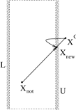
Figure 5: Vector based SHR. strategy for handling bounds.

This is a vector-wise approach and belongs to Group $B$ in which the violated solution is set on the intersection point of the line joining the parent point ($\vec{x}_{not}$), child point ($\vec{x}^{c})$, and the violated boundary. Mathematically, the mapped vector $\vec{y}$ is created as follows:

$$\vec{y}=\vec{x}_{not}+\beta(\vec{x}^{c}-\vec{x}_{not}),$$ (7)

where $\beta$ is computed as the minimum of all positive values of intercept $(x_{i}^{(L)}-x_{i,not})/(x_{i}^{c}-x_{i,not})$ for a violated boundary $x_{i}^{(L)}$ and $(x_{i}^{(U)}-x_{i,not})/(x_{i}^{c}-x_{i,not})$ for a violated boundary $x_{i}^{(U)}$. This operation is shown in Figure 5. In the case shown, $\beta$ needs to be computed for variable bound $x_{2}^{(U)}$ only.

3 Proposed Inverse Parabolic (IP) Constraint-Handling Methods

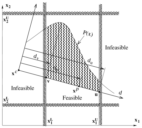
Figure 6: Vector based Inverse Parabolic Methods.

The exponential probability distribution function described in the previous section brings violated solutions back into the allowed range variable-wise, but ignores the distance of the violated solution $x_{i}^{c}$ with respect to the violated boundary. The distance from the violated boundary carries useful information for remapping the violated solution into the feasible region. One way to utilize this distance information is to bring solutions back into the allowed range with a higher probability closer to the boundary, when the fallen-out distance ($d_{v}$, as shown in Figure 6) is small. In situations, when points are too far outside the allowable range, that is, the fallen-out distance $d_{v}$ is large, particles are brought back more uniformly inside the feasible range. Importantly, when the fallen-out distance $d_{v}$ is small (meaning that the violated child solution is close to the variable boundary), the repaired point is also close to the violated boundary but in the feasible side. Therefore, the nature of the exponential distribution should become more and more like a uniform distribution as the fallen-out distance $d_{v}$ becomes large.

Let us consider Figure 6 which shows a violated solution $\vec{x}^{c}$ and its parent solution $\vec{x}^{p}$. Let $d_{p}=\|\vec{x}^{c}-\vec{x}^{p}\|$ denote the distance between the violated solution and the parent solution. Let $\vec{v}$ and $\vec{u}$ be the intersection points of the line joining $\vec{x}^{c}$ and $\vec{x}^{p}$ with the violated boundary and the non-violated boundary, respectively. The corresponding distances of these two points from $\vec{x}^{c}$ are $d_{v}$ and $d_{u}$, respectively. Clearly, the violated distance is $d_{v}=\|\vec{x}^{c}-\vec{v}\|$. We now define an inverse parabolic probability distribution function from $\vec{x}^{c}$ along the direction $(\vec{x}^{p}-\vec{x}^{c})$ as:

$$p(d)=\frac{A}{(d-d_{v})^{2}+\alpha^{2}d_{v}^{2}},\quad d_{v}\leq d\leq a,$$ (8)

where $a$ is the upper bound of $d$ allowed by the constraint-handling scheme (we define $a$ later) and $\alpha$ is a pre-defined parameter. By calculating and equating the cumulative probability equal to one, we find:

$$A=\frac{\alpha d_{v}}{\tan^{-1}\frac{a-d_{v}}{\alpha d_{v}}}.$$

The probability is maximum at $d=d_{v}$ (at the violated boundary) and reduces as the solution enters the allowable range. Although this characteristic was also present in the exponential distribution, the above probability distribution is also a function of violated distance $d_{v}$, which acts like a variance to the probability distribution. If $d_{v}$ is small, then the variance of the distribution is small, thereby resulting in a localized effect of creating a mapped solution. For a random number $r\in[0,1]$, the distance of the mapped solution from $\vec{x}^{c}$ in the allowable range $[d_{v},d_{u}]$ is given as follows:

$$d^{\prime}=d_{v}+\alpha d_{v}\tan\left(r\tan^{-1}\frac{a-d_{v}}{\alpha d_{v}}\right).$$ (9)

The corresponding mapped solution is as follows:

$$\vec{y}=\vec{x}^{c}+d^{\prime}(\vec{x}^{p}-\vec{x}^{c}).$$ (10)

Note that the IP method makes a vector-wise operation and is sensitive to the relative locations of the infeasible solution, the parent solution, and the violated boundary.

The parameter $\alpha$ has a direct external effect of inducing small or large variance to the above probability distribution. If $\alpha$ is large, the variance is large, thereby having uniform-like distribution. Later we shall study the effect of the parameter $\alpha$. A value $\alpha$ $\approx$ 1.2 is found to work well in most of the problems and is recommended. Next, we describe two particular constraint-handling schemes employing this probability distribution.

3.1 Inverse Parabolic Confined (IP-C) Method

In this approach, the probability distribution is confined between $d\in[d_{v},d_{p}]$, thereby making $a=d_{p}$. Here, a mapped solution $\vec{y}$ lies strictly between violated boundary location ($\vec{v}$) and the parent ($\vec{x}^{p}$).

3.2 Inverse Parabolic Spread (IP-S) Method

Here, the mapped solution is allowed to lie in the entire feasible range between $\vec{v}$ and $\vec{u}$ along the vector $(\vec{x}^{p}-\vec{x}^{c})$, but more emphasis is given on relocating the child near the violated boundary. The solution can be found by using Equations 9 and 10, and by setting $a=d_{u}$.

4 Results and Discussions

In this study, first we choose four standard scalable unimodal test functions (in presence of variable bounds): Ellipsoidal ($F_{\rm elp}$), Schwefel ($F_{\rm sch}$), Ackley ($F_{\rm sch}$), and Rosenbrock ($F_{\rm ros}$), described as follows:

$$F_{\rm elp} = \sum_{i=1}^{n}ix_{i}^{2}$$ (11)

$$F_{\rm sch} = \sum_{i=1}^{n}\left(\sum_{j=1}^{i}x_{j}\right)^{2}$$ (12)

$$F_{\rm ack} = -20exp\left(-0.2\sqrt{\frac{1}{n}\sum_{i=1}^{i=n}x_{i}^{2}}\right)-exp\left(\frac{1}{n}\sum_{i=1}^{n}cos(2\pi x_{i})\right)+20+e$$ (13)

$$F_{\rm ros} = \sum_{i=1}^{n-1}(100(x_{i}^{2}-x_{i+1})^{2}+(x_{i}-1)^{2})$$ (14)

In the unconstrained space, $F_{\rm elp}$, $F_{\rm sch}$ and $F_{\rm ack}$ have a minimum at $x_{i}^{\ast}=0$, whereas $F_{ros}$ has a minimum at $x_{i}^{\ast}=1$. All functions have minimum value $F^{\ast}=0$. $F_{\rm elp}$ is the only variable separable problem. $F_{\rm ros}$ is a challenging test problem that has a ridge which poses difficulty for several optimizers. In all the cases the number of variables is chosen to be $n=20$.

For each test problem three different scenarios corresponding to the relative location of the optimum with respect to the allowable search range are considered. This is done by selecting different variable bounds, as follows:

On the Boundary:

Optimum is exactly on one of the variable boundaries (for $F_{\rm elp}$, $F_{\rm sch}$ and $F_{\rm ack}$ $x_{i}\in[0,10]$, and for $F_{\rm ros}$, $x_{i}\in[1,10]$),

At the Center:

Optimum is at the center of the allowable range (for $F_{\rm elp}$, $F_{\rm sch}$ and $F_{\rm ack}$ $x_{i}\in[-10,10]$, and for $F_{\rm ros}$, $x_{i}\in[-8,10]$), and

Close to Boundary:

Optimum is near the variable boundary, but not exactly on the boundary (for $F_{\rm elp}$, $F_{\rm sch}$ and $F_{\rm ack}$ $x_{i}\in[-1,10]$, and for $F_{\rm ros}$, $x_{i}\in[0,10]$).

These three scenarios are shown in the Figure 7 for a two-variable problem having variable bounds: $x_{i}^{(L)}=0$ and $x_{i}^{(U)}=10$. Although in practice, the optimum can lie anywhere in the allowable range, the above three scenarios pose adequate representation of different possibilities that may exist in practice.

Figure 7: Location of optimum for $F_{elp}$: (a) on the boundary (b) in the center and (c) close to the edge of the boundary by selecting different search domains.

For each test problem, the population is initialized uniformly in the allowable range. We count the number of function evaluations needed for the algorithm to find a solution close to the known optimum solution and we call this our evaluation criterion $S$. Choosing a high accuracy (i.e. small value of $S$) as the termination criteria minimizes the chances of locating the optimum due to random effects, and provides a better insight into the behavior of a constraint-handling mechanism.

To eliminate the random effects and gather results of statistical importance, each algorithm is tested on a problem $50$ times (each run starting with a different initial population). A particular run is terminated if the evaluation criterion $S$ is met (noted as a successful run), or the number of function evaluations exceeds one million (noted as an unsuccessful run). If only a few out of the $50$ runs are successful, then we report the number of successful runs in the bracket. In this case, the best, median and worst number of function evaluations are computed from the successful runs only. If none of the runs are successful, we denote this by marking (DNC) (Did Not Converge). In such cases, we report the best, median and worst attained function values of the best solution at the end of each run. To distinguish the unsuccessful results from successful ones, we present the fitness value information of the unsuccessful runs in italics.

An in-depth study on the constraint-handling techniques is carried out in this paper. Different locations of the optimum are selected and systematic comparisons are carried out for PSO, DE and GAs in Sections  4.1,  4.3 and  4.4 , respectively.

4.1 Results with Particle Swarm Optimization (PSO)

In PSO, decision variable and the velocity terms are updated independently. Let us say, that the initial position is $\vec{x}_{t}$, the newly created position is infeasible and represented by $\vec{x}_{t+1}$, and the repaired solution is denoted by $\vec{y}_{t}$.

If the velocity update is based on the infeasible solution as:

$$\vec{v}_{t+1}=\vec{x}_{t+1}-\vec{x}_{t}$$ (15)

then, we refer to this as “Velocity Unchanged”. However, if the velocity update is based on the repaired location as:

$$\vec{v}_{t+1}=\vec{y}_{t}-\vec{x}_{t},$$ (16)

then, we refer to this as “Velocity Recomputed”. This terminology is used for rest of the paper. For inverse parabolic (IP) and exponential (Exp) approaches, we use “Velocity Recomputed” strategy only. We have performed “Velocity Unchanged” strategy with IP and exponential approaches, but the results were not as good as compared to “Velocity Recomputed” strategy. For the SetOnBoundary approach, we use the “Velocity Recomputed” strategy and two other strategies discussed as follows.

Another strategy named “Velocity Reflection” is used, which simply implies that if a particle is set on the $i$-th boundary, then $v_{i}^{t+1}$ is changed to $-v_{i}^{t+1}$. The goal of the velocity reflection is to explicitly allow particles to move back into the search space. In the “Velocity Set to Zero” strategy, if a particle is set on the $i$-th boundary, then the corresponding velocity component is set to zero i.e. $v_{i}^{t+1}=0$. For the shrink approach, both “Velocity Recomputed” and “Velocity Set to Zero” strategies are used.

For PSO, a recently proposed hyperbolic [11] constraint-handling approach is also included in this study. This strategy operates by first calculating velocity according to the standard mechanism  15, and in the case of violation a linear normalization is performed on the velocity to restrict the solution from jumping out of the constrained boundary as follows:

$$v_{i,t+1}=\frac{v_{i,t+1}}{1+\frac{|v_{i,t+1}|}{\min(x_{i}^{(U)}-x_{i},x_{i,t}-x_{i}^{(L)})}}.$$ (17)

Essentially, the closer the particle gets to the boundary (e.g., $x_{i,t}$ only slightly smaller than $x_{i}^{(U)}$), the more difficult it becomes to reach the boundary. In fact, the particle is never completely allowed to reach the boundary as the velocity tends to zero. We emphasize again that this strategy is only applicable to PSO. A standard PSO is employed in this study with a population size of 100. The results for all the above scenarios with PSO are presented in Tables 1 to  4.

Table 1: Results on $F_{\rm elp}$ with PSO for $10^{-10}$ termination criterion.

Strategy	Velocity update	Best	Median	Worst
$F_{\rm elp}$ in [0,10]: On the Boundary
IP Spread	Recomputed	39,900	47,000	67,000
IP Confined	Recomputed	47,900 (49)	88,600	140,800
Exp. Spread	Recomputed	3.25e-01	5.02e-01	1.08e+00
Exp. Confined	Recomputed	4,600	5,900	7,500
Periodic	Recomputed	3.94e+02 (DNC)	6.63e+02	1.17e+03
Periodic	Unchanged	8.91e+02 (DNC)	1.03e+03	1.34e+03
Random	Recomputed	1.97e+01 (DNC)	3.37e+01	8.10e+01
Random	Unchanged	5.48e+02 (DNC)	6.69e+02	9.65e+02
SetOnBoundary	Recomputed	900 (44)	1,300	5,100
SetOnBoundary	Reflected	242,100	387,100	811,400
SetOnBoundary	Set to Zero	1,300 (48)	1,900	4,100
Shrink	Recomputed	8,200 (49)	10,900	14,300
Shrink	Set to Zero	33,000	40,700	53,900
Hyperbolic	Modified (Eq. (17))	14,100	15,100	16,500
$F_{\rm elp}$ in [-10,10]: At the Center
IP Spread	Recomputed	31,600	34,000	37,900
IP Confined	Recomputed	30,900	33,800	38,500
Exp. Spread	Recomputed	30,500	34,700	38,300
Exp. Confined	Recomputed	31,900	35,100	38,200
Periodic	Recomputed	32,200	35,100	37,900
Periodic	Unchanged	33,800	36,600	41,200
Random	Recomputed	31,900	34,800	37,400
Random	Unchanged	31,600	34,900	38,100
SetOnBoundary	Recomputed	31,900	35,500	40,500
SetOnBoundary	Reflected	50,800 (38)	83,200	484,100
SetOnBoundary	Set to Zero	31,600	35,000	37,200
Shrink	Recomputed	32,000	34,400	48,200
Shrink	Set to Zero	31,400	34,000	37,700
Hyperbolic	Modified (Eq. (17))	29,400	31,200	34,700
$F_{\rm elp}$ in [-1,10]: Close to Boundary
IP Spread	Recomputed	28,200	31,900	35,300
IP Confined	Recomputed	28,300	32,900	44,600
Exp. Spread	Recomputed	28,300	30,700	33,200
Exp. Confined	Recomputed	29,500	33,000	44,700
Periodic	Recomputed	4.86e+01 (DNC)	1.41e+02	4.28e+02
Periodic	Unchanged	2.84e+02 (DNC)	5.46e+02	8.28e+02
Random	Recomputed	36,900	41,900	45,600
Random	Unchanged	1.13e+02 (DNC)	2.26e+02	4.35e+02
SetOnBoundary	Recomputed	1.80e+01 (DNC)	7.60e+01	3.00e+02
SetOnBoundary	Reflected	2.13e-01 (DNC)	2.17e+01	1.06e+02
SetOnBoundary	Set to Zero	31,700 (2)	31,700	32,600
Shrink	Recomputed	29,500 (6)	36,100	42,300
Shrink	Set to Zero	28,400 (36)	32,700	65,600
Hyperbolic	Modified (Eq. (17))	25,900	29,200	31,000

Table 2: Results on $F_{\rm sch}$ with PSO for $10^{-10}$ termination criterion.

Strategy	Velocity	Best	Median	Worst
$F_{\rm sch}$ in [0,10]: On the Boundary
IP Spread	Recomputed	67,200	257,800	970,400
IP Confined	Recomputed	112,400 (6)	126,500	145,900
Exp. Spread	Recomputed	3.79e+00 (DNC)	8.37e+00	1.49e+01
Exp. Confined	Recomputed	4,900	6,100	13,500
Periodic	Recomputed	4.85e+03 (DNC)	7.82e+03	1.34e+04
Periodic	Unchanged	7.69e+03 (DNC)	1.11e+04	1.51e+04
Random	Recomputed	2.61e+02 (DNC)	5.44e+02	1.05e+03
Random	Unchanged	5.30e+03 (DNC)	7.60e+03	1.22e+04
SetOnBoundary	Recomputed	800 (30)	1,100	3,900
SetOnBoundary	Reflected	171,500	241,700	434,200
SetOnBoundary	Set to Zero	1,000 (40)	1,600	5,300
Shrink	Recomputed	6,900	9,100	11,600
Shrink	Set to Zero	17,900	31,900	49,800
Hyperbolic	Modified (Eq. (17))	36,400	41,700	48,700
$F_{\rm sch}$ in [-10,10]: At the Center
IP Spread	Recomputed	106,700	127,500	144,300
IP Confined	Recomputed	111,500	130,100	149,900
Exp. Spread	Recomputed	112,300	131,400	149,000
Exp. Confined	Recomputed	116,400	131,300	148,200
Periodic	Recomputed	113,400	130,900	150,600
Periodic	Unchanged	121,200	137,800	159,100
Random	Recomputed	112,900	129,800	151,100
Random	Unchanged	117,000	130,600	148,100
SetOnBoundary	Recomputed	118,500 (49)	132,300	161,100
SetOnBoundary	Reflected	3.30e-06 (DNC)	8.32e+01(DNC)	2.95e+02 (DNC)
SetOnBoundary	Set to Zero	111,900	132,200	149,700
Shrink.	Recomputed	111,800 (49)	131,800	183,500
Shrink.	Set to Zero	108,400	125,100	143,600
Hyperbolic	Modified (Eq. (17))	101,300	117,700	129,700
$F_{\rm sch}$ in [-1,10]: Close to Boundary
IP Spread	Recomputed	107,200	130,400	272,400
IP Confined	Recomputed	120,100 (44)	171,200	301,200
Exp. Spread	Recomputed	92,800	109,200	126,400
Exp. Confined	Recomputed	110,200	127,400	256,100
Periodic	Recomputed	8.09e+02 (DNC)	2.01e+03 (DNC)	5.53e+03(DNC)
Periodic	Unchanged	2.16e+03 (DNC)	4.36e+03 (DNC)	6.87e+03 (DNC)
Random	Recomputed	123,300	165,600	280,000
Random	Unchanged	8.17e+02 (DNC)	1.96e+03 (DNC)	2.68e+03 (DNC)
SetOnBoundary	Recomputed	2.50e+00 (DNC)	1.25e+01 (DNC)	5.75e+02 (DNC)
SetOnBoundary	Reflected	1.86e+00 (DNC)	7.76e+00 (DNC)	5.18e+01 (DNC)
SetOnBoundary	Set to Zero	1.00e+00 (DNC)	5.00e+00 (DNC)	4.21e+02 (DNC)
Shrink	Recomputed	5.00e-01 (DNC)	3.00e+00 (DNC)	1.60e+01 (DNC)
Shrink	Set to Zero	108,300 (8)	130,300	143,000
Hyperbolic	Modified (Eq. (17))	93,100	108,300	119,000

Table 3: Results on $F_{\rm ack}$ with PSO for $10^{-10}$ termination criterion.

Strategy	Best	Median	Worst
$F_{\rm ack}$ in [0,10]: On the Boundary
IP Spread	Recomputed	150,600 (49)	220,900	328,000
IP Confined	Recomputed	4.17e+00 (DNC)	6.53e+00	8.79e+00
Exp. Spread	Recomputed	2.76e-01 (DNC)	9.62e-01	2.50e+00
Exp. Confined	Recomputed	7,800	9,600	11,100
Periodic	Recomputed	6.17e+00 (DNC)	6.89e+00	9.22e+00
Periodic	Unchanged	8.23e+00 (DNC)	9.10e+00	9.68e+00
Random	Recomputed	3.29e+00 (DNC)	3.40e+00	4.19e+00
Random	Unchanged	6.70e+00 (DNC)	7.46e+00	8.57e+00
SetOnBoundary	Recomputed	800	1,100	2,100
SetOnBoundary	Reflected	420,600	598,600	917,400
SetOnBoundary	Set to Zero	1,100	1,800	3,100
Shrink.	Recomputed	33,800 (5)	263,100	690,400
Shrink.	Set Zero	3.65e+00 (DNC)	6.28e+00	8.35e+00
Hyperbolic	Modified (Eq. (17))	24,600 (25)	26,100	28,000
$F_{\rm ack}$ in [-10,10]: At the Center
IP Spread	Recomputed	53,900 (46)	58,600	66,500
IP Confined	Recomputed	54,800 (49)	59,200	64,700
Exp. Spread	Recomputed	55,100	59,300	63,600
Exp. Confined	Recomputed	56,800	59,600	65,000
Periodic	Recomputed	55,700 (48)	59,900	64,700
Periodic	Unchanged	57,900 (49)	62,100	66,700
Random	Recomputed	55,100 (47)	59,400	65,100
Random	Unchanged	56,300	59,700	65,500
SetOnBoundary	Recomputed	55,100 (49)	58,900	65,400
SetOnBoundary	Reflected	86,900 (4)	136,400	927,600
SetOnBoundary	Set to Zero	53,900 (49)	59,600	67,700
Shrink	Recomputed	55,800 (47)	58,700	65,800
Shrink	Set to Zero	55,700 (49)	58,900	62,000
Hyperbolic	Modified (Eq. (17))	52,900 (49)	56,200	64,400
$F_{\rm ack}$ in [-1,10]: Close to Boundary
IP Spread	Recomputed	54,600 (5)	55,100	56,600
IP Confined	Recomputed	63,200 (1)	63,200	63,200
Exp. Spread	Recomputed	51,300	55,200	58,600
Exp. Confined	Recomputed	1.42e+00 (DNC)	2.17e+00	2.92e+00
Periodic	Recomputed	2.88e+00 (DNC)	4.03e+00	5.40e+00
Periodic	Unchanged	6.61e+00 (DNC)	7.46e+00	8.37e+00
Random	Recomputed	60,300 (45)	66,200	72,200
Random	Unchanged	4.21e+00 (DNC)	4.93e+00	6.11e+00
SetOnBoundary	Recomputed	2.74e+00 (DNC)	3.16e+00	3.36e+00
SetOnBoundary	Reflected	824,700 (1)	824,700	824,700
SetOnBoundary	Set to Zero	1.70e+00 (DNC)	2.63e+00	3.26e+00
Shrink	Recomputed	1.45e+00 (DNC)	2.34e+00	2.73e+00
Shrink	Set to Zero	2.01e+00 (DNC)	3.96e+00	6.76e+00
Hyperbolic	Modified (Eq. (17))	50,000 (39)	53,500	58,100

Table 4: Results on $F_{\rm ros}$ with PSO for $10^{-10}$ termination criterion.

Strategy	Best	Median	Worst
$F_{\rm ros}$ in [1,10]: On the Boundary
IP Spread	Recomputed	89,800	195,900	243,300
IP Confined	Recomputed	23,800	164,300	209,300
Exp. Spread	Recomputed	9.55e-01 (DNC)	2.58e+00	7.64e+00
Exp. Confined	Recomputed	3,700	128,100	344,400
Periodic	Recomputed	1.24e+04 (DNC)	2.35e+04	4.24e+04
Periodic	Unchanged	6.99e+04 (DNC)	1.01e+05	1.45e+05
Random	Recomputed	6.00e+01 (DNC)	1.37e+02	4.42e+02
Random	Unchanged	2.32e+04 (DNC)	3.90e+04	8.22e+04
SetOnBoundary	Recomputed	900 (45)	1,600	89,800
SetOnBoundary	Reflected	2.14e-03 (DNC)	6.01e+02	5.10e+04
SetOnBoundary	Set to Zero	1,400 (48)	3,000	303,700
Shrink.	Recomputed	3,900 (44)	5,100	406,000
Shrink.	Set to Zero	15,500	136,200	193400
Hyperbolic		177,400 (45)	714,300	987,500
$F_{\rm ros}$ in [-8,10]: Near the Center
IP Spread	Recomputed	302,300 (28)	774,900	995,000
IP Confined	Recomputed	296,600 (32)	729,000	955,000
Exp. Spread	Recomputed	208,800 (24)	754,700	985,200
Exp. Confined	Recomputed	301,100 (33)	801,400	961,800
Periodic	Recomputed	26,200 (27)	705,100	986,200
Periodic	Unchanged	247,300 (32)	776,800	994,900
Random	Recomputed	311,200 (30)	809,300	990,800
Random	Unchanged	380,100 (29)	793,300	968,300
SetOnBoundary	Recomputed	248,700 (35)	795,600	973,900
SetOnBoundary	Reflected	661,900 (01)	661,900	661,900
SetOnBoundary	Set to Zero	117,400 (25)	858,400	995,400
Shrink.	Recomputed	347,900 (33)	790,500	996,300
Shrink.	Set to Zero	353,300 (26)	788,700	986,800
Hyperbolic	Modified (Eq. (17))	6.47e-08 (DNC)	1.27e-04 (DNC)	6.78e+00 (DNC)
$F_{\rm ros}$ in [1,10]: Close to Boundary
IP Spread	Recomputed	184,600 (47)	442,200	767,500
IP Confined	Recomputed	229,900 (40)	457,600	899,200
Exp. Spread	Recomputed	19,400 (47)	378,200	537,300
Exp. Confined	Recomputed	6.79e-03 (DNC)	4.23e+00	6.73e+01
Periodic	Recomputed	1.51e-02 (DNC)	3.73e+00	5.17e+02
Periodic	Unchanged	1.92e+04 (DNC)	2.86e+04	6.71e+04
Random	Recomputed	103,800	432,200	527,200
Random	Unchanged	2.33e+02 (DNC)	1.47e+03	4.23e+03
SetOnBoundary	Recomputed	1.71e+01 (DNC)	1.87e+01	3.13e+02
SetOnBoundary	Reflected	6.88e+00 (DNC)	5.52e+02	2.14e+04
SetOnBoundary	Set to Zero	6.23e+00 (DNC)	1.80e+01	3.12e+02
Shrink	Recomputed	350,300 (3)	350,900	458,400
Shrink	Set to Zero	163,700 (26)	418,000	531,900
Hyperbolic	Modified (Eq. (17))	920,900 (1)	920,900	920,900

The extensive simulation results are summarized using the following method. For each (say $j$) of the 14 approaches, the corresponding number of the successful applications ($\rho_{j}$) are recorded. Here, an application is considered to be successful if more than 45 runs out of 50 runs are able to find the optimum within the specified accuracy. It is observed that IP-S is successful in 10 out of 12 problem instances. Exponential confined approach (Exp-C) is successful in 9 cases. To investigate the required number of function evaluations (FE) needed to find the optimum, by an approach (say $j$), we compute the average number of $\bar{\rm FE}_{k}^{j}$ needed to solve a particular problem ($k$) and construct the following objective for $j$-th approach:

$$\mbox{FE-ratio}_{j}=\frac{1}{\rho_{j}}\sum_{k=1}^{12}\frac{\mbox{FE}_{k}^{j}}{\bar{\rm FE}_{k}^{j}},$$ (18)

where FE${}_{k}^{j}$ is the FEs needed by the $j$-th approach to solve the $k$-th problem. Figure 8 shows the performance of each ($j$-th) of the 14 approaches on the two-axes plot ($\rho_{j}$ and $\mbox{FE-ratio}_{j}$).

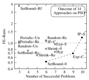
Figure 8: Performance comparison of 14 approaches for two metrics – number of problems solved successfully and function evaluation ratio – with the PSO algorithm.

The best approaches should have large $\rho_{j}$ values and small $\mbox{FE-ratio}_{j}$ values. This results in a trade-off between three best approaches which are marked in filled circles. All other 11 approaches are dominated by these three approaches. The SetBound (SetOnBoundary) with velocity set to zero performs in only six out of 12 problem instances. Thus, we ignore this approach. There is a clear trade-off between IP-S and Exp-C approaches. IP-S solves one problem more, but requires more FEs in comparison to Exp-C. Hence, we recommend the use of both of these methods vis-a-vis all other methods used in this study.

Other conclusions of this extensive study of PSO with different constraint-handling methods are summarized as follows:

1. The constraint-handling methods show a large variation in the performance depending on the choice of test problem and location of the optimum in the allowable variable range.

2. When the optimum is on the variable boundary, periodic and random allocation methods perform poorly. This is expected intuitively.

3. When the optimum is on the variable boundary, methods that set infeasible solutions on the violated boundary (SetOnBoundary methods) work very well for obvious reasons, but these methods do not perform well for other cases.

4. When the optimum lies near the center of the allowable range, most constraint-handling approaches work almost equally well. This can be understood intuitively from the fact that tendency of particles to fly out of the search space is small when the optimum is in the center of the allowable range. For example, the periodic approaches fail in all the cases but are able to demonstrate some convergence characteristics for all test problems, when the optimum is at the center. When the optimum is on the boundary or close to the boundary, then the effect of the chosen constraint-handling method becomes critical.

5. The shrink method (with “Velocity Recomputed” and “Velocity Set Zero” strategies) succeeded in 10 of the 12 cases.

4.2 Parametric Study of $\alpha$

The proposed IP approaches involve a parameter $\alpha$ affecting the variance of the probability distribution for the mapped variable. In this section, we perform a parametric study of $\alpha$ to determine its effect on the performance of the IP-S approach.

Following $\alpha$ values are chosen: $0.1$, $1$, $10$, and $1,000$. To have an idea of the effect of $\alpha$, we plot the probability distribution of mapped values in the allowable range ($[1,10]:OntheBoundary$) for $d=1.0$ in Figure 9. It can be seen that for $\alpha=10$ and 1,000, the distribution is almost uniform.

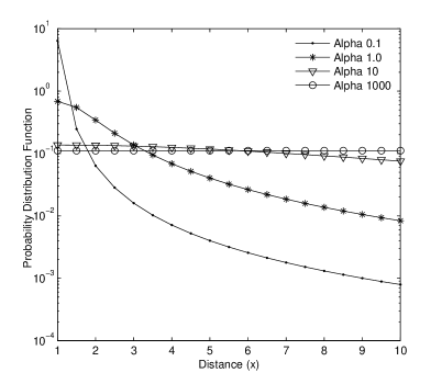
Figure 9: Probability distribution function with different $\alpha$ values. The $x$-axis denotes the increased distance from the violated boundary. $x=1$ means the violated boundary. The child is created at $x=0$.

Figure  10 shows the effect of $\alpha$ on $F_{elp}$ problem. For the same termination criterion we find that $\alpha=0.1$ and $1.0$ perform better compared to other values. With larger values of $\alpha$ the IP-S method does not even find the desired solution in all 50 runs.

Figure 10: Performance of PSO algorithm with the IP-S approach with different $\alpha$ values on $F_{elp}$ problem.

4.3 Results with Differential Evolution (DE)

Differential evolution, originally proposed in [24], has gained popularity as an efficient evolutionary optimization algorithm. The developers of DE proposed a total of ten different strategies [20]. In [2] it was shown that performance of DE largely depended upon the choice of constraint-handling mechanism. We use Strategy 1 (where the offspring is created around the population-best solution), which is most suited for solving unimodal problems [18]. A population size of $50$ was chosen with parameter values of $CR=0.5$ and $F=0.7$. Other parameters are set the same as before. We use $S=10^{-10}$ as our termination criterion. Results are tabulated in Tables 5 to  8. Following two observations can be drawn:

1. For problems having optimum at one of the boundaries, SetOnBoundary approach performs the best. This is not a surprising result.

2. However, for problems having the optimum near the center of the allowable range, almost all eight algorithms perform in a similar manner.

3. For problems having their optimum close to one of the boundaries, the proposed IP and existing exponential approaches perform better than the rest of the approaches with DE.

Despite the differences, somewhat similar performances of different constraint-handling approaches with DE indicates that the DE is an efficient optimization algorithm and its performance is somewhat less dependent on the choice of constraint-handling scheme compared to the PSO algorithm.

Table 5: Results on $F_{\rm elp}$ with DE for $10^{-10}$ termination criterion.

Strategy	Best	Median	Worst
$F_{\rm elp}$ in [0,10]: On the Boundary
IP Spread	25,600	26,850	27,650
IP Confined	22,400	23,550	24,200
Exp. Spread	38,350	39,800	41,500
Exp. Confined	19,200	20,700	21,900
Periodic	42,400	43,700	45,050
Random	40,650	43,050	44,250
SetOnBoundary	2,850	3,350	3,900
Shrink	4,050	4,900	5,850
$F_{\rm elp}$ in [-10,10]: At the Center
IP Spread	29,950	31,200	32,500
IP Confined	29,600	31,200	32,400
Exp. Spread	29,950	31,300	32,400
Exp. Confined	30,500	31,400	32,250
Periodic	29,650	31,300	32,400
Random	30,000	31,200	31,250
SetOnBoundary	29,850	31,200	32,700
Shrink	30,300	31,250	32,750
$F_{\rm elp}$ in [-1,10]: Close to Boundary
IP Spread	28,550	29,600	30,550
IP Confined	28,500	29,500	30,650
Exp. Spread	28,050	28,900	29,850
Exp. Confined	28,150	29,050	29,850
Periodic	29,850	30,850	32,100
Random	28,900	30,200	31,000
SetOnBoundary	28,650	29,600	30,500
Shrink	28,800	29,900	31,200

Table 6: Results on $F_{\rm sch}$ with DE for $10^{-10}$ termination criterion.

Strategy	Best	Median	Worst
$F_{\rm sch}$ in [0,10]: On the Boundary
IP Spread	26,600	27,400	28,000
IP Confined	22,450	23,350	24,300
Exp. Spread	40,500	42,050	43,200
Exp. Confined	19,650	20,350	22,050
Periodic	44,700	46,300	48,250
Random	43,850	45,150	47,000
SetOnBoundary	2,100	3,100	3,750
Shrink	3,450	4,400	5,100
$F_{\rm sch}$ in [-10,10]: At the Center
IP Spread	258,750	281,650	296,300
IP Confined	268,150	283,050	300,450
Exp. Spread	266,850	283,950	304,500
Exp. Confined	266,450	283,700	305,550
Periodic	269,700	284,100	310,100
Random	263,300	282,600	306,250
SetOnBoundary	267,750	284,550	298,850
Shrink	263,600	282,750	304,350
$F_{\rm sch}$ in [-1,10]: Close to Boundary
IP Spread	228,950	242,300	255,700
IP Confined	232,200	243,900	263,400
Exp. Spread	227,550	243,000	261,950
Exp. Confined	228,750	243,800	262,500
Periodic	231,950	247,150	260,700
Random	228,550	244,850	261,900
SetOnBoundary	237,100	255,750	266,400
Shrink	234,000	253,250	275,550

Table 7: Results on $F_{\rm ack}$ with DE for $10^{-10}$ termination criterion.

Strategy	Best	Median	Worst
$F_{\rm ack}$ in [0,10]: On the Boundary
IP Spread	43,400	44,950	45,950
IP Confined	37,300	38,700	40,350
Exp. Spread Dist.	66,300	69,250	71,300
Exp. Confined Dist	32,750	34,600	36,200
Periodic	72,500	74,250	75,900
Random	70,650	73,000	74,750
SetOnBoundary	2,550	3,250	3,950
Shrink	3,500	4,700	5,300
$F_{\rm ack}$ in [-10,10]: At the Center
IP Spread	50,650	52,050	53,450
IP Confined	51,050	52,200	53,800
Exp. Spread	51,200	52,150	53,400
Exp. Confined	51,100	52,300	53,850
Periodic	51,250	52,250	53,500
Random	50,950	52,200	53,450
SetOnBoundary	50,950	52,300	53,450
Shrink	50,450	52,300	53,550
$F_{\rm ack}$ in [-1,10]: Close to Boundary
IP Spread	49,100	50,650	51,650
IP Confined	48,650	50,400	52,100
Exp. Spread	48,300	49,900	51,750
Exp. Confined	48,900	50,000	51,250
Periodic	50,400	51,950	53,300
Random	50,250	51,200	52,150
SetOnBoundary	49,900 (33)	51,100	53,150
Shrink	50,200	51,400	52,750

Table 8: Results on $F_{\rm ros}$ with DE for $10^{-10}$ termination criterion.

Strategy	Best	Median	Worst
$F_{\rm ros}$ in [1,10]: On the Boundary
IP Spread	38,850	62,000	89,700
IP Confined	24,850	45,700	73,400
Exp. Spread	57,100	86,800	118,600
Exp. Confined	16,600	21,400	79,550
Periodic	69,550	93,500	18,1150
Random	65,850	92,950	157,600
SetOnBoundary	2,950	4,700	30,450
Shrink	5,450	8,150	55,550
$F_{\rm ros}$ in [-8,10]: At the Center
IP Spread	133,350 (41)	887,250	995,700
IP Confined	712,500 (44)	854,800	991,400
Exp. Spread	390,700 (48)	866,150	998,950
Exp. Confined	138,550 (40)	883,500	994,350
Periodic	764,650 (39)	874,700	999,650
Random	699,400 (49)	885,450	999,600
SetOnBoundary	743,600 (38)	865,450	995,500
Shrink	509,900 (40)	873,450	998,450
$F_{\rm ros}$ in [0,10]: Close to Boundary
IP Spread	36,850	78,700	949,700
IP Confined	46,400 (46)	95,900	891,450
Exp. Spread	49,550 (49)	85,900	968,200
Exp. Confined	87,300 (43)	829,200	973,350
Periodic	38,750	62,200	94,750
Random	41,200	61,300	461,500
SetOnBoundary	8.23E+00 (DNC)	1.62E+01	1.89E+01
Shrink	252,650 (9)	837,700	985,750

4.4 Results with Real-Parameter Genetic Algorithms (RGAs)

We have used two real-parameter GAs in our study here:

1. Standard-RGA using the simulated binary crossover (SBX) [9] operator and the polynomial mutation operator [8]. In this approach, variables are expressed as real numbers initialized within the allowable range of each variable. The SBX and polynomial mutation operators can create infeasible solutions. Violated boundary, if any, is handled using one of the approaches studied in this paper. Later we shall investigate a rigid boundary implementation of these operators which ensures creation of feasible solutions in every recombination and mutation operations.

2. Elitist-RGA in which two newly created offsprings are compared against the two parents, and the best two out of these four solutions are retained as parents (thereby introducing elitism). Here, the offspring solutions are created using non-rigid versions of SBX and polynomial mutation operators. As before, we test eight different constraint-handling approaches and, later explore a rigid boundary implementation of the operators in presence of elite preservation.

Parameters for RGAs are chosen as follows: population size of 100, crossover probability $p_{c}$=0.9, mutation probability $p_{m}$=0.05, distribution index for crossover $n_{dist.,c}$=2, distribution index for mutation $n_{dist.,m}$=100. The results for the Standard-RGA are shown in Tables 9 to  12 for four different test problems. Tables 13 to  16 show results using the Elitist-RGA. Following key observations can be made:

1. For all the four test problems, Standard-RGA shows convergence only in the situation when optima is on the boundary.

2. Elitist-RGA shows good convergence on $F_{elp}$ when the optimum is on the boundary and, only some convergence is noted when the optima is at the other locations. For other three problems, convergence is only obtained when optimum is present on the boundary.

3. Overall, the performance of Elite-RGA is comparable or slightly better compared to Standard-RGA.

The Did Not Converge cases can be explained on the fact that the SBX operator has the property of creating solutions around the parents; if parents are close to each other. This property is a likely cause of premature convergence as the population gets closer to the optima. Furthermore the results suggest that the elitism implemented in this study (parent-child comparison) is not quite effective.

Although RGAs are able to locate the optima, however, they are unable to fine-tune the optima due to undesired properties of the generation scheme. This emphasizes the fact that generation scheme is primarily responsible for creating good solutions, and the constraint-handling methods cannot act as surrogate for generating efficient solutions. Each step of the evolutionary search should be designed effectively in order to achieve overall success. On the other hand one could argue that strategies such as increasing the mutation rate (in order to promote diversity so as to avoid pre-mature convergence) should be tried, however, creation of good and meaningful solutions in the generation scheme is rather an important and a desired fundamental-feature.

As expected, when the optima is on the boundary SetOnBoundary finds the optima most efficiently within a minimum number of function evaluations. Like in PSO the performance of Exp. Confined is better than Exp. Spread. Periodic and Random show comparable or slightly worse performances (these mechanisms don’t have any preference of creating solutions close to the boundary and actually promote spread of the population).

Table 9: Results on $F_{\rm elp}$ with Standard-RGA for termination criterion of $10^{-10}$.

Strategy	Best	Median	Worst
$F_{\rm elp}$ in [0,10]
IP Spread	9,200	10,500	12,900
IP Confined	7,900	9,400	10,900
Exp. Spread	103,100 (6)	718,900	931,200
Exp. Confined	4,500	5,700	7,000
Periodic	15,200 (1)	15,200	15,200
Random	68,300 (12)	314,700	939,800
SetOnBoundary	1,800	2,400	2,800
Shrink	3,700	5,100	6,600
$F_{\rm elp}$ in [-10,10]
2.60e-02 (DNC)
$F_{\rm elp}$ in [-1,10]
1.02e-02 (DNC)

Table 10: Results on $F_{\rm sch}$ with Standard-RGA for termination criterion of $10^{-10}$

Strategy	Best	Median	Worst
$F_{\rm sch}$ in [0,10]
IP Spread	6,800	9,800	11,800
IP Confined	6,400	8,200	10,300
Exp. Spread	21,200 (47)	180,000	772,200
Exp. Confined	4,300	5,500	6,300
Periodic	14,800 (26)	143,500	499,400
Random	8,700 (43)	195,200	979,300
SetOnBoundary	1,800	2,300	2,900
Shrink.	3,600	4,600	5,500
$F_{\rm sch}$ in [-10,10]
1.20e-01 (DNC)
$F_{\rm sch}$ in [-1,10]
8.54e-02 (DNC)

Table 11: Results on $F_{\rm ack}$ with Standard-RGA for termination criterion of $10^{-10}$

Strategy	Best	Median	Worst
$F_{\rm ack}$ in [0,10]
IP Spread	12,100	22,600	43,400
IP Confined	9,800	13,200	16,400
Exp. Spread	58,100 (29)	355,900	994,000
Exp. Confined	6,300	9,100	11,900
Periodic	19,600 (46)	122,300	870,200
Random	35,700 (38)	229,200	989,500
SetOnBoundary	1,800	2,500	3,100
Shrink	4,200	5,700	8,600
$F_{\rm ack}$ in [-10,10]
7.76e-02(DNC)
$F_{\rm ack}$ in [-1,10]
4.00e-02 (DNC)

Table 12: Results on $F_{\rm ros}$ with Standard-RGA for termination criterion of $10^{-10}$

Strategy	Best	Median	Worst
$F_{\rm ros}$ in [1,10]: On the Boundary
IP Spread	12,400 (39)	15,800	20,000
IP Confined	9,400 (39)	11,800	13,600
Exp. Spread	9.73e+00 (DNC)	1.83e+00	2.43e+01
Exp. Confined	6,000	6,900	8,200
Periodic	6.30E+01 (DNC)	4.92e+02	5.27e+04
Random	3.97e+02 (DNC)	9.28e+02	1.50e+03
SetOnBoundary	1,900	2,700	3,400
Shrink	4,100	5,200	6,500
$F_{\rm ros}$ in [-8,10]
3.64e+00 (DNC)
$F_{\rm ros}$ in [1,10]: On the Boundary
1.04e+01(DNC)

Table 13: Results on $F_{\rm elp}$ with Elite-RGA for $10^{-10}$ termination criterion.

Strategy	Best	Median	Worst
$F_{\rm elp}$ in [0,10]
IP Spread	6,600	8,000	9,600
IP Confined	6,300	8,100	9,800
Exp. Spread	4,800	6,900	8,300
Exp. Confined	4,600	5,800	6,700
Periodic	6,500	8,800	11,500
Random	6,400	7,900	10,300
SetOnBoundary	2,200	2,600	3,500
Shrink	4,000	5,200	6,700
$F_{\rm elp}$ in [-10,10]
IP Spread	980,200 (1)	980,200	980,200
IP Confined	479,000 (1)	479,000	479,000
Exp. Spread	2.06e-01 (DNC)	4.53e-01	4.86e-01
Exp. Confined	954,400 (1)	954,400	954,400
Periodic	1.55E-01 (DNC)	2.48E-01	2.36E-01
Random	1.92E-01 (DNC)	2.00E-01	2.46E-01
SetOnBoundary	2.11E-01 (DNC)	2.95E-01	1.94E-01
Shrink	530,900 (3)	654,000	779,000
$F_{\rm elp}$ in [-1,10]
IP Spread	803,400 (5)	886,100	947,600
IP Confined	643,300 (2)	643,300	963,000
Exp. Spread	593,300 (3)	628,900	863,500
Exp. Confined	655,400 (3)	940,500	946,700
Periodic	653,800 (3)	842,900	843,100
Random	498,500 (2)	498,500	815,500
SetOnBoundary	593,800 (5)	870,500	993,500
Shrink	781,000 (2)	781,000	928,300

Table 14: Results on $F_{\rm sch}$ with Elite-RGA for termination criterion of $10^{-10}$

Strategy	Best	Median	Worst
$F_{\rm sch}$ in [0,10]
IP Spread	5,000	6,500	7,900
IP Confined	4,900	6,500	7,900
Exp. Spread	4,300	5,800	7,800
Exp. Confined	4,300	4,900	5,600
Periodic	5,400	7,000	11,300
Random	5,300	6,600	8,500
SetOnBoundary	1,600	2,200	2,600
Shrink	3,100	4,200	5,400
$F_{\rm sch}$ in [-10,10]
8.12e-05(DNC)
$F_{\rm sch}$ in [-1,10]
1.61e-01(DNC)

Table 15: Results on $F_{\rm ack}$ with Elite-RGA for termination criterion of $10^{-}{10}$

Strategy	Best	Median	Worst
$F_{\rm ack}$ in [0,10]
IP Spread	6,300	8,700	46,500
IP Confined	6,800	9,200	32,000
Exp. Spread	5,600	6,800	8,700
Exp. Confined	5,200	7,800	9,900
Periodic	6,300	9,300	12,200
Random	6,200	8,300	53,700
SetOnBoundary	1,900	2,500	4,000
Shrink	3,900	5,100	7,700
$F_{\rm ack}$ in [-10,10]
1.03e-01(DNC)
$F_{\rm ack}$ in [-1,10]
1.15e-00 (DNC)

Table 16: Results on $F_{\rm ros}$ with Elite-RGA for termination criterion of $10^{-}{10}$

Strategy	Best	Median	Worst
$F_{\rm ros}$ in [0,10]
IP Spread	9,900 (13)	12,500	14,000
IP Confined	10,100 (12)	12,100	14,400
Exp. Spread	8,500 (10)	11,000	15,400
Exp. Confined	6,600 (30)	7,800	8,900
Periodic	9,500 (10)	13,300	16,800
Random	14,000 (3)	15,300	16,100
SetOnBoundary	2,300 (44)	3,200	4,500
Shrink	4,500 (32)	6,100	8,100
$F_{\rm ros}$ in [-8,10]
1.27e-00 (DNC)
$F_{\rm ros}$ in [1,10]: On the Boundary
1.49e-00 (DNC)

4.4.1 RGAs with Rigid Boundary

Table 17: RGA with rigid boundary with termination criterion $10^{-10}$

Optimum on the boundary
Strategy	Best	Median	Worst
$F_{elp}$	8,100	8,500	8,800
$F_{sch}$	7,800	8,100	8,300
$F_{ack}$	9,500	10,100	10,800
$F_{ros}$	10,100 (39)	10,900	143,600
Optimum in the center
3.88e-02 (DNC)
Optimum close to the edge of the boundary
9.44e-03 (DNC)

We also tested RGA (standard and its elite version) with a rigid bound consideration in its operators. In this case, the probability distributions of both SBX and polynomial mutation operator are changed in a way so as to always create a feasible solution. It is found that the Standard-RGA with rigid bounds shows convergence only when optimum is on the boundary (Table 17). The performance of Elite-RGA with rigid bounds is slightly better (Table 18). Overall, SBX operating within the rigid bounds is found to perform slightly better compared to the RGAs employing boundary-handling mechanisms. However, as mentioned earlier, in the scenarios where the generation scheme cannot guarantee creation of feasible only solutions there is a necessary need for constraint-handling strategies.

Table 18: Elitist-RGA with rigid boundary with termination criterion $10^{-10}$.

Strategy	Best	Median	Worst
Optimum on the boundary
$F_{elp}$	7,300	7,900	8,400
$F_{sch}$	6,500	6,900	7,500
$F_{ack}$	9,400	10,400	12,200
$F_{ros}$	11000 (10)	12700	16400
Optimum in the center
1.24e-01(DNC)
Optimum close to the boundary edge
$F_{elp}$	579,800 (3)	885,900	908,600
$F_{sch}$	2.73E-00 DNC	6.18E-00	1.34E-00
$F_{ack}$	1.75E-01 DNC	8.38E-01	2.93E-00
$F_{ros}$	3.29E-00 DNC	4.91E+00	5.44E+00

5 Higher-Dimensional Problems

As the dimensionality of the search space increases it becomes difficult for a search algorithm to locate the optimum. Constraint-handling methods play even a more critical role in such cases. So far in this study, DE has been found to be the best algorithm. Next, we consider all four unimodal test problems with an increasing problem size: $n=20$, $50$, $100$, $200$, $300$, and $500$. For all problems the variable bounds were chosen such that optima occured near the center of the search space. No population scaling is used for DE. The DE parameters are chosen as $F=0.8$ and $CR=0.9$. For $\alpha=1.2$ we were able to achieve a high degree of convergence and results are shown in Figure 11. As seen from the figure, although it is expected that the required number of function evaluations would increase with the number of variables, the increase is sub-quadratic. Each case is run $20$ times and the termination criteria is set as $10^{-10}$. All 20 runs are found to be successful in each case, demonstrating the robustness of the method in terms of finding the optimum with a high precision. Particularly problems with large variables, complex search spaces and highly nonlinear constraints, such a methodology should be useful in terms of applying the method to different real-world problems.

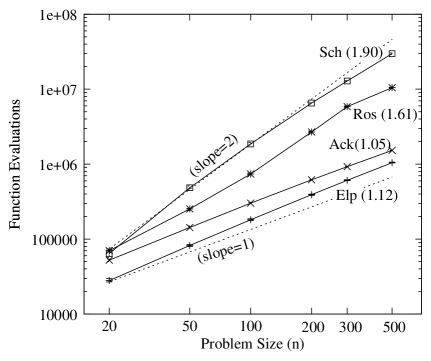
Figure 11: Scale-up study on four test problems for the DE algorithm with the proposed IP-S approach shows sub-quadratic performance in all problems. Slopes of a fitted polynomial line is marked within brackets for each problem. Linear and quadratic limit lines are shown with dashed lines.

It is worth mentioning that authors independently tested other scenarios for large scale problems with corresponding optimum on the boundary, and in order to achieve convergence with IP methods we had to significantly reduce the values of $\alpha$. Without lowering $\alpha$, particularly, PSO did not show any convergence. As expected in larger dimensions the probability to sample a point closer to the boundary decreases and hence a steeper distribution is needed. However, this highlights the usefulness of the parameter $\alpha$ to modify the behavior of the IPMs so as to yield the desired performance.

6 General Purpose Constraint-Handling

So far we have carried out simulations on problems where constraints have manifested as the variable bounds. The IP methods proposed in this paper can be easily extended and employed for solving nonlinear constrained optimization problems (inclusive of variable bounds).

As an example, let us consider a generic inequality constraint function: $g_{j}(\vec{x})\geq 0$ – the $j$-th constraint in a set of $J$ inequality constraints. In an optimization algorithm, every created (offspring) solution $\vec{x}^{c}$ at an iteration must be checked for its feasibility. If $\vec{x}^{c}$ satisfies all $J$ inequality constraints, the solution is feasible and the algorithm can proceed with the created solution. But if $\vec{x}^{c}$ does not satisfy one or more of $J$ constraints, the solution is infeasible and should be repaired before proceeding further.

Let us illustrate the procedure using the inverse parabolic (IP) approach described in Section 3; though other constraint-handling methods discussed before may also be used. The IP approaches require us to locate intersection points $\vec{v}$ and $\vec{u}$: two bounds in the direction of ($\vec{x}^{p}-\vec{x}^{c}$), where $\vec{x}^{p}$ is one of the parent solutions that created the offspring solution (see Figure 12). The critical intersection point can be found by finding multiple roots of the direction vector with each constraint $g_{j}(\vec{x})$ and then choosing the smallest root.

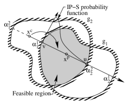
Figure 12: Extension of constraint-handling approaches to constrained optimization problems.

We define a parameter $\alpha$ as the extent of a point from $\vec{x}^{c}$, as follows:

$$\vec{x}(\alpha)=\vec{x}^{c}+\alpha\frac{\vec{x}^{p}-\vec{x}^{c}}{\|\vec{x}^{p}-\vec{x}^{c}\|}.$$ (19)

Substituting above expression for $\vec{x}(\alpha)$ in the $j$-th constraint function, we have the following root-finding problem for the $j$-th constraint:

$$g_{j}(\vec{x}(\alpha))=0.$$ (20)

Let us say the roots of the above equation are $\alpha_{k}^{j}$ for $k=1,2\ldots,K_{j}$. The above procedure can now be repeated for all $J$ inequality constraints and corresponding roots can be found one at a time. Since the extent of $\alpha$ to reach $\vec{x}^{p}$ from $\vec{x}^{c}$ is given as

$$\alpha^{p}=\|\vec{x}^{p}-\vec{x}^{c}\|,$$

we are now ready to compute the two closest bounds (lower and upper bounds) on $\alpha$ for our consideration, as follows:

$$\alpha^{v} = \max\{\alpha_{k}^{j}|0\leq\alpha_{k}^{j}\leq\alpha^{p},\forall k,\forall j\},$$ (21)

$$\alpha^{u} = \min\{\alpha_{k}^{j}|\alpha_{k}^{j}\geq\alpha^{p},\forall k,\forall j\}.$$ (22)

IP-S and IP-C approaches presented in Section 3 now can be used to map the violated variable value $x_{i}^{c}$ into the feasible region using $d=\alpha^{v}$ (the lower bound), $d_{u}=\alpha^{u}$ (the upper bound) and $d^{p}=\alpha^{p}$ (location of parent). It is clear that the only difficult aspect of this method is to find multiple intersection points in presence of nonlinear constraints.

For the sake of completeness, we show here that the two bounds for each variable: $x_{i}\geq x_{i}^{(L)}$ and $x_{i}\leq x_{i}^{(U)}$ used in previous sections can be also be treated uniformly using the above described approach. The two bounds can be written together as follows:

$$\left(x_{i}-x_{i}^{(L)}\right)\left(x_{i}^{(U)}-x_{i}\right)\geq 0.$$ (23)

Note that a simultaneous non-positive value of each of the bracketed terms is not possible, thus only way to satisfy the above left side is to make each bracketed term non-negative. The above inequality can be considered as a quadratic constraint function, instead of two independent variable bounds and treated as a single combined nonlinear constraint and by finding both roots of the resulting quadratic root-finding equation.

Finally, the above procedure can also be extended to handle equality constraints ($h_{k}(\vec{x})=0$) with a relaxation as follows: $-\epsilon_{k}\leq h_{k}(\vec{x})\leq\epsilon_{k}$. Again, they can be combined together as follows:

$$\epsilon_{k}^{2}-(h_{k}(\vec{x}))^{2}\geq 0.$$ (24)

Alternatively, the above can also be written as $\epsilon_{k}-|h_{k}(\vec{x})|\geq 0$ and may be useful for non-gradient based optimization methods, such as evolutionary algorithms. We now show the working of the above constraint handling procedure on a number of constrained optimization problems.

6.1 Illustrations on Nonlinear Constrained Optimization

First, we consider the three unconstrained problems used in previous sections as $f(\vec{x})$, but now add an inequality constraint by imposing a quadratic constraint that makes the solutions fall within a radius of one-unit from a chosen point $\vec{o}$:

$$\begin{array}[]{rl}\mbox{Minimize}&f(\vec{x}),\\ \mbox{subject to}&\sum_{i=1}^{n}(x_{i}-o_{i})^{2}\leq 1.\end{array}$$ (25)

There are no explicit variable bounds in the above problem. By choosing different locations of the center of the hyper-sphere ($\vec{o}$), we can have different scenarios of the resulting constrained optimum. If the minimum of the objective function (without constraints) lies at the origin, then setting $o_{i}=0$ the unconstrained minimum is also the solution to the constrained problem, and this case is similar to the “Optimum at the Center” (but in the context of constrained optimization now). The optimal solution is at $x_{i}=0$ with $f^{*}=0$. DE with IP-S and previous parameter settings is applied to this new constrained problem, and the results from 50 different runs for this case are shown in Table 19.

Table 19: Results for test functions with DE for $o_{i}=0$ with $S=10^{-10}$.

Strategy	Best	Median	Worst
$F_{\rm elp}$	22,800	23,750	24,950
$F_{\rm sch}$	183,750	206,000	229,150
$F_{\rm ack}$	42,800	44,250	45,500

As a next case, we consider $o_{i}=2$. The constrained minimum is now different from that of the unconstrained problem, as the original unconstrained minimum is no more feasible. This case is equivalent to “Optima on the Constraint Boundary”. Since the optimum value is not zero as before, instead of choosing a termination criterion based on $S$ value, we allocate a maximum of one million function evaluations for a run and record the obtained optimized solution. The best fitness values for $f(\vec{x})$ as $f_{elp}$, $f_{sch}$ and $f_{ack}$ are shown in Table  20. For each function, we verified that the obtained optimized solution satisfies the KKT optimality conditions [22, 5] suggesting that a truly optimum solution has been found by this procedure.

Table 20: Best fitness results for test functions with DE for $o_{i}=2$.

$F_{\rm elp}$	$F_{\rm sch}$	$F_{\rm ack}$
640.93 $\pm$ 0.00	8871.06 $\pm$ 0.39	6.56 $\pm$ 0.00

Next, we consider two additional nonlinear constrained optimization problems (TP5 and TP8) from [7] and a well-studied structural design and mechanics problem (‘Weld’) taken from [21]. The details on the mechanics of the welded structure and the beam deformation can be found in [23, 25]. These problems have multiple nonlinear inequality constraints and our goal is to demonstrate the performance of our proposed constraint-handling methods. We used DE with IP-S method with the following parameter settings: $NP=50$, $F=0.7$, $CR=0.5$, and $\alpha=1.2$ for all three problems. A maximum of 200,000 function evaluations were allowed and a termination criteria of $10^{-3}$ from the known optima is chosen. The problem definitions of TP5, TP8 and ‘Weld’ are as follows:

TP5:

$$\begin{array}[]{rl}\mbox{Minimize}&f(\vec{x})=(x_{1}-10)^{2}+5(x_{2}-12)^{2}+x_{3}^{4}+3(x_{4}-11)^{2}\\ &\qquad+10x_{5}^{6}+7x_{6}^{2}+x^{4}_{7}-4x_{6}x_{7}-10x_{6}-8x_{7},\\ \mbox{subject to}&g_{1}(\vec{x})\equiv 2x_{1}^{2}+3x_{2}^{4}+x_{3}+4x_{4}^{2}+5x_{5}\leq 127,\\ &g_{2}(\vec{x})\equiv 7x_{1}+3x_{2}+10x_{3}^{2}+x_{4}-x_{5}\leq 282,\\ &g_{3}(\vec{x})\equiv 23x_{1}+x_{2}^{2}+6x_{6}^{2}-8x_{7}\leq 196,\\ &g_{4}(\vec{x})\equiv 4x_{1}^{2}+x_{2}^{2}-3x_{1}x_{2}+2x_{3}^{2}+5x_{6}-11x_{7}\leq 0,\\ &-10\leq x_{i}\leq 10,\quad i=1,\ldots,7.\end{array}$$ (26)

TP8:

$$\begin{array}[]{rl}\mbox{Minimize}&f(\vec{x})=x_{1}^{2}+x_{2}^{2}+x_{1}x_{2}-14x_{1}-16x_{2}+2(x_{9}-10)^{2}\\ &\qquad+2(x_{6}-1)^{2}+5x_{7}^{2}+7(x_{8}-11)^{2}+45+(x_{10}-7)^{2}\\ &\qquad+(x_{3}-10)^{2}+4(x_{4}-5)^{2}+(x_{5}-3)^{2}\\ \mbox{subject to}&g_{1}(\vec{x})\equiv 4x_{1}+5x_{2}-3x_{7}+9x_{8}\leq 105,\\ &g_{2}(\vec{x})\equiv 10x_{1}-8x_{2}-17x_{7}+2x_{8}\leq 0,\\ &g_{3}(\vec{x})\equiv-8x_{1}+2x_{2}+5x_{9}-2x_{10}\leq 12,\\ &g_{4}(\vec{x})\equiv 3(x_{1}-2)^{2}+4(x_{2}-3)^{2}+2x_{3}^{2}-7x_{4}\leq 120,\\ &g_{5}(\vec{x})\equiv 5x_{1}^{2}+8x_{2}+(x_{3}-6)^{2}-2x_{4}\leq 40,\\ &g_{6}(\vec{x})\equiv x_{1}^{2}+2(x_{2}-2)^{2}-2x_{1}x_{2}+14x_{5}-6x_{6}\leq 0,\\ &g_{7}(\vec{x})\equiv 0.5(x_{1}-8)^{2}+2(x_{2}-4)^{2}+3x_{5}^{2}-x_{6}\leq 30,\\ &g_{8}(\vec{x})\equiv-3x_{1}+6x_{2}+12(x_{9}-8)^{2}-7x_{10}\leq 0,\\ &-10\leq x_{i}\leq 10,\quad i=1,\ldots,10.\end{array}$$ (27)

‘Weld’:

$$\begin{array}[]{rl}\mbox{Minimize}&f(\vec{x})=1.10471h^{2}l+0.04811tb(14.0+l),\\ \mbox{subject to}&g_{1}(\vec{x})\equiv\tau(\vec{x})\leq 13,600,\\ &g_{2}(\vec{x})\equiv\sigma(\vec{x})\leq 30,000,\\ &g_{3}(\vec{x})\equiv h-b\leq 0,\\ &g_{4}(\vec{x})\equiv P_{c}(\vec{x})\geq 6,000,\\ &g_{5}(\vec{x})\equiv\delta(\vec{x})\leq 0.25,\\ &0.125\leq(h,b)\leq 5,\mbox{ and }0.1\leq(l,t)\leq 10,\end{array}$$ (28)

where,

$$\tau(\vec{x}) = \sqrt{(\tau^{\prime})^{2}+(\tau^{\prime\prime})^{2}+(l\tau^{\prime}\tau^{\prime\prime})/\sqrt{0.25(l^{2}+(h+t)^{2})}},$$

$$\tau^{\prime} = \frac{6,000}{\sqrt{2}hl},$$

$$\tau^{\prime\prime} = \frac{6,000(14+0.5l)\sqrt{0.25*(l^{2}+(h+t)^{2})}}{2[0.707hl(l^{2}/12+0.25(h+t)^{2})]},$$

$$\sigma(\vec{x}) = \frac{504,000}{t^{2}b},$$

$$\delta(\vec{x}) = \frac{2.1952}{t^{3}b},$$

$$P_{c}(\vec{x}) = 64,746.022(1-0.0282346t)tb^{3}.$$

The feasible region in the above problems is quite complex, unlike hypercubes in case of problems with variable bounds, and since our methods require feasible initial population, we first identified a single feasible-seed solution (known as the seed solution), and generated other several other random solutions. Amongst the several randomly generated solutions, those infeasible, were brought into the feasible region using IP-S method and feasible-seed solution as the reference. The optimum results for TP5, TP8 and ‘Weld’, thus found, are shown in the Table 21.

Table 21: Results from TP5, TP8 and ‘Weld’ problem. For each problem, the obtained solution also satisfies the KKT conditions.

	Optimum Value ($f^{*}$)	Corresponding Solution Vector ($\vec{x}^{\ast}$)	Active Constraints
TP5	$680.63$	$(2.330,1.953,-0.473,4.362,-0.628,1.035,1.591)^{T}$	$g_{1}$, $g_{4}$
TP8	$24.33$	$(2.160,2.393,8.777,5.088,0.999,1.437,1.298,9.810,8.209,8.277)^{T}$	$g_{1}$ to $g_{6}$
‘Weld’	$2.38$	$(0.244,6.219,8.291,0.244)^{T}$	$g_{1}$ to $g_{4}$

To verify the obtained optimality of our solutions, we employed MATLAB sequential quadratic programming (SQP) toolbox with a termination criterion of $10^{-6}$ to solve each of the three problems. The solution obtained from SQP method matches with our reported solution indicating that our proposed constrained handling procedure is successful in solving the above problems.

Finally, the convergence plots of a sample run on these test problems is shown in Figures 13, 14, and 15, respectively. From the graphs it is clear that our proposed method is able to converge to the final solution quite effectively.

Figure 13: Convergence plot for TP5.

Figure 14: Convergence plot for TP8.

Figure 15: Convergence plot for TP8.

7 Conclusions

The existing constraint-handling strategies that repair solutions by bringing them back into the search spaces exhibit several inadequacies. This paper has addressed the task of studying, and proposing two new, explicit feasibility preserving constraint-handling methods for real-parameter optimization using evolutionary algorithms. Our proposed single parameter Inverse Parabolic Methods with stochastic and adaptive components, overcome limitations of existing methods and perform effectively on several test problems. Empirical comparisons on four different benchmark test problems ($F_{elp}$, $F_{sch}$, $F_{ack}$, and $F_{ros}$) with three different settings of the optimum relative to the variable boundaries revealed key insights into the performance of PSO, GAs and DE in conjunction with different constraint-handling strategies. It was noted that in addition to the critical role of constraint-handling strategy (which is primarily responsible for bringing the infeasible solutions back into the search space), the generation scheme (child-creation step) in an evolutionary algorithm must create efficient solutions in order to proceed effectively. Exponential and Inverse Parabolic Methods were most robust methods and never failed to solve any problem. The other constraint-handling strategies were either too deterministic and/or operated without utilizing sufficient useful information from the solutions. The probabilistic methods were able to bring the solutions back into the feasible part of the search space and showed a consistent performance. In particular, scale-up studies on four problems, up to 500 variables, demonstrated sub-quadratic empirical run-time complexity with the proposed IP-S method.

Finally, the success of the proposed IP-S scheme is demonstrated on generalized nonlinear constrained optimization problems. For such problems, the IP-S method requires finding the lower and upper bounds for feasible region along the direction of search by solving a series of root-finding problems. To best of our knowledge, the proposed constraint-handling approach is a first explicit feasibility preserving method that has demonstrated success on optimization problems with variable bounds and nonlinear constraints. The approach is arguably general, and can be applied with complex real-parameter search spaces such as non-convex, discontinuous, etc., in addition to problems dealing with multiple conflicting objectives, multi-modalities, dynamic objective functions, and other complexities. We expect that proposed constraint-handling scheme will find its utility in solving complex real-world constrained optimization problems using evolutionary algorithms. An interesting direction for the future would be to carry out one-to-one comparison between evolutionary methods employing constrained handling strategies and the classical constrained optimization algorithms. Such studies shall benefit the practitioners in optimization to compare and evaluate different algorithms in a unified frame-work. In particular, further development of a robust, parameter-less and explicit feasibility preserving constraint-handling procedure can be attempted. Other probability distribution functions and utilizing of information from other solutions of the population can also be attempted.

References

- [1] J. E. Alvarez-Benitez, R. M. Everson, and J. E. Fieldsend. A MOPSO algorithm based exclusively on pareto dominance concepts. In EMO, volume 3410, pages 459–473, 2005.
- [2] Jarosłlaw Arabas, Adam Szczepankiewicz, and Tomasz Wroniak. Experimental comparison of methods to handle boundary constraints in differential evolution. In Parallel Problem Solving from Nature, PPSN XI, volume 6239 of Lecture Notes in Computer Science, pages 411–420. Springer Berlin / Heidelberg, 2010.
- [3] Wei Chu, Xiaogang Gao, and Soroosh Sorooshian. Handling boundary constraints for particle swarm optimization in high-dimensional search space. Information Sciences, 181(20):4569 – 4581, 2011.
- [4] Rituparna Datta and Kalyanmoy Deb. A bi-objective based hybrid evolutionary-classical algorithm for handling equality constraints. In Ricardo H.C. Takahashi, Kalyanmoy Deb, Elizabeth F. Wanner, and Salvatore Greco, editors, Evolutionary Multi-Criterion Optimization, volume 6576 of Lecture Notes in Computer Science, pages 313–327. Springer Berlin Heidelberg, 2011.
- [5] Kalyanmoy Deb. Optimization for Engineering Design: Algorithms and Examples. Prentice-Hall, New Delhi, 1995.
- [6] Kalyanmoy Deb. Simulated binary crossover for continuous search space. Complex Systems, 9:115–148, 1995.
- [7] Kalyanmoy Deb. An efficient constraint handling method for genetic algorithms. Computer Methods in Applied Mechanics and Engineering, 186(2–4):311 – 338, 2000.
- [8] Kalyanmoy Deb. Multi-Objective Optimization using Evolutionary Algorithms. WILEY, 2002.
- [9] Kalyanmoy Deb and Ram Bhushan Agrawal. Simulated binary crossover for continuous search space. Complex Systems, 9:1–34, 1994.
- [10] AmirHossein Gandomi and Xin-She Yang. Evolutionary boundary constraint handling scheme. Neural Computing and Applications, 21(6):1449–1462, 2012.
- [11] S. Helwig, J. Branke, and S.M. Mostaghim. Experimental analysis of bound handling techniques in particle swarm optimization. Evolutionary Computation, IEEE Transactions on, 17(2):259–271, 2013.
- [12] S. Helwig and R. Wanka. Particle swarm optimizatio in high-dimensional bounded search spaces. In Proceedings of the 2007 IEEE Swarm Intelligence Symposium, pages 198–205.
- [13] Paul A Jensen and Jonathan F Bard. Operations research models and methods. John Wiley & Sons Incorporated, 2003.
- [14] Zbigniew Michalewicz. A Survey of Constraint Handling Techniques in Evolutionary Computation Methods.
- [15] Zbigniew Michalewicz and Cezary Z. Janikow. Genocop: a genetic algorithm for numerical optimization problems with linear constraints. Communications of the ACM, 39(12es):175, 1996.
- [16] N. Padhye, J. Branke, and S. Mostaghim. Empirical comparison of mopso methods - guide selection and diversity preservation -. In Proceedings of CEC, pages 2516 – 2523. IEEE, 2009.
- [17] Nikhil Padhye. Development of efficient particle swarm optimizers and bound handling methods. Master’s thesis, IIT Kanpur, India, 2010.
- [18] Nikhil Padhye, Piyush Bhardawaj, and Kalyanmoy Deb. Improving differential evolution through a unified approach. Journal of Global Optimization, pages 1–29, 2012.
- [19] Nikhil Padhye, Kalyanmoy Deb, and Pulkit Mittal. Boundary handling approaches in particle swarm optimization. In Proceedings of Bio-Inspired Computing:Theories and Applications (BIC-TA 2012), pages 287–298, 2013.
- [20] Kenneth V. Price, Rainer M. Storn, and Jouni A. Lampinen. Differential Evolution: a practical approach to global optimization. Springer-Verlag, Hiedelberg, 2005.
- [21] KM Ragsdell and DT Phillips. Optimal design of a class of welded structures using geometric programming. Journal of Manufacturing Science and Engineering, 98(3):1021–1025, 1976.
- [22] G. V. Reklaitis, A. Ravindran, and K. M. Ragsdell. Engineering Optimization Methods and Applications. Willey, New York, 1983.
- [23] Joseph Edward Shigley. Engineering design. McGraw-Hill, 1963.
- [24] R. Storn and K. Price. Differential evolution – a simple and efficient heuristic for global optimization over continuous spaces. J. of Global Optimization, 11(4):341–359, 1997.
- [25] Stephen P Timoshenko, James M Gere, and W Prager. Theory of elastic stability. Journal of Applied Mechanics, 29:220, 1962.
- [26] Yong Wang and Zixing Cai. Combining multiobjective optimization with differential evolution to solve constrained optimization problems. Evolutionary Computation, IEEE Transactions on, 16(1):117–134, 2012.
- [27] Yong Wang and Zixing Cai. A dynamic hybrid framework for constrained evolutionary optimization. Systems, Man, and Cybernetics, Part B: Cybernetics, IEEE Transactions on, 42(1):203–217, 2012.
- [28] Guns Zoutendyk. Methods of feasible directions. Elsevier, 1960.