Mini-Batch Semi-Stochastic Gradient Descent
in the Proximal Setting

Abstract

We propose mS2GD: a method incorporating a mini-batching scheme for improving the theoretical complexity and practical performance of semi-stochastic gradient descent (S2GD). We consider the problem of minimizing a strongly convex function represented as the sum of an average of a large number of smooth convex functions, and a simple nonsmooth convex regularizer. Our method first performs a deterministic step (computation of the gradient of the objective function at the starting point), followed by a large number of stochastic steps. The process is repeated a few times with the last iterate becoming the new starting point. The novelty of our method is in introduction of mini-batching into the computation of stochastic steps. In each step, instead of choosing a single function, we sample $b$ functions, compute their gradients, and compute the direction based on this. We analyze the complexity of the method and show that it benefits from two speedup effects. First, we prove that as long as $b$ is below a certain threshold, we can reach any predefined accuracy with less overall work than without mini-batching. Second, our mini-batching scheme admits a simple parallel implementation, and hence is suitable for further acceleration by parallelization.

I Introduction

In this work we are concerned with the problem of minimizing the sum of two convex functions,

$$\min_{{x}\in\mathbb{R}^{d}}\{P({x}):=F({x})+R({x})\},$$ (1)

where the first component, $F$, is smooth, and the second component, $R$, is possibly nonsmooth (and extended real-valued, which allows for the modeling of constraints).

In the last decade, an intensive amount of research was conducted into algorithms for solving problems of the form (1), largely motivated by the realization that the underlying problem has a considerable modeling power. One of the most popular and practical methods for (1) is the accelerated proximal gradient method of Nesterov [1], with its most successful variant being FISTA [2].

In many applications in optimization, signal processing and machine learning, $F$ has an additional structure. In particular, it is often the case that $F$ is the average of a number of convex functions:

$$F({x})=\frac{1}{n}\sum_{i=1}^{n}f_{i}({x}).$$ (2)

Indeed, even one of the most basic optimization problems—least squares regression—lends itself to a natural representation of the form (2).

I-A Stochastic methods.

For problems of the form (1)+(2), and especially when $n$ is large and when a solution of low to medium accuracy is sufficient, deterministic methods do not perform as well as classical stochastic methods. The prototype method in this category is stochastic gradient descent (SGD), dating back to the 1951 seminal work of Robbins and Monro [3]. SGD selects an index $i\in\{1,2,\dots,n\}$ uniformly at random, and then updates the variable ${x}$ using $\nabla f_{i}({x})$ — a stochastic estimate of $\nabla F({x})$. Note that the computation of $\nabla f_{i}$ is $n$ times cheaper than the computation of the full gradient $\nabla F$. For problems where $n$ is very large, the per-iteration savings can be extremely large, spanning several orders of magnitude.

These savings do not come for free, however (modern methods, such as the one we propose, overcome this – more on that below). Indeed, the stochastic estimate of the gradient embodied by $\nabla f_{i}$ has a non-vanishing variance. To see this, notice that even when started from an optimal solution $x_{*}$, there is no reason for $\nabla f_{i}(x_{*})$ to be zero, which means that SGD drives away from the optimal point. Traditionally, there have been two ways of dealing with this issue. The first one consists in choosing a decreasing sequence of stepsizes. However, this means that a much larger number of iterations is needed. A second approach is to use a subset (“minibatch”) of indices $i$, as opposed to a single index, in order to form a better stochastic estimate of the gradient. However, this results in a method which performs more work per iteration. In summary, while traditional approaches manage to decrease the variance in the stochastic estimate, this comes at a cost.

I-B Modern stochastic methods

Very recently, starting with the SAG [4], SDCA [5], SVRG [6] and S2GD [7] algorithms from year 2013, it has transpired that neither decreasing stepsizes nor mini-batching are necessary to resolve the non-vanishing variance issue inherent in the vanilla SGD methods. Instead, these modern stochastic method are able to dramatically improve upon SGD in various different ways, but without having to resort to the usual variance-reduction techniques (such as decreasing stepsizes or mini-batching) which carry with them considerable costs drastically reducing their power. Instead, these modern methods were able to improve upon SGD without any unwelcome side effects. This development led to a revolution in the area of first order methods for solving problem (1)+(2). Both the theoretical complexity and practical efficiency of these modern methods vastly outperform prior gradient-type methods.

In order to achieve $\epsilon$-accuracy, that is,

$$\operatorname{\mathbf{E}}[P(x_{k})-P(x_{*})]\leq\epsilon[P(x_{0})-P(x_{*})],$$ (3)

modern stochastic methods such as SAG, SDCA, SVRG and S2GD require only

$${\cal O}((n+\kappa)\log(1/\epsilon))$$ (4)

units of work, where $\kappa$ is a condition number associated with $F$, and one unit of work corresponds to the computation of the gradient of $f_{i}$ for a random index $i$, followed by a call to a prox-mapping involving $R$. More specifically, $\kappa=L/\mu$, where $L$ is a uniform bound on the Lipschitz constants of the gradients of functions $f_{i}$ and $\mu$ is the strong convexity constant of $P$. These quantities will be defined precisely in Section IV.

The complexity bound (4) should be contrasted with that of proximal gradient descent (e.g., ISTA), which requires $O(n\kappa\log(1/\epsilon))$ units of work, or FISTA, which requires $O(n\sqrt{\kappa}\log(1/\epsilon))$ units of work. Note that while all these methods enjoy linear convergence rate, the modern stochastic methods can be many orders of magnitude faster than classical deterministic methods. Indeed, one can have

$$n+\kappa\ll n\sqrt{\kappa}\leq n\kappa.$$

Based on this, we see that these modern methods always beat (proximal) gradient descent ($n+\kappa\ll n\kappa$), and also outperform FISTA as long as $\kappa\leq{\cal O}(n^{2})$. In machine learning, for instance, one usually has $\kappa\approx n$, in which case the improvement is by a factor of $\sqrt{n}$ when compared to FISTA, and by a factor of $n$ over ISTA. For applications where $n$ is massive, these improvements are indeed dramatic.

For more information about modern dual and primal methods we refer the reader to the literature on randomized coordinate descent methods [8, 9, 10, 11, 12, 5, 13, 14, 15, 16, 17, 18] and stochastic gradient methods [4, 19, 20, 21, 22, 23, 17, 24], respectively.

I-C Linear systems and sketching.

In the case when $R\equiv 0$, all stationary points (i.e., points satisfying $\nabla F(x)=0$) are optimal for (1)+(2). In the special case when the functions $f_{i}$ are convex quadratics of the form $f_{i}(x)=\tfrac{1}{2}(a_{i}^{T}x-b_{i})$, the equation $\nabla F(x)=0$ reduces to the linear system $A^{T}Ax=A^{T}b$, where $A=[a_{1},\dots,n]$. Recently, there has been considerable interest in designing and analyzing randomized methods for solving linear systems; also known under the name of sketching methods. Much of this work was done independently from the developments in (non-quadratic) optimization, despite the above connection between optimization and linear systems. A randomized version of the classical Kaczmarz method was studied in a seminal paper by Strohmer and Vershynin [25]. Subsequently, the method was extended and improved upon in several ways [26, 27, 28, 29]. The randomized Kaczmarz method is equivalent to SGD with a specific stepsize choice [30, 31]. The first randomized coordinate descent method, for linear systems, was analyzed by Lewis and Leventhal [32], and subsequently generalized in various ways by numerous authors (we refer the reader to [17] and the references therein). Gower and Richtárik [31] have recently studied randomized iterative methods for linear systems in a general sketch and project framework, which in special cases includes randomized Kaczmarz, randomized coordinate descent, Gaussian descent, randomized Newton, their block variants, variants with importance sampling, and also an infinite array of new specific methods. For approaches of a combinatorial flavour, specific to diagonally dominant systems, we refer to the influential work of Spielman and Teng [33].

II Contributions

In this paper we equip moderns stochastic methods—methods which already enjoy the fast rate (4)—with the ability to process data in mini-batches. None of the primal modern methods have been analyzed in the mini-batch setting. This paper fills this gap in the literature.

While we have argued above that the modern methods, S2GD included, do not have the “non-vanishing variance” issue that SGD does, and hence do not need mini-batching for that purpose, mini-batching is still useful. In particular, we develop and analyze the complexity of mS2GD (Algorithm 1) — a mini-batch proximal variant of semi-stochastic gradient descent (S2GD) [7]. While the S2GD method was analyzed in the $R=0$ case only, we develop and analyze our method in the proximal setting (1). We show that mS2GD enjoys several benefits when compared to previous modern methods. First, it trivially admits a parallel implementation, and hence enjoys a speedup in clocktime in an HPC environment. This is critical for applications with massive datasets and is the main motivation and advantage of our method. Second, our results show that in order to attain a specified accuracy $\epsilon$, mS2GD can get by with fewer gradient evaluations than S2GD. This is formalized in Theorem 2, which predicts more than linear speedup up to a certain threshold mini-batch size after which the complexity deteriorates. Third, compared to [35], our method does not need to average the iterates produced in each inner loop; we instead simply continue from the last one. This is the approach employed in S2GD [7].

III The Algorithm

In this section we first briefly motivate the mathematical setup of deterministic and stochastic proximal gradient methods in Section IIIA, followed by the introduction of semi-stochastic gradient descent in Section IIIB. We will the be ready to describe the mS2GD method in Section IIIC.

III-A Deterministic and stochastic proximal gradient methods

The classical deterministic proximal gradient approach [2, 36, 37] to solving (1) is to form a sequence $\{{y}_{t}\}$ via

$${y}_{t+1}=\arg\min_{{x}\in\mathbb{R}^{d}}U_{t}(x),$$

where $U_{t}(x)\stackrel{{\scriptstyle\text{def}}}{{=}}F({y}_{t})+\nabla F({y}_{t})^{T}({x}-{y}_{t})+\tfrac{1}{2h}\|{x}-{y}_{t}\|^{2}+R(x)$. Note that in view of Assumption 1, which we shall use in our analysis in Section IV, $U_{t}$ is an upper bound on $P$ whenever $h>0$ is a stepsize parameter satisfying $1/h\geq L$. This procedure can be compactly written using the proximal operator as follows:

$${y}_{t+1}=\operatorname{prox}_{hR}({y}_{t}-h\nabla F({y}_{t})),$$

where

$$\operatorname{prox}_{hR}({z})\stackrel{{\scriptstyle\text{def}}}{{=}}\arg\min_{{x}\in\mathbb{R}^{d}}\{\tfrac{1}{2}\|{x}-{z}\|^{2}+hR({x})\}.$$

In a large-scale setting it is more efficient to instead consider the stochastic proximal gradient approach, in which the proximal operator is applied to a stochastic gradient step:

$$y_{t+1}=\operatorname{prox}_{hR}(y_{t}-hG_{t}),$$ (5)

where $G_{t}$ is a stochastic estimate of the gradient $\nabla F(y_{t})$.

III-B Semi-stochastic methods

Of particular relevance to our work are the SVRG [6], S2GD [7] and Prox-SVRG [35] methods where the stochastic estimate of $\nabla F(y_{t})$ is of the form

$$G_{t}=\nabla F(x)+\tfrac{1}{nq_{i_{t}}}(\nabla f_{i_{t}}({y}_{t})-\nabla f_{i_{t}}(x)),$$ (6)

where $x$ is an “old” reference point for which the gradient $\nabla F(x)$ was already computed in the past, and $i_{t}\in[n]\stackrel{{\scriptstyle\text{def}}}{{=}}\{1,2,\dots,n\}$ is a random index equal to $i$ with probability $q_{i}>0$. Notice that $G_{t}$ is an unbiased estimate of the gradient of $F$ at $y_{t}$:

$$\operatorname{\mathbf{E}}_{i_{t}}[G_{t}]\overset{\eqref{eq:sjs8js}}{=}\nabla F(x)+\sum_{i=1}^{n}q_{i}\tfrac{1}{nq_{i}}(\nabla f_{i}(y_{t})-\nabla f_{i}(x))\overset{\eqref{Px2}}{=}\nabla F(y_{t}).$$

Methods such as S2GD, SVRG, and Prox-SVRG update the points $y_{t}$ in an inner loop, and the reference point $x$ in an outer loop (“epoch”) indexed by $k$. With this new outer iteration counter we will have $x_{k}$ instead of $x$, $y_{k,t}$ instead of $y_{t}$ and $G_{k,t}$ instead of $G_{t}$. This is the notation we will use in the description of our algorithm in Section IIIC. The outer loop ensures that the squared norm of $G_{k,t}$ approaches zero as $k,t\to\infty$ (it is easy to see that this is equivalent to saying that the stochastic estimate $G_{k,t}$ has a diminishing variance), which ultimately leads to extremely fast convergence.

III-C Mini-batch S2GD

We are now ready to describe the mS2GD method (Algorithm 1).

Algorithm 1 mS2GD

1:Input: $m$ (max # of stochastic steps per epoch); $h>0$ (stepsize); ${x}_{0}\in\mathbb{R}^{d}$ (starting point); mini-batch size $b\in[n]$

2:for $k=0,1,2,\dots$ do

3:     Compute and store $g_{k}\leftarrow\nabla F({x}_{k})=\tfrac{1}{n}\sum_{i}\nabla f_{i}({x}_{k})$

4:     Initialize the inner loop: ${y}_{k,0}\leftarrow{x}_{k}$

5:     Choose $t_{k}\in\{1,2,\dots,m\}$ uniformly at random

6:     for $t=0$ to $t_{k}-1$ do

7:         Choose mini-batch $A_{kt}\subseteq[n]$ of size $b$,
.     uniformly at random

8:          Compute a stochastic estimate of $\nabla F({y}_{k,t})$:
ij   $G_{k,t}\leftarrow g_{k}+\frac{1}{b}\sum_{i\in A_{kt}}(\nabla f_{i}({y}_{k,t})-\nabla f_{i}({x}_{k}))$

9:          ${y}_{k,t+1}\leftarrow\operatorname{prox}_{hR}({y}_{k,t}-hG_{k,t})$

10:     end for

11:     Set ${x}_{k+1}\leftarrow{y}_{k,t_{k}}$

12:end for

The algorithm includes an outer loop, indexed by epoch counter $k$, and an inner loop, indexed by $t$. Each epoch is started by computing $g_{k}$, which is the (full) gradient of $F$ at $x_{k}$. It then immediately proceeds to the inner loop. The inner loop is run for $t_{k}$ iterations, where $t_{k}$ is chosen uniformly at random from $\{1,\dots,m\}$. Subsequently, we run $t_{k}$ iterations in the inner loop (corresponding to Steps 6–10). Each new iterate is given by the proximal update (5), however with the stochastic estimate of the gradient $G_{k,t}$ in (6), which is formed by using a mini-batch of examples $A_{kt}\subseteq[n]$ of size $|A_{kt}|=b$. Each inner iteration requires $2b$ units of work.

IV Analysis

In this section, we lay down the assumptions, state our main complexity result, and comment on how to optimally choose the parameters of the method.

IV-A Assumptions

Our analysis is performed under the following two assumptions.

Assumption 1.

Function $R:\mathbb{R}^{d}\to\mathbb{R}\cup\{+\infty\}$ (regularizer/proximal term) is convex and closed. The functions $f_{i}:\mathbb{R}^{d}\to\mathbb{R}$ have Lipschitz continuous gradients with constant $L>0$. That is, $\|\nabla f_{i}({x})-\nabla f_{i}({y})\|\leq L\|{x}-{y}\|,$ for all $x,y\in\mathbb{R}^{d}$, where $\|\cdot\|$ is the $\ell_{2}$-norm.

Hence, the gradient of $F$ is also Lipschitz continuous with the same constant $L$.

Assumption 2.

$P$ is strongly convex with parameter $\mu>0$. That is for all ${x},{y}\in\operatorname{dom}(R)$ and $\xi\in\partial{P({x})}$,

$$P({y})\geq P({x})+\xi^{T}({y}-{x})+\tfrac{\mu}{2}\|{y}-{x}\|^{2},$$ (7)

where $\partial P({x})$ is the subdifferential of $P$ at ${x}$.

Lastly, by $\mu_{F}\geq 0$ and $\mu_{R}\geq 0$ we denote the strong convexity constants of $F$ and $R$, respectively. We allow both of these quantities to be equal to $0$, which simply means that the functions are convex (which we already assumed above). Hence, this is not necessarily an additional assumption.

IV-B Main result

We are now ready to formulate our complexity result.

Theorem 1.

Let Assumptions 1 and 2 be satisfied, let ${x}_{*}\stackrel{{\scriptstyle\text{def}}}{{=}}\arg\min_{x}P({x})$ and choose $b\in\{1,2\dots,n\}$. Assume that $0<h\leq 1/L$, $4hL\alpha(b)<1$ and that $m,h$ are further chosen so that

$$\rho\stackrel{{\scriptstyle\text{def}}}{{=}}\tfrac{1}{mh\mu(1-4hL\alpha(b))}+\tfrac{4hL\alpha(b)\left(m+1\right)}{m(1-4hL\alpha(b))}<1,$$ (8)

where $\alpha(b)\stackrel{{\scriptstyle\text{def}}}{{=}}\frac{n-b}{b(n-1)}$. Then mS2GD has linear convergence in expectation with rate $\rho$:

$$\operatorname{\mathbf{E}}[P({x}_{k})-P({x}_{*})]\leq\rho^{k}[P({x}_{0})-P({x}_{*})].$$

Notice that for any fixed $b$, by properly adjusting the parameters $h$ and $m$ we can force $\rho$ to be arbitrarily small. Indeed, the second term can be made arbitrarily small by choosing $h$ small enough. Fixing the resulting $h$, the first term can then be made arbitrarily small by choosing $m$ large enough. This may look surprising, since this means that only a single outer loop ($k=1$) is needed in order to obtain a solution of any prescribed accuracy. While this is indeed the case, such a choice of the parameters of the method ($m$, $h$, $k$) would not be optimal – the resulting workload would to be too high as the complexity of the method would depend sublinearly on $\epsilon$. In order to obtain a logarithmic dependence on $1/\epsilon$, i.e., in order to obtain linear convergence, one needs to perform $k=O(\log(1/\epsilon))$ outer loops, and set the parameters $h$ and $m$ to appropriate values (generally, $h={\cal O}(1/L)$ and $m={\cal O}(\kappa)$).

IV-C Special cases: $b=1$ and $b=n$

In the special case with $b=1$ (no mini-batching), we get $\alpha(b)=1$, and the rate given by (8) exactly recovers the rate achieved by Prox-SVRG [35] (in the case when the Lipschitz constants of $\nabla f_{i}$ are all equal). The rate is also identical to the rate of S2GD [7] (in the case of $R=0$, since S2GD was only analyzed in that case). If we set the number of outer iterations to $k=\lceil\log(1/\epsilon)\rceil$, choose the stepsize as $h=\tfrac{1}{(2+4e)L}$, where $e=\exp(1)$, and choose $m=43\kappa$, then the total workload of mS2GD for achieving (3) is $(n+43\kappa)\log(1/\epsilon)$ units of work. Note that this recovers the fast rate (4).

In the batch setting, that is when $b=n$, we have $\alpha(b)=0$ and hence $\rho=1/(mh\mu)$. By choosing $k=\lceil\log(1/\epsilon)\rceil$, $h=1/L$, and $m=2\kappa$, we obtain the rate ${\cal O}\left(n\kappa\log(1/\epsilon)\right)$. This is the standard rate of (proximal) gradient descent.

Hence, by modifying the mini-batch size $b$ in mS2GD, we interpolate between the fast rate of S2GD and the slow rate of GD.

IV-D Mini-batch speedup

In this section we will derive formulas for good choices of the parameter $m,h$ and $k$ of our method as a function of $b$. Hence, throughout this section we shall consider $b$ fixed.

Fixing $0<\rho<1$, it is easy to see that in order for $x_{k}$ to be an $\epsilon$-accurate solution (i.e., in order for (3) to hold), it suffices to choose $k\geq(1-\rho)^{-1}\log(\epsilon^{-1})$. Notice that the total workload mS2GD will do in order to arrive at $x_{k}$ is

$$k(n+2m)\approx(1-\rho)^{-1}\log(\epsilon^{-1})(n+2m)$$

units of work. If we now consider $\rho$ fixed (we may try to optimize for it later), then clearly the total workload is proportional to $m$. The free parameters of the method are the stepsize $h$ and the inner loop size $m$. Hence, in order to set the parameters so as to minimize the workload (i.e., optimize the complexity bound), we would like to (approximately) solve the optimization problem

$$\min m\quad\text{subject to}\quad 0<h\leq\tfrac{1}{L},\;h<\tfrac{1}{4L\alpha(b)},\;\rho\;\text{is fixed}.$$

Let $(h_{*}^{b},m_{*}^{b})$ denote the optimal pair (we highlight the dependence on $b$ as it will be useful). Note that if $m_{*}^{b}\leq m_{*}^{1}/b$ for some $b>1$, then mini-batching can help us reach the $\epsilon$-solution with smaller overall workload. The following theorem presents the formulas for $h_{*}^{b}$ and $m_{*}^{b}$.

Theorem 2.

Fix $b$ and $0<\rho<1$ and let

$$\tilde{h}^{b}\ \stackrel{{\scriptstyle\text{def}}}{{=}}\ \sqrt{\left(\tfrac{1+\rho}{\rho\mu}\right)^{2}+\tfrac{1}{4\mu\alpha(b)L}}-\tfrac{1+\rho}{\rho\mu}.$$

If $\tilde{h}^{b}\leq\frac{1}{L}$, then $h_{*}^{b}=\tilde{h}^{b}$ and

$$m_{*}^{b}=\tfrac{2\kappa}{\rho}\left\{\left(1+\tfrac{1}{\rho}\right)4\alpha(b)+\sqrt{\tfrac{4\alpha(b)}{\kappa}+\left(1+\tfrac{1}{\rho}\right)^{2}[4\alpha(b)]^{2}}\right\},$$ (9)

where $\kappa\stackrel{{\scriptstyle\text{def}}}{{=}}\frac{L}{\mu}$ is the condition number. If $\tilde{h}^{b}>\tfrac{1}{L}$, then $h_{*}^{b}=\frac{1}{L}$ and

$$m_{*}^{b}=\tfrac{\kappa+4\alpha(b)}{\rho-4\alpha(b)(1+\rho)}.$$ (10)

Note that if $b=1$, then

Equation (9) suggests that as long as the condition $\tilde{h}^{b}\leq\frac{1}{L}$ holds, $m_{*}^{b}$ is decreasing at a rate faster than $1/b$. Hence, we can find the solution with less overall work when using a minibatch of size $b$ than when using a minibatch of size $1$.

IV-E Convergence rate

In this section we study the total workload of mS2GD in the regime of small mini-batch sizes.

Corollary 3.

Fix $\epsilon\in(0,1)$, choose the number of outer iterations equal to

$$k=\left\lceil\log(1/\epsilon)\right\rceil,$$

and fix the target decrease in Theorem 2 to satisfy $\rho=\epsilon^{1/k}$. Further, pick a mini-batch size satisfying $1\leq b\leq 29$, let the stepsize $h$ be as in (34) and let $m$ be as in (33). Then in order for mS2GD to find $x_{k}$ satisfying (3), mS2GD needs at most

$$(n+2bm^{b})\lceil\log(1/\epsilon)\rceil$$ (11)

units of work, where $bm^{b}={\cal O}(\kappa)$, which leads to the overall complexity of

$$\mathcal{O}\left((n+\kappa)\log(1/\epsilon)\right)$$

units of work.

Proof.

Available in Appendix B-D. ∎

This result shows that as long as the mini-batch size is small enough, the total work performed by mS2GD is the same as in the $b=1$ case. If the $b$ updates can be performed in parallel, then this leads to linear speedup.

Figure 1: Complexity of Acc-Prox-SVRG and mS2GD in terms of total work done for $n=10,000$, and small ($\kappa=\sqrt{n}$; top row) and large ($\kappa=n^{2}$; bottom row) condition number.

IV-F Comparison with Acc-Prox-SVRG

The Acc-Prox-SVRG [23] method of Nitanda, which was not available online before the first version of this paper appeared on arXiv, incorporates both a mini-batch scheme and Nesterov’s acceleration [39, 1]. The author claims that when $b<\lceil b_{0}\rceil$, with the threshold $b_{0}$ defined as $\frac{8\sqrt{\kappa}n}{\sqrt{2}p(n-1)+8\sqrt{\kappa}}$, the overall complexity of the method is

$$\mathcal{O}\left(\left(n+\tfrac{n-b}{n-1}\kappa\right)\log(1/\epsilon)\right);$$

and otherwise it is

$$\mathcal{O}\left(\left(n+b\sqrt{\kappa}\right)\log(1/\epsilon)\right).$$

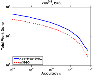
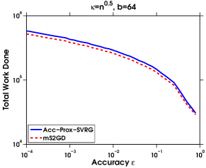
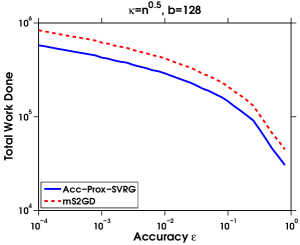
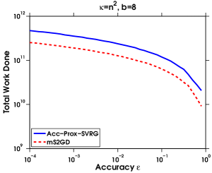
This suggests that acceleration will only be realized when the mini-batch size is large, while for small $b$, Acc-Prox-SVRG achieves the same overall complexity, $\mathcal{O}\left((n+\kappa)\log(1/\epsilon)\right)$, as mS2GD.

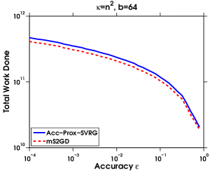
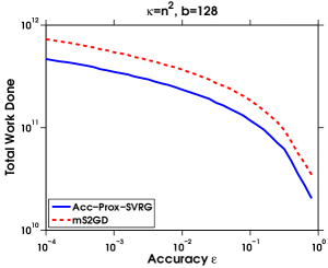
We will now take a closer look at the theoretical results given by Acc-Prox-SVRG and mS2GD, for each $\epsilon\in(0,1)$. In particular, we shall numerically minimize the total work of mS2GD, i.e.,

$$\left(n+2b\lceil m^{b}\rceil\right)\left\lceil\log(1/\epsilon)/\log(1/\rho)\right\rceil,$$

over $\rho\in(0,1)$ and $h$ (compare this with (11)); and compare these results with similar fine-tuned quantities for Acc-Prox-SVRG.

Fig. 1 illustrates these theoretical complexity bounds for both ill-conditioned and well-conditioned data. With small-enough mini-batch size $b$, mS2GD is better than Acc-Prox-SVRG. However, for a large mini-batch size $b$, the situation reverses because of the acceleration inherent in Acc-Prox-SVRG. Plots with $b=64$ illustrate the cases where we cannot observe any differences between the methods.

Note however that accelerated methods are very prone to error accumulation. Moreover, it is not clear that an efficient implementation of Acc-Prox-SVRG is possible for sparse data. As shall show in the next section, mS2GD allows for such an implementation.

V Efficient implementation for sparse data

Let us make the following assumption about the structure of functions $f_{i}$ in (2).

Assumption 3.

The functions $f_{i}$ arise as the composition of a univariate smooth function $\phi_{i}$ and an inner product with a datapoint/example $a_{i}\in\mathbb{R}^{d}$: $f_{i}(x)=\phi(a_{i}^{T}x)$ for $i=1,\dots,n$.

Many functions of common practical interest satisfy this assumption including linear and logistic regression. Very often, especially for large scale datasets, the data are extremely sparse, i.e. the vectors $\{a_{i}\}$ contains many zeros. Let us denote the number of non-zero coordinates of $a_{i}$ by $\omega_{i}=\|a_{i}\|_{0}\leq d$ and the set of indexes corresponding to non-zero coordinates by $\operatorname{support}(a_{i})=\{j:a_{i}^{j}\neq 0\}$, where $a_{i}^{j}$ denotes the $j^{th}$ coordinate of vector $a_{i}$.

Assumption 4.

The regularization function $R$ is separable.

This includes the most commonly used regularization functions as $\frac{\lambda}{2}\|x\|^{2}$ or $\lambda\|x\|_{1}$.

Let us take a brief detour and look at the classical SGD algorithm with $R=0$. The update would be of the form

$$x_{j+1}\leftarrow x_{j}-h\phi^{\prime}_{i}(a_{i}^{T}x_{j})a_{i}=x_{j}-h\nabla f_{i}(x_{j}).$$ (12)

If evaluation of the univariate function $\phi^{\prime}_{i}$ takes $O(1)$ amount of work, the computation of $\nabla f_{i}$ will account for $O(\omega_{i})$ work. Then the update (12) would cost $O(\omega_{i})$ too, which implies that the classical SGD method can naturally benefit from sparsity of data.

Now, let us get back to the Algorithm 1. Even under the sparsity assumption and structural Assumption 3 the Algorithm 1 suggests that each inner iteration will cost $O(\omega+d)\sim O(d)$ because $g_{k}$ is in general fully dense and hence in Step 9 of Algorithm 1 we have to update all $d$ coordinates.

However, in this Section, we will introduce and describe the implementation trick which is based on “lazy/delayed” updates. The main idea of this trick is not to perform Step 9 of Algorithm 1 for all coordinates, but only for coordinates $j\in\cup_{i\in A_{kt}}\operatorname{support}(a_{i})$. The algorithm is described in Algorithm 2.

Algorithm 2 ”Lazy” updates for mS2GD
(these replace steps 6–10 in Algorithm  1)

1:$\chi^{(j)}\leftarrow 0$ for $j=1,2,\dots,d$

2:for $t=0$ to $t_{k}-1$ do

3:     Choose mini-batch $A_{kt}\subseteq[n]$ of size $b$,
.     uniformly at random

4:     for $i\in A_{kt}$ do

5:         for $j\in\operatorname{support}(a_{i})$ do

6:              $y_{k,t}^{j}\leftarrow\operatorname{prox}^{t-\chi^{j}}[y_{k,{\chi^{j}}}^{j},g_{k}^{j},R,h]$

7:              $\chi^{j}\leftarrow t$

8:         end for

9:     end for

10:     ${y}_{k,t+1}\leftarrow{y}_{k,t}-\frac{h}{b}\sum_{i\in A_{kt}}a_{i}(\phi^{\prime}_{i}({y}_{k,t}^{T}a_{i})-\phi^{\prime}_{i}({x}_{k}^{T}a_{i}))$

11:end for

12:for $j=1$ to $d$ do

13:     $y_{k,t_{k}}^{j}\leftarrow\operatorname{prox}^{t_{k}-\chi^{j}}[y_{k,\chi^{j}}^{j},g_{k}^{j},R,h]$

14:end for

To explain the main idea behind the lazy/delayed updates, consider that it happened that during the fist $\tau$ iterations, the value of the fist coordinate in all datapoints which we have used was 0. Then given the values of $y_{k,0}^{1}$ and $g_{k}^{1}$ we can compute the true value of $y_{k,t}^{1}$ easily. We just need to apply the $\operatorname{prox}$ operator $\tau$ times, i.e. $y_{k,\tau}^{1}=\operatorname{prox}^{\tau}_{1}[y_{k,0},g_{k},R,h],$ where the function $\operatorname{prox}^{\tau}_{1}$ is described in Algorithm 3.

Algorithm 3 $\operatorname{prox}^{\tau}_{j}[y,g,R,h]$

$\tilde{y}_{0}=y$

for  $s=1,2,\dots,\tau$ do

     $\tilde{y}_{s}\leftarrow\operatorname{prox}_{hR}(\tilde{y}_{s-1}-hg)$

end for

return $\tilde{y}_{\tau}^{j}$

The vector $\chi$ in Algorithm 2 is enabling us to keep track of the iteration when corresponding coordinate of $y$ was updated for the last time. E.g. if in iteration $t$ we will be updating the $1^{st}$ coordinate for the first time, $\chi^{1}=0$ and after we compute and update the true value of $y^{1}$, its value will be set to $\chi^{1}=t$. Lines 5-8 in Algorithm 2 make sure that the coordinates of $y_{k,t}$ which will be read and used afterwards are up-to-date. At the end of the inner loop, we will updates all coordinates of $y$ to the most recent value (lines 12-14). Therefore, those lines make sure that the $y_{k,t_{k}}$ of Algorithms 1 and 2 will be the same.

However, one could claim that we are not saving any work, as when needed, we still have to compute the proximal operator many times. Although this can be true for a general function $R$, for particular cases, $R(x)=\frac{\lambda}{2}\|x\|^{2}$ and $R(x)=\lambda\|x\|_{1}^{2}$, we provide following Lemmas which give a closed form expressions for the $\operatorname{prox}^{\tau}_{j}$ operator.

Figure 2: Comparison of mS2GD with different mini-batch sizes on rcv1 (left) and astro-ph (right).

Figure 3: Parallelism speedup for rcv1 (left) and astro-ph (right) in theory (unachievable in practice).

Lemma 1 (Proximal Lazy Updates with $\ell_{2}$-Regularizer).

If $R(x)=\frac{\lambda}{2}\|x\|^{2}$ with $\lambda>0$ then

$$\operatorname{prox}_{j}^{\tau}[y,g,R,h]=\beta^{\tau}y^{j}-\tfrac{h\beta}{1-\beta}\left(1-\beta^{\tau}\right)g^{j},$$

where $\beta\stackrel{{\scriptstyle\text{def}}}{{=}}1/(1+\lambda h)$.

Lemma 2 (Proximal Lazy Updates with $\ell_{1}$-Regularizer).

Assume that $R(x)=\lambda\|x\|_{1}$ with $\lambda>0$. Let us define $M$ and $m$ as follows,

$$M=[\lambda+g^{j}]h,\qquad m=-[\lambda-g^{j}]h,$$

and let $[\cdot]_{+}\stackrel{{\scriptstyle\text{def}}}{{=}}\max\{\cdot,0\}$. Then the value of $\operatorname{prox}_{j}^{\tau}[y,g,R,h]$ can be expressed based on one of the 3 situations described below:

1. If $g^{j}\geq\lambda$, then by letting $p\stackrel{{\scriptstyle\text{def}}}{{=}}\left\lfloor\frac{y^{j}}{M}\right\rfloor$, the operator can be defined as

   $$\operatorname{prox}_{j}^{\tau}[y,g,R,h]$$

   $$=\begin{cases}y^{j}-\tau M,&\text{if }p\geq\tau,\\ \min\{y^{j}-[p]_{+}M,m\}-(\tau-[p]_{+})m,&\text{if }p<\tau.\end{cases}$$

2. If $-\lambda<g^{j}<\lambda$, then the operator can be defined as

   $$\operatorname{prox}_{j}^{\tau}[y,g,R,h] =\begin{cases}\max\{y^{j}-\tau M,0\},&\text{if }y^{j}\geq 0,\\ \min\{y^{j}-\tau m,0\},&\text{if }y^{j}<0.\end{cases}$$

3. If $g^{j}\leq-\lambda$, then by letting $q\stackrel{{\scriptstyle\text{def}}}{{=}}\left\lfloor\frac{y^{j}}{m}\right\rfloor$, the operator can be defined as

   $$\operatorname{prox}_{j}^{\tau}[y,g,R,h]$$

   $$=\begin{cases}y^{j}-\tau m,&\text{if }q\geq\tau,\\ \max\{y^{j}-[q]_{+}m,M\}-(\tau-[q]_{+})M,&\text{if }q<\tau.\end{cases}$$

The proofs of Lemmas 1 and 2 are available in APPENDIX C.

Remark: Upon completion of the paper, we learned that similar ideas of lazy updates were proposed in [40] and [41] for online learning and multinomial logistic regression, respectively. However, our method can be seen as a more general result applied to a stochastic gradient method and its variants under Assumptions 3 and 4.

Figure 4: Comparison of several algorithms on four datasets: rcv1 (top left), news20 (top right), covtype (bottom left) and astro-ph (bottom right). We have used mS2GD with $b=8$.

VI Experiments

In this section we perform numerical experiments to illustrate the properties and performance of our algorithm. In Section  VI-A we study the total workload and parallelization speedup of mS2GD as a function of the mini-batch size $b$. In Section VI-B we compare mS2GD with several other algorithms. Finally, in Section VI-C we briefly illustrate that our method can be efficiently applied to a deblurring problem.

In Sections VI-A and VI-B we conduct experiments with $R(x)=\tfrac{\lambda}{2}\|x\|^{2}$ and $F$ of the form (2), where $f_{i}$ is the logistic loss function:

$$f_{i}(x)=\log[1+\exp(-b_{i}a_{i}^{T}x)].$$ (13)

These functions are often used in machine learning, with $(a_{i},b_{i})\in\mathbb{R}^{d}\times\{+1,-1\}$, $i=1,\dots,n$, being a training dataset of example-label pairs. The resulting optimization problem (1)+(2) takes the form

$$\textstyle P(x)=\tfrac{1}{n}\sum_{i=1}^{n}f_{i}(x)+\tfrac{\lambda}{2}\|x\|^{2},$$ (14)

and is used in machine learning for binary classification. In these sections we have performed experiments on four publicly available binary classification datasets, namely rcv1, news20, covtype  and astro-ph .

In the logistic regression problem, the Lipschitz constant of function $\nabla f_{i}$ is equal to $L_{i}=\|a_{i}\|^{2}/4$. Our analysis assumes (Assumption 1) the same constant $L$ for all functions. Hence, we have $L=\max_{i\in[n]}L_{i}$. We set the regularization parameter $\lambda=\frac{1}{n}$ in our experiments, resulting in the problem having the condition number $\kappa=\frac{L}{\mu}=\mathcal{O}(n)$. In Table I we summarize the four datasets, including the sizes $n$, dimensions $d$, their sparsity levels as a proportion of nonzero elements, and the Lipschitz constants $L$.

Dataset	$n$	$d$	Sparsity	$L$
rcv1	20,242	47,236	0.1568%	0.2500
news20	19,996	1,355,191	0.0336%	0.2500
covtype	581,012	54	22.1212%	1.9040
astro-ph	62,369	99,757	0.0767%	0.2500

TABLE I: Summary of datasets used for experiments.

VI-A Speedup of mS2GD

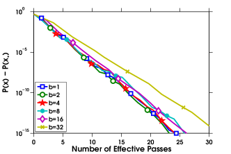
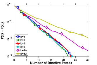
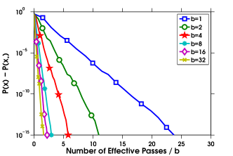
Mini-batches allow mS2GD to be accelerated on a computer with a parallel processor. In Section IV-D, we have shown in that up to some threshold mini-batch size, the total workload of mS2GD remains unchanged. Figure 2 compares the best performance of mS2GD used with various mini-batch sizes on datasets rcv1 and astro-ph. An effective pass (through the data) corresponds to $n$ units of work. Hence, the evaluation of a gradient of $F$ counts as one effective pass. In both cases, by increasing the mini-batch size to $b=2,4,8$, the performance of mS2GD is the same or better than that of S2GD ($b=1$) without any parallelism.

Although for larger mini-batch sizes mS2GD would be obviously worse, the results are still promising with parallelism. In Figure 3,we show the ideal speedup—one that would be achievable if we could always evaluate the $b$ gradients in parallel in exactly the same amount of time as it would take to evaluate a single gradient..

VI-B mS2GD vs other algorithms

In this part, we implemented the following algorithms to conduct a numerical comparison:
1) SGDcon: Proximal stochastic gradient descent method with a constant step-size which gave the best performance in hindsight.
2) SGD+: Proximal stochastic gradient descent with variable step-size $h=h_{0}/(k+1)$, where $k$ is the number of effective passes, and $h_{0}$ is some initial constant step-size.
3) FISTA: Fast iterative shrinkage-thresholding algorithm proposed in [2].
4) SAG: Proximal version of the stochastic average gradient algorithm [4]. Instead of using $h=1/16L$, which is analyzed in the reference, we used a constant step size.
5) S2GD: Semi-stochastic gradient descent method proposed in [7]. We applied proximal setting to the algorithm and used a constant stepsize.
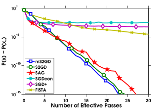
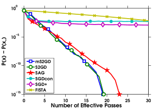
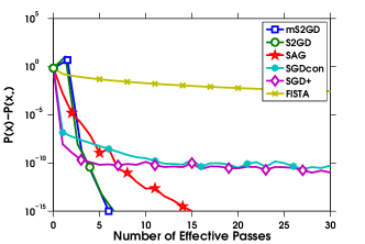
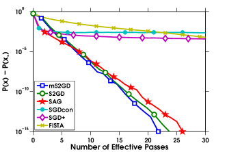
6) mS2GD: mS2GD with mini-batch size $b=8$. Although a safe step-size is given in our theoretical analyses in Theorem 1, we ignored the bound, and used a constant step size.

In all cases, unless otherwise stated, we have used the best constant stepsizes in hindsight.

Figure 4 demonstrates the superiority of mS2GD over other algorithms in the test pool on the four datasets described above. For mS2GD, the best choices of parameters with $b=8$ are given in Table II.

Parameter	rcv1	news20	covtype	astro-ph
$m$	0.11$n$	0.10$n$	0.07$n$	0.08$n$
$h$	$5.5/L$	$6/L$	$350/L$	$6.5/L$

TABLE II: Best choices of parameters in mS2GD.

VI-C Image deblurring

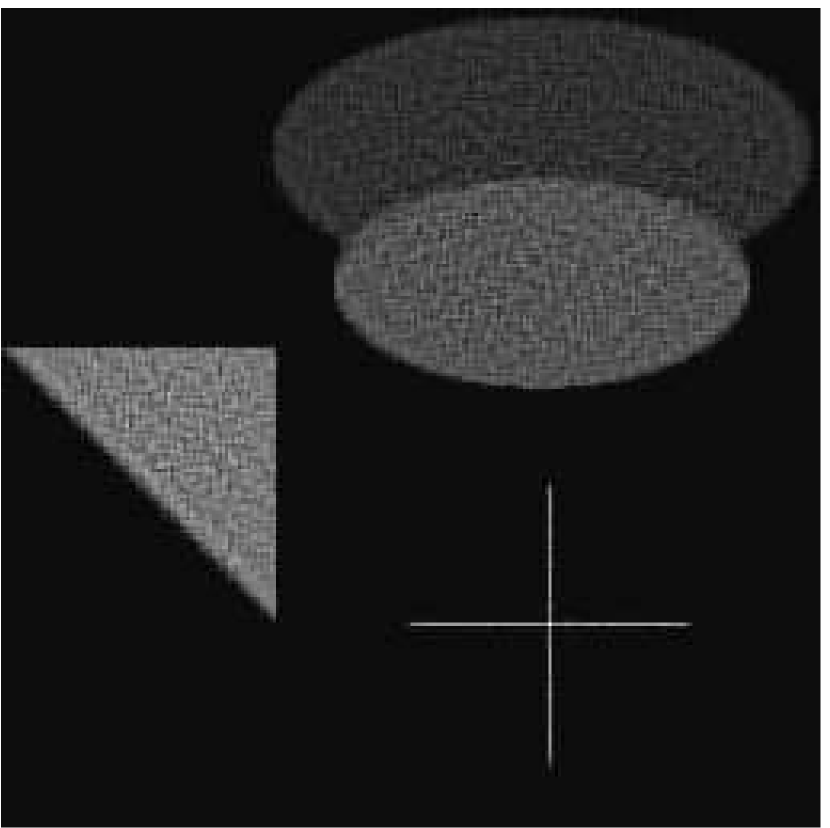
In this section we utilize the Regularization Toolbox [42] We use the blur function available therein to obtain the original image and generate a blurred image (we choose following values of parameters for blur function: $N=256$, band=9, sigma=10). The purpose of the blur function is to generate a test problem with an atmospheric turbulence blur. In addition, an additive Gaussian white noise with stand deviation of $10^{-3}$ is added to the blurred image. This forms our testing image as a vector $b$. The image dimension of the test image is $256\times 256$, which means that $n=d=65,536$. We would not expect our method to work particularly well on this problem since mS2GD works best when $d\ll n$. However, as we shall see, the method’s performance is on a par with the performance of the best methods in our test pool.

Our goal is to reconstruct (de-blur) the original image $x$ by solving a LASSO problem: $\min_{x}\|Ax-b\|_{2}^{2}+\lambda\|x\|_{1}$. We have chosen $\lambda=10^{-4}$. In our implementation, we normalized the objective function by $n$, and hence our objective value being optimized is in fact $\min_{x}\frac{1}{n}\|Ax-b\|_{2}^{2}+\lambda\|x\|_{1}$, where $\lambda=\frac{10^{-4}}{n}$, similarly as was done in [2].

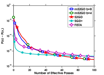
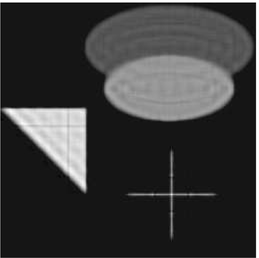
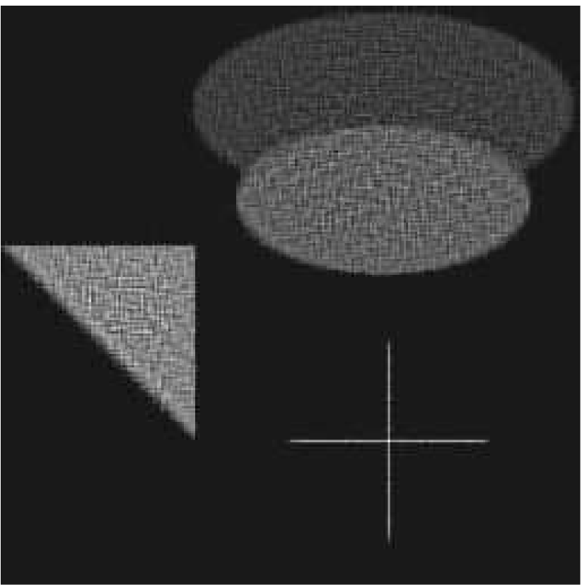
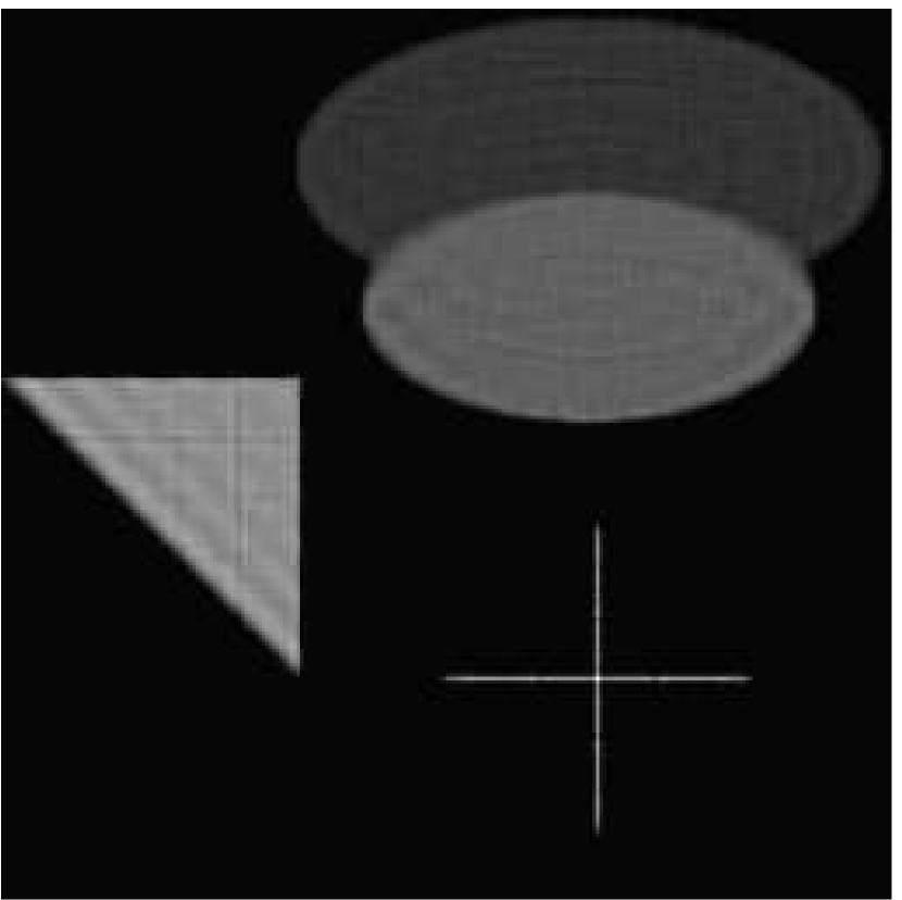
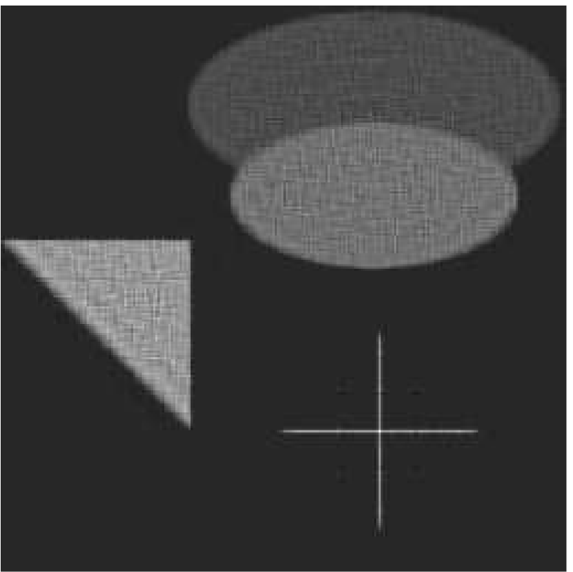
Figure (5) shows the original test image (left) and a blurred image with added Gaussian noise (right). Figure 6 compares the mS2GD algorithm with SGD+, S2GD and FISTA. We run all algorithms for 100 epochs and plot the error. The plot suggests that SGD+ decreases the objective function very rapidly at beginning, but slows down after 10-20 epochs.

Figure 5: Original (left) and blurred & noisy (right) test image.

Figure 6: Comparison of several algorithms for the de-blurring problem.

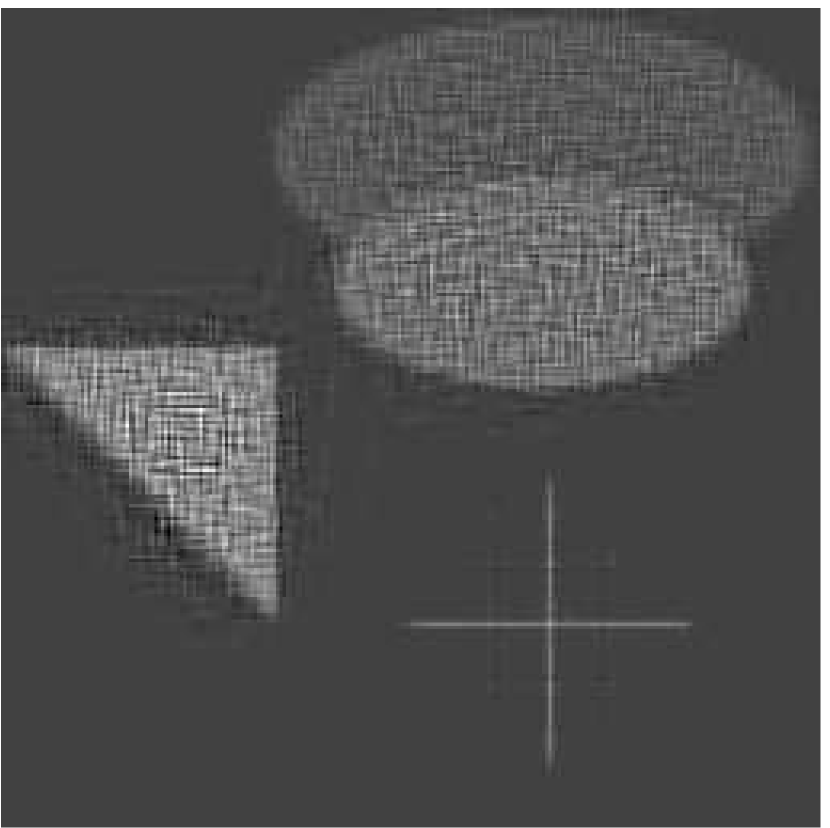
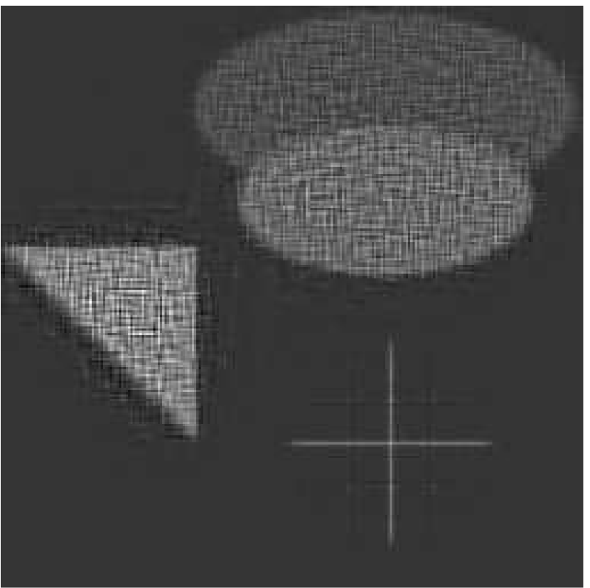
Finally, Fig. 7 shows the reconstructed image after $T=20,60,100$ epochs.

$T=20$
$T=60$
$T=100$

FISTA

SGD+

S2GD

mS2GD $(b=4)$

mS2GD $(b=8)$

Figure 7: Reconstruction of the test image from Figure 5 via FISTA, SGD+, S2GD and mS2GD after $T=20,60,100$ epochs (one epoch corresponds to work equivalent to the computation of one gradient.)

VII Conclusion

We have proposed mS2GD—a mini-batch semi-stochastic gradient method—for minimizing a strongly convex composite function. Such optimization problems arise frequently in inverse problems in signal processing and statistics. Similarly to SAG, SVRG, SDCA and S2GD, our algorithm also outperforms existing deterministic method such as ISTA and FISTA. Moreover, we have shown that the method is by design amenable to a simple parallel implementation. Comparisons to state-of-the-art algorithms suggest that mS2GD, with a small-enough mini-batch size, is competitive in theory and faster in practice than other competing methods even without parallelism. The method can be efficiently implemented for sparse data sets.

Appendix A Technical Results

Lemma 3 (Lemma 3.6 in [35]).

Let $R$ be a closed convex function on $\mathbb{R}^{d}$ and ${x},{y}\in\operatorname{dom}(R)$, then $\|\operatorname{prox}_{R}({x})-\operatorname{prox}_{R}({y})\|\leq\|{x}-{y}\|.$

Note that contractiveness of the proximal operator is a standard result in optimization literature [43, 44].

Lemma 4.

Let $\{\xi_{i}\}_{i=1}^{n}$ be vectors in $\mathbb{R}^{d}$ and $\bar{\xi}\stackrel{{\scriptstyle\text{def}}}{{=}}\frac{1}{n}\sum_{i=1}^{n}\xi_{i}\in\mathbb{R}^{d}$. Let $\hat{S}$ be a random subset of $[n]$ of size $\tau$, chosen uniformly at random from all subsets of this cardinality. Taking expectation with respect to $\hat{S}$, we have

$$\textstyle\operatorname{\mathbf{E}}\left[\left\|\frac{1}{\tau}\sum_{i\in\hat{S}}\xi_{i}-\bar{\xi}\right\|^{2}\right]\leq\frac{1}{n\tau}\frac{n-\tau}{(n-1)}\sum_{i=1}^{n}\left\|\xi_{i}\right\|^{2}.$$ (15)

Following from the proof of Corollary 3.5 in [35], by applying Lemma 4 with $\xi_{i}:=\nabla f_{i}(y_{k,t})-\nabla f_{i}({x}_{k})$, we have the bound for variance as follows.

Theorem 4 (Bounding Variance).

Let $\alpha(b)\stackrel{{\scriptstyle\text{def}}}{{=}}\tfrac{n-b}{b(n-1)}$. Considering the definition of $G_{k,t}$ in Algorithm 1, conditioned on $y_{k,t}$, we have $\operatorname{\mathbf{E}}[G_{k,t}]=\nabla F(y_{k,t})$ and the variance satisfies,

$$\operatorname{\mathbf{E}}\left[\|G_{k,t}-\nabla F(y_{k,t})\|^{2}\right]$$

$$\leq 4L\alpha(b)[P(y_{k,t})-P({x}_{*})+P({x}_{k})-P({x}_{*})].$$ (16)

Appendix B Proofs

B-A Proof of Lemma 4

As in the statement of the lemma, by $\operatorname{\mathbf{E}}[\cdot]$ we denote expectation with respect to the random set $\hat{S}$. First, note that

$$\eta\stackrel{{\scriptstyle\text{def}}}{{=}} \textstyle\operatorname{\mathbf{E}}\left[\left\|\frac{1}{\tau}\sum_{i\in\hat{S}}\xi_{i}-\bar{\xi}\right\|^{2}\right]=\operatorname{\mathbf{E}}\left[\frac{1}{\tau^{2}}\left\|\sum_{i\in\hat{S}}\xi_{i}\right\|^{2}\right]-\|\bar{\xi}\|^{2}$$

$$=\textstyle\frac{1}{\tau^{2}}\operatorname{\mathbf{E}}\left[\sum_{i\in\hat{S}}\sum_{j\in\hat{S}}\xi_{i}^{T}\xi_{j}\right]-\|\bar{\xi}\|^{2}.$$

If we let $C\stackrel{{\scriptstyle\text{def}}}{{=}}\|\bar{\xi}\|^{2}=\frac{1}{n^{2}}\left(\sum_{i,j}\xi_{i}^{T}\xi_{j}\right)$, we can thus write

$$\eta =\textstyle\tfrac{1}{\tau^{2}}\left(\tfrac{\tau(\tau-1)}{n(n-1)}\sum_{i\neq j}\xi_{i}^{T}\xi_{j}+\tfrac{\tau}{n}\sum_{i=1}^{n}\xi_{i}^{T}\xi_{i}\right)-C$$

$$= \textstyle\tfrac{1}{\tau^{2}}\left(\tfrac{\tau(\tau-1)}{n(n-1)}\sum_{i,j}\xi_{i}^{T}\xi_{j}+\left(\tfrac{\tau}{n}-\tfrac{\tau(\tau-1)}{n(n-1)}\right)\sum_{i=1}^{n}\xi_{i}^{T}\xi_{i}\right)-C$$

$$= \textstyle\tfrac{1}{n\tau}\left[-\left(-\tfrac{(\tau-1)}{(n-1)}+\tfrac{\tau}{n}\right)\sum_{i,j}\xi_{i}^{T}\xi_{j}+\tfrac{n-\tau}{n-1}\sum_{i=1}^{n}\xi_{i}^{T}\xi_{i}\right]$$

$$= \textstyle\tfrac{1}{n\tau}\tfrac{n-\tau}{(n-1)}\left[\sum_{i=1}^{n}\xi_{i}^{T}\xi_{i}-\tfrac{1}{n}\sum_{i,j}\xi_{i}^{T}\xi_{j}\right]\leq\textstyle\tfrac{1}{n\tau}\tfrac{n-\tau}{(n-1)}\sum_{i=1}^{n}\left\|\xi_{i}\right\|^{2},$$

where in the last step we have used the bound $\tfrac{1}{n}\sum_{i,j}\xi_{i}^{T}\xi_{j}=n\left\|\sum_{i=1}^{n}\tfrac{1}{n}\xi_{i}\right\|^{2}\geq 0.$

B-B Proof of Theorem 1

The proof is following the steps in [35]. For convenience, let us define the stochastic gradient mapping

$$d_{k,t}=\tfrac{1}{h}(y_{k,t}-y_{k,t+1})=\tfrac{1}{h}(y_{k,t}-\operatorname{prox}_{hR}(y_{k,t}-hG_{k,t})),$$

then the iterate update can be written as $y_{k,t+1}=y_{k,t}-hd_{k,t}.$ Let us estimate the change of $\|y_{k,t+1}-{x}_{*}\|$. It holds that

$$\|y_{k,t+1}-{x}_{*}\|^{2}=\|y_{k,t}-hd_{k,t}-{x}_{*}\|^{2}$$

$$=\|y_{k,t}-{x}_{*}\|^{2}-2hd_{k,t}^{T}(y_{k,t-1}-{x}_{*})+h^{2}\|d_{k,t}\|^{2}.$$ (17)

Applying Lemma 3.7 in [35] (this is why we need to assume that $h\leq 1/L$) with ${x}=y_{k,t}$, $v=G_{k,t}$, ${x}^{+}=y_{k,t+1}$, $g=d_{k,t}$, ${y}={x}_{*}$ and $\Delta=\Delta_{k,t}=G_{k,t}-\nabla F(y_{k,t})$, we get

$$-d_{k,t}^{T}(y_{k,t}-{x}_{*})+\tfrac{h}{2}\|d_{k,t}\|^{2}\leq P({x}_{*})-P(y_{k,t+1})$$

$$-\tfrac{\mu_{F}}{2}\|y_{k,t}-{x}_{*}\|^{2}-\tfrac{\mu_{R}}{2}\|y_{k,t+1}-{x}_{*}\|^{2}-\Delta_{k,t}^{T}(y_{k,t+1}-{x}_{*}),$$ (18)

and therefore,

$$\|y_{k,t+1}-{x}_{*}\|^{2}\overset{\eqref{eq:safwavgfwafa},\eqref{eq:vaawfwavfwafdewafca}}{\leq}2h\left(P({x}_{*})-P(y_{k,t+1})\right.$$

$$\left.-\Delta_{k,t}^{T}(y_{k,t+1}-{x}_{*})\right)+\|y_{k,t}-{x}_{*}\|^{2}$$

$$=\|y_{k,t}-{x}_{*}\|^{2}-2h\Delta_{k,t}^{T}(y_{k,t+1}-{x}_{*})$$

$$-2h[P(y_{k,t+1})-P({x}_{*})].$$ (19)

In order to bound $-\Delta_{k,t}^{T}(y_{k,t+1}-{x}_{*})$, let us define the proximal full gradient update as $\bar{y}_{k,t+1}=\operatorname{prox}_{hR}(y_{k,t}-h\nabla F(y_{k,t})).$ We get

$$-\Delta_{k,t}^{T}(y_{k,t+1}-{x}_{*})$$

$$=-\Delta_{k,t}^{T}(y_{k,t+1}-\bar{y}_{k,t+1})-\Delta_{k,t}^{T}(\bar{y}_{k,t+1}-{x}_{*})$$

$$=-\Delta_{k,t}^{T}(\bar{y}_{k,t+1}-{x}_{*})-\Delta_{k,t}^{T}[\operatorname{prox}_{hR}(y_{k,t}-hG_{k,t})$$

$$\qquad-\operatorname{prox}_{hR}(y_{k,t-1}-h\nabla F(y_{k,t-1}))]$$

Using Cauchy-Schwarz and Lemma 3, we conclude that

$$-\Delta_{k,t}^{T}(y_{k,t+1}-{x}_{*})$$

$$\leq\|\Delta_{k,t}\|\|(y_{k,t}-hG_{k,t})-(y_{k,t}-h\nabla F(y_{k,t}))\|$$

$$\qquad-\Delta_{k,t}^{T}(\bar{y}_{k,t+1}-{x}_{*}),$$

$$=h\|\Delta_{k,t}\|^{2}-\Delta_{k,t}^{T}(\bar{y}_{k,t+1}-{x}_{*}).$$ (20)

Further, we obtain $\|y_{k,t+1}-{x}_{*}\|^{2}\overset{\eqref{eq:asfaevfwavfa},\eqref{eq:safawvfdwavfda}}{\leq}\left\|y_{k,t}-{x}_{*}\right\|^{2}+2h\left(h\|\Delta_{k,t}\|^{2}-\Delta_{k,t}^{T}(\bar{y}_{k,t+1}-{x}_{*})-[P(y_{k,t+1})-P({x}_{*})]\right).$ By taking expectation, conditioned on $y_{k,t}$ we obtain

$$\operatorname{\mathbf{E}}[\|y_{k,t+1}-{x}_{*}\|^{2}]\overset{\eqref{eq:asfaevfwavfa},\eqref{eq:safawvfdwavfda}}{\leq}\left\|y_{k,t}-{x}_{*}\right\|^{2}$$

$$+2h\left(h\operatorname{\mathbf{E}}[\|\Delta_{k,t}\|^{2}]-\operatorname{\mathbf{E}}[P(y_{k,t+1})-P({x}_{*})]\right),$$ (21)

where we have used that $\operatorname{\mathbf{E}}[\Delta_{k,t}]=\operatorname{\mathbf{E}}[G_{k,t}]-\nabla F(y_{k,t})=0$ and hence $\operatorname{\mathbf{E}}[-\Delta_{k,t}^{T}(\bar{y}_{k,t+1}-{x}_{*})]=0$. Now, if we substitute (16) into (21) and decrease index $t$ by 1, we obtain

$$\operatorname{\mathbf{E}}[\|y_{k,t}-{x}_{*}\|^{2}]\overset{\eqref{eq:asfaevfwavfa},\eqref{eq:safawvfdwavfda}}{\leq}\left\|y_{k,t-1}-{x}_{*}\right\|^{2}$$

$$+\theta[P(y_{k,t-1})-P({x}_{*})+P({x}_{k})-P({x}_{*})]$$

$$-2h\operatorname{\mathbf{E}}[P(y_{k,t})-P({x}_{*})],$$ (22)

where

$$\theta\stackrel{{\scriptstyle\text{def}}}{{=}}8Lh^{2}\alpha(b)$$ (23)

and $\alpha(b)=\frac{n-b}{b(n-1)}$. Note that (22) is equivalent to

$$\operatorname{\mathbf{E}}[\|y_{k,t}-{x}_{*}\|^{2}]+2h(\operatorname{\mathbf{E}}[P(y_{k,t})-P({x}_{*})])$$

$$\leq\left\|y_{k,t-1}-{x}_{*}\right\|^{2}$$

$$+\theta\left(P(y_{k,t-1})-P({x}_{*})+P({x}_{k})-P({x}_{*})\right).$$ (24)

Now, by the definition of ${x}_{k}$ in Algorithm 1 we have that

$$\operatorname{\mathbf{E}}[P({x}_{k+1})] =\tfrac{1}{m}\sum_{t=1}^{m}\operatorname{\mathbf{E}}[P(y_{k,t})].$$ (25)

By summing (24) for $1\leq t\leq m$, we get on the left hand side

$$LHS= \sum_{t=1}^{m}\operatorname{\mathbf{E}}[\|y_{k,t}-{x}_{*}\|^{2}]+2h\operatorname{\mathbf{E}}[P(y_{k,t})-P({x}_{*})]$$ (26)

and for the right hand side we have:

$$RHS=\sum_{t=1}^{m}\left\{\operatorname{\mathbf{E}}\|y_{k,t-1}-{x}_{*}\|^{2}+\right.$$

$$\left.\theta\operatorname{\mathbf{E}}[P(y_{k,t-1})-P({x}_{*})+P({x}_{k})-P({x}_{*})]\right\}$$

$$\leq\sum_{t=0}^{m-1}\operatorname{\mathbf{E}}\|y_{k,t}-{x}_{*}\|^{2}+\theta\sum_{t=0}^{m}\operatorname{\mathbf{E}}[P(y_{k,t})-P({x}_{*})]$$

$$+\theta\operatorname{\mathbf{E}}[P({x}_{k})-P({x}_{*})]m.$$ (27)

Combining (26) and (27) and using the fact that $LHS\leq RHS$, we have

$$\operatorname{\mathbf{E}}[\|y_{k,m}-{x}_{*}\|^{2}]+2h\sum_{t=1}^{m}\operatorname{\mathbf{E}}[P(y_{k,t})-P({x}_{*})]$$

$$\leq\operatorname{\mathbf{E}}\|y_{k,0}-{x}_{*}\|^{2}+\theta\operatorname{\mathbf{E}}[P({x}_{k})-P({x}_{*})]m$$

$$+\theta\sum_{t=1}^{m}\operatorname{\mathbf{E}}[P(y_{k,t})-P({x}_{*})]+\theta\operatorname{\mathbf{E}}[P(y_{k,0})-P({x}_{*})].$$

Now, using (25), we obtain

$$\operatorname{\mathbf{E}}[\|y_{k,m}-{x}_{*}\|^{2}]+2hm\operatorname{\mathbf{E}}[P({x}_{k+1})-P({x}_{*})]$$

$$\leq\operatorname{\mathbf{E}}\|y_{k,0}-{x}_{*}\|^{2}+\theta m\operatorname{\mathbf{E}}[P({x}_{k})-P({x}_{*})]$$

$$+\theta m\operatorname{\mathbf{E}}[P({x}_{k+1})-P({x}_{*})]+\theta\operatorname{\mathbf{E}}[P(y_{k,0})-P({x}_{*})].$$ (28)

Strong convexity (7) and optimality of ${x}_{*}$ imply that $0\in\partial P({x}_{*})$, and hence for all ${x}\in\mathbb{R}^{d}$ we have

$$\|{x}-{x}_{*}\|^{2}\leq\tfrac{2}{\mu}[P({x})-P({x}_{*})].$$ (29)

Since $\operatorname{\mathbf{E}}\|{y}_{k,m}-{x}_{*}\|^{2}\geq 0$ and ${y}_{k,0}={x}_{k}$, by combining (29) and (28) we get

$$m(2h-\theta)\operatorname{\mathbf{E}}[P({x}_{k+1})-P({x}_{*})]$$

$$\leq(P({x}_{k})-P({x}_{*}))\left(\tfrac{2}{\mu}+\theta\left(m+1\right)\right).$$

Notice that in view of our assumption on $h$ and (23), we have $2h>\theta$, and hence

$$\operatorname{\mathbf{E}}[P({x}_{k+1})-P({x}_{*})]\leq\rho[P({x}_{k})-P({x}_{*})],$$

where $\rho=\tfrac{2}{m\mu(2h-\theta)}+\tfrac{\theta(m+1)}{m(2h-\theta)}.$ Applying the above linear convergence relation recursively with chained expectations, we finally obtain $\operatorname{\mathbf{E}}[P({x}_{k})-P(x_{*})]\leq\rho^{k}[P({x}_{0})-P(x_{*})].$

B-C Proof of Theorem 2

Clearly, if we choose some value of $h$ then the value of $m$ will be determined from (8) (i.e. we need to choose $m$ such that we will get desired rate). Therefore, $m$ as a function of $h$ obtained from (8) is

$$m(h)=\tfrac{1+4\alpha(b)h^{2}L\mu}{h\mu(\rho-4\alpha(b)hL(\rho+1))}.$$ (30)

Now, we can observe that the nominator is always positive and the denominator is positive only if $\rho>4\alpha(b)hL(\rho+1)$, which implies $\tfrac{1}{4\alpha(b)L}\cdot\tfrac{\rho}{\rho+1}>h$ (note that $\tfrac{\rho}{\rho+1}\in[0,\frac{1}{2}]$). Observe that this condition is stronger than the one in the assumption of Theorem 1. It is easy to verify that

$$\lim_{h\searrow 0}m(h)=+\infty,\qquad\lim_{h\nearrow\frac{1}{4\alpha(b)L}\cdot\frac{\rho}{\rho+1}}m(h)=+\infty.$$

Also note that $m(h)$ is differentiable (and continuous) at any $h\in(0,\frac{1}{4\alpha(b)L}\cdot\frac{\rho}{\rho+1})=:I_{h}$. The derivative of $m$ is given by $m^{\prime}(h)=\tfrac{-\rho+4\alpha(b)hL(2+(2+h\mu)\rho)}{h^{2}\mu(\rho-4\alpha(b)hL(1+\rho))^{2}}.$ Observe that $m^{\prime}(h)$ is defined and continuous for any $h\in I_{h}$. Therefore there have to be some stationary points (and in case that there is just on $I_{h}$) it will be the global minimum on $I_{h}$. The FOC gives

$$\tilde{h}^{b} =\tfrac{-2\alpha(b)L(1+\rho)+\sqrt{\alpha(b)L(\mu\rho^{2}+4\alpha(b)L(1+\rho)^{2})}}{2\alpha(b)L\mu\rho}$$

$$=\sqrt{\tfrac{1}{4\alpha(b)L\mu}+\tfrac{(1+\rho)^{2}}{\mu^{2}\rho^{2}}}-\tfrac{1+\rho}{\mu\rho}.$$ (31)

If this $\tilde{h}^{b}\in I_{h}$ and also $\tilde{h}^{b}\leq\frac{1}{L}$ then this is the optimal choice and plugging (31) into (30) gives us (9).

Claim #1

It always holds that $\tilde{h}^{b}\in I_{h}$. We just need to verify that

$$\sqrt{\tfrac{1}{4\alpha(b)L\mu}+\tfrac{(1+\rho)^{2}}{\mu^{2}\rho^{2}}}-\tfrac{1+\rho}{\mu\rho}<\tfrac{1}{4\alpha(b)L}\cdot\tfrac{\rho}{\rho+1},$$

which is equivalent to $\mu\rho^{2}+4\alpha(b)L(1+\rho)^{2}>2(1+\rho)\sqrt{\alpha(b)L(\mu\rho^{2}+4\alpha(b)L(1+\rho)^{2})}.$ Because both sides are positive, we can square them to obtain the equivalent condition

$$\mu\rho^{2}(\mu\rho^{2}+4\alpha(b)L(1+\rho)^{2})>0.$$

Claim #2

If $\tilde{h}^{b}>\frac{1}{L}$ then $h^{b}_{*}=\frac{1}{L}$. The only detail which needs to be verified is that the denominator of (10) is positive (or equivalently we want to show that $\rho>4\alpha(b)(1+\rho)$. To see that, we need to realize that in that case we have $\tfrac{1}{L}\leq\tilde{h}^{b}\leq\frac{1}{4\alpha(b)L}\cdot\frac{\rho}{\rho+1}$, which implies that $4\alpha(b)(1+\rho)<\rho.$

B-D Proof of Corollary 3

By substituting definition of $\tilde{h}^{b}$ in Theorem 2, we get

$$\tilde{h}^{b}<\tfrac{1}{L}\quad\Longleftrightarrow\quad b<b_{0}\stackrel{{\scriptstyle\text{def}}}{{=}}\tfrac{8\rho n\kappa+8n\kappa+4\rho n}{\rho n\kappa+(7\rho+8)\kappa+4\rho},$$ (32)

where $\kappa=L/\mu$. Hence, it follows that if $b<\lceil b_{0}\rceil$, then $h^{b}=\tilde{h}^{b}$ and $m^{b}$ is defined in (9); otherwise, $h^{b}=\frac{1}{L}$ and $m^{b}$ is defined in (10). Let $e$ be the base of the natural logarithm. By selecting $b_{0}=\frac{8n\kappa+8en\kappa+4n}{n\kappa+(7+8e)\kappa+4}$, choosing mini-batch size $b<\lceil b_{0}\rceil$, and running the inner loop of mS2GD for

$$m_{b}=\left\lceil 8e\alpha(b)\kappa\left(e+1+\sqrt{\tfrac{1}{4\alpha(b)\kappa}+(1+e)^{2}}\right)\right\rceil$$ (33)

iterations with constant stepsize

$$h^{b}=\sqrt{\left(\tfrac{1+e}{\mu}\right)^{2}+\tfrac{1}{4\mu\alpha(b)L}}-\tfrac{1+e}{\mu},$$ (34)

we can achieve a convergence rate

$$\rho \overset{\eqref{s2rho}}{=}\tfrac{1}{m_{b}h^{b}\mu(1-4h^{b}L\alpha(b))}+\tfrac{4h^{b}L\alpha(b)\left(m_{b}+1\right)}{m_{b}(1-4h^{b}L\alpha(b))}\overset{\eqref{eqn:maxiter},\eqref{eqn:stepsizehb}}{=}\tfrac{1}{e}.$$ (35)

Since $k=\left\lceil\log(1/\epsilon)\right\rceil\geq\log(1/\epsilon)$ if and only if $e^{k}\geq 1/\epsilon$ if and only if $e^{-k}\leq\epsilon,$ we can conclude that $\rho^{k}\overset{\eqref{eqn:convergencerate}}{=}(e^{-1})^{k}=e^{-k}\leq\epsilon$. Therefore, running mS2GD for $k$ outer iterations achieves $\epsilon$-accuracy solution defined in (3). Moreover, since in general $\kappa\gg e,n\gg e$, it can be concluded that

$$b_{0}\overset{\eqref{eqn:b0}}{=}\tfrac{8(1+e)n\kappa+4n}{n\kappa+(7+8e)\kappa+4}\approx 8\left(e+1\right)\approx 29.75,$$

then with the definition $\alpha(b)=\frac{(n-b)}{b(n-1)}$, we derive

$$bm_{b}\overset{\eqref{eqn:maxiter}}{=}\left\lceil 8e\kappa\tfrac{(n-b)}{(n-1)}\left(e+1+\sqrt{\tfrac{1}{4\alpha(b)\kappa}+(1+e)^{2}}\right)\right\rceil$$

$$\overset{1\leq b<30}{\leq}\left\lceil 8e\kappa\left((e+1)+\sqrt{\tfrac{b}{4\kappa}+(1+e)^{2}}\right)\right\rceil=\mathcal{O}(\kappa),$$

so from (11), the total complexity can be translated to $\mathcal{O}\left((n+\kappa)\log(1/\epsilon)\right).$ This result shows that we can reach efficient speedup by mini-batching as long as the mini-batch size is smaller than some threshold $b_{0}\approx 29.75$, which finishes the proof for Corollary 3.

Appendix C Proximal lazy updates for $\ell_{1}$ and $\ell_{2}$-regularizers

C-A Proof of Lemma 1

For any $s\in\{1,2,\dots,\tau\}$ we have $\tilde{y}_{s}=\operatorname{prox}_{hR}(\tilde{y}_{s-1}-hg)=\beta(\tilde{y}_{s-1}-hg),$ where $\beta\stackrel{{\scriptstyle\text{def}}}{{=}}1/(1+\lambda h)$. Therefore,

$$\textstyle\tilde{y}_{\tau}=\beta^{\tau}\tilde{y}_{0}-h\left(\sum_{j=1}^{\tau}\beta^{j}\right)g=\beta^{\tau}y-\frac{h\beta}{1-\beta}\left[1-\beta^{\tau}\right]g.$$

C-B Proof of Lemma 2

Proof.

For any $s\in\{1,2,\dots,\tau\}$ and $j\in\{1,2,\dots,d\}$,

$$\tilde{y}_{s}^{j} =\arg\min_{x\in\mathbb{R}}\frac{1}{2}(x-\tilde{y}_{s-1}^{j}+hg^{j})^{2}+\lambda h|x|$$

$$=\begin{cases}\tilde{y}_{s-1}^{j}-(\lambda+g^{j})h,&\text{ if }\tilde{y}_{s-1}^{j}>(\lambda+g^{j})h,\\ \tilde{y}_{s-1}^{j}+(\lambda-g^{j})h,&\text{ if }\tilde{y}_{s-1}^{j}<-(\lambda-g^{j})h,\\ 0,&\text{ otherwise, }\end{cases}$$

$$=\begin{cases}\tilde{y}_{s-1}^{j}-M,&\text{ if }\tilde{y}_{s-1}^{j}>M,\\ \tilde{y}_{s-1}^{j}-m,&\text{ if }\tilde{y}_{s-1}^{j}<m,\\ 0,&\text{ otherwise.}\end{cases}$$

where $M\stackrel{{\scriptstyle\text{def}}}{{=}}(\lambda+g^{j})h$, $m\stackrel{{\scriptstyle\text{def}}}{{=}}-(\lambda-g^{j})h$ and $M-m=2\lambda h>0$. Now, we will distinguish several cases based on $g^{j}$:

1. When $g^{j}\geq\lambda$, then $M>m=-(\lambda-g^{j})h\geq 0$, thus by letting $p=\left\lfloor\frac{y^{j}}{M}\right\rfloor$, we have that: if $y^{j}<m$, then $\tilde{y}^{j}_{\tau}=y^{j}-\tau m;$ if $m\leq y^{j}<M$, then $\tilde{y}_{\tau}^{j}=-(\tau-1)m;$ and if $y^{j}\geq M$, then

   $$\tilde{y}_{\tau}^{j} =\begin{cases}y^{j}-\tau M,&\text{ if }\tau\leq p,\\ y^{j}-pM-(\tau-p)m,&\text{ if }\tau>p\text{ \& }y^{j}-pM<m,\\ -(\tau-p-1)m,&\text{ if }\tau>p\text{ \& }y^{j}-pM\geq m,\end{cases}$$

   $$=\begin{cases}y^{j}-\tau M,&\text{ if }\tau\leq p,\\ \min\{y^{j}-pM,m\}-(\tau-p)m,&\text{ if }\tau>p.\end{cases}$$

2. When $-\lambda<g^{j}<\lambda$, then $M=(\lambda+g^{j})h>0,m=-(\lambda-g^{j})h<0$, thus we have that

   $$\tilde{y}_{\tau}^{j}=\begin{cases}\max\{y^{j}-\tau M,0\},&\text{ if }y^{j}\geq 0,\\ \min\{y^{j}-\tau m,0\},&\text{ if }y^{j}<0.\end{cases}$$

3. When $g^{j}\leq-\lambda$, then $m<M=(\lambda+g^{j})h\leq 0$, thus by letting $q=\left\lfloor\frac{y^{j}}{m}\right\rfloor$, we have that: if $y^{j}\leq m$, then

   $$\tilde{y}_{\tau}^{j} =\begin{cases}y^{j}-\tau m,&\text{ if }\tau\leq q,\\ y^{j}-pm-(\tau-q)M,&\text{ if }\tau>q\text{ \& }y^{j}-qm>M,\\ -(\tau-q-1)M,&\text{ if }\tau>q\text{ \& }y^{j}-qm\leq M,\end{cases}$$

   $$=\begin{cases}y^{j}-\tau m,&\text{ if }\tau\leq q,\\ \max\{y^{j}-qm,M\}-(\tau-q)M,&\text{ if }\tau>q;\end{cases}$$

   if $m<y^{j}\leq M$, then $\tilde{y}_{\tau}^{j}=-(\tau-1)M;$ if $y^{j}>M$, then $\tilde{y}_{\tau}^{j}=y^{j}-\tau M.$

Now, we will perform a few simplifications: Case (1). When $y^{j}<M$, we can conclude that $\tilde{y}_{\tau}^{j}=\min\{y^{j},m\}-\tau m.$ Moreover, since the following equivalences hold if $g^{j}\geq\lambda$: $y^{j}\geq M\ \Leftrightarrow\ \tfrac{y^{j}}{M}\geq 1\ \Leftrightarrow\ p\geq 1$, and $y^{j}<M\ \Leftrightarrow\ \tfrac{y^{j}}{M}<1\ \Leftrightarrow\ p\leq 0$, the situation simplifies to

$$\tilde{y}_{\tau}^{j} \quad=\begin{cases}y^{j}-\tau M,&\text{if }p\geq\tau,\\ \min\{y^{j}-pM,m\}-(\tau-p)m,&\text{if }1\leq p<\tau,\\ \min\{y^{j},m\}-\tau m,&\text{if }p\leq 0,\end{cases}$$

$$\quad=\begin{cases}y^{j}-\tau M,&\text{if }p\geq\tau,\\ \min\{y^{j}-[p]_{+}M,m\}-(\tau-[p]_{+})m,&\text{if }p<\tau,\end{cases}$$

where $[\cdot]_{+}\stackrel{{\scriptstyle\text{def}}}{{=}}\max\{\cdot,0\}$. For Case (3), when $y^{j}>m$, we can conclude that $\tilde{y}_{\tau}^{j}=\max\{y^{j},M\}-\tau M,$ and in addition, the following equivalences hold when $g^{j}\leq-\lambda$:

$$y^{j}\leq m\ \Leftrightarrow\ \tfrac{y^{j}}{m}\geq 1\ \Leftrightarrow\ q\geq 1,$$

$$y^{j}>m\ \Leftrightarrow\ \tfrac{y^{j}}{m}<1\ \Leftrightarrow\ q\leq 0,$$

which summarizes the situation as follows:

$$\tilde{y}_{\tau}^{j} \quad=\begin{cases}y^{j}-\tau m,&\text{if }q\geq\tau,\\ \max\{y^{j}-qm,M\}-(\tau-q)M,&\text{if }1\leq q<\tau,\\ \max\{y^{j},M\}-\tau M,&\text{if }q\leq 0,\end{cases}$$

$$\quad=\begin{cases}y^{j}-\tau m,&\text{if }q\geq\tau,\\ \max\{y^{j}-[q]_{+}m,M\}-(\tau-[q]_{+})M,&\text{if }q<\tau.\end{cases}\qed$$

References

- [1] Y. Nesterov, “Gradient methods for minimizing composite objective function,” CORE Discussion Papers, 2007.
- [2] A. Beck and M. Teboulle, “A fast iterative shrinkage-thresholding algorithm for linear inverse problems,” SIAM J. Imaging Sciences, vol. 2, no. 1, pp. 183–202, 2009.
- [3] H. Robbins and S. Monro, “A stochastic approximation method,” The Annals of Mathematical Statistics, vol. 22, no. 3, pp. 400–407, 1951.
- [4] N. Le Roux, M. Schmidt, and F. Bach, “A stochastic gradient method with an exponential convergence rate for finite training sets,” NIPS, pp. 2672–2680, 2012.
- [5] S. Shalev-Shwartz and T. Zhang, “Stochastic dual coordinate ascent methods for regularized loss,” JMLR, vol. 14, no. 1, pp. 567–599, 2013.
- [6] R. Johnson and T. Zhang, “Accelerating stochastic gradient descent using predictive variance reduction,” NIPS, pp. 315–323, 2013.
- [7] J. Konečný and P. Richtárik, “Semi-stochastic gradient descent methods,” arXiv:1312.1666, 2013.
- [8] Y. Nesterov, “Efficiency of coordinate descent methods on huge-scale optimization problems,” SIAM J. Optimization, vol. 22, pp. 341–362, 2012.
- [9] P. Richtárik and M. Takáč, “Iteration complexity of randomized block-coordinate descent methods for minimizing a composite function,” Mathematical Programming, vol. 144, no. 1-2, pp. 1–38, 2014.
- [10] P. Richtárik and M. Takáč, “Parallel coordinate descent methods for big data optimization,” Mathematical Programming, Series A, pp. 1–52, 2015.
- [11] I. Necoara and A. Patrascu, “A random coordinate descent algorithm for optimization problems with composite objective function and linear coupled constraints,” Comp. Optimization and Applications, vol. 57, no. 2, pp. 307–337, 2014.
- [12] O. Fercoq and P. Richtárik, “Accelerated, parallel and proximal coordinate descent,” arXiv:1312.5799, 2013.
- [13] J. Mareček, P. Richtárik, and M. Takáč, “Distributed block coordinate descent for minimizing partially separable functions,” arXiv:1406.0238, 2014.
- [14] I. Necoara and D. Clipici, “Distributed coordinate descent methods for composite minimization,” arXiv:1312.5302, 2013.
- [15] P. Richtárik and M. Takáč, “Distributed coordinate descent method for learning with big data,” arXiv:1310.2059, 2013.
- [16] O. Fercoq, Z. Qu, P. Richtárik, and M. Takáč, “Fast distributed coordinate descent for non-strongly convex losses,” in IEEE Workshop on Machine Learning for Signal Processing, 2014.
- [17] Z. Qu and P. Richtárik, “Coordinate descent with arbitrary sampling I: algorithms and complexity,” arXiv:1412.8060, 2014.
- [18] P. L. Combettes and J.-C. Pesquet, “Stochastic quasi-fejér block-coordinate fixed point iterations with random sweeping,” SIAM Journal on Optimization, vol. 25, no. 2, pp. 1221–1248, 2015.
- [19] T. Zhang, “Solving large scale linear prediction using stochastic gradient descent algorithms,” in ICML, 2004.
- [20] C. Ma, V. Smith, M. Jaggi, M. I. Jordan, P. Richtárik, and M. Takáč, “Adding vs. averaging in distributed primal-dual optimization,” ICML, pp. 1973–1982, 2015.
- [21] M. Jaggi, V. Smith, M. Takáč, J. Terhorst, T. Hofmann, and M. I. Jordan, “Communication-efficient distributed dual coordinate ascent,” NIPS, pp. 3068–3076, 2014.
- [22] M. Takáč, A. S. Bijral, P. Richtárik, and N. Srebro, “Mini-batch primal and dual methods for SVMs,” ICML, pp. 1022–1030, 2013.
- [23] A. Nitanda, “Stochastic proximal gradient descent with acceleration techniques,” NIPS, pp. 1574–1582, 2014.
- [24] L. Rosasco, S. Villa, and B. C. Vũ, “Convergence of stochastic proximal gradient algorithm,” arXiv:1403.5074, 2014.
- [25] T. Strohmer and R. Vershynin, “A Randomized Kaczmarz Algorithm with Exponential Convergence,” Journal of Fourier Analysis and Applications, vol. 15, no. 2, pp. 262–278, 2009.
- [26] D. Needell, “Randomized Kaczmarz solver for noisy linear systems,” BIT, vol. 50, no. 2, pp. 395–403, 2010.
- [27] A. Zouzias and N. Freris, “Randomized Extended Kaczmarz for Solving Least-Squares,” arXiv preprint arXiv:1205.5770, p. 19, 2012. [Online]. Available: http://arxiv.org/abs/1205.5770
- [28] A. Ma, D. Needell, A. Ramdas, and N. A. Mar, “Convergence Properties of the Randomized Extended Gauss-Seidel and Kaczmarz methods,” arXiv:1503.08235, pp. 1–16, 2015.
- [29] P. Oswald and W. Zhou, “Convergence analysis for Kaczmarz-type methods in a Hilbert space framework,” Linear Algebra and its Applications, vol. 478, pp. 131–161, 2015. [Online]. Available: http://linkinghub.elsevier.com/retrieve/pii/S0024379515001925
- [30] R. Needell, Deanna and Srebro, Nathan and Ward, “Stochastic Gradient Descent, Weighted Sampling, and the Randomized Kaczmarz Algorithm,” Mathematical Programming, 2015.
- [31] R. M. Gower and P. Richtárik, “Randomized Iterative Methods for Linear Systems,” arXiv:1506.03296, 2015.
- [32] D. Leventhal and A. S. Lewis, “Randomized Methods for Linear Constraints: Convergence Rates and Conditioning,” p. 22, 2008. [Online]. Available: http://arxiv.org/abs/0806.3015
- [33] D. a. Spielman and S.-H. Teng, “Nearly-Linear Time Algorithms for Preconditioning and Solving Symmetric, Diagonally Dominant Linear Systems,” vol. 35, no. 3, pp. 835–885, 2006. [Online]. Available: http://arxiv.org/abs/cs/0607105
- [34] Z. Qu, P. Richtárik, and T. Zhang, “Randomized dual coordinate ascent with arbitrary sampling,” in NIPS, 2015.
- [35] L. Xiao and T. Zhang, “A proximal stochastic gradient method with progressive variance reduction,” SIAM Journal on Optimization, vol. 24, no. 4, pp. 2057–2075, 2014.
- [36] P. L. Combettes and J.-C. Pesquet, “Proximal splitting methods in signal processing,” in Fixed-Point Algorithms for Inverse Problems in Science and Engineering. Springer, 2011, vol. 49, pp. 185–212.
- [37] N. Parikh and S. Boyd, “Proximal algorithms,” Foundations and Trends in Opimization, vol. 1, no. 3, pp. 127–239, 2014.
- [38] J. Konečný, J. Liu, P. Richtárik, and M. Takáč, “Mini-batch semi-stochastic gradient descent in the proximal setting,” arXiv:1504.04407, 2015.
- [39] Y. Nesterov, Introductory Lectures on Convex Optimization: A Basic Course. Kluwer, Boston, 2004.
- [40] J. Langford, L. Li, and T. Zhang, “Sparse online learning via truncated gradient,” Journal of Machine Learning Research, vol. 10, pp. 777–801, 2009.
- [41] B. Carpenter, “Lazy sparse stochastic gradient descent for regularized multinomial logistic regression,” Technical Report, April 2008.
- [42] P. C. Hansen, “Regularization tools version 4.0 for matlab 7.3,” Numerical algorithms, vol. 46, no. 2, pp. 189–194, 2007.
- [43] J. J. Moreau, “Fonctions convexes duales et points proximaux dans un espace hilbertien,” in Reports of the Paris Academy of Sciences, ser. A, vol. 255, 1962, pp. 2897–2899.
- [44] R. T. Rockafellar, Convex Analysis. Princeton University Press, 1970.