Signatures of Horndeski gravity on the Dark Matter Bispectrum

Abstract

We present a detailed study of second-order matter perturbations for the general Horndeski class of models. Being the most general scalar-tensor theory having second-order equations of motion, it includes many known gravity and dark energy theories and General Relativity with a cosmological constant as a specific case. This enables us to estimate the leading order dark matter bispectrum generated at late-times by gravitational instability. We parametrize the evolution of the first and second-order equations of motion as proposed by Bellini and Sawicki (2014), where the free functions of the theory are assumed to be proportional to the dark energy density. We show that it is unnatural to have large $\gtrsim 10\%$ ($\gtrsim 1\%$) deviations of the bispectrum introducing even larger $\sim 30\%$ ($\sim 5\%$) deviations in the linear growth rate. Considering that measurements of the linear growth rate have much higher signal-to-noise than bispectrum measurements, this indicates that for Horndeski models which reproduce the expansion history and the linear growth rate as predicted by GR the dark matter bispectrum kernel can be effectively modelled as the standard GR one. On the other hand, an observation of a large bispectrum deviation that can not be explained in terms of bias would imply either that the evolution of perturbations is strongly different than the evolution predicted by GR or that the theory of gravity is exotic (e.g., breaks the weak equivalence principle) and/or fine-tuned.

1 Introduction

One of the most challenging problems in modern cosmology is to understand the nature of the accelerated expansion of the Universe at late-times [1, 2]. The simplest model that explains this behaviour is the $\Lambda$-cold dark matter one ($\Lambda\textrm{CDM}$), where gravity is described by General Relativity (GR) at all scales and the the cosmological constant $\Lambda$ is used in order to have acceleration on cosmological scales. It is a simple model, with a minimal number of parameters that fits exceptionally well a suite of observations ranging from the early Universe to today and over 4 order of magnitude in scale [3, 4]. However, the value of $\Lambda$ appears to be too small to be explained by fundamental physics (e.g., [5]).

One popular alternative is to add a scalar degree of freedom to the Einstein equations, either by acting as an additional and exotic fluid of the system (as for Dark Energy (DE) models), or by modifying directly the laws of gravity (as for Modified Gravity (MG) models). In this paper we focus on the Horndeski theory introduced in [6, 7, 8]. The action reads

$$S=\int\mathrm{d}^{4}x\,\sqrt{-g}\left[\sum_{i=2}^{5}{\cal L}_{i}\,+\mathcal{L}_{\text{m}}[g_{\mu\nu}]\right]\,,$$ (1.1)

where $g_{\mu\nu}$ is the metric, $\mathcal{L}_{\textrm{m}}$ is the matter lagrangian, which contains just one single fluid composed by Dark Matter (DM) and baryonic matter, and $\mathcal{L}_{i}$ are

$${\cal L}_{2} = K(\phi,\,X)\,,$$ (1.2)

$${\cal L}_{3} = -G_{3}(\phi,\,X)\Box\phi\,,$$ (1.3)

$${\cal L}_{4} = G_{4}(\phi,\,X)R+G_{4X}(\phi,\,X)\left[\left(\Box\phi\right)^{2}-\phi_{;\mu\nu}\phi^{;\mu\nu}\right]\,,$$ (1.4)

$${\cal L}_{5} = G_{5}(\phi,\,X)G_{\mu\nu}\phi^{;\mu\nu}-\frac{1}{6}G_{5X}(\phi,\,X)\left[\left(\Box\phi\right)^{3}+2{\phi_{;\mu}}^{\nu}{\phi_{;\nu}}^{\alpha}{\phi_{;\alpha}}^{\mu}-3\phi_{;\mu\nu}\phi^{;\mu\nu}\Box\phi\right]\,.$$ (1.5)

Here, $K$, $G_{3}$, $G_{4}$ and $G_{5}$ are arbitrary functions of the scalar field $\phi$ and its canonical kinetic term $X=-\phi^{;\mu}\phi_{;\mu}/2$. The subscript $X$ represents a derivative with respect to (w.r.t.) $X$, while a subscript $\phi$ would denote a derivative w.r.t. the scalar field $\phi$. The action, Eq. (1.1), is the most general action for a single scalar field that has second-order equations of motion on any background and satisfies the weak equivalence principle, i.e., all matter species are coupled minimally and universally to the metric $g_{\mu\nu}$. It encompasses many of the classical DE/MG models studied to explain the late-time cosmic acceleration: quintessence [9, 10], kinetic gravity braiding [11, 12, 13], galileons [14, 15], $f\left(R\right)$ [16]. We must note that with the Horndeski lagrangian it is not possible to describe models which break the weak equivalence principle, such as coupled quintessence [17] and non-universal disformal couplings [18, 19, 20], or Lorentz-invariance-violating models (e.g. Hořava-Lifshitz gravity [21, 22]), or beyond Horndeski theories [23, 24].

Measurements of the expansion history of the Universe are in excellent agreement with $\Lambda\textrm{CDM}$, e.g. [4]. Then, it is justified to assume it as our fiducial model for the background evolution. However, the same behaviour could be obtained assuming a particular DE/MG model with the requirement that the equation of state of the new degree of freedom is $w\left(t\right)\equiv\frac{p\left(t\right)}{\rho\left(t\right)}\thickapprox-1$, where $\rho\left(t\right)$ and $p\left(t\right)$ are the background energy density and pressure of the DE/MG fluid respectively.

It is important to look at the growth of cosmological perturbations via gravitational instability as traced by the Large Scale Structure (LSS) of the Universe to learn about the nature of the cosmic acceleration. Indeed in $\Lambda\textrm{CDM}$, and in minimally coupled quintessence models, once the expansion history is given, the growth of structures is fully determined. This one-to-one correspondence is broken by the additional degree of freedom if we use a generic sub-class of the Horndeski action, Eq. (1.1). As explained in greater detail in the following section, it is therefore important to have a description that separates the expansion history from the evolution of the perturbations. This result can be achieved by using an Effective Field Theory approach, which has been developed for Horndeski models in [25, 26, 27, 28, 29, 30, 31].

In this paper we look at the evolution of matter perturbations at first and second orders by using the general Horndeski action Eq. (1.1). The first statistics of interest is the Power Spectrum (PS) $P\left(t,k\right)$ defined as

$$\left\langle\delta\left(t,\vec{k}_{1}\right)\delta\left(t,\vec{k}_{2}\right)\right\rangle\equiv\left(2\pi\right)^{3}\delta^{(3)}\left(\vec{k}_{1}+\vec{k}_{2}\right)P\left(t,k_{1}\right)\,,$$ (1.6)

where $\delta\left(t,\vec{k}\right)\equiv\frac{\delta\rho\left(t,\vec{k}\right)}{\rho\left(t\right)}$ is the matter density contrast, $\delta^{(3)}$ is the 3-dimensional Dirac delta, and $\left\langle\ldots\right\rangle$ indicates the ensemble averaging over the possible configurations of the Universe. The PS encodes all the statistical information of a Gaussian random field. However, due to gravitational instability, which amplifies the initial small fluctuations, the late Universe is highly non-Gaussian. The lowest order statistics sensitive to the non-linearities is the bispectrum $B\left(t,\vec{k}_{1},\vec{k}_{2},\vec{k}_{3}\right)$, defined as

$$\left\langle\delta\left(t,\vec{k}_{1}\right)\delta\left(t,\vec{k}_{2}\right)\delta\left(t,\vec{k}_{3}\right)\right\rangle\equiv\left(2\pi\right)^{3}\delta^{(3)}\left(\vec{k}_{1}+\vec{k}_{2}+\vec{k}_{3}\right)B\left(t,\vec{k}_{1},\vec{k}_{2},\vec{k}_{3}\right)\,,$$ (1.7)

where the Dirac delta imposes that only closed triangle configurations are to be considered.

In GR the expansion history of the Universe determines the growth of the perturbations at all orders. Therefore, linear and non linear growth histories do not add qualitatively new information (beside shrinking the statistical error-bars). In this paper we want to show in which cases the DM bispectrum carries significantly new information about the growth of structures that is not included in the linear-order growth. With the data coming from current and forthcoming Large Scale Structure (LSS) surveys, such as BOSS [32], WiggleZ [33], DES [34] or Euclid [35], it will be possible to measure the PS and the bispectrum with unprecedented statistical precision ($\sim 1\%$). The PS is a well known tried and tested statistical tool, a work-horse of any statistical analysis of LSS, which is extremely high signal to noise, and with well understood statistical properties. The linear growth rate can be measured in several independent ways (e.g., weak lensing, redshift space distortions etc.). On the other hand (mildly) non-linear growth is much harder to measure. The most widespread tool is the bispectrum, but it has much lower signal to noise and the information is spread out over several configurations. It is complicated to model and time consuming even in a standard GR-$\Lambda$CDM model (eg. [36, 37]). Then, we want to know to what extent the modelling developed for this “fiducial” case (i.e. GR-$\Lambda$CDM) is more general and can be applied more widely.

The general result for the leading order DM bispectrum assuming Gaussian initial conditions reads (e.g., see [38] for a review)

$$B\left(t,\vec{k}_{1},\vec{k}_{2},\vec{k}_{3}\right)=F_{2}\left(t,\vec{k}_{1},\vec{k}_{2}\right)\,P\left(t,k_{1}\right)\,P\left(t,k_{2}\right)+cyc.,$$ (1.8)

where $cyc.$ contains the possible permutations w.r.t $\vec{k}_{i}$ and $F_{2}$ is a model dependent kernel which was derived for Horndeski models in [39]. We shall show the expression for $F_{2}$ in the next section. Here, it is important to note that the functional form of the bispectrum in terms of the kernel and the linear PS is identical to the standard one. As a result of Eq. (1.8), the tree-level DM bispectrum can be separated in terms of linear quantities, i.e. $P\left(t,\vec{k}\right)$, and second-order quantities, i.e. $F_{2}\left(t,\vec{k}_{1},\vec{k}_{2}\right)$. The DM bispectrum has been investigated using second-order perturbation theory or simulations in simple DE/MG theories as Brans-Dicke/$f(R)$ or cubic galileon [40, 41, 42, 43, 44]. The result is that, in these Horndeski sub-models, the DM bispectrum kernel appears to be close to the standard one within deviations at the percent level, and then it can be approximated as $F_{2}\simeq F_{2\textrm{GR}}$. The main goal of this paper is to investigate if it is possible to generalise this approximation for a wider class of Horndeski-type DE/MG models. In these cases, it would be possible to avoid the second-order analysis, and concentrate just on the evolution of linear perturbations by applying directly the bispectrum constraints obtained assuming $\Lambda$CDM/GR e.g., [36, 37].

The paper is organised as follows. In Section 2 we describe the approach we used and show the main equations, while Appendix A is reserved to useful formulas that are too long to fit in the main text. In Section 3 we present and discuss the main results, and in Section 4 we draw our conclusions.

2 Approach

We assume that the Universe at large enough scales is well described by small perturbations on top of a flat Friedmann-Robertson-Walker (FRW) metric. We consider scalar perturbations in the Newtonian gauge, and adopt the notation of [45]. Then, up to second order the line element reads

$$\mathrm{d}s^{2}=-(1+2\Psi+\Psi^{(2)})\mathrm{d}t^{2}+a^{2}(t)(1-2\Phi-\Phi^{(2)})\mathrm{d}\boldsymbol{x}^{2}\,,$$ (2.1)

where for brevity we have neglected the superscript $(1)$ for linear perturbations. Here $\Psi$ and $\Phi$ are the metric perturbations and in this gauge they can be interpreted as the gauge invariant Bardeen’s potentials [46]. The perturbation of the scalar field is rewritten as $v_{X}\equiv-\delta\phi/\dot{\phi}$, where $\phi$ and $\delta\phi$ are the background and the perturbation of the scalar in Eq. (1.1) respectively. In the following we will show the equations for the metric perturbations, after having decoupled them from the scalar field perturbations.

In [31], see also [27, 28, 26] for an equivalent approach, the authors describe the evolution of linear perturbations in general scalar-tensor theories belonging to the Horndeski class of models, Eq. (1.1). The idea is to identify the minimum number of operators that fully specify the linear evolution of those models (see [31] for details). These operators are independent of each other, i.e., they can be parametrized independently. One of the advantages of this description is that it separates the effects of the background expansion from the effects of the perturbations. Then, the total amount of cosmological information can be compressed into five functions of time plus one constant, namely

$$\{\Omega_{\textrm{m}0},H\left(t\right),\alpha_{\textrm{K}}\left(t\right),\alpha_{\textrm{B}}\left(t\right),\alpha_{\textrm{M}}\left(t\right),\alpha_{\textrm{T}}\left(t\right)\}\,,$$ (2.2)

where $\Omega_{\textrm{m}0}$ is the value of the matter density fraction today, $H\left(t\right)$ is the Hubble function and $\alpha_{i}\left(t\right)$ represent the linear freedom of the Horndeski class of models. $\alpha_{\textrm{K}}$, the kineticity, is the most standard kinetic term present in simple DE models as quintessence or k-essence. $\alpha_{\textrm{B}}$ is called braiding, it represents a mixing between the kinetic terms of the metric and the scalar. $\alpha_{\textrm{M}}$, the Planck mass run rate, describes systems in which the Planck mass is varying with time. $\alpha_{\textrm{T}}$ is the tensor speed excess, and it directly modifies the speed of tensors. Both $\alpha_{\textrm{M}}$ and $\alpha_{\textrm{T}}$ produce anisotropic stress between the gravitational potentials $\Psi$ and $\Phi$, and they are signatures of modifications in the evolution of the gravitational waves [47]. Generalizing the results of [31] to second-order in perturbation theory we find four other functions of time which are free to vary in the general Horndeski theory. However, for our purposes we just need two of them, since the other two appear in front of terms that are sub-dominant on sub-horizon scales ($k^{2}\gg a^{2}H^{2}$). Then, the total freedom one can have is represented by

$$\{\Omega_{\textrm{m}0},H\left(t\right),\alpha_{\textrm{K}}\left(t\right),\alpha_{\textrm{B}}\left(t\right),\alpha_{\textrm{M}}\left(t\right),\alpha_{\textrm{T}}\left(t\right),\alpha_{5}\left(t\right),\alpha_{4}\left(t\right)\}\,,$$ (2.3)

where the new functions $\alpha_{5}$ and $\alpha_{4}$ represent the second-order freedom of this theory and are defined in Appendix A. From their definitions, $\alpha_{5}$ and $\alpha_{4}$ can be considered as second-order corrections to $\alpha_{\textrm{M}}$ and $\alpha_{\textrm{T}}$, then we can expect that realistic DE/MG theories will have

$$\left|\alpha_{5},\alpha_{4}\right|\lesssim\left|\alpha_{\textrm{M}},\alpha_{\textrm{T}}\right|\lesssim{\cal O}(1)\,.$$ (2.4)

Models that do not satisfy the second inequality have a strong non-minimal coupling, and they are expected to drastically modify the evolution of first-order scalar and tensor perturbations. Then, they can be excluded by observations that rely on linear theory, without the need of second-order analysis. The first inequality in Eq. (2.4) describes the fact that $\alpha_{5}$ and $\alpha_{4}$ are built with the same Horndeski functions as $\alpha_{\textrm{M}}$ and $\alpha_{\textrm{T}}$, i.e., $G_{4}$ and $G_{5}$ (see Eq. (A.1-A.2) and Ref. [31] for comparison). In principle it is possible to create a model in which the second-order functions are larger than the first-order ones, but it would require fine tuning. We consider Eq. (2.4) as a naturalness condition, which we will however not impose a priori. While our analysis below is general and does not assume this hierarchy, it is reasonable to concentrate attention on the ”natural” regime of Eq. (2.4).

As specified above, with this approach we separate the contribution of the background from the perturbations. Indeed, the $\alpha_{i}$ functions are constructed to be independent form the background in the general Horndeski class of models. Then, we can assume a flat $\Lambda\textrm{CDM}$ cosmology for the evolution of $H\left(t\right)$ and fix $\Omega_{\textrm{m}0}=0.31$ [4], this being our fiducial model. The Friedmann and the conservation equations read

$$2\dot{H}=-3H^{2}\tilde{\Omega}_{\text{m}}$$ (2.5)

$$\dot{\tilde{\Omega}}_{\text{m}}+3H\tilde{\Omega}_{\text{m}}\left(1-\tilde{\Omega}_{\text{m}}\right)=-H\tilde{\Omega}_{\text{m}}\alpha_{\textrm{M}}\,,$$ (2.6)

where $\tilde{\Omega}_{\textrm{m}}\equiv\frac{\rho_{\textrm{m}}}{3M_{*}^{2}H^{2}}$ is the DM fractional density, and $M_{*}^{2}\left(t\right)$ the effective Planck mass of the theory [31]. Here, we do not need to show explicitly the contribution of the energy density of the DE fluid, since it has been eliminated using the Friedmann constraint, i.e. $\tilde{\Omega}_{\Lambda}=1-\tilde{\Omega}_{\text{m}}$. As shown in [48], if the sound speed of the DE/MG fluid is sufficiently close to the speed of light ($\gtrsim 0.1c$) we can also assume the Quasi-Static approximation, in which time derivatives are considered to be sub-dominant w.r.t. space derivatives (i.e. $a^{2}\ddot{\Phi}\ll k^{2}\Phi$). In this regime it is possible to prove that $\alpha_{\textrm{K}}\left(t\right)$ does not enter the equations of motion. Finally, we choose a parametrization for the remaining $\alpha_{i}$, precisely the one suggested in [31]

$$\alpha_{i}\left(t\right)=\left(1-\tilde{\Omega}_{\textrm{m}}\right)c_{i}\,,$$ (2.7)

where $c_{i}$ are arbitrary constant. With this choice we ensure the standard evolution of perturbations during radiation and matter domination, while we allow for modifications when DE starts dominating. This parametrization reproduces exactly the imperfect fluid behaviour on its tracking solution introduced in [11], and it can describe general models in which the deviations w.r.t. $\Lambda$CDM are smooth. Then, Eq. (2.3) reduces to

$$\{c_{\textrm{B}},c_{\textrm{M}},c_{\textrm{T}},c_{5},c_{4}\}\,.$$ (2.8)

Note that the naturalness condition Eq. (2.4) then becomes:

$$\left|c_{5},c_{4}\right|\lesssim\left|c_{\textrm{M}},c_{\textrm{T}}\right|\lesssim{\cal O}(1)\,.$$ (2.9)

Before evaluating the linear and second-order evolution, we will adopt a further simplification. It has been noticed in [31] the existence of the braiding scale

$$\frac{k_{\text{B}}^{2}}{a^{2}H^{2}}=\frac{9}{2}\tilde{\Omega}_{\textrm{m}}+2\left(\frac{3}{2}+\frac{\alpha_{\textrm{K}}}{\alpha_{\textrm{B}}^{2}}\right)\left(\alpha_{\textrm{M}}-\alpha_{\textrm{T}}\right)\,.$$ (2.10)

This represents the only new scale in the linear equations beyond the usual Jeans length. Models that evolve outside this scale have a perfect fluid structure, while clustering DE on linear scales is possible well inside the braiding scale. In the following we focus only on two classes of models, the ones that have sub-braiding evolution ($\alpha_{\textrm{B}}^{2}\gg\alpha_{\textrm{K}}$), and the ones with super-braiding evolution ($\alpha_{\textrm{B}}^{2}\ll\alpha_{\textrm{K}}$). As we shall see, in this limit we ensure that the linear-order DM density evolution is scale independent. In the intermediate regime, where $\alpha_{\textrm{B}}^{2}\sim\alpha_{\textrm{K}}$, we expect the growth of perturbations to be scale dependent. This would modify the shape of the PS, and these models in this regime could be already studied at this level without including the bispectrum. In fact the shape of the (matter) PS at linear and mildly non-linear scales is a high signal to noise and relatively robust quantity to measure. It is much less affected by e.g.,  non-linear galaxy bias than measurements of e.g., the growth rate of structures.

2.1 Linear-order and second-order evolution

The linearized Einstein equations together with the equation of motion for the scalar field, as usual, provide the Poisson equations for the gravitational potentials, e.g. [49, 50, 51],

$$\frac{k^{2}}{a^{2}}\Psi=-\frac{3}{2}H^{2}\tilde{\Omega}_{\textrm{m}}G_{\Psi}\delta_{\textrm{m}}$$ (2.11)

$$\frac{k^{2}}{a^{2}}\Phi=-\frac{3}{2}H^{2}\tilde{\Omega}_{\textrm{m}}G_{\Phi}\delta_{\textrm{m}}\,,$$ (2.12)

where $\delta_{\textrm{m}}\equiv\delta\rho_{\textrm{m}}/\rho_{\textrm{m}}$ is the density contrast, while $G_{\Psi}\left(t\right)$ and $G_{\Phi}\left(t\right)$ are the effective Newton’s constants. In GR we have $G_{\Psi}=G_{\Phi}=1$, while their definition in our case is given in Appendix A. It is interesting to note that $G_{\Psi}$ and $G_{\Phi}$ are scale independent in the limits we are considering, i.e. sub-braiding and super-braiding. Eqs. (A.3-A.4) are presented in Appendix A in the sub-braiding case. Their expression in the opposite limit is identical to Eqs. (A.3-A.4) imposing $\alpha_{\textrm{B}}\rightarrow 0$. Note that, in order to obtain the previous equations, we already decoupled the metric from the scalar field perturbations $v_{X}$. Its effects are fully encoded in $G_{\Psi}$ and $G_{\Phi}$. In addition, the conservation of the stress-energy tensor gives the linear evolution of the DM density contrast, which reads

$$\ddot{\delta}_{\textrm{m}}+2H\dot{\delta}_{\textrm{m}}=\frac{1}{2}G_{\Psi}\tilde{\rho}_{\textrm{m}}\delta_{\textrm{m}}\,.$$ (2.13)

Following the same procedure described in [40], we can get the evolution of the second-order density fluctuations. The result is an equation which is identical to Eq. (2.13), with the addition of a non-vanishing source ($\tilde{S}_{\delta}$) composed by products of first-order quantities (e.g. $\delta_{\textrm{m}}\delta_{\textrm{m}}$),

$$\ddot{\delta}_{\textrm{m}}^{(2)}+2H\dot{\delta}_{\textrm{m}}^{(2)}-\frac{1}{2}\tilde{\rho}_{\textrm{m}}G_{\Psi}\delta_{\textrm{m}}^{(2)}=\tilde{S}_{\delta}\,.$$ (2.14)

The exact form of $\tilde{S}_{\delta}$ is not important for the purpose of this paper. More details can be found in [39], where the bispectrum for the Horndeski class of models was first studied. The solution of Eq. (2.14) is given by

$$\delta_{\textrm{m}}^{(2)}\left(t,\vec{k}\right) =\int\frac{d^{3}q_{1}d^{3}q_{2}}{(2\pi)^{3}}\delta_{D}\left(\vec{k}-\vec{q}_{1}-\vec{q}_{2}\right)F_{2}\left(t,\vec{q}_{1},\vec{q}_{2}\right)\delta_{\textrm{m}}(t,\vec{q}_{1})\delta_{\textrm{m}}(t,\vec{q}_{2})\,,$$ (2.15)

where the kernel $F_{2}$ coincides with the kernel shown in Eq. (1.8) and encodes the second-order modifications w.r.t. the usual Newtonian one [38]. Here we have identified the evolution of the second-order DM perturbations with a particular solution of Eq. (2.14), neglecting the homogeneous part. The homogeneous solution contains both a possible primordial non-Gaussianity and a non-primordial contribution. Since in our analysis the evolution of cosmological perturbations is standard up to redshift $z\sim 1$ by construction, the non-primordial contribution remains subdominant on mildly non-linear scales, see e.g. [52, 53]. In order to select the leading-order contribution on sub-horizon scales, we assume Gaussian initial conditions and we perform an expansion in terms of $\epsilon\equiv\frac{aH}{k_{i}}$ in $F_{2}$, where $k_{i}$ stands for $k$, $q_{1}$ and $q_{2}$. One could argue that with this method we are neglecting terms proportional to $\frac{aH}{q_{i}}$, which are important in the integral when $q_{i}\rightarrow 0$. However, these terms represent wavelengths that are super-horizon, they can be considered as a backreaction and reabsorbed into the background evolution. Then, the kernel $F_{2}$ read [39]

$$F_{2}\left(t,\vec{q}_{1},\vec{q}_{2}\right)=C\left(t\right)+\frac{\left(q_{1}^{2}+q_{2}^{2}\right)\mu}{q_{1}q_{2}}-\left(1-\frac{1}{2}C\left(t\right)\right)\left(1-3\mu^{2}\right)\,.$$ (2.16)

The full definition for the function $C\left(t\right)$ is given in Appendix A in Eqs. (A.5-A.6), and it represents the only effect of Horndeski type of DE/MG at the leading order on mildly non-linear scales. After some algebra, it is possible to demonstrate that our results, Eq. (2.16) and Eqs. (A.5-A.6), reproduce the results of [39]. With our notation, the standard value for this function in an Einstein de Sitter Universe is $C\left(t\right)=34/21$. The dependence of this value on the cosmology is very weak. Indeed in GR, for $\Lambda\textrm{CDM}$ and minimally coupled models as quintessence, the corrections to the standard value are negligible [54, 55, 56, 57, 58]. Note that the denominator of Eq. (A.6) does not produce divergences. Indeed, after some algebra it is possible to demonstrate that, if we tune $\alpha_{\textrm{B}}+2\alpha_{\textrm{M}}-\alpha_{\textrm{T}}\left(2-\alpha_{\textrm{B}}\right)=\mathcal{O}\left(\epsilon\right)$, the numerator will suppress these divergences with factors $\mathcal{O}\left(\epsilon^{2}\right)$. Even if Eqs. (A.5-A.6) appear long and complicated, it is possible to identify three main objects. The first one depends only on first-order quantities, the second depends on $(\alpha_{5},\dot{\alpha}_{5})$, and the third on $(\alpha_{4},\dot{\alpha}_{4})$. Then, using our parametrization for the Horndeski functions $\alpha_{i}$, Eq. (2.7), we can rewrite $C(t)$ in the expression for the second order gravitational kernel Eq. (2.16) as

$$C\left(t\right)=A_{0}\left(t\right)+A_{5}\left(t\right)c_{5}+A_{4}\left(t\right)c_{4}\,,$$ (2.17)

which can be explicitly seen by using Eq. (2.7) in the expressions of Eqs. (A.5-A.6). Here, all the functions $\{A_{0},A_{5},A_{4}\}$ depend only on background and first-order quantities. Note that $\alpha_{5}$ and $\alpha_{4}$, and therefore in our parameterisation $c_{5}$ and $c_{4}$, are zero in GR, and in popular MG models such as Brans-Dicke/$f(R)$, kinetic gravity braiding, cubic galileons.

This means that, once the expansion history and the linear evolution are fixed, the only freedom we have is in the choice of two parameters $\{c_{5},c_{4}\}$. In the next section we show the magnitude of $\{A_{0},A_{5},A_{4}\}$ as a function of $\{c_{\textrm{B}},c_{\textrm{M}},c_{\textrm{T}}\}$ in order to clarify under which conditions it is possible to have large deviations from the GR kernel in the DM bispectrum. Indeed, this analysis will show the minimum value for $\{c_{5},c_{4}\}$ needed in order to substantially modify Eq. (2.16) and finally the DM bispectrum, Eq. (1.8).

3 Results

In this section we show the main results of this paper. At linear-order we focus on the effective Newton’s constant $G_{\Psi}$, Eq. (A.3), the growth rate $f\equiv\frac{d\ln\delta_{\textrm{m}}}{d\ln a}$ and the slip parameter $\bar{\eta}\equiv\frac{2\Psi}{\Psi+\Phi}$. The Newton’s constant measures the strength of the gravitational force, and modifies directly the matter PS. The growth rate tracks the growth of linear perturbations. The slip parameter quantifies the anisotropic stress between the two gravitational potentials $\Psi$ and $\Phi$, and can be a signature of non-minimal coupling between the metric and the scalar field [47]. It can be measured by comparing weak lensing with redshift space distortions and the estimated errors with data from future surveys such as Euclid are $\sim 10\%$ in case it is not scale dependent [59]. All these quantities are indications of deviations w.r.t. the prediction of a pure $\Lambda\textrm{CDM}$, which we consider as our reference model. From Eqs. (2.11-2.12-2.13) it is possible to note that they are independent each other. With present surveys $f$ is measured with $\sim 6\%$ precision [60, 61] and $G_{\Psi}$ is measured (although in a model-dependent way) with $\sim 10\%$ precision [62] but $\bar{\eta}$ is currently poorly constrained ($\sim 100\%$ error) e.g.,[63].

Future data will increase this precision to roughly one order of magnitude. Then, for viable models we impose that the most stringent condition

$$\left|\frac{f}{f_{\Lambda\textrm{CDM}}}-1\right|\lesssim 6\%\,.$$ (3.1)

is satisfied. Should future surveys not find any deviations from standard cosmology, this condition will become much stronger, with deviations allowed only below the 1%. We explore the parameter space $\{c_{\textrm{B}},c_{\textrm{M}},c_{\textrm{T}}\}$ and we ensure that the models we pick do not suffer from gradient and ghost instabilities, both on the scalar and the tensor sectors (see [31] for details). For understanding the behaviour of the second-order bispectrum we study the quantities $\{A_{0},A_{5},A_{4}\}$ evaluated today and defined in Eq. (2.17) as a function of the free parameters. Indeed they are the only modifications to the kernel of second-order DM matter perturbations. We choose to estimate them today in order to maximise the effects of DE/MG on the bispectrum. With current surveys it is possible to estimate the bispectrum with a $\sim 10\%$ precision, due to statistics and systematic uncertainties [36, 37]. With future surveys it will be possible to reduce the statistical uncertainties, and, optimistically reach a $\sim 1\%$ precision and accuracy when averaged over all bispectrum configurations. Then, in the following we consider bispectrum kernels modified by $\sim 1\%$ or less as kernels that are close to the standard result. On the contrary, models that can show interesting signatures of DE/MG on mildly non-linear scales with the next generation of experiments are those models with modifications of the bispectrum kernel $\gtrsim 10\%$.

3.1 Small braiding

In this section we consider models with small braiding, i.e. $\alpha_{\textrm{B}}\rightarrow 0$. This ensures that the scalar degree of freedom evolves always on super-braiding scales. In this case the scalar field has a perfect fluid structure, with the possibility of having a non-minimal coupling given by $\{c_{\textrm{M}},c_{\textrm{T}}\}$. However, after some algebra one can show that the dependence on $c_{\textrm{T}}$ vanishes both at first and at second orders. This result is a consequence of choosing $\Lambda\textrm{CDM}$ for the background and $\alpha_{\textrm{B}}=0$, it is therefore independent of the parametrization for the $\alpha_{i}$ functions we chose. Then, at first-order we are left with just one parameter to vary, i.e. $c_{\textrm{M}}$.

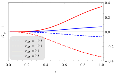
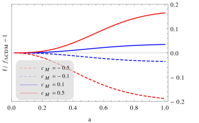
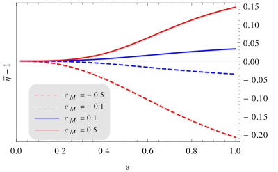
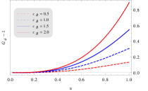
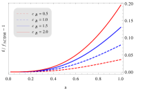
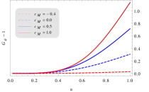
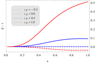
In Fig. (1) we show the evolution of the effective Newton’s constant $G_{\Psi}$ top panel), the growth rate $f$ (central panel) and the slip parameter $\bar{\eta}$ (bottom panel) as a function of the scale factor. Increasing the value of $\left|c_{\textrm{M}}\right|$ is equivalent to increase the deviations w.r.t. the standard values $G_{\Psi}=1$, $f=f_{\Lambda\textrm{CDM}}$ and $\bar{\eta}=1$. Note that the extreme models, $c_{M}=\pm 0.5$, are already disfavoured from current data as they induce effects on observable quantities that are larger than the limit of Eq. (3.1). Thus $c_{M}\lesssim 0.2$ but for forecasted errors from future surveys, should there be no deviations from standard cosmology, then $c_{M}\ll 0.1$.

Figure 1: Evolution of the effective Newton’s constant $G_{\Psi}$ (top panel), the linear growth rate $f$ (central panel) and the slip parameter $\bar{\eta}$ (bottom panel) as a function of the scale factor $a$. In all the panels we take the relative deviations w.r.t. our fiducial model, i.e. $\Lambda\textrm{CDM}$. Starting from the bottom lines, the different models are $c_{\textrm{M}}=-0.5$ (red dashed line), $c_{\textrm{M}}=-0.1$ (blue dashed line), $c_{\textrm{M}}=0.1$ (blue solid line) and $c_{\textrm{M}}=0.5$ (red solid line).

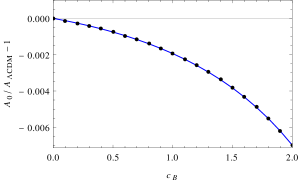
In Fig. (2) we show the second-order interesting quantities. In particular, in the left panel we plot the value of $A_{0}(a=1)$, Eq. (2.17), normalized by its value in a $\Lambda\textrm{CDM}$ universe as a function of the parameter $c_{\textrm{M}}$. One can see that for small values of $c_{\textrm{M}}$ the standard limit is recovered, while one can reach deviations of the order of $1\%$ when $c_{\textrm{M}}=1$. However such large value for $c_{M}$ induces uncomfortably large changes on first-order quantities, see discussion around Fig. (1). We can conclude that $A_{0}$ in Eq. (2.17) is effectively standard. Therefore the only models that have a chance to significantly change the bispectrum are those where $\alpha_{5},\alpha_{4}$ are non-zero.

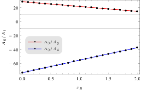
In the right panel we plot the values of $A_{0}/A_{5}$ and $A_{0}/A_{4}$, Eq. (2.17), calculated today as a function of $c_{\textrm{M}}$. In the relevant range for $c_{\textrm{M}}$, $A_{5}$ is 10 to 20 times smaller than $A_{0}$ and $|A_{4}|$ is 20 to 40 times smaller than $A_{0}$. The ratio $A_{0}/A_{i}$ therefore indicates how large the parameters $\{c_{5},c_{4}\}$ have to be in order to modify the bispectrum kernel, Eq. (2.16). The result is that, in the limit $c_{\textrm{M}}\rightarrow 0$ or when it is negative we need $\{c_{5},c_{4}\}\gtrsim\{1,2\}$ in order to have a kernel modified by $10\%$ and $\{c_{5},c_{4}\}>\{0.1,0.2\}$ to have a kernel modified by more than 1%. When $c_{\textrm{M}}\rightarrow 1$, we need even larger values of $\{c_{5},c_{4}\}$ to have the same deviation.

Figure 2: In the left panel we show the relative deviation of $A_{0}$ w.r.t. $A_{\Lambda\textrm{CDM}}$, i.e. $A_{0}$ for a pure $\Lambda\textrm{CDM}$, for different models. In the right panel $A_{0}/A_{5}$ (red line) and $A_{0}/A_{4}$ (blue line). In both panels the quantities are calculated today as a function of $c_{\textrm{M}}$. We vary the parameter $c_{\textrm{M}}$ from $-0.5$ to $1$, since the upper and the lower values already show significant deviations at first-order (e.g. Fig. 1). The left panel shows that the standard term of the kernel, Eq. (2.16), have deviations w.r.t. the GR one $\lesssim 1\%$ for all the cases under consideration. The right panel shows that $c_{5}$ and $c_{4}$ should be $\gtrsim 1$ in order to have an interesting effect on the bispectrum kernel.

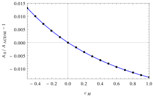
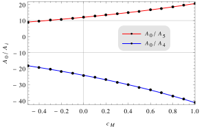
In conclusion, for models with negligible braiding, it is necessary to require $c_{\textrm{M}}\ll 1$ in order to have the evolution of the linear perturbations not in tension with current constraints, Eq. (3.1) [60, 61]. As shown in Fig. 2, at second-order the kernel, Eq. (2.16), is weakly dependent on the value of $c_{\textrm{M}}$ and its modifications are mostly due to the parameters $c_{5},c_{4}$. It is possible to note that the kernel is modified by less than $1\%$ w.r.t. the standard one if we impose $c_{5},c_{4}\lesssim 0.1$. Differences of order $10\%$ can arise for models with $c_{5},c_{4}\gtrsim 1$. Then, an interesting bispectrum kernel modification can happen only if the parameters of the DE/MG model we consider do not satisfy the expected natural hierarchy, Eq. (2.9).

3.2 Large braiding

Here we want to study models that evolve on sub-braiding scales. For these models we expect a more interesting physics, since the braiding causes the DE to cluster on linear scales. On the other hand, the equations are longer and there are no reduction on the linear-order free parameters. We then explore the parameter space $\{c_{\textrm{B}},c_{\textrm{M}},c_{\textrm{T}}\}$ using two grids of 30 points in each direction. As we shall see, the dependence of the interesting first and second-order functions on the parameters is smooth, then the choice of using just 30 points is justified. For generic DE/MG models falling in our description, the expected values for the free parameters are naturally $\mathcal{O}\left(1\right)$. Then, for the first grid we assumed $c_{\textrm{B}}\in\left[-3;3\right]$, $c_{\textrm{M}}\in\left[-1.5;1.5\right]$ and $c_{\textrm{T}}\in\left[-0.75;0.75\right]$. We used the second grid to focus on those models that have parameters closer to their standard value (i.e. zero): $c_{\textrm{B}}\in\left[-1;1\right]$, $c_{\textrm{M}}\in\left[-0.5;0.5\right]$ and $c_{\textrm{T}}\in\left[-0.5;0.5\right]$. With $c_{\textrm{M}}$, and in particular with $c_{\textrm{T}}$, we have been more restrictive than with $c_{\textrm{B}}$, since they regulate the non-minimal coupling of the theory and they have a bigger effect on the evolution of perturbations. Thus, our bounds can be considered representative of the full parameter space. Here, it is important to recall that the kineticity, $\alpha_{\textrm{K}}$, does not appear in the QS equations, Eqs. (2.11-2.12). Then, it is always possible to tune the coefficient $c_{\textrm{K}}$ in order to satisfy the large braiding condition, i.e. $\alpha_{\textrm{B}}^{2}\gg\alpha_{\textrm{K}}$, without modifying our results. For each point we check the stability conditions, we calculate the value for the fractional deviation of the growth rate today w.r.t. $\Lambda\textrm{CDM}$, i.e. $f\left(a=1\right)/f_{\Lambda}\left(a=1\right)-1$, the effective Newton’s constant, i.e. $G_{\Psi}\left(a=1\right)-1$, and the slip parameter, i.e. $\bar{\eta}\left(a=1\right)-1$. We then estimate the values of the functions $A_{0}/A_{\Lambda}$, $A_{0}/A_{5}$ and $A_{0}/A_{4}$.

If we require that the linear order quantity $f$ should not be modified by more than $6\%$ w.r.t. standard gravity, Eq. (3.1), we find that the second-order parameters should be at least $c_{5},c_{4}\gtrsim 2(1)$ in order to have an effect of at least $10\%(3\%)$ on the kernel Eq. (2.16).

If we want to keep $c_{5},c_{4}$ small ($\lesssim 1$) and have large modifications on the kernel $\sim 10\%$ ($3\%$) we have to allow for deviations of $\sim 30\%$ ($10\%$) at linear-order. However, to find signatures of these kind of models, a higher-order correlations (and thus second-order) analysis is not needed, since any signature of DE/MG could be seen easily using observables that rely on linear theory. There are few exceptions to this result in the region of the parameter space where $c_{\textrm{T}}\sim-0.5$. Here we can keep $c_{5},c_{4}$ small ($\lesssim 1$), have deviations on the linear growth rate $\lesssim 6\%$ and have large deviations on the bispectrum kernel ($\sim 10\%$). However, such $c_{\textrm{T}}$ values imply a speed of tensors significantly smaller than the speed of light which can be ruled out by observations of ultra-high energy cosmic rays [64, 65, 66].

In Fig. (3) we show the linear evolution for few representative models. The left panels refer to the effective Newton’s constant, in the central panels we plot the linear growth rate and in the right panels we show the time evolution of the slip parameter. In the top panels we present the behaviour of a minimally coupled theory ($c_{\textrm{M}}=c_{\textrm{T}}=0$). We vary $c_{\textrm{B}}$ in the region where ghost and gradient instabilities are avoided, i.e. $c_{\textrm{B}}>0$. It is possible to note that $c_{\textrm{B}}$ enhances the effective Newton’s constant and the linear growth. This is expected, and it is the signal of a stronger gravity, which should be screened on small scales to satisfy solar system constraints. It is also expected the absence of anisotropic stress (top right panel), since $\bar{\eta}\neq 1$ only in non-minimally coupled theories. In the central panels we fix $c_{\textrm{B}}=1$ and $c_{\textrm{T}}=0$, letting $c_{\textrm{M}}$ free to vary. In this case we can compensate the effect of the braiding by choosing a negative value for $c_{\textrm{M}}$. By fixing $c_{\textrm{M}}\simeq-0.4$ we can recover nearly the standard predictions for $G_{\Psi}$, but the growth rate $f$ appears slightly suppressed. This is because in our description $c_{\textrm{M}}$ affects directly the evolution of the matter density through Eq. (2.6). Finally, in the bottom panels we show the evolution of $G_{\Psi}$, $f$ and $\bar{\eta}$ for different values of $c_{\textrm{T}}$. We set $c_{\textrm{B}}=1$ and $c_{\textrm{M}}=0$. Note that we have chosen extreme values for $c_{\textrm{T}}$, and $c_{\textrm{T}}=-0.5$ could be ruled out by the Cherenkov radiation emission argument [64, 65, 66]. Despite this fact, the parameter $c_{\textrm{T}}$ seems to affect the evolution of linear perturbations less than the others.

Figure 3: Evolution of the effective Newton’s constant $G_{\Psi}$ (left panels), the linear growth rate $f$ (central panels) and the slip parameter $\bar{\eta}$ (right panels) as a function of the scale factor $a$. In every panel we take the relative deviations w.r.t. our fiducial model, i.e. $\Lambda\textrm{CDM}$. In the top panels we fix $c_{\textrm{M}}=c_{\textrm{T}}=0$ and we vary $c_{\textrm{B}}=0.5$ (red dashed lines), $c_{\textrm{B}}=1.0$ (blue dashed lines), $c_{\textrm{B}}=1.5$ (blue solid lines) and $c_{\textrm{B}}=2.0$ (red solid lines). In the central panels we fix $c_{\textrm{T}}=0$, $c_{\textrm{B}}=1$ and we vary $c_{\textrm{M}}=-0.4$ (red dashed lines), $c_{\textrm{M}}=0$ (blue dashed lines), $c_{\textrm{M}}=0.5$ (blue solid lines) and $c_{\textrm{M}}=0.5$ (red solid lines). In the bottom panels we fix $c_{\textrm{M}}=0$, $c_{\textrm{B}}=1$ and we vary $c_{\textrm{T}}=-0.5$ (red dashed lines), $c_{\textrm{T}}=0$ (blue dashed lines), $c_{\textrm{T}}=0.5$ (blue solid lines) and $c_{\textrm{T}}=1$ (red solid line).

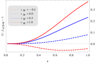
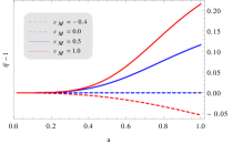
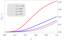
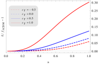
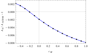
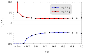
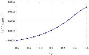
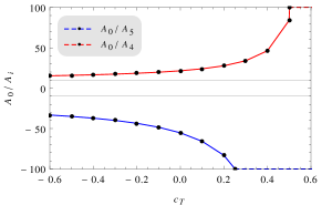
As in the previous section, to understand the bispectrum modifications we focus on the functions $\{A_{0},A_{5},A_{4}\}$. In Fig. (4) we show the value assumed today by $A_{0}$ (left panels) and $A_{5}$ and $A_{4}$ (right panels) as a function of $c_{\textrm{B}}$ (top panels), $c_{\textrm{M}}$ (central panels) and $c_{\textrm{T}}$ (bottom panels). For all the models under consideration $A_{0}$ deviates from its standard value by less than $1\%$. Therefore also in this case this function cannot be responsible for large deviations in the bispectrum and only models with non-zero $\alpha_{5}$ and $\alpha_{4}$ can modify it. Also the functions $A_{5}$ and $A_{4}$ appear rather suppressed compared to $A_{0}$. Indeed, $\left|A_{0}/A_{i}\right|>10$ for every model under consideration. Moreover, for some value of $c_{\textrm{M}}$ (central right panel) and $c_{\textrm{T}}$ (bottom right panel) the curves apparently diverge. For these models $\left|A_{5},A_{4}\right|\ll A_{0}$, which indicates that these terms can not realistically modify the bispectrum kernel. In the cases where $\left|A_{0}/A_{i}\right|$ is minimized we still need to choose $c_{5},c_{4}\gtrsim 1$ in order to achieve deviations in the kernel of at least $10\%$ . One could argue that these deviation can be reached without imposing $c_{5},c_{4}\gtrsim 1$ just by increasing the braiding $c_{\textrm{B}}$. However, comparing these plots with the ones in Fig. (3) we note that the limit $c_{\textrm{B}}\gg 1$ produces large modifications of the first-order evolution. Even if we introduce a negative $c_{\textrm{M}}$ to compensate the linear-order deviations we expect for $A_{5}$ and $A_{4}$ to be further suppressed (see central-right panel of Fig. (4)).

In conclusion, even for general models with large braiding, at second-order in perturbation theory we can not produce large deviations in the bispectrum kernel for models that respect the expected hierarchy, Eq. (2.4) without generating even larger effects at first order.

Figure 4: In the left panels we show $A_{0}/A_{\Lambda\textrm{CDM}}$ evaluated today, while in the right panels we show $A_{0}/A_{5}$ (red line) and $A_{0}/A_{4}$ (blue line) evaluated today. In the top panels we fix $c_{\textrm{M}}=c_{\textrm{T}}=0$ and we vary $c_{\textrm{B}}$. In the central panels we fix $c_{\textrm{T}}=0$, $c_{\textrm{B}}=1$ and we vary $c_{\textrm{M}}$. In the bottom panels we fix $c_{\textrm{M}}=0$, $c_{\textrm{B}}=1$ and we vary $c_{\textrm{T}}$. In the left panels it is possible to note that the standard term of the kernel, Eq. (2.16), have deviations w.r.t. the GR one $\lesssim 1\%$ for every case under consideration. The right panels show that $c_{5}$ and $c_{4}$ should be $\gtrsim 2$ in order to have an interesting effect on the bispectrum kernel ($\sim 10\%$). In the right central and bottom panels it is possible to note divergencies in the curves for $c_{\textrm{M}}=-0.5$ and $c_{\textrm{T}}=0.6$ respectively. Indeed for these models $\left|A_{5},A_{4}\right|\ll A_{0}$, which is a sign that these terms can not realistically modify the bispectrum kernel.

3.3 Bispectrum shapes

In this section we show how the shape of the bispectrum is modified for Horndeski-type DE/MG models. This is useful in order to estimate what are the configurations for which the modifications of the bispectrum kernel, if any, are maximised, i.e., the easiest to detect. In the previous sections we considered the evolution of the function $C\left(t\right)$ and we showed that it is unnatural to have large modifications in $C\left(t\right)$ evaluated today. This is the only modification that appears in the bispectrum kernel, Eq. (2.16), and, its magnitude at any particular time, is just a number. Therefore here in full generality we do not consider particular models, just the value of $C\left(z_{obs}\right)$, where $z_{obs}$ is the redshift at which we want to measure the bispectrum. We perturb $C\left(z_{obs}\right)$ from it standard value ($C_{\Lambda\textrm{CDM}}\simeq 1.62$) by fixed percentages ($1\%$, $2\%$, $5\%$, $10\%$). Recall that the deviations in the bispectrum kernel are maximised today and vanish at early times by construction. However, forthcoming and future surveys do not measure the bispectrum today, but at higher redshifts ($z\sim 0.5-1$). Then, our main result, i.e. the modifications of the bispectrum for natural models are $\lesssim 1\%$ today, can be considered as an upper bound on the modifications of the bispectrum that a generic survey will measure if gravity satisfies our naturalness condition.

Instead of using the bispectrum itself, Eq. (1.8), we consider the reduced bispectrum [67, 68]

$$Q\left(t,\vec{k}_{1},\vec{k}_{2},\vec{k}_{3}\right)\equiv\frac{B\left(t,\vec{k}_{1},\vec{k}_{2},\vec{k}_{3}\right)}{P\left(t,\vec{k}_{1}\right)P\left(t,\vec{k}_{2}\right)+cyc.}=\frac{F_{2}\left(t,\vec{k}_{1},\vec{k}_{2}\right)\,P\left(t,k_{1}\right)\,P\left(t,k_{2}\right)+cyc.}{P\left(t,\vec{k}_{1}\right)P\left(t,\vec{k}_{2}\right)+cyc.}\,,$$ (3.2)

which removes most of the cosmology and scale dependence. Here, the PS can be written as

$$P\left(t,\vec{k}\right)\propto\delta_{+}^{2}\left(t\right)\,T^{2}\left(k\right)\,\left(\frac{k}{H_{0}}\right)^{n_{s}},$$ (3.3)

where $\delta_{+}\left(t\right)$ is the growing solution of Eq. (2.13) and encodes all the time dependence of the PS. $T\left(k\right)$ is the transfer function, which we take as standard using the fitting formula given in [69]. This is consistent with our parametrization, since we only allow for modifications at late-times while we assume that the Universe behaves as standard during the epochs dominated by radiation and matter. Finally $n_{s}$ is the scalar spectral index, and we fix it at $n_{s}=0.96$ [4]. It is important to keep in mind that, since we are looking at models either sub or super-braiding, the growth of perturbations is not scale dependent. As a consequence, one can see using Eqs. (3.2-3.3), the only time dependence in the reduced bispectrum appears in the kernel $F_{2}$, and thus in $C\left(t\right)$.

Figure 5: We show the reduced bispectrum $Q$ (top panels) and its relative deviations w.r.t. the reduced bispectrum of our fiducial model $Q_{\Lambda\textrm{CDM}}$ (bottom panels) for different configurations. In every panel $Q$ is plotted as a function of the angle $\theta_{12}\equiv\arccos\left(\mu\right)=\arccos\left(\frac{\vec{k}_{1}\cdot\vec{k}_{2}}{k_{1}k_{2}}\right)$. In the left panels we fix $k_{1}=k_{2}=0.01\,h\,Mpc^{-1}$, in the right panels $k_{1}=2\times k_{2}=0.02\,h\,Mpc^{-1}$. $\Delta C$ represents the relative modifications of the function $C$, i.e. $\Delta C\equiv\frac{C-C_{\Lambda\textrm{CDM}}}{C_{\Lambda\textrm{CDM}}}$. The models we plot are: $\Delta C=0.01$ (red dashed lines), $\Delta C=0.02$ (blue dashed lines), $\Delta C=0.05$ (red solid lines) and $\Delta C=0.10$ (blue solid lines). Note that in both panels the effects of a modified bispectrum kernel are maximised for $\theta_{12}\simeq 0.6\pi$, where their magnitude reaches $\sim 3\times\Delta C$.

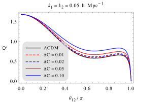
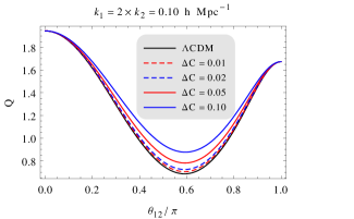
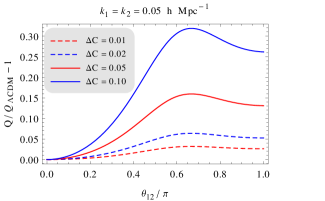
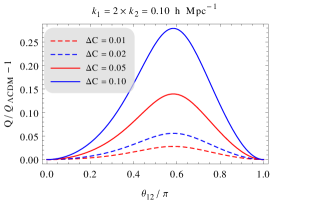
In Fig. (5), we show the shape of the reduced bispectrum $Q$, Eq. (3.2), and its relative deviations w.r.t. the reduced bispectrum of our fiducial model ($Q_{\Lambda\textrm{CDM}}$) as a function of the angle $\theta_{12}\equiv\arccos\left(\mu\right)=\arccos\left(\frac{\vec{k}_{1}\cdot\vec{k}_{2}}{k_{1}k_{2}}\right)$. In the left panels we fix $k_{1}=k_{2}=0.05\,h\,Mpc^{-1}$, while in the right panels we fix $k_{1}=2\times k_{2}=0.10\,h\,Mpc^{-1}$. The different curves show the behaviour of $Q$ for different values of $\Delta C$, which represents the relative modifications of the function $C$ w.r.t. our fiducial model, i.e. $\Delta C\equiv\frac{C-C_{\Lambda\textrm{CDM}}}{C_{\Lambda\textrm{CDM}}}$. It is important to note that in the left panel the limit $\theta_{12}\rightarrow\pi$ involve extremely large scales ($k_{i}\rightarrow 0$). Then, since we are assuming to be well inside or outside the braiding scale, Eq. (2.10), the behaviour of the curves in these limits could probably be corrected for real models.

In every panel the differences in the reduced bispectrum are maximised at $\theta_{12}\simeq 0.6\pi$, where they are three times bigger than the differences in $C$, i.e. $\Delta Q\sim 3\Delta C$. For all the other configurations the deviations from the standard bispectrum are suppressed. This can be connected with the findings of the previous sections, where we considered modifications in $C$ of $\sim 3\%$ as large ones. Indeed, the observable is $Q$ in particular configurations, and not $C$. Then, we have been conservative in considering the maximum deviations as the deviations that could be detected by forthcoming and future surveys. Comparing Fig. (5) with the reduced bispectrum obtained by considering bias or non-linear corrections (e.g. [38]), we see that the Horndeski modifications of the DM bispectrum kernel, Eq. (2.16), are qualitatively different.

4 Conclusions

We have presented a systematic analysis of the DM bispectrum generated at late-times by gravitational instability in the general Horndeski class of models. We assumed a $\Lambda\textrm{CDM}$ evolution for the Hubble function $H\left(t\right)$ and we parametrized the perturbations. In this way we were able to separate the effects of the expansion history of the Universe from the first and second-order effects.

We focused on two class of models, the ones with large braiding ($\alpha_{\textrm{B}}^{2}\gg\alpha_{\textrm{K}}$) and the ones with small braiding ($\alpha_{\textrm{B}}^{2}\ll\alpha_{\textrm{K}}$). In the intermediate regime, where $\alpha_{\textrm{B}}^{2}\sim\alpha_{\textrm{K}}$, we expect the linear evolution of perturbations to be scale-dependent. Then, any deviation from standard gravity can be seen looking, e.g.,  at the PS without the need of a bispectrum analysis.

In the small braiding case we noted that the only parameter that is left free to vary at linear-order is the Planck mass run-rate ($c_{\textrm{M}}$). Then, we showed that, even if we allow for large deviations at linear-order $\sim 10\%$ ($\sim 1\%$) we can not have large modifications at second-order $\sim 3\%$ ($\sim 1\%$) if $c_{5},c_{4}\lesssim c_{\textrm{M}},c_{\textrm{T}}$. Since the parameters $c_{5}$ and $c_{4}$ represent the second-order contribution of non minimal coupling between the metric $g_{\mu\nu}$ and the scalar field $\phi$, they can be seen as corrections of the linear parameters $c_{\textrm{M}}$ and $c_{\textrm{T}}$. This argument leads to Eq. (2.4), which we consider to be the natural behaviour of realistic DE/MG models.

The large braiding case is more complicated. We then explored the parameter space for realistic values of $\{c_{\textrm{B}},c_{\textrm{M}},c_{\textrm{T}}\}$. We found that, assuming that the linear growth $f$ is measured with a $6\%$ precision (or better), there can not be significant deviations in the bispectrum if $c_{5},c_{4}\lesssim c_{\textrm{M}},c_{\textrm{T}}$. The only way of having large modifications in the bispectrum kernel ($\sim 3\%$) with $c_{5},c_{4}\lesssim c_{\textrm{M}},c_{\textrm{T}}$, is to allow for unrealistic deviations on the growth rate $f$ ($\sim 30\%$). These models are expected to be excluded by linear observations, without the need of the analysis of the bispectrum.

Large and observable modifications of the DM bispectrum kernel are still possible in the Horndeski class of models. However, they can not come from the function $A_{0}$ in Eq. (2.17), since it can be modified by $\lesssim 1\%$ for all the models under consideration. Indeed, only models with with large $\alpha_{5}$ and $\alpha_{4}$, i.e. $\alpha_{5},\alpha_{4}\gg\alpha_{\textrm{M}},\alpha_{\textrm{T}}$, have a chance to modify it. Note that in popular MG models such as as Brans-Dicke/f(R), kinetic gravity braiding, cubic galileons these functions are zero. It is therefore not surprising that no significant signatures of these models in the bispectrum were found in these cases. Large $\alpha_{5}$, $\alpha_{4}$ imply a large non-minimal coupling between the curvature and the derivatives of the scalar field. This can be achieved in, e.g., quartic and quintic galileons at the price of having large $\alpha_{\textrm{M}}$ and $\alpha_{\textrm{T}}$.

In conclusion, we have shown that it is not possible to have large modifications in the DM bispectrum kernel for models following our parameterisation of the free Horndeski functions and that satisfy our naturalness condition, Eq. (2.4), without introducing even larger changes in first-order quantities. Even if in these models there is no extra qualitatively new information in the DM bispectrum, we are certainly not advocating not to use it. Our findings imply that the kernel, Eq. (2.16), can be modelled as the standard GR one and applied more generally. Such bispectrum analysis is still useful to: 1) have new information on real word effects, e.g., bias parameters, to remove degeneracies; 2) decrease statistical errors; 3) offer a powerful consistency check.

Eq. (2.4) can be seen as a prescription, under which we can consider the DM bispectrum kernel as standard. Then, the observation of a large bispectrum deviation that can not be explained in terms of bias would imply either that the linear evolution of perturbations is strongly different than the evolution predicted by GR or that the theory of gravity is exotic and/or fine-tuned.

Appendix A Formulas

In this Section we present the equations that are too long to fit in the main text. In particular, the second-order $\alpha_{i}$ functions in Sec. 2 read

$$M_{*}^{2}\alpha_{5}\equiv 2\dot{\phi}HXG_{5X}$$ (A.1)

$$M_{*}^{2}\alpha_{4}\equiv -2X\left(G_{4X}+2XG_{4XX}-G_{5\phi}-XG_{5\phi X}\right)-2\dot{\phi}HX^{2}G_{5XX}\,,$$ (A.2)

where the functions $G_{4,5}$ are the Horndeski functions and their derivatives defined in Eq. (1.1).

The modified Newton’s constants in Eqs. (2.11-2.12) are

$$G_{\Psi}= 1-\frac{\left(\alpha_{\textrm{B}}+2\alpha_{\textrm{M}}\right)^{2}H^{2}-\alpha_{\textrm{T}}\left[2\left(2\dot{H}+\tilde{\rho}_{\textrm{m}}\right)-2\left(H\alpha_{\textrm{B}}\right)^{.}+H^{2}\left(2-\alpha_{\textrm{B}}\right)\left(\alpha_{\textrm{B}}+2\alpha_{\textrm{M}}\right)\right]}{2\left(2\dot{H}+\tilde{\rho}_{\textrm{m}}\right)-2\left(H\alpha_{\textrm{B}}\right)^{.}-H^{2}\left(2-\alpha_{\textrm{B}}\right)\left[\alpha_{\textrm{B}}+2\alpha_{\textrm{M}}-\alpha_{\textrm{T}}\left(2-\alpha_{\textrm{B}}\right)\right]}$$ (A.3)

$$G_{\Phi}= 1-\frac{\alpha_{\textrm{B}}H^{2}\left[\alpha_{\textrm{B}}+2\alpha_{\textrm{M}}-\alpha_{\textrm{T}}\left(2-\alpha_{\textrm{B}}\right)\right]}{2\left(2\dot{H}+\tilde{\rho}_{\textrm{m}}\right)-2\left(H\alpha_{\textrm{B}}\right)^{.}-H^{2}\left(2-\alpha_{\textrm{B}}\right)\left[\alpha_{\textrm{B}}+2\alpha_{\textrm{M}}-\alpha_{\textrm{T}}\left(2-\alpha_{\textrm{B}}\right)\right]}\,.$$ (A.4)

At second-order, the function $C\left(t\right)$ that modifies the bispectrum kernel, Eq. (2.16), reads

$$C\left(t\right)\equiv\int_{0}^{t}\frac{dt^{\prime}\delta_{g}^{2}\left(t^{\prime}\right)}{W\left(t^{\prime}\right)\delta_{g}^{2}\left(t\right)}\left[\delta_{d}\left(t\right)\delta_{g}\left(t^{\prime}\right)-\delta_{g}\left(t\right)\delta_{d}\left(t^{\prime}\right)\right]c\left(t^{\prime}\right)\,,$$ (A.5)

where $\delta_{g}$ and $\delta_{d}$ are the growing and the decaying modes of Eq. (2.13) respectively, while $W\left(t\right)\equiv\delta_{g}\left(t\right)\delta^{\prime}_{d}\left(t\right)-\delta^{\prime}_{g}\delta_{d}\left(t\right)\left(t\right)$ is the Wronskian. Finally $c\left(t\right)$ is defined as

$$c\left(t\right)= \tilde{\rho}_{\textrm{m}}G_{\Psi}+\frac{8}{3}H^{2}f^{2}+\frac{\tilde{\rho}_{\textrm{m}}^{2}}{3H^{2}\alpha_{\textrm{B}}^{2}}\left(3+2\alpha_{\textrm{T}}-3G_{\Psi}\right)\left(1-G_{\Phi}\right)^{2}$$ (A.6)

$$+\frac{2\tilde{\rho}_{\textrm{m}}^{2}\left(1+\alpha_{\textrm{T}}-G_{\Psi}\right)\left(1-G_{\Phi}\right)}{3H^{2}\alpha_{\textrm{B}}^{2}\left[\alpha_{\textrm{B}}\left(1+\alpha_{\textrm{T}}\right)+2\left(\alpha_{\textrm{M}}-\alpha_{\textrm{T}}\right)\right]}\left[\left(\alpha_{\textrm{B}}-2\alpha_{\textrm{M}}\right)\left(1-G_{\Phi}\right)-2\alpha_{\textrm{B}}\alpha_{\textrm{T}}\right]$$

$$-\frac{4\tilde{\rho}_{\textrm{m}}^{2}\left(1+\alpha_{\textrm{T}}-G_{\Psi}\right)\left(1-G_{\Phi}\right)^{2}\dot{\alpha}_{4}}{3H^{3}\alpha_{\textrm{B}}^{2}\left[\alpha_{\textrm{B}}\left(1+\alpha_{\textrm{T}}\right)+2\left(\alpha_{\textrm{M}}-\alpha_{\textrm{T}}\right)\right]}-\frac{2\tilde{\rho}_{\textrm{m}}^{2}\left(1-G_{\Phi}\right)^{2}G_{\Psi}\alpha_{4}}{3H^{2}\alpha_{\textrm{B}}^{2}}$$

$$+\frac{4\tilde{\rho}_{\textrm{m}}^{2}\left(1+\alpha_{\textrm{T}}-G_{\Psi}\right)\left(1-G_{\Phi}\right)\left[\left(1-G_{\Phi}\right)\left(1-\alpha_{\textrm{M}}\right)-\alpha_{\textrm{B}}G_{\Psi}\right]\alpha_{4}}{3H^{2}\alpha_{\textrm{B}}^{2}\left[\alpha_{\textrm{B}}\left(1+\alpha_{\textrm{T}}\right)+2\left(\alpha_{\textrm{M}}-\alpha_{\textrm{T}}\right)\right]}$$

$$+\frac{\tilde{\rho}_{\textrm{m}}^{2}\left(1+\alpha_{\textrm{T}}-G_{\Psi}\right)\left(1-G_{\Phi}\right)\left[2\left(1-G_{\Phi}\right)+\alpha_{\textrm{B}}\left(1-3G_{\Phi}\right)\right]}{3H^{2}\alpha_{\textrm{B}}^{2}\left[\alpha_{\textrm{B}}\left(1+\alpha_{\textrm{T}}\right)+2\left(\alpha_{\textrm{M}}-\alpha_{\textrm{T}}\right)\right]}\left(\frac{\alpha_{5}}{H}\right)^{.}$$

$$-\frac{\tilde{\rho}_{\textrm{m}}^{2}\left(1-G_{\Phi}\right)^{2}}{3\alpha_{\textrm{B}}^{2}H^{2}}\left(\frac{\alpha_{5}}{H}\right)^{.}+\frac{\tilde{\rho}_{\textrm{m}}^{2}\left(1-G_{\Phi}\right)^{2}\left(1+2G_{\Psi}-\alpha_{\textrm{M}}\right)}{3\alpha_{\textrm{B}}^{2}H^{2}}\alpha_{5}$$

$$-\frac{\alpha_{5}\tilde{\rho}_{\textrm{m}}^{2}G_{\Psi}}{3\alpha_{\textrm{B}}H^{2}}\left(1-G_{\Phi}^{2}\right)+\frac{8\dot{H}\tilde{\rho}_{\textrm{m}}^{2}\left(1+\alpha_{\textrm{T}}-G_{\Psi}\right)\left(1-G_{\Phi}\right)^{2}\alpha_{5}}{3H^{4}\alpha_{\textrm{B}}^{2}\left[\alpha_{\textrm{B}}\left(1+\alpha_{\textrm{T}}\right)+2\left(\alpha_{\textrm{M}}-\alpha_{\textrm{T}}\right)\right]}$$

$$-\frac{\tilde{\rho}_{\textrm{m}}^{2}\left(1+\alpha_{\textrm{T}}-G_{\Psi}\right)\left[2\left(1-G_{\Phi}\right)^{2}\left(1-\alpha_{\textrm{M}}\right)-\left(1-2G_{\Phi}\right)\alpha_{\textrm{B}}^{2}G_{\Psi}\right]\alpha_{5}}{3H^{2}\alpha_{\textrm{B}}^{2}\left[\alpha_{\textrm{B}}\left(1+\alpha_{\textrm{T}}\right)+2\left(\alpha_{\textrm{M}}-\alpha_{\textrm{T}}\right)\right]}$$

$$-\frac{\tilde{\rho}_{\textrm{m}}^{2}\left(1+\alpha_{\textrm{T}}-G_{\Psi}\right)\left(1-G_{\Phi}\right)\left[\left(1-3G_{\Phi}\right)\left(1-\alpha_{\textrm{M}}\right)-4G_{\Psi}\right]\alpha_{5}}{3H^{2}\alpha_{\textrm{B}}\left[\alpha_{\textrm{B}}\left(1+\alpha_{\textrm{T}}\right)+2\left(\alpha_{\textrm{M}}-\alpha_{\textrm{T}}\right)\right]}\,.$$

References

- [1] Supernova Cosmology Project Collaboration, S. Perlmutter et al., “Measurements of Omega and Lambda from 42 high redshift supernovae,” Astrophys.J. 517 (1999) 565–586, arXiv:astro-ph/9812133 [astro-ph].
- [2] Supernova Search Team Collaboration, A. G. Riess et al., “Observational evidence from supernovae for an accelerating universe and a cosmological constant,” Astron.J. 116 (1998) 1009–1038, arXiv:astro-ph/9805201 [astro-ph].
- [3] Planck Collaboration, P. Ade et al., “Planck 2013 results. XVI. Cosmological parameters,” Astron.Astrophys. 571 (2014) A16, arXiv:1303.5076 [astro-ph.CO].
- [4] Planck Collaboration, P. Ade et al., “Planck 2015 results. XIII. Cosmological parameters,” arXiv:1502.01589 [astro-ph.CO].
- [5] S. Weinberg, “The Cosmological constant problems,” arXiv:astro-ph/0005265 [astro-ph].
- [6] G. W. Horndeski, “Second-order scalar-tensor field equations in a four-dimensional space,” Int.J.Theor.Phys. 10 (1974) 363–384.
- [7] C. Deffayet, X. Gao, D. Steer, and G. Zahariade, “From k-essence to generalised Galileons,” Phys.Rev. D84 (2011) 064039, arXiv:1103.3260 [hep-th].
- [8] T. Kobayashi, M. Yamaguchi, and J. Yokoyama, “Generalized G-inflation: Inflation with the most general second-order field equations,” Prog.Theor.Phys. 126 (2011) 511–529, arXiv:1105.5723 [hep-th].
- [9] B. Ratra and P. Peebles, “Cosmological Consequences of a Rolling Homogeneous Scalar Field,” Phys.Rev. D37 (1988) 3406.
- [10] C. Wetterich, “Cosmology and the Fate of Dilatation Symmetry,” Nucl.Phys. B302 (1988) 668.
- [11] C. Deffayet, O. Pujolas, I. Sawicki, and A. Vikman, “Imperfect Dark Energy from Kinetic Gravity Braiding,” JCAP 1010 (2010) 026, arXiv:1008.0048 [hep-th].
- [12] T. Kobayashi, M. Yamaguchi, and J. Yokoyama, “G-inflation: Inflation driven by the Galileon field,” Phys.Rev.Lett. 105 (2010) 231302, arXiv:1008.0603 [hep-th].
- [13] O. Pujolas, I. Sawicki, and A. Vikman, “The Imperfect Fluid behind Kinetic Gravity Braiding,” JHEP 1111 (2011) 156, arXiv:1103.5360 [hep-th].
- [14] A. Nicolis, R. Rattazzi, and E. Trincherini, “The Galileon as a local modification of gravity,” Phys.Rev. D79 (2009) 064036, arXiv:0811.2197 [hep-th].
- [15] C. Deffayet, G. Esposito-Farese, and A. Vikman, “Covariant Galileon,” Phys.Rev. D79 (2009) 084003, arXiv:0901.1314 [hep-th].
- [16] S. M. Carroll, V. Duvvuri, M. Trodden, and M. S. Turner, “Is cosmic speed - up due to new gravitational physics?,” Phys.Rev. D70 (2004) 043528, arXiv:astro-ph/0306438 [astro-ph].
- [17] L. Amendola, “Coupled quintessence,” Phys.Rev. D62 (2000) 043511, arXiv:astro-ph/9908023 [astro-ph].
- [18] M. Zumalacárregui, T. S. Koivisto, and D. F. Mota, “DBI Galileons in the Einstein Frame: Local Gravity and Cosmology,” Phys.Rev. D87 (2013) 083010, arXiv:1210.8016 [astro-ph.CO].
- [19] T. S. Koivisto, D. F. Mota, and M. Zumalacarregui, “Screening Modifications of Gravity through Disformally Coupled Fields,” Phys.Rev.Lett. 109 (2012) 241102, arXiv:1205.3167 [astro-ph.CO].
- [20] M. Zumalacárregui and J. García-Bellido, “Transforming gravity: from derivative couplings to matter to second-order scalar-tensor theories beyond the Horndeski Lagrangian,” Phys.Rev. D89 no. 6, (2014) 064046, arXiv:1308.4685 [gr-qc].
- [21] P. Horava, “Quantum Gravity at a Lifshitz Point,” Phys.Rev. D79 (2009) 084008, arXiv:0901.3775 [hep-th].
- [22] D. Blas, O. Pujolas, and S. Sibiryakov, “Consistent Extension of Horava Gravity,” Phys.Rev.Lett. 104 (2010) 181302, arXiv:0909.3525 [hep-th].
- [23] J. Gleyzes, D. Langlois, F. Piazza, and F. Vernizzi, “Healthy theories beyond Horndeski,” arXiv:1404.6495 [hep-th].
- [24] X. Gao, “Unifying framework for scalar-tensor theories of gravity,” Phys.Rev. D90 no. 8, (2014) 081501, arXiv:1406.0822 [gr-qc].
- [25] R. Jimenez, P. Talavera, and L. Verde, “An effective theory of accelerated expansion,” Int.J.Mod.Phys. A27 (2012) 1250174, arXiv:1107.2542 [astro-ph.CO].
- [26] G. Gubitosi, F. Piazza, and F. Vernizzi, “The Effective Field Theory of Dark Energy,” JCAP 1302 (2013) 032, arXiv:1210.0201 [hep-th].
- [27] J. K. Bloomfield, E. E. Flanagan, M. Park, and S. Watson, “Dark energy or modified gravity? An effective field theory approach,” JCAP 1308 (2013) 010, arXiv:1211.7054 [astro-ph.CO].
- [28] J. Gleyzes, D. Langlois, F. Piazza, and F. Vernizzi, “Essential Building Blocks of Dark Energy,” JCAP 1308 (2013) 025, arXiv:1304.4840 [hep-th].
- [29] J. Gleyzes, D. Langlois, F. Piazza, and F. Vernizzi, “Exploring gravitational theories beyond Horndeski,” JCAP 1502 no. 02, (2015) 018, arXiv:1408.1952 [astro-ph.CO].
- [30] J. Gleyzes, D. Langlois, and F. Vernizzi, “A unifying description of dark energy,” Int.J.Mod.Phys. D23 (2014) 3010, arXiv:1411.3712 [hep-th].
- [31] E. Bellini and I. Sawicki, “Maximal freedom at minimum cost: linear large-scale structure in general modifications of gravity,” JCAP 1407 (2014) 050, arXiv:1404.3713 [astro-ph.CO].
- [32] SDSS Collaboration, D. J. Eisenstein et al., “SDSS-III: Massive Spectroscopic Surveys of the Distant Universe, the Milky Way Galaxy, and Extra-Solar Planetary Systems,” Astron.J. 142 (2011) 72, arXiv:1101.1529 [astro-ph.IM].
- [33] M. J. Drinkwater, R. J. Jurek, C. Blake, D. Woods, K. A. Pimbblet, et al., “The WiggleZ Dark Energy Survey: Survey Design and First Data Release,” Mon.Not.Roy.Astron.Soc. 401 (2010) 1429–1452, arXiv:0911.4246 [astro-ph.CO].
- [34] Dark Energy Survey Collaboration, T. Abbott et al., “The dark energy survey,” arXiv:astro-ph/0510346 [astro-ph].
- [35] EUCLID Collaboration, R. Laureijs et al., “Euclid Definition Study Report,” arXiv:1110.3193 [astro-ph.CO].
- [36] H. Gil-Marín, L. Verde, J. Noreña, A. J. Cuesta, L. Samushia, et al., “The power spectrum and bispectrum of SDSS DR11 BOSS galaxies II: cosmological interpretation,” arXiv:1408.0027 [astro-ph.CO].
- [37] H. Gil-Marín, J. Noreña, L. Verde, W. J. Percival, C. Wagner, et al., “The power spectrum and bispectrum of SDSS DR11 BOSS galaxies I: bias and gravity,” arXiv:1407.5668 [astro-ph.CO].
- [38] F. Bernardeau, S. Colombi, E. Gaztanaga, and R. Scoccimarro, “Large scale structure of the universe and cosmological perturbation theory,” Phys.Rept. 367 (2002) 1–248, arXiv:astro-ph/0112551 [astro-ph].
- [39] Y. Takushima, A. Terukina, and K. Yamamoto, “Bispectrum of cosmological density perturbations in the most general second-order scalar-tensor theory,” Phys.Rev. D89 no. 10, (2014) 104007, arXiv:1311.0281 [astro-ph.CO].
- [40] N. Bartolo, E. Bellini, D. Bertacca, and S. Matarrese, “Matter bispectrum in cubic Galileon cosmologies,” JCAP 1303 (2013) 034, arXiv:1301.4831 [astro-ph.CO].
- [41] T. Tatekawa and S. Tsujikawa, “Second-order matter density perturbations and skewness in scalar-tensor modified gravity models,” JCAP 0809 (2008) 009, arXiv:0807.2017 [astro-ph].
- [42] H. Gil-Marín, F. Schmidt, W. Hu, R. Jimenez, and L. Verde, “The Bispectrum of f(R) Cosmologies,” JCAP 1111 (2011) 019, arXiv:1109.2115 [astro-ph.CO].
- [43] F. Bernardeau and P. Brax, “Cosmological Large-scale Structures beyond Linear Theory in Modified Gravity,” JCAP 1106 (2011) 019, arXiv:1102.1907 [astro-ph.CO].
- [44] A. Borisov and B. Jain, “Three-Point Correlations in f(R) Models of Gravity,” Phys.Rev. D79 (2009) 103506, arXiv:0812.0013 [astro-ph].
- [45] C.-P. Ma and E. Bertschinger, “Cosmological perturbation theory in the synchronous and conformal Newtonian gauges,” Astrophys.J. 455 (1995) 7–25, arXiv:astro-ph/9506072 [astro-ph].
- [46] J. M. Bardeen, “Gauge Invariant Cosmological Perturbations,” Phys.Rev. D22 (1980) 1882–1905.
- [47] I. D. Saltas, I. Sawicki, L. Amendola, and M. Kunz, “Anisotropic Stress as a Signature of Nonstandard Propagation of Gravitational Waves,” Phys.Rev.Lett. 113 no. 19, (2014) 191101, arXiv:1406.7139 [astro-ph.CO].
- [48] I. Sawicki and E. Bellini, “Limits of Quasi-Static Approximation in Modified-Gravity Cosmologies,” arXiv:1503.06831 [astro-ph.CO].
- [49] A. De Felice, T. Kobayashi, and S. Tsujikawa, “Effective gravitational couplings for cosmological perturbations in the most general scalar-tensor theories with second-order field equations,” Phys.Lett. B706 (2011) 123–133, arXiv:1108.4242 [gr-qc].
- [50] L. Amendola, M. Kunz, M. Motta, I. D. Saltas, and I. Sawicki, “Observables and unobservables in dark energy cosmologies,” Phys.Rev. D87 no. 2, (2013) 023501, arXiv:1210.0439 [astro-ph.CO].
- [51] M. Motta, I. Sawicki, I. D. Saltas, L. Amendola, and M. Kunz, “Probing Dark Energy through Scale Dependence,” Phys.Rev. D88 no. 12, (2013) 124035, arXiv:1305.0008 [astro-ph.CO].
- [52] N. Bartolo, S. Matarrese, and A. Riotto, “Signatures of primordial non-Gaussianity in the large-scale structure of the Universe,” JCAP 0510 (2005) 010, arXiv:astro-ph/0501614 [astro-ph].
- [53] N. Bartolo, S. Matarrese, and A. Riotto, “CMB Anisotropies at Second-Order. 2. Analytical Approach,” JCAP 0701 (2007) 019, arXiv:astro-ph/0610110 [astro-ph].
- [54] R. Scoccimarro and H. Couchman, “A fitting formula for the nonlinear evolution of the bispectrum,” Mon.Not.Roy.Astron.Soc. 325 (2001) 1312, arXiv:astro-ph/0009427 [astro-ph].
- [55] P. Catelan, F. Lucchin, S. Matarrese, and L. Moscardini, “Eulerian perturbation theory in nonflat universes: Second order approximation,” Mon.Not.Roy.Astron.Soc. 276 (1995) 39, arXiv:astro-ph/9411066 [astro-ph].
- [56] R. Scoccimarro, “The bispectrum: from theory to observations,” Astrophys.J. 544 (2000) 597, arXiv:astro-ph/0004086 [astro-ph].
- [57] F. R. Bouchet, R. Juszkiewicz, S. Colombi, and R. Pellat, “Weakly nonlinear gravitational instability for arbitrary Omega,” Astrophys.J. 394 (1992) L5.
- [58] F. Bernardeau, “Skewness and Kurtosis in large scale cosmic fields,” Astrophys.J. 433 (1994) 1, arXiv:astro-ph/9312026 [astro-ph].
- [59] L. Amendola, S. Fogli, A. Guarnizo, M. Kunz, and A. Vollmer, “Model-independent constraints on the cosmological anisotropic stress,” Phys.Rev. D89 no. 6, (2014) 063538, arXiv:1311.4765 [astro-ph.CO].
- [60] BOSS Collaboration, F. Beutler et al., “The clustering of galaxies in the SDSS-III Baryon Oscillation Spectroscopic Survey: Testing gravity with redshift-space distortions using the power spectrum multipoles,” Mon.Not.Roy.Astron.Soc. 443 (2014) 1065, arXiv:1312.4611 [astro-ph.CO].
- [61] L. Samushia, B. A. Reid, M. White, W. J. Percival, A. J. Cuesta, et al., “The Clustering of Galaxies in the SDSS-III Baryon Oscillation Spectroscopic Survey (BOSS): measuring growth rate and geometry with anisotropic clustering,” Mon.Not.Roy.Astron.Soc. 439 (2014) 3504–3519, arXiv:1312.4899 [astro-ph.CO].
- [62] L. Amendola and C. Quercellini, “Tracking and coupled dark energy as seen by WMAP,” Phys.Rev. D68 (2003) 023514, arXiv:astro-ph/0303228 [astro-ph].
- [63] S. F. Daniel, R. R. Caldwell, A. Cooray, P. Serra, A. Melchiorri, et al., “A Multi-Parameter Investigation of Gravitational Slip,” Phys.Rev. D80 (2009) 023532, arXiv:0901.0919 [astro-ph.CO].
- [64] G. D. Moore and A. E. Nelson, “Lower bound on the propagation speed of gravity from gravitational Cherenkov radiation,” JHEP 0109 (2001) 023, arXiv:hep-ph/0106220 [hep-ph].
- [65] J. W. Elliott, G. D. Moore, and H. Stoica, “Constraining the new Aether: Gravitational Cerenkov radiation,” JHEP 0508 (2005) 066, arXiv:hep-ph/0505211 [hep-ph].
- [66] R. Kimura and K. Yamamoto, “Constraints on general second-order scalar-tensor models from gravitational Cherenkov radiation,” JCAP 1207 (2012) 050, arXiv:1112.4284 [astro-ph.CO].
- [67] E. Groth and P. Peebles, “Statistical analysis of catalogs of extragalactic objects. 7. Two and three point correlation functions for the high - resolution Shane-Wirtanen catalog of galaxies,” Astrophys.J. 217 (1977) 385.
- [68] J. N. Fry and M. Seldner, “Transform analysis of the high-resolution Shane-Wirtanen Catalog - The power spectrum and the bispectrum,” 259 (Aug., 1982) 474–481.
- [69] J. M. Bardeen, J. Bond, N. Kaiser, and A. Szalay, “The Statistics of Peaks of Gaussian Random Fields,” Astrophys.J. 304 (1986) 15–61.
- [70] D. Bettoni and M. Zumalacárregui, “Shaken, not stirred: kinetic mixing in scalar-tensor theories of gravity,” arXiv:1502.02666 [gr-qc].