Standing Electromagnetic Solitons in Degenerate Relativistic Plasmas

Abstract

The existence of standing high frequency electromagnetic (EM) solitons in a fully degenerate overdense electron plasma is studied applying relativistic hydrodynamics and Maxwell equations. The stable soliton solutions are found in both relativistic and nonrelativistic degenerate plasmas.

LABEL:FirstPage1 LABEL:LastPage#11

A significant amount of recent publications describe electromagnetic (EM) waves in relativistic plasmas and majority of them discuss possible roles of these waves in different astrophysical phenomena. Highly relativistic plasmas are observed in the cores of white dwarfs White , in magnetosphere of pulsars Sturok , in the MeV epoch of the early Universe Tajima and additionally, they probably show up in the bipolar jets in Active Galactic Nuclei (AGN) Begelman . Plasma can be relativistic in two following cases: either bulk velocities of fluid cells should be close to the speed of light, or the kinetic energy of particles should be greater then their rest energy. In compact objects, such as white dwarfs and magnetars, the number densities of electrons is believed to be roughly between $10^{26}$ $cm^{-3}$and $10^{34}$ $cm^{-3}$ Shapiro , Shukla-Rev . High density plasma can be produced in the laboratory as well, indeed contemporary petawatt laser systems have the focal intensities $I=2\times 10^{22}$ $W/cm^{2}$ Yanovski . Moreover, pulses with higher than $I=10^{26}W/cm^{2}$ intensities are expected to be achieved soon Dunne . Superdense plasmas might be formed with densities in the range of $10^{23}cm^{-3}$ and $10^{28}cm^{-3}$ Shukla-Eliasson , during the interaction of such EM pulses with solid or gaseous targets. Such plasma will be opaque for conventional laser systems operate at wavelengths $\lambda\sim 1\mu m$. The Linac Coherent Light Source (LCLS) is an $X$-ray free-electron laser produce femtosecond powerful pulses of coherent soft and hard $X$-rays with wavelengths from $2.2nm$ to $0.06nm$ X1 . Exploiting the possibility to focus $X$-ray laser beams on a spot with down to laser wavelength, the focal intensities $I\simeq 7\times 10^{25}$ $W/cm^{2}$ are expected to be reached X2 . Successful operation of $X$-ray free-electron lasers in different centers world wide Keitel opens up new perspectives to study the EM pulse penetration and its subsequent dynamics in super dense plasma in laboratory conditions.

Highly compressed plasma with an average interparticle distance smaller than their thermal de Broglie wavelength, can be considered as a degenerate Fermi gas. When plasma density increases, the more ideal it becomes and the interactions of its particles can be neglected Landau .

EM solitons in classical relativistic plasma is being studied intensively Chveni , but existence and stability of solitary solutions in degenerate quantum relativistic plasma are investigated mostly for low frequencies (see Khan and references therein). The publication goal is to consider existence of a standing, high frequency EM soliton in the relativistic degenerate electron plasma. Importance of the standing soliton solutions for overall dynamics of EM pulses is established theoretically Bul1 - Saxena as well as experimentally for classical relativistic plasma Bor . These publications state, that during interaction of a circularly polarized strong laser pulse and a plasma, part of the laser energy is trapped in non-propagating soliton-like pulses. Similar dynamics is expected in the case of strong EM pulse interaction with degenerate electron plasma.

Plasma can be considered cold, if the thermal energy of its electrons is negligible compared to their Fermi energy. In this case temperature can be assumed to be zero, even though it is of the order of $10^{9}K$ Russo . For the Fermi energy of electrons we have $\epsilon_{F}=m_{e}c^{2}\left[\left(1+R^{2}\right)^{1/2}-1\right]$, where $R=p_{F}/m_{e}c$  and $p_{F}$ is the Fermi momentum. The latter is related to the proper density of electrons $n$ by the following equation $p_{F}=m_{e}c\left(n/n_{c}\right)^{1/3}$, where $n_{c}=5.9\times 10^{29}cm^{-3}$ is the normalizing critical number-density Akbari . Therefore, when $n\geq n_{c}$ , electrons move with relativistic momentum inside plasma unit cells and the plasma can be told as relativistic.

Our investigation is based on the Maxwell equations and fluid model of relativistic electron plasma. The ions are considered to form a stationary neutralizing background. We begin with the manifestly covariant form of the fluid equations for electrons

$$\frac{\partial T^{\alpha\beta}}{\partial x^{\beta}}=-eF^{\alpha\beta}nU_{\beta}$$ (1)

here $\partial_{\alpha}=\partial/\partial x^{\alpha}=\left(c^{-1}\partial/\partial t,\mathbf{\nabla}\right)$; the Greek indexes take values from $0$ to $3$; $T^{\alpha\beta}$ is the energy-momentum tensor describing the plasma electrons with charge $-e$, mass $m_{e}$ and the proper density $n$; the metric tensor is $g^{\alpha\beta}=diag\left(1,-1,-1,-1\right)$; $U^{\alpha}=\left(\gamma,\gamma\mathbf{V/}c\right)$ denotes the local four velocity, here $\gamma=\left(1-V^{2}/c^{2}\right)^{-1/2}$; $\left(U^{\alpha}U_{\alpha}=1\right)$. This equation implies the conservation of energy and momentum. The change of momentum through the collisions is neglected.

We assume, that the total number of electrons is conserved, thus the following continuity equation is held

$$\frac{\partial nU^{\alpha}}{\partial x^{\alpha}}=0$$ (2)

The EM field can be expressed through a tensor $F^{\alpha\beta}=[\mathbf{E},\mathbf{B}]$. The Maxwell equations in these notations are $\partial_{\beta}F^{\alpha\beta}=-(4\pi/c)J^{\alpha}$ and   $\epsilon^{\alpha\beta\gamma\delta}\partial_{\beta}F_{\gamma\delta}=0$. Here $J^{\alpha}=(c\rho,\mathbf{J})$, where $\mathbf{J}$ is the current density and $\rho$ is the total charge density of the plasma.

We use the energy momentum tensor of ideal isotropic fluid $T^{\alpha\beta}=wU^{\alpha}U^{\beta}-g^{\alpha\beta}P$, where $w=E+P$ is the enthalpy per unit volume, $P$ is the pressure and $E$ is density of the rest frame internal energy. If $nT/P<<1$, plasma can be treated as completely degenerate Fermi gas and the following equations are satisfied Chandra

$$P=\frac{m_{e}^{4}c^{5}}{3\pi^{2}\hbar^{3}}f\left(R\right)$$ (3)

$$E=\frac{m_{e}^{4}c^{5}}{3\pi^{2}\hbar^{3}}\left[R^{3}\left(1+R^{2}\right)^{1/2}-f\left(R\right)\right]$$ (4)

where

$$8f\left(R\right)=3\sinh^{-1}R+R\left(1+R^{2}\right)^{1/2}\left(2R^{2}-3\right)$$ (5)

The equation of state for the degenerate gas is $P\propto n^{\Gamma}$, with $\Gamma=5/3$ for nonrelativistic case $\left(R<<1\right)$ and $\Gamma=4/3$ for ultrarelativistic case $\left(R>>1\right)$.

The model of plasma described above implies that the electron distribution function remains locally Juttner-Fermian. In case of zero temperature this results in thermodynamical quantities, depending only on density $E(n),P(n)$ and $w(n)$. Of course, these quantities are functions of $x^{\alpha}$ through the relation $n=N/\gamma$, here $N$ is the electron density in the laboratory reference frame. The considered system is isentropic (furthermore, as temperature approaches zero, entropy tends to zero too). Hence, the following thermodynamic equality is held $d\left(w/n\right)=dP/n$ and taking into account this thermodynamic equality and making some standard manipulations (e.g. Ohashi ), Eq. (1) can be represented in the form of the following system

$$\frac{\partial}{\partial t}\left(G\mathbf{p}\right)+m_{e}c^{2}\mathbf{\nabla}\left(G\gamma\right)=-e\mathbf{E+}\left[\mathbf{V\times\Omega}\right]$$ (6)

$$\frac{\partial}{\partial t}\mathbf{\Omega}=\mathbf{\nabla\times}\left[\mathbf{V\times\Omega}\right]$$ (7)

here, for the generalized vorticity we have $\mathbf{\Omega=-}\left(e/c\right)\mathbf{B+\nabla\times}\left(G\mathbf{p}\right)$ , where $\mathbf{p}=\gamma m_{e}\mathbf{V}$ denotes the hydrodynamic momentum; $G=G(n)$ can be called the density dependent ”effective mass” factor of electrons $G=w/m_{e}nc^{2}=\left(1+R^{2}\right)^{1/2}$. Now dynamics of the degenerate plasma can be completely described by Eqs. (6)-(7) together with Continuity and Maxwell equations. In other words, the set of equations is complete. The analogous set of equations is derived in Ref.Ohashi for classical relativistic plasma obeying Maxwell-Juttner statistics, where $G$ is a function of temperature $G=G(T)$. In contrast, for degenerate plasma $w/m_{e}nc^{2}=\left(1+R^{2}\right)^{1/2}$ and as a result the effective mass factor of electrons depends just on their proper density. The corresponding relation $G=\left[1+\left(n/n_{c}\right)^{2/3}\right]^{1/2}$ holds for any ratio $n/n_{c}$, thus for any strength of relativity BerScr -Beltrami .

We make use of the expressions for fields $\mathbf{B}=\mathbf{\nabla\times A}$ and $\mathbf{E=-(}1/c\mathbf{)\partial A/\partial}t-\mathbf{\nabla}\varphi$ where $\mathbf{A}$ and $\varphi$ are vector and scalar potentials respectively. Applying the Coulomb gauge condition $\mathbf{\nabla\cdot A}=0$, the Maxwell equations take the following form:

$$\frac{\partial^{2}\mathbf{A}}{\partial t^{2}}-c^{2}\Delta\mathbf{A+}c\frac{\partial}{\partial t}\left(\mathbf{\nabla}\varphi\right)-4\pi c\mathbf{J}=0$$ (8)

and

$$\Delta\varphi=-4\pi\rho$$ (9)

where $\mathbf{J}=-e\gamma n\mathbf{V,}$ is the current density and $\rho=e(n_{0}-\gamma n)$ is the charge density, with $n_{0}$ denoting electron (ion) equilibrium density. We use equations (6) and (7) to describe wave dynamics in unmagnetized plasma. Eq. (7) makes clear that if generalized vorticity $\mathbf{\Omega}$ was zero everywhere once, it will stay zero always. Therefore Eq. (6) will reduce to

$$\frac{\partial}{\partial t}\left(G\mathbf{p-}\frac{e}{c}\mathbf{A}\right)+\mathbf{\nabla}\left(m_{e}c^{2}G\gamma-e\varphi\right)=0$$ (10)

Our goal is to find one dimensional localized solutions for equations (8)-(10). Let us assume, that every variable depends on nothing but coordinate $z$ and time $t$. As transverse component of gradient is zero, Eq. (10) easily gives $\mathbf{p}_{\perp}=e\mathbf{A}_{\perp}/(cG)$. Integration constant is zero, because $\mathbf{p}$ should be zero at infinity, where fields vanish. Coulomb gauge condition requires $A_{z}=0$, thus the longitudinal motion of the plasma is driven just by the ”ponderomotive” pressure $\left(\sim\mathbf{p}_{\perp}^{2}\right)$ acting via the relativistic $\gamma$ factor in Eq. (10) ($\gamma=\left[1+\left(\mathbf{p}_{\perp}^{2}+p_{z}^{2}\right)/m_{e}^{2}c^{2}\right]^{1/2}$). The EM pressure forces electrons to move in $z$ direction, the plasma density changes and charge separation occurs. Longitudinal motion of the plasma is described by the following set of equations:

$$\frac{\partial}{\partial t}Gp_{z}+\frac{\partial}{\partial z}\left(m_{e}c^{2}G\gamma-e\varphi\right)=0$$ (11)

while the continuity (2) and Poisson’s equations (9) become

$$\frac{\partial}{\partial t}\gamma n+\frac{\partial}{\partial z}\left(n\gamma V_{z}\right)=0$$ (12)

$$\frac{\partial^{2}\varphi}{\partial z^{2}}=4\pi e(n\gamma-n_{0})$$ (13)

The transverse component of the current density is $\mathbf{J}_{{}_{\perp}}\mathbf{=}\left(ne^{2}/cG\right)\mathbf{A}_{\perp}$ and substituting it into Eq. (8), we get

$$\frac{\partial^{2}\mathbf{A}_{\perp}}{\partial t^{2}}-c^{2}\frac{\partial^{2}\mathbf{A}_{\perp}}{\partial z^{2}}\mathbf{+}\Omega_{e}^{2}\left(\frac{n}{n_{0}}\frac{G_{0}}{G}\right)\mathbf{A}_{\perp}=0$$ (14)

where $n_{0}$ is electron (ion) equilibrium density and $\Omega_{e}=\left(4\pi e^{2}n_{0}/m_{e}^{\ast}\right)^{1/2}$ is the Langmiur frequency of the electron plasma. In this expression $m_{e}^{\ast}$ denotes effective mass of electron $m_{e}^{\ast}=m_{e}G_{0}$, where $G_{0}=\left[1+R_{0}^{2}\right]^{1/2}$ and $R_{0}=\left(n_{0}/n_{c}\right)^{1/3}$.

We are searching for solitary stationary solutions of Eqs. (11)-(14). Assuming electromagnetic wave is circularly polarized, the vector potential can be rewritten as follows $\mathbf{A}_{\perp}=\left[A(z)\cos(\omega t),A(z)\sin(\omega t)\right]$. Here the amplitude $A(z)$ is a real valued function depending only on coordinate $z$ and nothing else. $\omega$ denotes the frequency. It is now convenient to introduce the following dimensionless quantities: $\Psi=e\varphi/\left(m_{e}c^{2}G_{0}\right)$, $a=eA/\left(c^{2}m_{e}G_{0}\right)$, $n=n/n_{0}$, $t=\Omega_{e}t$, $z=\left(\Omega_{e}/c\right)z$. In our case $p_{z}=0$ and integrating Eq. (11) we get the relation

$$\Gamma\gamma=\Psi+1$$ (15)

where

$$\Gamma=\frac{G}{G_{0}}=\sqrt{\frac{1+R_{0}^{2}n^{2/3}}{1+R_{0}^{2}}}$$ (16)

and $\gamma=\left(1+a^{2}/\Gamma^{2}\right)^{1/2}$. Using Eqs. (15)-(16) we obtain the following relationships:

$$n=\frac{1}{R_{0}^{3}}\left[(1+R_{0}^{2})\left[\left(1+\Psi\right)^{2}-a^{2}\right]-1\right]^{3/2}$$ (17)

$$\gamma=\frac{\left(1+\Psi\right)}{\sqrt{\left(1+\Psi\right)^{2}-a^{2}}}$$ (18)

while for the electron density in laboratory frame $\mathcal{N}\left(=n\gamma\right)$ we have

$$\mathcal{N}=\frac{\left(1+\Psi\right)}{\epsilon^{3/2}\left[\left(1+\Psi\right)^{2}-a^{2}\right]^{1/2}}\left[\left(1+\Psi\right)^{2}-(1+a^{2}-\epsilon)\right]^{3/2}$$ (19)

where $\epsilon=R_{0}^{2}/\left(1+R_{0}^{2}\right)$.

The Eqs. (13) and (14) now can be reduced to the following set of ordinary differential equations:

$$\frac{d^{2}a}{dz^{2}}-(1-\omega^{2})a+\left(1-\frac{\mathcal{N}\left(a,\Psi,\epsilon\right)}{1+\Psi}\right)a=0$$ (20)

$$\frac{d^{2}\Psi}{dz^{2}}+1-\mathcal{N}\left(a,\Psi,\epsilon\right)=0$$ (21)

The coupled system of nonlinear equations (19)-(21), where $\mathcal{N}\left(a,\Psi,\epsilon\right)$ is defined by Eq. (19) describes the structure of circularly polarized transverse and longitudinal localized fields in degenerate plasma for arbitrary values of $R_{0}$ $\left(0\leq\epsilon\leq 1\right)$. The general solution of Eqs. (19)-(21) cannot be expressed in terms of elementary functions, it requires numerical methods. However, these equations can be integrated analytically for certain limiting cases. Taking into account that for $\left|z\right|\rightarrow\infty$ the fields vanish $a\rightarrow 0,\Psi\rightarrow 0$ and $\mathcal{N}\rightarrow 1$ we conclude that the standing solitary solutions may exist in an overdense plasma when the frequency of the soliton is less than the electron plasma frequency, $\omega<1$ ($\omega<\Omega_{e}$ - in dimensional units). For any fixed plasma density (i.e. fixed $\epsilon$) the frequency $\omega$ is the only parameter in Eqs. (19)-(21) that defines the characteristics of the solitary solutions. For slightly overdense plasma $\omega\leq 1$ the fields are small $a\ll 1$, $\Psi\ll 1$ while the characteristic width of the structure $L\sim(1-\omega^{2})^{-1/2}>>1$. Applying the quasi-neutrality condition of the plasma ($\mathcal{N\approx}1$) from Eqs. (19) and (21) we get $\Psi\simeq\left(a^{2}/2\right)\left(1-\epsilon/3\right)$ and now Eq. (20) reduces to the simple equation

$$\frac{d^{2}a}{dz^{2}}-(1-\omega^{2})a+\frac{1}{2}\left(1-\epsilon/3\right)a^{3}=0$$ (22)

with the well know soliton solution

$$a=2\sqrt{\frac{1-\omega^{2}}{1-\epsilon/3}}Sech\left[z\sqrt{1-\omega^{2}}\right]$$ (23)

Analytical solutions of Eqs. (19)-(21) can be obtained even for an arbitrary amplitude fields provided that plasma density is small $n_{0}/n_{c}<<1$ ($R_{0}<<1$), implying that the degenerate electron gas is not relativistic. At this end we would like to emphasize that our consideration is valid if the average kinetic energy of electrons ($\sim\epsilon_{F}$) is larger than their interaction energy ($\sim e^{2}n_{0}^{1/3}$). This condition is fulfilled for a sufficiently dense plasma when $n_{0}>>\left(2m_{e}e^{2}/\left(3\pi^{2}\right)^{2/3}\hbar^{2}\right)^{3}=6.3\times 10^{22}cm^{-3}$. For the densities $n_{0}$ in the range from $10^{24}cm^{-3}$ to $10^{28}cm^{-3}$ the corresponding parameter $\epsilon$ is in the range from $1.4\times 10^{-4}$ to $6.2\times 10^{-2}$. Since $\epsilon$ is rather small for the nonrelativistic densities, we can safely assume that $\epsilon\rightarrow 0$ in Eqs. (19)-(20) and then obtain the following relations:

$$\Psi=1-\sqrt{1+a^{2}}$$ (24)

$$\mathcal{N}=1+\frac{d^{2}}{dz^{2}}\sqrt{1+a^{2}}$$ (25)

the wave equation (21) now reduces to

$$\frac{d^{2}a}{dz^{2}}+\omega^{2}a-\frac{a}{\sqrt{1+a^{2}}}\left(1+\frac{d^{2}}{dz^{2}}\sqrt{1+a^{2}}\right)=0$$ (26)

Similar to (24)- (26) system equations have been derived solved in Refs. Kurki , Bulanov where existence and stability of standing EM pulses in cold but classical electron plasma were studied. The soliton solution of Eq. (26) is found to be

$$a=\frac{2\sqrt{1-\omega^{2}}\cosh\left(z\sqrt{1-\omega^{2}}\right)}{\cosh^{2}\left(z\sqrt{1-\omega^{2}}\right)+\omega^{2}-1}$$ (27)

The amplitude of this single hump soliton $a_{m}(=a(0))$ depends on the soliton frequency by the relation $a_{m}=2\sqrt{1-\omega^{2}}/\omega^{4}$. The electrons are depleted from the region of pulse localization. The minimal density at the center of soliton is $\mathcal{N}(z=0)=1-4\left(1-\omega^{2}\right)^{2}/\omega^{4}$Bulanov . Note that for $\omega\rightarrow 1$ the amplitude of soliton decreases and the solution (27) coincides with Eq. (23) where $\epsilon<<1$. With a decrease of $\omega$ the soliton amplitude increases while the corresponding density well deepens. For $\omega=\omega_{c}=\sqrt{2/3}=\allowbreak 0.816$ the electron cavitation takes place $\mathcal{N}(z=0)=0$ while the amplitude of the soliton attains its maximal value $a_{m}=\sqrt{3}$. For $a_{m}>\sqrt{3}$ the solution contains a region where the electron density is negative which implies that wave breaking takes place. Thus, in the nonrelativistic degenerate electron plasma the standing solitons exist provided $\omega_{c}\leq\omega\leq 1$. Similar conclusion has been made in Ref.Eliason by numerical analysis of the coupled set of nonlinear Schrodinger-Poisson equations, where the Bohm potential was introduced in the system. In the fluid approach the Bohm potential is related to the ”quantum force” due to electron tunneling. Our estimations show that this force is small and even for $\omega=\omega_{c}$ it does not change the solution (27) qualitatively.

Now we consider the case of ultrarelativistic degenerate plasma $R_{0}>>1$ ($\epsilon\rightarrow 1$). The system (19)-(21) reduces to the following set of equations

$$\frac{d^{2}a}{dz^{2}}+\omega^{2}a+a\left(a^{2}-\left(1+\Psi\right)^{2}\right)=0$$ (28)

and

Figure 1: The profiles of EM field potentials $a$, $\Psi$ and the electron density $\mathcal{N}$ in case the ultrarelativistic plasma $\epsilon=1$ for the different soliton frequencies (a) $\omega=0.8$ and (b) $\omega=0.7683$.

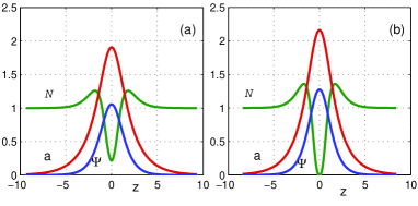
Figure 2: The profiles of EM field potentials and the electron density in case the relativistic plasma with $\epsilon=0.5$ for the different soliton frequencies (a) $\omega=0.8$ and (b) $\omega=0.7694$.

$$\frac{d^{2}\Psi}{dz^{2}}+1+\left(1+\Psi\right)\left(a^{2}-\left(1+\Psi\right)^{2}\right)=0$$ (29)

This system of equations has a first integral (a Hamiltonian)

$$\left[\frac{d\Psi}{dz}\right]^{2}-\left[\frac{da}{dz}\right]^{2}-\omega^{2}a^{2}+2\Psi-\frac{1}{2}\left[a^{2}-\left(1+\Psi\right)^{2}\right]^{2}+\frac{1}{2}=0$$ (30)

where the zero boundary conditions for the fields $\Psi$, $a$ and their derivatives at $\left|z\right|\rightarrow\infty$ have been used.

Fig.1 shows the numerical solution of the system (19)-(21) for different values of the soliton frequency $\omega$. One can see that the structure of the solitary solutions in ultrarelativistic plasma is similar to one, obtained in the nonrelativistic case. The solution has a continuous spectrum with $\omega_{c}\leq\omega\leq 1$ where $\omega_{c}=0.7683$, and it is composed of a single maximum of field potentials ($a,\Psi$) and depleted electron density ($\mathcal{N}$) region at the center of structure. For $\omega\rightarrow 1$ the numerical solution coincides with Eq. (23) (using $\epsilon=1$). For $\omega\simeq\omega_{c}$, amplitude of the soliton becomes relativistically strong $a_{m}\simeq 2.267$, while at the center of the soliton $\mathcal{N}\simeq 0$, i.e. the electron cavitation takes place.

Numerical analysis demonstrates that equations (20)-(21) have soliton-like solutions for any finite value of $R_{0}$. As an example in Fig.2 we plot the numerical solutions of the system for $R_{0}=1$ ($\epsilon=0.5$). The soliton exists for $\omega_{c}\leq\omega\leq 1$, where $\omega_{c}=0.7694$ and at this frequency $a_{m}\simeq 2.162$.

To verify the stability of obtained solutions, we performed 1D simulations applying the numerical code developed in Ref.Berezhiani . The simulations demonstrate exceptional stability of the solution for entire rage of soliton existence described above.

To summarize, in this paper we considered circularly polarized high frequency EM solitons in degenerate electron plasma. We used Maxwell and relativistic fluid equations to demonstrate possibility of stable existence of solitons in overdense plasma ($\omega\leq\Omega_{e}$). Soliton exists for entire range of physically allowed electron densities, presumably for $n_{0}=10^{24}cm^{-3}$ and higher, i.e. in both relativistic and nonrelativistic degenerate plasmas. Intensity of the solitons can be small for $\omega\rightarrow\Omega_{e}$ and becomes relativistically strong ($a_{m}>1$) for $\omega\rightarrow\omega_{c}$. Appears to be, that cavitation of plasma takes place in both, relativistic and nonrelativistic degenerate plasmas. The model described above can be straightforwardly generalized for underdense plasma. This is not done in the scope of this paper deliberately.

The present results could have rather interesting implications to describe and understand $X$-ray pulses emerging from compact astrophysical objects. It is also of particular interest to describe interaction of intense laser pulses and dense degenerate plasma, as such experiments are becoming feasible with the new generation of intense lasers.

References

- (1) P. A. Sturrock, Astrophys. J. 164, 529 (1971); M. A. Ruderman and P. G. Sutherland, ibid. 196, 51 (1975); F. C. Michel, Theory of Neutron Star Magnetospheres, University of Chicago Press, Chicago, (1991).
- (2) D. Koester and G. Chanmugam, Rep. Prog. Phys. 53, 837 (1990).
- (3) M. C. Begelman, R. D. Blandford, and M. D. Rees, Rev. Mod. Phys. 56, 255 (1984).
- (4) K. Holcomb and T. Tajima, Phys. Rev. D 40, 3809 (1989); V. I. Berezhiani and S. M. Mahajan, Phys. Rev. Lett. 73, 1110 (1994); Phys. Rev. E 52, 1968 (1995).
- (5) S.L. Shapiro and S.A. Teukolsky, Black Holes, White Dwarfs, and Neutron Stars: The Physics of Compact Objects (Wiley-VCH, Weinheim, 2004)
- (6) P. K. Shukla and B. Eliasson, Rev. Mod. Phys. 83, 885 (2011).
- (7) V. Yanovsky, V. Chvykov, G. Kalinchenko, P. Rousseau, T. Planchon, T. Matsuoka, A. Maksimchuk, J. Nees, G. Cheriaux, G. Mourou, and K. Krushelnick, Opt. Exp. 16, 2109 (2008).
- (8) M. Dunne, Nature Phys. 2, 2 (2006); G. A. Mourou, T. Tajima, and S. V. Bulanov, Rev. Mod. Phys. 78, 309 (2006).
- (9) Y. Wang, P.K. Shukla, and B. Eliasson, Physics of Plasmas 20, 013103 (2013).
- (10) P. Emma et al., Nature Photonics 4, 641 (2010); T. Ishikawa et al., Nature Photonics 6, 540544 (2012).
- (11) A. Ringwald, Phys. Lett. B 510, 107 (2001).
- (12) A. Di Piazza, C. Muller, K. Z. Hatsagortsyan, and C. H. Keitel, Rev. Mod. Phys. 84, 1177 (2012).
- (13) L.D. Landau and E.M. Lifshitz, Statistical Physics, Pergamon Press Ltd. (1980).
- (14) S. Kartal, L.N. Tsintsadze, and V.I. Berezhiani, Phys. Rev. E 53, 4225 (1996); M. Lontano, S. Bulanov, and J. Koga, Physics of Plasmas 8, 5113 (2001); N.C. Lee, Physics of Plasmas 18, 062310 (2011).
- (15) S.A. Khan, M.K. Ayub, and A. Ahmad, Physics of Plasmas 19, 102104 (2012).
- (16) S.V. Bulanov, N.M. Naumova, and F. Pegoraro, Phys. Plasmas 1, 745 (1994).
- (17) M. Tushentov, A. Kim, F. Cattani, D. Anderson, and M. Lisak, Phys. Rev. Lett. 87, 275002 (2001).
- (18) V.I Berezhiani, D.P Garuchava, S.V Mikeladze, K.I Sigua, N.L Tsintsadze, S.M Mahajan, Y. Kishimoto, and K. Nishikawa, Physics of Plasmas 12, 062308 (2005).
- (19) V. Saxena, I. Kourakis, G. Sanchez-Arriagab, and E. Siminos, Physics Letters A 377, 473 (2013).
- (20) M. Borghesi, S. Bulanov, D.H. Campbell, et al., Phys. Rev. Lett. 88, 135002 (2002).
- (21) G. Russo, Astrophys. J. 334, 707 (1988); C. Cercignani and G. M. Kremer, The relativistic Boltzmann equation: theory and applications, Birkhäuser, Basel, (2002).
- (22) M. Akbari-Moghanjoughi, Physics of Plasmas 20, 042706 (2013).
- (23) S. Chandrasekhar, An Introduction to the Study of Stellar structure, Chicago (1939).
- (24) V. I. Berezhiani, S. M. Mahajan, Z. Yoshida, and M. Ohhashi, Phys. Rev. E 65, 047402 (2002); V.I. Berezhiani, S.M. Mahajan, and Z. Yoshida, Phys. Rev. E 78, 066403 (2008).
- (25) V.I. Berezhiani, N.L. Shatashvili, and N.L. Tsintsadze, Phisica Scripta (2015) (in press)
- (26) V. I. Berezhiani,N. L. Shatashvili, and S. M. Mahajan, Physics of Plasmas 22, 022902 (2015).
- (27) T. Kurki-Suonio, P. J. Morrison, and T. Tajima, Phys. Rev. A 40, 3230 (1989).
- (28) T. Esirkepov, F. F. Kamenets, and N. Bulanov, S.; Naumova, JETP Lett. 68, 36 (1998).
- (29) P.K. Shukla and B. Eliasson, Phys. Rev. Lett. 99, 096401 (2007).