Electrostatic ion perturbations in kinematically complex shear flows

Abstract

The scope of the present paper is to determine how ion electrostatic wave perturbations in plasma flows are influenced by the presence of a kinematically complex velocity shear. For this purpose we consider a model based on the following set of physical equations: the equation of motion, the continuity equation and the Poisson equation for the electric potential governing the evolution of the system. After linearizing the equations, we solve them numerically. We find out that for a variety of specific values of parameters the system may exhibit quite interesting dynamic behaviour. In particular, we demonstrate that the system exhibits two different kinds of shear flow instabilities: (a) when the wave vectors evolve exponentially, the ion sound modes become unstable as well; while, (b) on the other hand, one can find areas in a parametric space where, when the wave vectors vary periodically, the physical system is subject to a strongly pronounced parametric instability. We also show the possibility of the generation of beat wave phenomena, characterized by a noteworthy quasi-periodic temporal behaviour. In the conclusion, we discuss the possible areas of applications and further directions of generalization of the presented work.

1 Introduction

It is well known that plasma flows in different astrophysical, geophysical and laboratory situations are characterized by spatially inhomogeneous velocity fields (shear flows) and the presence of this velocity shear may significantly influence the modes of collective behaviour fostered in these flows. In most of the cases these flows are kinematically complex but even in a relatively simple case the overall dynamics, especially transition of the flow to turbulence, could be quite problematic [1, 2]. One of the typical examples of astrophysical flows are helical plasma motions which occur in extragalactic jets [3, 4] and in young stellar object jets [5]. It has also been argued that in the solar atmosphere at least some of macro-spicules are characterized by ‘tornado-like’ kinematical flow geometry [6].

Obviously, the existence of such shear flows with kinematic complexity might strongly influence the plasma processes in a number of realistic astrophysical scenarios. Therefore, it is interesting to study the behaviour of plasmas being influenced by such kinematic complexity. In last two decades it has been realized that collective phenomena in shear flows are characterized by so-called non-modal processes, which in turn are related with non-normality of the involved mathematical operators [7]. In general, standard stability theory, i.e. normal mode analysis, does not describe completely the appearance of instabilities [7, 8, 9]. An alternative approach is based on the method developed by Lord Kelvin [10]. In the framework of this method, the system of partial differential equations governing the dynamical evolution of modes of collective behavior is reduced to the inspection of a set of ordinary differential equations (ODEs) in time, i.e., to the solution of a relatively simple initial value problem.

This approach can be effectively used in (magneto-)hydrodynamics, both for magnetized [13, 14] and unmagnetized plasma flows [15]. In particular, in [13] the authors considered the shear induced unstable modes applied to different, interesting astrophysical prototype structures - jets. The problem was examined for incompressible flows and it has been found that Alfvén waves become subject to extremely strongly pronounced instabilities. It was shown that the shear flow instabilities may lead to the generation of large amplitude Alfvén waves. A similar problem, for compressible magnetohydrodynamic flows, was studied by [14], where the authors have argued that the flow inseparably blends the slow and the fast magnetosonic and Alfvén modes, leading to an efficient energy transfer from the background flow to the waves.

In [15] the authors examined the electrostatic perturbations in an non-magnetized electron-ion plasma flow. Unlike the present paper, the authors considered the problem for a simple, one-dimensional, linearly sheared flow. It was shown that the ion-sound waves turn into plasma oscillations caused by a very efficient, shear-induced energy transfer mechanism between the mean flow and the waves.

If the dissipation factors are efficient enough, the shear induced instability might lead to a substantial heating of the plasma flows [16, 17]. In particular, in [16] the authors considered acoustic waves and showed that the efficiency of the so-called self-heating by acoustic wave perturbations might be extremely efficient. The mentioned problem has been discussed in the context of non-magnetic chromospheric heating in solar-type stars. A very similar result has been obtained for magnetized flows [17], where it was found that the rate of the self-heating mechanism might be high enough to be related with realistic heating scenarios in the solar atmosphere.

The scope of the present paper is to generalize the approach developed in [15] and to study the shear flow dynamics for ion electrostatic perturbations developing in more complex velocity configurations. In particular, as we have already emphasized, in previous studies the problem was considered for very simple, one-dimensional velocity shears. On the other hand, it is well known that in real astrophysical flows the kinematics might be quite complicated. Therefore, it is worthwhile to study more complex cases and see how the generalization, i.e. the increased degree of the flow complexity, alters the results qualitatively and/or quantitatively. In the present paper, we examine the problem physically, as a systematic plasma physics problem, without concrete astrophysical applications. Further applications to different astrophysical situations are in preparation and will be presented in separate publications in due time.

The present paper is arranged in the following way. In the following section, we develop the theory of shear-induced instabilities for the ion perturbations. In the third section, we present and describe our results, while in the final section we summarize them and discuss them.

2 Main Consideration

In the present paper, we consider the non-magnetized, collisionless plasma flow with an electron temperature much higher than that of the ions, i.e. $T_{e}\gg T_{i}$. It is well-known that this kind of plasma sustains weakly damped low-frequency longitudinal electrostatic ion-sound waves with a constant ion acoustic speed

$$C_{s}=\sqrt{\frac{T_{e}}{m_{i}}},$$ (1)

where $m_{i}$ denotes the ion mass.

We also assume that the quasi-neutrality condition holds, which means that the equilibrium electric field equals zero. On the other hand, the perturbations will inevitably lead to the generation of the perturbed electrostatic field, ${\bf E}=-{\bf\nabla}\phi$, where $\phi$ denotes the corresponding electric potential. Within the limits of the low-frequency approximation, the electron number density $N_{e}$ is governed by the Boltzmann distribution

$$N_{e}=n_{0}exp\left(\frac{e\phi}{T_{e}}\right)\approx n_{0}\left(1+\frac{e\phi}{T_{e}}\right).$$ (2)

The other basic equations governing the evolution of the system include the equation of mass conservation:

$$D_{t}N_{i}+N_{i}\nabla\cdot{\bf V}=0,$$ (3)

the momentum conservation equation:

$$D_{t}{\bf V}=-\frac{e}{m_{i}}{\bf\nabla}\phi,$$ (4)

and the Poisson equation

$$\Delta\phi=4\pi e\left(N_{e}-N_{i}\right),$$ (5)

where $N_{i}$ denotes the ion number density, ${\bf V}$ denotes the flow velocity and $D_{t}\equiv\partial_{t}+({\bf V}\cdot\nabla)$ is the convective derivative.

In order to study the behavior of shear-induced instabilities, we linearize the system of equations around the equilibrium state:

$$N_{e,i}\equiv n_{0}+n_{e,i},$$ (6)

$${\bf V}\equiv{\bf U}+{\bf\upsilon},$$ (7)

where by $n_{e,i}$ we denote the perturbed number densities of electrons and ions, respectively, and ${\bf U}$ and ${\bf\upsilon}$ are the unperturbed and perturbed flow velocity components. According to the linear approximation, it is assumed that all perturbed quantities are much smaller than the corresponding unperturbed quantities. After substituting Eqs. (6,7) into Eqs. (3,4) they reduce to

$$\mathcal{D}_{t}n_{i}+N_{i}{\bf\nabla}\cdot{\bf\upsilon}=0,$$ (8)

and

$$\mathcal{D}_{t}{\bf\upsilon}+({\bf\upsilon}\cdot\nabla){\bf U}=-\frac{e}{m_{i}}{\bf\nabla}\phi.$$ (9)

In accordance with the method developed in [11], it is assumed that the unperturbed flow velocity ${\bf U}$ is spatially inhomogeneous. We then expand the velocity field in a Taylor series around the point $A(x_{0},y_{0},z_{0})$, preserving only the linear terms:

$${\bf U}={\bf U}(A)+\sum_{j=1}^{3}\frac{\partial{\bf U}(A)}{\partial x_{j}}(x_{j}-x_{j0}),$$ (10)

with $j=1,2,3$ and $x_{j}=(x,y,z)$.

One can straightforwardly show that the following ansatz

$$F(x,y,z,t)\equiv\hat{F}(t)e^{\psi_{1}-\psi_{2}},$$ (11)

with

$$\psi_{1}\equiv\sum_{j=1}^{3}{K_{j}}(t)x_{j},$$ (12)

and

$$\psi_{2}\equiv\sum_{j=1}^{3}U_{j}(A)\int{K_{j}}(t)dt,$$ (13)

reduces the system of equations to a set of ordinary differential equations [11]. $F(x,y,z,t)$ denotes the physical quantities $n,\upsilon_{x},\upsilon_{y},\upsilon_{z}$ and $\hat{F}=\{\hat{n},\hat{\upsilon_{x}},\hat{\upsilon_{y}},\hat{\upsilon_{z}}\}$ are the corresponding terms depending on time. By $K_{j}(t)$ we denote the wave vector components, which are obeying the following differential equations [11]:

$${\bf\partial_{t}K}+{\bf S^{T}}\cdot{\bf K}=0,$$ (14)

where ${\bf S^{T}}$ is a matrix transposed to the shear matrix ${\bf S}$:

$${\bf S}=\left(\begin{array}[]{ccc}U_{x,x}&U_{x,y}&U_{x,z}\\ U_{y,x}&U_{y,y}&U_{y,z}\\ U_{z,x}&U_{z,y}&U_{z,z}\\ \end{array}\right)\equiv\left(\begin{array}[]{ccc}A_{11}&A_{21}&A_{13}\\ A_{21}&A_{22}&A_{23}\\ A_{31}&A_{32}&A_{33}\\ \end{array}\right).$$ (15)

where $U_{i,k}\equiv\partial U_{i}/\partial x_{k}$.

The plasma processes are described by Eqs. (5,8,9). Taking into account Eqs. (11,12,13) and omitting the symbol ”$\wedge$”, one can rewrite them in the following dimensionless form:

$$d^{(1)}={\bf k}\cdot{\bf u},$$ (16)

$$u_{x}^{(1)}+a_{11}u_{x}+a_{12}u_{y}+a_{13}u_{z}=-k_{x}\varphi,$$ (17)

$$u_{y}^{(1)}+a_{21}u_{x}+a_{22}u_{y}+a_{23}u_{z}=-k_{y}\varphi,$$ (18)

$$u_{z}^{(1)}+a_{31}u_{x}+a_{31}u_{y}+a_{31}u_{z}=-k_{z}\varphi,$$ (19)

$$\textbf{k}^{(1)}+{\bf s^{{}_{T}}}\cdot{\bf k}=0,$$ (20)

$${\bf s}=\left(\begin{array}[]{ccc}a_{11}&a_{21}&a_{13}\\ a_{21}&a_{22}&a_{23}\\ a_{31}&a_{32}&a_{33}\\ \end{array}\right),$$ (21)

$$\varphi=\frac{d}{1+\frac{k^{2}}{\omega^{2}}},$$ (22)

where $d\equiv in_{i}/n_{0}$, ${\bf u}\equiv{\bf\upsilon}/C_{s}$, $a_{ij}\equiv A_{ij}/K_{z}(0)C_{s}$ ($i,j=1,2,3$), $\varphi\equiv-iT\phi/e$, $\omega\equiv\omega_{p}/K_{z}(0)C_{s}$ and $\omega_{p}=\sqrt{4\pi n_{0}e^{2}/m_{i}}$ corresponds to the ion-plasma frequency. Moreover, $F^{(1)}$ denotes the derivative of the function by a dimensionless time $\tau\equiv K_{z}(0)C_{s}t$, and $K_{z}(0)$ corresponds to the initial value of $K_{z}$.

We intend to study the flow dynamics from the point of view of shear instabilities. For this purpose, in order to study the energy transfer related with the perturbations, we introduce their total energy:

$$E_{tot}\equiv\frac{{\bf u^{2}}}{2}+\frac{{d^{2}}}{2},$$ (23)

where the first and second terms are the kinetic energy and the compressional energy of the perturbations, respectively.

3 Discussion

In this section, we study numerically different interesting regimes related with the velocity-shear induced behavior of the perturbations. One can examine the problem by considering two different cases. Depending on the values of the shear matrix parameters, the wave vectors either evolve exponentially, or exhibit a stable character of evolution.

This can be easily seen for the particular case: $a_{13}=a_{23}=a_{33}=0$, $a_{22}=-a_{11}$, in which Eq. (20) simplifies drastically so that $k_{z}$ becomes constant and the other two components of the wave vector obey the following set of equations:

$${k_{x}}^{(1)}-\Gamma^{2}k_{x}+A_{x}=0,$$ (24)

and

$${k_{y}}^{(1)}-\Gamma^{2}k_{y}+A_{y}=0,$$ (25)

where $\Gamma^{2}\equiv a_{11}^{2}+a_{12}a_{21}$, $A_{x}\equiv-a_{11}a_{31}-a_{21}a_{32}$ and $A_{y}\equiv a_{11}a_{32}-a_{12}a_{31}$.

It is clear, that when $\Gamma^{2}>0$ the wave vector has an unstable temporal evolution, varying exponentially in time. This in turn, means that the physical system will inevitably undergo an unstable behavior. On the other hand, if $\Gamma^{2}<0$ the wave vector will depend on time periodically. But for specific values of the physical parameters, even in this case, the instability may arise in spite of the stable character of ${\bf k}(t)$.

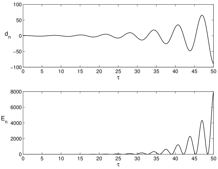
Figure 1: The temporal behavior of the normalized density $d_{n}(\tau)\equiv d(\tau)/d(0)$ and energy $E_{n}(\tau)\equiv E_{tot}(\tau)/E_{tot}(0)$ perturbations. Here, the following set of parameters was chosen: $\omega=1$, $a_{11}=-a_{22}=0.1$, $a_{12}=a_{13}=a_{21}=a_{23}=a_{31}=a_{32}=a_{33}=0$, $k_{x0}=k_{y0}=1$, $u_{x0}=u_{y0}=u_{z0}=0$, $d_{0}=0.1$.

As a first example, we consider the situation when initially only the density is perturbed. In Fig. 1 we show the temporal evolution of the density and energy perturbations normalized by their initial values. Here, the following set of parameters was chosen: $\omega=1$, $a_{11}=-a_{22}=0.1$, $a_{12}=a_{13}=a_{21}=a_{23}=a_{31}=a_{32}=a_{33}=0$, $k_{x0}=k_{y0}=1$, $u_{x0}=u_{y0}=u_{z0}=0$, $d_{0}=0.1$, Therefore, $\Gamma^{2}=0.1$ implying that the wave vector varies in time exponentially. In particular, as it is clear from the plots, for the considered time interval, $\tau\in[0-50]$, the amplitude of the density perturbations increases very rapidly from $1$ to $80$, which consequently leads to an increase of the energy of perturbations up to $\sim 8\times 10^{3}$. Generally speaking, this means that the source of the amplification of the ion sound waves is the background flow energy, which in the framework of the present approach, behaves as an infinite energy reservoir.

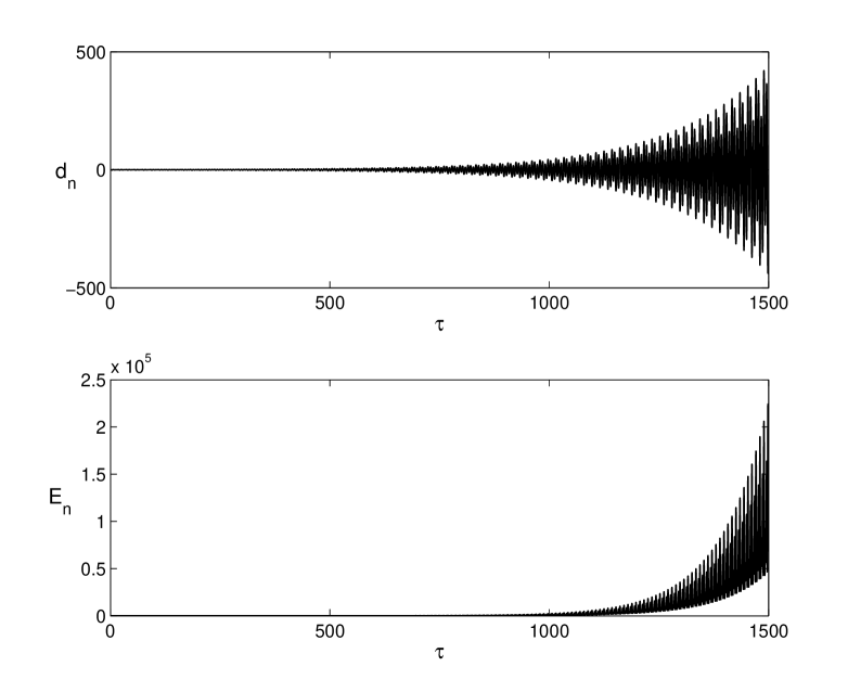
Figure 2: The temporal behavior of normalized density $d_{n}(\tau)\equiv d(\tau)/d(0)$ and energy $E_{n}(\tau)\equiv E_{tot}(\tau)/E_{tot}(0)$ perturbations. Here, the following set of parameters was chosen: $\omega=1$, $a_{12}=-0.594$, $a_{21}=0.2$, $a_{11}=a_{13}=a_{22}=a_{23}=a_{31}=a_{32}=a_{33}=0$, $k_{x0}=k_{y0}=1$, $u_{x0}=u_{y0}=u_{z0}=0$, $d_{0}=0.1$. Note that the range of $a_{12}$ where the evolution of the modes is parametrically unstable, is very narrow, viz. [-0.607; -0.580].

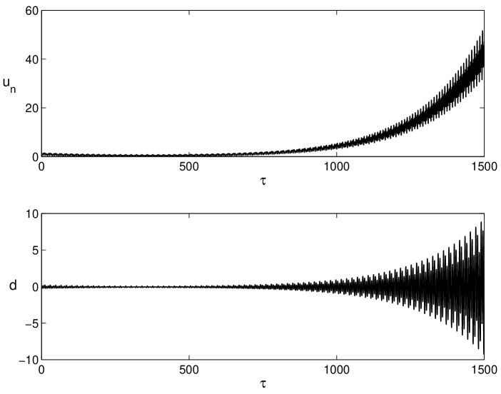
Figure 3: The temporal behavior of the normalized total velocity $u_{n}(\tau)\equiv u(\tau)/u(0)$ and density $d(\tau)$ perturbations. Here, the following set of parameters was chosen: $\omega=1$, $a_{11}=a_{13}=a_{22}=a_{23}=a_{31}=a_{32}=a_{33}$, $a_{12}=-0.594$, $a_{21}=0.2$, $k_{x0}=k_{y0}=1$, $u_{x0}=0.1$, $u_{y0}=u_{z0}=0$, $d_{0}=0$.

However, as the investigation of the shear flow dynamics shows, the system might undergo an extremely strong instability even for a negative value of $\Gamma^{2}$. For studying this particular case, we examine the following set of parameters: $a_{11}=-a_{22}=0$, $a_{12}=-0.594$, $a_{21}=0.2$, while the rest of the parameter values are the same as in the previous case. It is evident that now $\Gamma^{2}<0$ and, hence, the wave vector is characterized by periodic oscillations. In spite of this fact, the perturbations are strongly unstable. In Fig. 2 we present again the behavior of the density and energy perturbations. We see that the initially perturbed sound waves amplify very rapidly. In particular, the amplitudes of both the density and energy perturbations increase up to $\sim 540$ and $\sim 2\times 10^{5}$, respectively. It is worthwhile to note that this instability disappears if one slightly changes the parameter values. As a matter of fact, for example, if we change (increase or decrease) $a_{12}$ by no more than $\sim 2.4\%$, the system becomes stable. One can straightforwardly check that the instability takes place only when $a_{12}\in[-0.607;-0.580]$. One can thus conclude that this is, as we have anticipated, an instability of parametric nature.

In the first two examples above, we examined the evolution of some initially perturbed ion sound waves. These waves might be indirectly excited by velocity perturbations. This particular example is illustrated in Fig. 3, where the time evolution of the normalized total velocity, $u_{n}(\tau)=\sqrt{u_{x}(\tau)^{2}+u_{y}(\tau)^{2}+u_{z}(\tau)^{2}}/u_{0}$ and density is presented. Here, the following set of parameters was chosen: $\omega=1$, $a_{11}=a_{13}=a_{22}=a_{23}=a_{31}=a_{32}=a_{33}$, $a_{12}=-0.594$, $a_{21}=0.2$, $k_{x0}=k_{y0}=1$, $u_{x0}=0.1$, $u_{y0}=u_{z0}=0$, and $d_{0}=0$. One can see from the upper graph that the normalized total velocity is strongly unstable, revealing the parametric instability. Even though initially only the velocity is perturbed, we see that in due course of time, density perturbations arise as well and, correspondingly, parametrically unstable ion sound waves are generated.

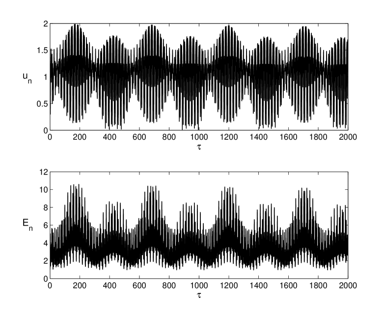
Figure 4: The temporal behavior of normalized total velocity $u_{n}(\tau)\equiv u(\tau)/u(0)$ and energy $E_{n}(\tau)$ perturbations. Here, the following set of parameters was chosen: $\omega=1$, $a_{11}=a_{13}=a_{22}=a_{23}=a_{32}=a_{33}$, $a_{12}=-0.594$, $a_{21}=0.2$, $a_{31}=-0.12$, $k_{x0}=k_{y0}=1$, $u_{x0}=0.1$, $u_{y0}=u_{z0}=0$, $d_{0}=0$.

It is well known that shear flows under favorable conditions exhibit so-called beat modes [12]. In Fig. 4, we show the behavior of both the normalized total velocity $u_{n}(\tau)\equiv u(\tau)/u(0)$ and energy $E_{n}(\tau)$ perturbations. Here, the following set of parameters was chosen: $\omega=1$, $a_{11}=a_{13}=a_{22}=a_{23}=a_{32}=a_{33}$, $a_{12}=-0.594$, $a_{21}=0.2$, $a_{31}=-0.12$, $k_{x0}=k_{y0}=1$, $u_{x0}=0.1$, $u_{y0}=u_{z0}=0$, and $d_{0}=0$. Figure 4 displays an example of such a process. From this figure we see that the ion sound wave ‘pulsates’, i.e. it is characterized by a quasi-periodic temporal “beat”. Such a structure is the result of the superposition of two frequencies that differ only by a very small amount. The fast oscillations are characterized by the ion acoustic frequency, that is modulated by a lower frequency defined by the shear parameters.

4 Conclusions

The goal of the present study was to consider ion-sound waves influenced by kinematic complexity and to study the role of the latter in the dynamical evolution of these waves. In particular, in the framework of the method developed by [10] we have considered the full set of equations, consisting of the momentum conservation equation, the mass conservation equation and the Poisson equation, and we linearized these around an equilibrium state. We have shown that, depending on the choice of the set of parameters, the system might undergo a very efficient instability. In particular, it has been found that under favorable conditions, due to the velocity shear, the wave vector becomes unstable, making the ion-sound wave strongly unstable as well. On the other hand, we have also shown an example of the excitation of acoustic modes by means of only velocity perturbations. As yet another class of instability, we have found that even when the wave vectors behave periodically, for certain ranges of the parameter values, the system becomes strongly unstable. Moreover, it has been shown that the unstable character of the ion-sound waves dramatically changes to a steady behavior by slightly changing the parameter values. Another interesting feature of the examined system is that, under certain conditions, it exhibits an ”echo”-like behavior with quasi-periodic pulsations of the ion-electrostatic modes.

In the near future, we plan to apply the developed method to realistic astrophysical flow models. In particular, it would be interesting to study the coupling of ion electrostatic waves with the velocity shear in stellar atmospheres, including young stellar objects. The idea that the ion-acoustic waves might influence the properties of stellar atmospheres has a long-standing story. For instance, in [18] the authors have considered the ion-sound waves in the solar atmosphere, studying the transition of flat solitary waves into spherical modes. One of the intriguing problems concerning solar physics is the so-called chromospheric heating, that cannot be explained only by the convective component [19]. In the framework of acoustic waves, there have been proposed several mechanisms of chromospheric heating [20, 21], but observations with Transition Region And Coronal Explorer (TRACE) NASA space telescope have shown that there is about $90\%$ deficit in the energy flux required to heat the chromosphere [22, 23, 24]. Therefore, it is interesting and quite reasonable to apply our model of kinematically driven ion-sound waves to the solar chromosphere and study the efficiency of heating.

In the present paper, we studied the fluid in a non magnetized media, although in most of the astrophysical scenarios the magnetic field plays a crucial role. Therefore, it is of fundamental importance to generalize the present work by taking into account the appearance of cyclotron modes and their possible coupling via the agency of the velocity shear with ion-sound waves.

References

References

- [1] Kerswell, R. R., 2005, Nonlinearity, 18, 17
- [2] Schekochihin, A. A., Highcock, E. G. & Cowley, S. C., 2012, PPCF, 54, 055011
- [3] Broderick, Avery E. & Loeb, Abraham, 2009, ApJ, 703, 104L
- [4] Kharb, P., Gabuzda, D. C., O’Dea, C. P., Shastri, P. & Baum, S. A., 2009, ApJ, 694, 1485
- [5] Chrysostomou, A., Bacciotti, F., Nisini, B., Ray, T. P., Eisl ffel, J., Davis, C. J. & Takami, M., 2008, A&A, 482, 575
- [6] Pike C.D., Mason H.E., 1998, Sol. Phys., 182, 333
- [7] Trefethen L.N., Trefethen A.E., Reddy S.C. Driscoll T.A., 1993, Sience, 261, 578
- [8] Criminale, W. O. & Drazin, P. G., 1990, Stud. Appl. Maths., 83, 123
- [9] Reddy, S. C. & Henningson, D. S., 1993, J. Fluid Mech., 252, 209
- [10] Lord Kelvin (W. Thomson), 1887, Phil. Mag., 24, Ser. 5, 188
- [11] Mahajan S.M., Rogava A.D., 1999, ApJ, 518, 814
- [12] Rogava A.D. & Mahajan S.M., 1997, Phys. Rev. E., 55, 1185
- [13] Rogava A.D., Mahajan S.M., Bodo G. & Massaglia S., 2003, A&A, 399, 421
- [14] Rogava A.D., Bodo G., Massaglia S. & Osmanov, Z., 2003, A&A, 408, 401
- [15] Rogava A. D., Chagelishvili, G. D. & Berezhiani V.I., 1997, Phys. Plasmas, 12, 4201
- [16] Rogava A.D., Osmanov Z. & Poedts, S., 2010, MNRAS, 404, 224
- [17] Osmanov, Z., Rogava, A. D. & Poedts, S., 2012, Phys. Plasmas 19, 012901
- [18] Edwin P. M. & Murawski K., 1995, Solar Physics, 158, 227
- [19] Judge P. G. & Carpenter K. G., 1998, ApJ, 494, 828
- [20] Lites B. W., Rutten R. J. & Kalkofen W., 1993, ApJ, 414, 345
- [21] Kalkofen W., 2007, ApJ, 671, 2154
- [22] Fossum A. & Carlsson M., 2005, ApJ, 625, 556
- [23] Fossum A. & Carlsson M., 2005, Nat, 435, 919
- [24] Fossum A. & Carlsson M., 2006, ApJ, 646, 579