RadioAstron space VLBI imaging of polarized radio emission in the high-redshift quasar 0642$+$449 at 1.6 GHz

Abstract

Context. Polarization of radio emission in extragalactic jets at a sub-milliarcsecond angular resolution holds important clues for understanding the structure of the magnetic field in the inner regions of the jets and in close vicinity of the supermassive black holes in the centers of active galaxies.

Aims. Space VLBI observations provide a unique tool for polarimetric imaging at a sub-milliarcsecond angular resolution and studying the properties of magnetic field in active galactic nuclei on scales of less than $10^{4}$ gravitational radii.

Methods. A space VLBI observation of high-redshift quasar TXS 0642$+$449 (OH 471), made at a wavelength of 18 cm (frequency of 1.6 GHz) as part of the Early Science Programme (ESP) of the RadioAstron mission, is used here to test the polarimetric performance of the orbiting Space Radio Telescope (SRT) employed by the mission, to establish a methodology for making full Stokes polarimetry with space VLBI at 1.6 GHz, and to study the polarized emission in the target object on sub-milliarcsecond scales.

Results. Polarization leakage of the SRT at 18 cm is found to be within 9% in amplitude, demonstrating the feasibility of high fidelity polarization imaging with RadioAstron at this wavelength. A polarimetric image of 0642$+$449 with a resolution of 0.8 mas (signifying an $\sim 4$ times improvement over ground VLBI observations at the same wavelength) is obtained. The image shows a compact core-jet structure with low ($\approx 2\%$) polarization and predominantly transverse magnetic field in the nuclear region. The VLBI data also uncover a complex structure of the nuclear region, with two prominent features possibly corresponding to the jet base and a strong recollimation shock. The maximum brightness temperature at the jet base can be as high as $4\times 10^{13}$ K.

1 Introduction

Very long baseline interferometry (VLBI) observations in which one of the antennas is placed on board of an Earth satellite (space VLBI) have provided a capability of reaching unprecedentedly high angular resolution of astronomical observations (Arsentev et al., 1982; Levy et al., 1986; Hirabayashi et al., 2000). The space VLBI mission RadioAstron combines ground-based radio antennas operating at frequencies 0.32, 1.6, 5, and 22 Gigahertz (GHz) with a 10-meter antenna (Space Radio Telescope, SRT) on board of the satellite Spektr-R launched on 18 July 2011 (Kardashev et al., 2013).

At 0.32, 1.6, and 22 GHz, the SRT delivers data in both left (LCP) and right (RCP) circular polarization at 0.32, 1.6, and 22 GHz, which enables fully reconstructing the linearly polarized emission from target objects at these frequencies. At 5 GHz, the SRT provides only LCP data because of a failure of the on-board hardware.

After its launch, the SRT was first tested in a single-antenna mode during the in-orbit-checkout (IOC) period (Kovalev et al., 2014) and later in the interferometry mode, in combination with ground-based antenna (fringe search, FS), successfully delivering fringes at each of the four observing bands (Kardashev et al., 2013, 2014a).

The ensuing early science program (ESP) of RadioAstron started in February 2012 and continued through June 2013 (Kardashev et al., 2014a). One of the prime objectives of the program was to provide a bridge between the initial experimental mode of operations, observing, and data processing, and routine operations that started after completion of the ESP.

One of the main goals of the ESP was to establish the feasibility of imaging experiments with RadioAstron. The first imaging experiment with RadioAstron, targeting the bright and compact radio source 0716+714, was made during the ESP period at 5 GHz (Kardashev et al., 2014a). Polarization imaging was tested with the observation presented in this paper.

Polarization imaging at high angular resolution, both along and transverse to the jet direction, is crucial for measuring the magnetic field structures of jets to distinguish between different possible magnetic field configurations. The improvement of angular resolution provided by space VLBI observations makes it particularly interesting to compare the brightness temperature and polarization measurements made with RadioAstron to the ground VLBI with a similar resolution obtained at higher observing frequencies. It has been shown that a minimum of several, independent, resolution elements across a jet are necessary to prevent spurious results from being obtained (Hovatta et al., 2012). Space VLBI observations are essential for resolving transversely a significant number of jets and studying the structure and properties of their magnetic field.

Feasibility of polarization measurements with space VLBI has been demonstrated with the VSOP (Hirabayashi et al., 2000) observations made with a satellite antenna recording data only in single (left circular) polarization (Kemball et al., 2000; Gabuzda & Gómez, 2001). Results from the first polarization observation with RadioAstron at a frequency of 1.6 GHz are reported here. This observation was made in March 2013 as part of the ESP and it targeted a bright, compact radio source TXS 0642$+$449 (OH 471).

The radio source 0642$+$449 is a distant low-polarization quasar (LPQ) located at a redshift of 3.396 (Osmer et al., 1994) which corresponds to the luminosity distance of 30.2 Gigaparsecs (Gpc) and a linear scale of 7.58 kpc/arcsecond, assuming the standard $\Lambda$CDM cosmology (Planck Collaboration et al., 2015). The optical spectrum of 0642$+$449 does not show strong broad lines (Torrealba et al., 2012). In radio, its radio structure has a compact “core–jet” morphology (Gurvits et al., 1992; Xu et al., 1995), with a flat spectral index $\alpha\approx-0.1$ (Hovatta et al., 2014) of the milliarcsecond (mas) scale core (bright narrow end of the jet).

The maximum brightness temperature, $T_{\mathrm{b}}$, measured in 0642$+$449 decreases with observing frequency. Previous VSOP space VLBI observations of 0642$+$449 at 5 GHz put a lower limit of $T_{\mathrm{b}}\geq 3.3\times 10^{12}$ K (Dodson et al., 2008), while ground VLBI observations at 15 and 86 GHz resolved the compact core and yielded somewhat lower brightness temperatures of 1.2–4.3$\,\times 10^{12}$ K (Kovalev et al., 2005) and 1.1–1.6$\,\times 10^{11}$ K (Lobanov et al., 2000; Lee et al., 2008). This implies that the compact core becomes gradually resolved out at higher frequencies, calling for comparison with the new space VLBI observations by RadioAstron.

Ground VLBI monitoring of the source has revealed a range of proper motions of 0.012–0.078 mas/yr in the jet (Lister et al., 2013) and provided estimates of the jet Lorentz factor, $\Gamma_{\mathrm{j}}=5.4$, viewing angle $\theta_{\mathrm{j}}=0.8^{\circ}$ and intrinsic opening angle $\phi_{\mathrm{j}}=0.3^{\circ}$ (Pushkarev et al., 2009). With these parameters, an equipartition magnetic field of $\approx 0.3$ G can be estimated at the location of the jet core (Lobanov, 1998) observed at 1.6 GHz, based on measurements of frequency dependent shift of the core position which have been reported for 0642+449 between frequencies of 8.1, 8.4, 12.1, and 15.4 GHz (Pushkarev et al., 2012).

Ground VLBI polarization observations at 5.0 and 8.4 GHz (O’Sullivan et al., 2011) have shown a small (1.1–2.6%) degree of polarization in the core, with no conclusive evidence for Faraday rotation ($\chi=15.6^{\circ}$ and $15.3^{\circ}$ at 5.0 and 8.4 GHz, respectively). At higher frequencies, between 8.4 and 15.1 GHz, a rotation measure (RM) of $-280$ rad/m² has been reported in the core (Hovatta et al., 2012). The Galactic RM in the direction of 0642$+$449 is estimated to be $-5.4\pm 18.3$ rad/m² (Taylor et al., 2009; Oppermann et al., 2012).

The polarization observations of 0642$+$449 with RadioAstron signal the first successful space VLBI polarization experiment using dual circular polarization measurements made at the space-borne antenna. The methodology for RadioAstron polarimetric observations and data correlation is presented in Sect. 2. The RadioAstron observation of 0642$+$449 and reduction of the polarimetric data are described in Sect. 3. The polarization image of 0642$+$449 is discussed in Sect. 4 and compared with previous ground VLBI observations of this object.

2 Imaging with RadioAstron

RadioAstron observations are performed by combining together ground-based radio telescopes with the orbiting 10-meter antenna of the SRT. The data are recorded at a rate of 128 Megabits per second, providing a total bandwidth of up to 32 MHz per circular polarization channel (Andreyanov et al., 2014). The satellite telemetry and science data are received and recorded at tracking stations in Puschino (Andreyanov et al., 2014) and Green Bank (Ford et al., 2014) and later transferred for correlation at one of the RadioAstron correlation facilities. Accurate reconstruction of the orbit and of the momentary state vector of the Spektr-R spacecraft is achieved by combining together radiometric range and radial velocity measurements made at the satellite control stations in Bear Lakes and Ussurijsk (Russia), Doppler measurements obtained at each of the tracking stations, and laser ranging and optical astrometric measurements of the spacecraft position in the sky (Khartov et al., 2014; Zakhvatkin et al., 2014). The accuracy can be further enhanced by simultaneous VLBI measurements performed on the narrow-band downlink signal from the spacecraft (Duev et al., 2012). This was demonstrated (Duev et al., 2015) using the data from the ESP observations of 0642$+$449 discussed here.

The Spektr-R satellite has a highly elliptical orbit, with the apogee reaching up to 350,000 km and the perigee varying in the 7,000–80,000 km range. The orbital period of the satellite varies between 8.3 and 9.0 days (Kardashev et al., 2013, 2014b). These factors make imaging observations with RadioAstron particularly challenging, with optimal conditions realized typically only for a limited fraction of sky and for limited periods of time. The imaging observations are planned by simulating the observing conditions in the FakeRaT software package (Zhuravlev, 2014), which is based on the FakeSat software (Murphy, 1991; Murphy et al., 1994).

The Fourier spacings provided by the ground-space baselines to the SRT are typically limited to a very narrow range of position angle and often does not reach down to the spacings of the baselines between ground-based telescopes. In order to reduce the adverse effect of these two factors, imaging with RadioAstron is performed during the perigee passages of the SRT (perigee imaging), typically with 12-24 hour-long observing segments. Whenever feasible, these perigee imaging segments are augmented by several 1-2 hour-long segments (long-baseline tracking) allocated during the following days and including a smaller number (3-4) of ground antennas. The long-baseline tracking provides information on largest Fourier spacings, enabling detecting the emission on the finest angular scales.

2.1 Correlation of RadioAstron experiments

Correlation of RadioAstron experiments is performed at three different correlator facilities: the ASC RadioAstron correlator (Kardashev et al., 2013; Andrianov et al., 2014), the JIVE SFXC correlator (Kettenis, 2010), and the DiFX software correlator (Deller et al., 2007, 2011). In order to enable the correlation of RadioAstron data to be made in the DiFX correlator, the DiFX code has been upgraded by the Max-Planck-Institute for Radio Astronomy (MPIfR) in Bonn, addressing the specific aspects of data and telemetry formats of the SRT telescope on-board the Spektr-R spacecraft (Bruni, 2014; Bruni et al., 2015).

The upgrade has comprised a new routine to read the native RadioAstron Data Format (RDF) into the DiFX correlator and a number of modifications to the correlator code enabling it to process data recorded at the SRT. The delay model server CALC from the CALC/SOLVE package used by the DiFX correlator is modified to be able to calculate delay information for telescopes with arbitrary coordinates and velocities, accounting for the general relativistic effects in the gravitational field of the Earth. The DiFX metadata system is upgraded to deal with the changing position and velocity of the spacecraft as a function of time.

Satellite orientation parameters provided in the telemetry are used in the upgraded version of the code for calculating the equivalent of parallactic angle correction for the spaceborne antenna. The estimated accuracy of the orientation parameters is $\approx 1^{\prime\prime}$ (Lisakov et al., 2014). This enables accurate calibration of the instrumental polarization of the SRT.

The timestamps for the SRT data (set by the tracking station clock at the moment it begins recording individual VLBI scans) are modified to refer to the relative time of arrival of the astronomical signal at the spacecraft. This is done by calculating the delay for the transmission of the signal from the spacecraft to the tracking station. These corrections are inserted to the metadata handler and to the delay model server, which provides the full compatibility of the RadioAstron data stream with data streams from ground antennas.

The upgraded DiFX correlator is now used at the MPIfR to correlate RadioAstron data and being prepared for merging with the trunk version of the DiFX correlator code.

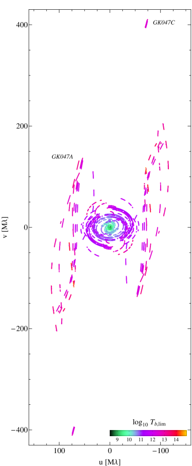
Figure 1: Coverage of the Fourier domain (uv coverage) of the RadioAstron observation of 0642$+$449 at 1.6 GHz ($\lambda=18$ cm), plotted in units of M$\lambda$. The central part corresponds to the perigee imaging segment (GK047A) and the short segment at $v\approx 400$ M$\lambda$ represents the long-baseline tracking segment (GK047C). Color marks the upper limit of brightness temperature obtained from visibility amplitudes (for details, see discussion in Sect. 4.1).

Table 1: Radio telescopes participating in RadioAstron observation of 0642$+$449

Telescope		$D$	SEFD	Observing time [UT]		$B_{\mathrm{max}}$
	Code	[m]	[Jy]	GK047A	GK047C	[$D_{\mathrm{E}}$]
Spektr-R SRT (RU)	RA	10	2840	10:00 – 01:00	14:00 – 15:00	…
Effelsberg (DE)	EF	100	19	10:00 – 01:00	14:00 – 15:00	5.87
Jodrell Bank (UK)	JB	76	65	10:00 – 01:00	14:50 – 15:00	5.93
WSRT (NL)	WB	66†	40	13:00 – 01:00	14:00 – 15:00	5.90
Torun (PL)	TR	32	300	10:00 – 01:00		2.76
Urumqi (CH)	UR	25	300	10:00 – 23:00		3.02
Shanghai (CH)	SH	65	670	10:00 – 19:00		3.26
Noto (I)	NT	32	784	10:30 – 01:00		2.69
Hartebeesthoek (SA)	HH	26	430	14:30 – 20:00		1.91
Green Bank (USA)	GB	100†	10	17:00 – 01:00		1.63
Zelenchukskaya (RU)	ZC	32	300	19:30 – 23:30		1.67

Notes: $D$ – antenna diameter (${\dagger}$ – equivalent diameter); SEFD – system equivalent flux density (system noise), describing the antenna sensitivity; $B_{\mathrm{max}}$ – largest projected baseline in the data, in units of the Earth diameter.

3 RadioAstron observation of 0642$+$449

The 1.6 GHz RadioAstron observation of 0642$+$449 (RadioAstron project code raes12; global VLBI project code GK047) was made on 9-10 March 2013, with three observing segments allocated for the experiment. The main perigee imaging segment, GK047A (raes12a; 10:00 UT/09/03–01:00 UT/10/03) was complemented by VLBI observations of the satellite downlink signal at 8.4 GHz (segment GK047B) made for the purpose of improving the Spektr-R orbit determination (Duev et al., 2015). The third segment, GK047C (raes12b; 14:00 UT/10/03–15:00 UT/10/03) was introduced as a long-baseline tracking segment. The SRT data and the satellite telemetry were recorded by the RadioAstron satellite tracking station in Puschino. Basic parameters of the ground telescopes participating in the segments GK047A and GK047C are given in Table 1.

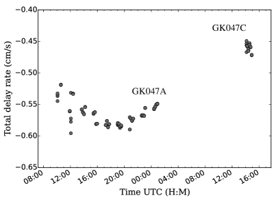
Figure 2: Total delay rates of the SRT obtained from baseline-based fringe fitting of the correlated data on the baseline to Effelsberg and accounting for the clock rates at each of the two telescopes. For each SRT observing segment, the rates are obtained from fringe fitting solutions with a time interval of 10 minutes. The rates are plotted separately for each IF and polarization channels. The plot reflects the accuracy of the velocity determination in the reconstructed orbit of the SRT. All of the velocity and acceleration values correspond to the baseline projections of the true residual offset, velocity, and acceleration of the spacecraft.

The data were recorded in two polarization channels (left and right circularly polarized, LCP and RCP), with a bandwidth of 32 MHz per channel, centered at a frequency of 1.6601875 GHz. In each of the channels, the total bandwidth was split into two independent intermediate frequency (IF) bands of 16 MHz.

The space VLBI segments on 0642$+$449 were observed in a 40/120 minute on/off cycle, with the gaps between the segments required for cooling the motor drive of the on-board high-gain antenna of the Spektr-R. During these gaps, the strong radio sources 1328+207 (3C 286) and 0851+202 (OJ 287) were also observed with the ground antennas as polarization calibrators. Fig. 1 shows the resulting visibility coverage of the Fourier domain (uv coverage, expressed in units of spatial frequency defined as a ratio of instantaneous projected baseline length to the observing wavelength, $\lambda$) of the data recorded for 0642$+$449.

3.1 Data correlation

The data correlation was performed at the DiFX software correlator of the MPIfR. Fringe search for RadioAstron was performed for every scan, and ad-hoc values for delay offsets and rates were determined and applied, in order to compensate for the acceleration terms of the spacecraft. The initial fringe-search was performed with 1024 spectral channels per IF and an integration time of 0.1 sec (providing respective search ranges of 10 microseconds and 10^-9 sec/sec for the delay and the delay rate), in order to accommodate for potential large residual delays at the SRT. Fringes between the SRT and the reference antenna of Effelsberg were found with a residual delay offset of only about 1 microsecond or less, and a delay rate of about 2$\times$10^-11 sec/sec (60 cm/s). The fringe solutions for the SRT were typically found at high signal-to-noise ratio (SNR): all but three scans showed fringes with SNR$>$10. For the three scans with low SNR, values of delay offset and rate were interpolated from adjacent scans. Final correlation was performed with 32 spectral channels per IF (with the corresponding channel width of 500 kHz) and 0.5 sec of integration time.

Figure 3: Bandpass amplitudes and phases on ground-space baselines between the SRT and Effelsberg (top two rows) and Urumqi (bottom two rows), after applying global fringe fitting solutions. The bandpasses for total intensity (parallel hands: LL, RR) and polarized emission (cross-hands: LR, RL) are shown.

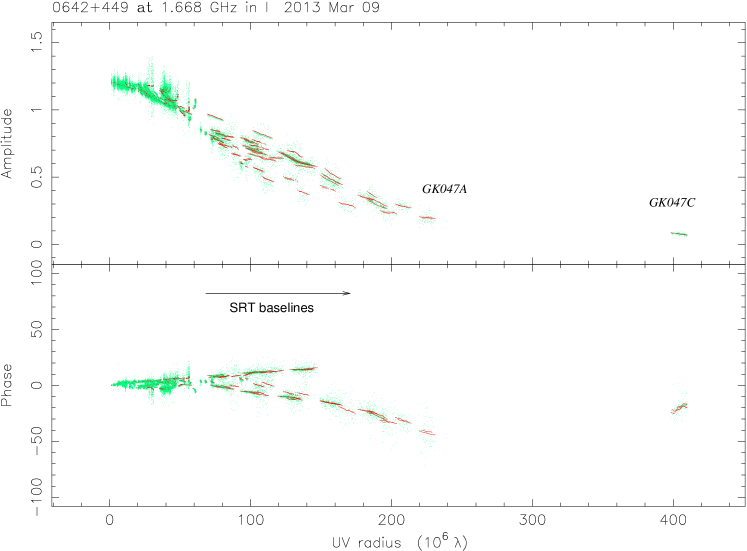
Figure 4: Visibility amplitude (top) and phase (bottom) distributions as a function of uv radius, overplotted with the CLEAN model (red color) obtained during the hybrid imaging of the source structure.

3.2 Post-correlation data reduction

The correlated data were reduced in several steps using AIPS and Difmap (Shepherd, 1997, 2011). The initial calibration was performed in AIPS, imaging was done using Difmap, and both packages were used for calibrating the instrumental polarization and providing absolute calibration of the polarization vectors. The segments GK047A and GK047C were calibrated independently and combined together for the final imaging. Polarization calibration was performed using the segment GK047A (the parallactic angle coverage of GK047C was insufficient for using this segment for the polarization calibration).

The a priori amplitude calibration was applied using the default antenna gains and the system temperature measurements made at each antenna during the observation. For the SRT, the sensitivity parameters measured during the IOC (Kovalev et al., 2014) were used. The data were edited using the flagging information from the station log data. Parallactic angle correction was applied, to correct for feed rotation with respect to the target sources.

3.2.1 Fringe fitting

The data were fringe fitted in two steps, first by applying manual phase-cal corrections and then using the global fringe search for antenna rates and single and multi-band delays. The group delay difference between the two polarization channels was corrected. The resulting post-fringe residual delay rates obtained for the SRT are plotted in Fig. 2. These slowly evolving residuals agree well with the expected accuracy of the orbital velocity determination for the SRT (Kardashev et al., 2013), but they still should be viewed only as an indicator of the fidelity of the fringe fitted data, while a more detailed discussion of the accuracy of the orbit determination for the SRT is presented elsewhere (Duev et al., 2015).

3.2.2 Bandpass calibration

After the fringe fitting, the receiver bandpasses were corrected. The bandpass-calibrated data on the baselines between the SRT and the ground antennas in Effelsberg and Urumqi is shown in Fig. 3. The interferometric visibility signal is clearly detected both in the total intensity (LL and RR) and the cross-polarization (LR and RL) channels, demonstrating the excellent quality of the data. Table 2 lists typical amplitude and phase errors of the visibility data on the longest baselines to the SRT observed in the segment GK047A, demonstrating that the source was detected on baselines to all participating antennas (the errors were calculated by vector averaging the calibrated data over two IFs and over a scan length of 10 minutes, and hence these errors are conservative estimates containing also contributions from residual bandpasses and offsets between the IFs, and from amplitude and phase variations over the scan time).

Table 2: Typical amplitude and phase errors on the baselines to the SRT

Ant.	Polarization
Code	LL,RR		LR,RL
	$\sigma_{\mathrm{amp}}$	$\sigma_{\mathrm{ph}}$	$\sigma_{\mathrm{amp}}$	$\sigma_{\mathrm{ph}}$
	[%]	[∘]	[%]	[∘]
EF	5.5	2.9	22.6	50.2
JB	9.3	3.0	30.7	51.9
WB	6.0	3.1	30.5	46.8
TR	11.6	4.6	38.3	54.2
UR	13.6	6.5	45.0	60.5
SH	53.9	56.6	53.9	84.6
NT	18.3	9.3	54.1	80.0
HH	52.8	65.1	50.8	67.2
GB	6.5	2.6	33.4	42.7
ZC	25.1	13.8	50.6	57.7

Notes: Columns represent average fractional amplitude, $\sigma_{\mathrm{amp}}$ and phase, $\sigma_{\mathrm{ph}}$, errors of the total (LL, RR) and cross-polarized (LR, RL) correlated flux density detected on the SRT baselines to the ground radio telescopes.

Table 3: Instrumental polarization (D-terms)

Antenna	RCP		LCP
	$m$	$\chi$	$m$	$\chi$
	[%]	[∘]	[%]	[∘]
RA	6.8$\pm$0.3	82$\pm$6	8.2$\pm$0.8	98$\pm$1
	7.0$\pm$0.2	81$\pm$8	8.7$\pm$0.9	98$\pm$2
EF	2.6$\pm$0.3	10$\pm$2	2.3$\pm$0.1	167$\pm$9
	3.1$\pm$0.3	8$\pm$3	2.4$\pm$0.1	185$\pm$9
JB	1.3$\pm$0.4	140$\pm$7	3.5$\pm$0.6	336$\pm$3
	0.8$\pm$0.4	306$\pm$7	4.3$\pm$0.6	330$\pm$3
WB	4.6$\pm$0.5	176$\pm$3	2.5$\pm$0.2	166$\pm$13
	4.6$\pm$0.9	182$\pm$3	2.4$\pm$0.4	199$\pm$12
TR	8.0$\pm$0.5	160$\pm$3	7.2$\pm$0.6	14$\pm$8
	8.7$\pm$0.4	164$\pm$3	7.6$\pm$0.3	31$\pm$8
UR	11.6$\pm$1.0	271$\pm$12	10.2$\pm$1.1	56$\pm$18
	12.5$\pm$1.1	294$\pm$12	12.2$\pm$1.2	93$\pm$18
SH	6.3$\pm$0.5	173$\pm$31	5.5$\pm$0.4	13$\pm$30
	6.3$\pm$1.0	170$\pm$32	4.5$\pm$0.8	349$\pm$30
NT	5.8$\pm$0.3	247$\pm$5	5.9$\pm$0.2	239$\pm$6
	5.3$\pm$0.2	184$\pm$5	5.4$\pm$0.2	178$\pm$8
HH	21.7$\pm$1.8	151$\pm$23	19.9$\pm$5.2	80$\pm$35
	18.1$\pm$1.8	198$\pm$23	9.5$\pm$5.2	149$\pm$35
GB	5.4$\pm$0.3	248$\pm$6	5.1$\pm$0.8	295$\pm$10
	4.8$\pm$0.3	236$\pm$6	3.5$\pm$0.8	315$\pm$10
ZC	8.0$\pm$0.7	160$\pm$7	5.2$\pm$1.0	146$\pm$3
	9.5$\pm$0.7	146$\pm$7	7.2$\pm$1.0	141$\pm$3

Notes: For each antenna, listed are the fractional amplitude, $m$, and phase, $\chi$, of the instrumental polarization (polarization leakage) in the right (RCP) and left (LCP) circular polarization channel and in the first (IF1, top row) and second (IF2, bottom row) intermediate frequency channel. The D-term phases have been corrected for the phase offsets obtained from the EVPA calibration described in Sect. 3.2.4.

3.2.3 Polarization calibration

After applying the bandpass calibration, the calibrated Stokes I data were exported to Difmap and imaged using hybrid imaging with CLEAN deconvolution and self-calibration (with full phase self-calibration and limited amplitude calibration using a single amplitude gain correction per antenna). The resulting self-calibrated visibility amplitudes and phases (and their CLEAN model representations) are shown in Fig. 4 for all of the baselines as a function of Fourier spacing (uv distance). The visibilities indicate that the source structure is clearly detected up to the longest ground-space baselines of the observation.

The polarization calibration proceeded then with the self-calibrated model of the source structure obtained. The model was imported into AIPS and used as the calibration model for the full Stokes data, with amplitude and phase calibration applied on time intervals of 1 minute.

The instrumental polarization (polarization leakage terms or D-terms, comprising the fractional amplitude and phase) was obtained using the LPCAL method (Leppanen et al., 1995), with Effelsberg used as the reference antenna. The resulting polarization leakages determined through this procedure are listed in Table 3. Errors of the D-terms were estimated from averaging the respective values determined for each of the calibrators and for the target itself. To estimate the errors for the SRT (which did not observe the calibrators), the D-terms obtained from each of the calibrators with the ground antennas were applied to the data on 0642$+$449 and respective solutions for the D-terms of the SRT were obtained and compared with the solution obtained directly from the target data (hence the D-terms errors for the SRT might be underestimated). The amplitude of instrumental polarization of the SRT is found to be within 9% and with excellent phase consistency between the IFs. This figure cannot be directly compared with the results from pre-launch measurements, as those measurements were made only for the antenna feeds of the SRT, yielding an $\approx 2$% leakage at 1.6 GHz (Turygin, 2014). The polarization leakage of the SRT is comparable to the instrumental polarization obtained for the ground antennas, demonstrating robust polarization performance of the SRT and ensuring reliable polarization measurements with data on all ground-space baselines. Similar estimates of the L-band polarization leakage were obtained for the SRT from the analysis of the RadioAstron AGN survey observations (Pashchenko et al., 2015).

Table 4: Effelsberg measurements of total and polarized flux densities of the targets

Source	$S_{\mathrm{tot}}$	$S_{\mathrm{pol}}$	$\chi$
	[Jy]	[Jy]	[deg]
0642+449	$\leavevmode\nobreak\ 1.32\pm 0.02$	$0.022\pm 0.008$	$77.2\pm 12.0$
0851+202	$\leavevmode\nobreak\ 2.77\pm 0.03$	$0.069\pm 0.016$	$32.1\pm\leavevmode\nobreak\ \leavevmode\nobreak\ 1.7$
1328+307	$13.68\pm 0.21$	$1.37\pm 0.10\leavevmode\nobreak\ \leavevmode\nobreak\$	$33.3\pm\leavevmode\nobreak\ \leavevmode\nobreak\ 1.4$

Notes: Measurements were made on 9-10 March 2013. Column designation: $S_{\mathrm{tot}}$ – total flux density; $S_{\mathrm{pol}}$ – polarized flux density; $m$ – percentage of polarization; $\chi$ – position angle of the electric vector position angle (EVPA).

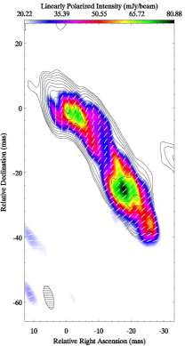
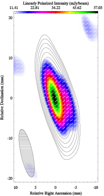
Figure 5: Ground array images of the calibrator sources 1328$+$307 (left) and 0851$+$202 (right), made using the uniform data weighting. Image parameters are listed in Table 5. Contours show the total intensity; colors indicate linearly polarized intensity; vectors show the EVPA orientation.

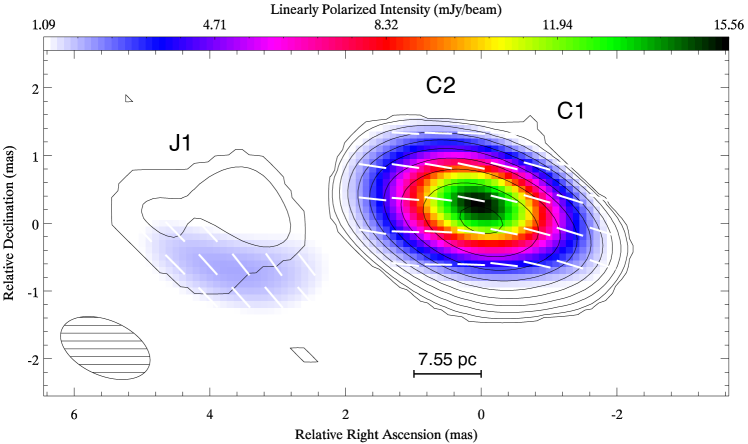
Figure 6: RadioAstron space VLBI image of 0642$+$449 of total (contours) and linearly polarized (color shades) emission, made using the uniform data weighting. The orientation of linear polarization is indicated by vectors. Basic parameters of the total intensity image are listed in Table 5. Labels indicate the modelfit decomposition of the source structure described in Table 6.

After applying the D-terms determined for the SRT and the ground antennas, the calibrated full Stokes data were exported into Difmap, imaged in Stokes I, Q, and U, and combined together, providing images of the total intensity, linearly polarized intensity, and polarization vectors (electric vector position angle, EVPA).

3.2.4 EVPA calibration

The absolute EVPA calibration was performed using single-dish measurements of the total flux density polarization of the target and calibrator sources. These measurements (listed in Table 4) were made concurrently with the RadioAstron observation at the Effelsberg 100-meter telescope. The averaged EVPA of the polarized emission detected in the VLBI data was related to the polarization vectors that were measured with the Effelsberg antenna, and the resulting EVPA offsets were applied to the VLBI images. The resulting ground array images of the calibrator sources are shown in Fig. 5, and the image parameters are listed in Table 5.

4 Polarization image of 0642$+$449

The RadioAstron polarization image of 0642$+$449 is shown in Fig. 6, and the basic parameters of the image are listed in Table 5. The source shows a compact core-dominated structure, with a resolved nuclear region which contains about 98% of the total flux density in the image. The weak and extended jet feature, J1, located at about 4 mas separation from the nucleus has a peak brightness of $\approx 15$ mJy/beam, which is not surprising considering energy losses due to adiabatic expansion of the flow up to the estimated deprojected linear separation of 2.3 kpc of this feature from the core of the source (assuming the jet viewing angle of 0.8^∘; Pushkarev et al. 2009). The linear separation can be a factor of $\sim 3.5$ smaller, if the observed misalignment of $\approx 2^{\circ}$ between the position angles of C2 and J1 reflects the physical change of the jet direction. The observed concentration of the polarized flux density along the southern edge of this feature may reflect interaction with the ambient medium occurring in this region, although it may also result from the errors of the D-terms determination or from other instrumental effects (cf. Gabuzda & Gómez, 2001; Hovatta et al., 2012).

Table 5: Parameters of total intensity images

Source	$S_{\mathrm{tot}}$	$S_{\mathrm{peak}}$	$S_{\mathrm{neg}}$	$\sigma_{\mathrm{rms}}$	Beam
0851$+$202	2.06	1.73	-19.0	6.5	12.2,2.93,12.6
1328$+$307	7.87	0.89	-47.1	8.6	7.48,2.73,14.9
0642$+$449	1.21	0.81	3.6	0.7	1.38,0.81,66.5

Notes: Column designation: $S_{\mathrm{tot}}$ [Jy] – total flux density; $S_{\mathrm{peak}}$ [Jy/beam] – peak flux density; $S_{\mathrm{neg}}$ [mJy/beam] – maximum negative flux density in the image; $\sigma_{\mathrm{rms}}$ [mJy/beam] – rms noise in the image; Beam: major axis, minor axis, position angle of major axis [mas, mas, ^∘].

Table 6: Decomposition of compact structure in 0642$+$449

Comp.	$S_{\mathrm{tot}}$	$r$	$\phi$	$\theta$	$\theta_{\mathrm{min}}$	$T_{\mathrm{b}}$	$S_{\mathrm{pol}}$	$m_{\mathrm{pol}}$	$\chi_{\mathrm{pol}}$
	[mJy]	[mas]	[∘]	[mas]	[mas]	[1011 K]	[mJy]	[%]	[∘]
C1	462$\pm$16	0.38$\pm$0.01	$-$88.3$\pm$0.7	0.40$\pm$0.01	0.16	12.8$\pm$0.6	7.7$\pm$0.8	1.7$\pm$0.2	79$\pm$3
C2	721$\pm$19	0.32$\pm$0.01	70.1$\pm$1.1	0.60$\pm$0.01	0.13	8.8$\pm$0.3	9.9$\pm$0.7	1.4$\pm$0.1	89$\pm$2
J1	20$\pm$9	3.80$\pm$0.20	92.0$\pm$3.2	0.89$\pm$0.43	0.75	0.11$\pm$0.04	1.7$\pm$0.7	8.5$\pm$5.2	39$\pm$11

Notes: Gaussian model description: $S_{\mathrm{tot}}$ – total flux density; component position in polar coordinates ($r,\,\phi$) with respect to the map center; component size, $\theta$; minimum resolvable size, $\theta_{\mathrm{min}}$, of the respective component; brightness temperature, $T_{\mathrm{b}}$, in the observer’s frame, derived for the parameters of the Gaussian fit. Polarization properties (measured from the Stokes U and Q images: $S_{\mathrm{pol}}$ – flux density of linearly polarized emission; $m_{\mathrm{pol}}$ – fractional polarization; $\chi_{\mathrm{pol}}$ – polarization position angle in the sky plane (measured North-through-East).

The core region is clearly resolved and extended along a P.A. of $\approx 81^{\circ}$, It can be decomposed into two circular Gaussian components. The resulting three-component decomposition of the source structure is presented in Table 6. The two nuclear components, C1 and C2, are separated by 0.76 mas ($\approx 410$ pc, deprojected). Similar structural composition of the nuclear region is also detected in the ground VLBI from the MOJAVE survey at 15 GHz (Lister et al., 2013). The same structure is also present in the images of 0642$+$449 made at 24 and 43 GHz (Fey et al., 2000).

Overall, the structure observed in 0642$+$449 may be similar to the main features of the jet in M 87 (cf. Sparks et al., 1996), in which a prominent standing shock (component HST-1) is located at 200–280 pc (considering the uncertainty of the jet viewing angle) and a prominent feature A located at 2.8–3.7 kpc distance from the core is believed either to be an oblique shock (Bicknell & Begelman, 1996) or to result from the helical mode of Kelvin-Helmholtz instability (Lobanov et al., 2003). This may also explain the apparent displacement between the total intensity and linearly polarized emission in the region J1, which is similar to the polarization asymmetries observed in M 87 at these linear scales (Owen et al., 1989).

The polarized emission detected in 0642$+$449 is dominated by the two nuclear components, with fractional polarization reaching 15.6 mJy ($\approx 2$%), and the magnetic field showing predominantly transverse orientation with respect to the general jet direction (assuming that the innermost component C1 corresponds to the canonical “VLBI core” region in which the emission becomes optically thin at the frequency of observation; Konigl 1981). The polarization vectors vary by about $10^{\circ}$ across the nucleus, with the polarization angle observed in the most compact region C1 ($\approx 80^{\circ}$) coming close to the polarization angle measured with Effelsberg. A substantial rotation of the EVPA vectors is seen in some of the MOJAVE images of 0642$+$449, which is likely to result from plasma propagation in a jet observed at an extremely small viewing angle. The weak ($\sim 2$ mJy/beam) linearly polarized emission in the jet component J1 corresponds to a fractional polarization of $\sim 15$%, with a large error margin on this estimate. The magnetic field is roughly longitudinal in this region.

The MOJAVE database lists, for the frequency of 15 GHz, an EVPA of 122^∘ in March 2011. Analysis of the multifrequency MOJAVE observations (Hovatta et al., 2012) yields, for 0642$+$449, a median rotation measure of $-268$ rad/m² over the whole source structure, with a slightly higher rotation measure of $-280$ rad/m² over the compact core region.

Assuming a linear trend in the EVPA in time as derived from the two latest MOJAVE observations, the polarization angle should be $\sim 105^{\circ}$ in March 2013 at 15 GHz. We measure $\chi=80^{\circ}$–90^∘ over the core region. Formally, this corresponds to a rotation measure of $-15$ rad/m², under assumption that the rotation measure is not affected by the core shift. It would then require about three turns of phase to get this value to be reconciled with the RM reported from the MOJAVE measurements. Alternatively, the smaller RM estimated from the RadioAstron measurements may reflect the reported trend of decreasing RM with decreasing frequency (Kravchenko et al., 2015). It would still require about one turn of phase to bring the estimated RM value to a better agreement with the empirical dependence $|\mathrm{RM}|(\nu)\propto\nu^{1.6}$ derived in Kravchenko et al. (2015).

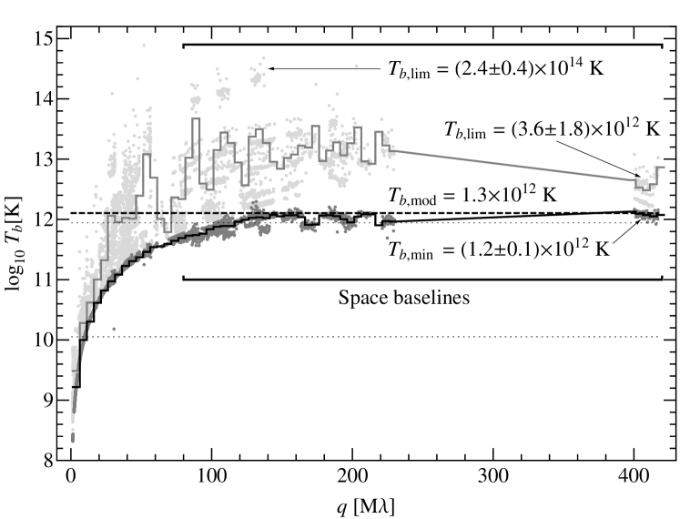
Figure 7: Visibility-based estimates of the brightness temperature in 0642$+$449, calculated in the observer’s frame. Data points represent the minimum (dark gray), $T_{\mathrm{b,min}}$, and maximum limiting (light gray), $T_{\mathrm{b,lim}}$, brightness temperatures derived from individual visibilities measured at different uv distances, $q$ (Lobanov, 2015). The two-dimensional distribution of $T_{\mathrm{b,lim}}$ is also presented in Fig. 1 with a color wedge. Braces above and below the brightness temperature data indicate the range of uv distances covered by the space baselines of the RadioAstron observation. The histograms show the respective brightness temperatures averaged over bins of 5 M$\lambda$ in size. The thick dashed line indicates the brightness temperature, $T_{\mathrm{b,mod}}=1.3\times 10^{12}$ K, derived for the most compact feature, C1, of the Gaussian fit of the source structure described in Table 6. The dotted lines indicate the respective brightness temperatures of the other two Gaussian components. The minimum brightness temperature, $T_{\mathrm{b,min}}=1.2\times 10^{12}$ K, is constrained by the visibilities with $q>380$ M$\lambda$. The maximum limiting brightness temperature $T_{\mathrm{b,lim}}=2.4\times 10^{14}$ K can be estimated from the data on the SRT baselines to Noto and Hartebeesthoek, although potential problems with amplitude calibration cannot be ruled out. A more conservative estimate of $T_{\mathrm{b,lim}}=3.6\times 10^{12}$ K can be obtained from the data on the longest space-ground baselines.

4.1 Brightness temperature

The Gaussian modelfit described in Table 6 can be used for obtaining estimates of brightness temperature (also presented in the same Table), with the highest brightness temperature of $1.3\times 10^{12}$ K associated with the most compact core feature C1. This value is somewhat lower than the one that should be expected at 1.6 GHz, based on the trend $\log_{10}T_{\mathrm{b}}[\mathrm{K}]=13.3-1.1\,\log_{10}\nu[\mathrm{GHz}]$ that can be obtained from the existing measurements at 5, 15, and 86  GHz (Lobanov et al., 2000; Kovalev et al., 2005; Dodson et al., 2008; Lee et al., 2008). However, since the morphology of the emitting region can be different from a simple Gaussian shape, the actual brightness temperature of the emission may differ from the modelfit-based estimates, for instance, if the brightness distribution is smooth and the respective brightness temperature is largely determined mostly by the transverse dimension of the flow (Lobanov, 2015). To investigate this possibility, the modelfit-based estimates of $T_{\mathrm{b}}$ can be compared with estimates obtained directly from visibility amplitudes and their errors, which yields the absolute minimum brightness temperature, $T_{\mathrm{b,min}}$, and an estimate of the limiting brightness temperature, $T_{\mathrm{b,lim}}$ that can obtained from the data under the requirements that the structural detail sampled by the given visibility is resolved (Lobanov, 2015).

These two estimates are compared in Fig. 7 with the brightness temperatures calculated from the Gaussian modelfit. This comparison shows that the visibility amplitudes on the space baselines longer that $\approx 140$ M$\lambda$ require the brightness temperature to be larger than $10^{12}$ K, which agrees with $T_{\mathrm{b}}$ obtained for the most compact feature C1 of the Gaussian modelfit. The limiting brightness temperature $T_{\mathrm{b,lim}}=3.6\times 10^{12}$ K can be estimated at the longest space baselines. These visibilities concentrate however only within a narrow range of position angles ($-10\mbox{$.\!\!^{\circ}$}2\pm 0\mbox{$.\!\!^{\circ}$}1$), with corresponding structural sensitivity limited to ${\mathrm{P}.A.}\approx 80^{\circ}$, which essentially coincides with direction of the inner jet (hence resulting in lower visibility amplitudes and, consequently, lower estimates of $T_{\mathrm{b,lim}}$).

Indeed, some of the $T_{\mathrm{b,lim}}$ estimated from the visibility amplitudes at shorter space baselines and different position angles reach above $10^{14}$ K, notably with a large spread of the estimates obtained at similar spatial frequencies. The observed spread reflects the difference of signal-to-noise ratios (SNR) in the measurements on different baselines, and it also may indicate potential biases due to a priori gain calibration and amplitude self-calibration. The three particularly outstanding clusters of points in Fig. 7, which have $T_{\mathrm{b,lim}}>10^{14}$ K, come from visibilities on the baselines to Westerbork, Torun, Noto, and Hartebeesthoek.

As the visibility SNR on these baselines is typically lower than on baselines to Effelsberg or Jodrell Bank (which do not yield such high $T_{\mathrm{b,lim}}$ at similar radial distances and position angles), it is most likely that the exceptionally high brightness temperature limits are caused by problems with the amplitude calibration of the antenna gains or specific observing scans with these antennas.

If the outliers are ignored and only the bulk of the $T_{\mathrm{b,lim}}$ estimates are considered in the range of 100–200 M$\lambda$, the average $T_{\mathrm{b,lim}}$ increases to $9.1\times 10^{12}$ K, and this can be viewed as a viable upper limit on the brightness temperature of the most compact structure in the jet of 0642$+$449. This corresponds to brightness temperature of $4.0\times 10^{13}$ K in the rest frame of the source. If the brightness temperature is generally determined by the transverse dimension of the flow, as suggested by the analysis of the MOJAVE visibility data (Lobanov, 2015), the inner jet of 0642$+$449 should have a width of $\approx 0.15$ mas to satisfy the limiting brightness temperature estimated above.

5 Summary

The RadioAstron Early Science observations of the high-redshift quasar TXS 0642$+$449 have tested the polarization performance of the space radio telescope (SRT) at 1.6 GHz ($\lambda=18$ cm) and provided a framework for establishing a set of procedures for correlation, post-processing and calibration of space VLBI polarization data. The instrumental polarization of the SRT is found to be less than 9%, which enables robust reconstruction of the polarization signal on the ground-space baselines of RadioAstron observations and provides a basis for high-fidelity imaging of polarized emission.

The total and linearly polarized emission from the quasar 0642$+$449 is detected on the SRT baselines of up to 75,560 km (5.93 Earth diameters) in length, corresponding to angular scales of 0.5 milliarcseconds (mas). The resulting RadioAstron image of linearly polarized emission in 0642$+$449 has a resolution of 0.8 mas, which is $\sim 4$ times better than the resolution of ground VLBI images at 18 cm. The image probes the physical conditions in the jet on angular scales as small as $\approx 0.2$ mas (linear scale of $\approx 1.5$ pc) taking into account the SNR-driven resolution limits of the observation.

The structure of total intensity and linearly polarized emission recovered from the RadioAstron image of 0642$+$449 suggests that this object is likely to be a “canonical” quasar with a powerful relativistic jet observed at an extremely small angle of sight and featuring a bright “core” of the jet (component C1) and a likely recollimation shock (component C2) located at a deprojected distance of about 400 pc away from the core. Each of these regions is only weakly polarized, with fractional polarization not exceeding $\approx 2\%$ and polarization vector implying a predominantly transverse magnetic field (in agreement with expectations for strong shocks in jet). The weak and more distant feature J1 observed at a separation of $\approx 3.8$ mas ($\approx 2$ kpc, deprojected) has a much stronger polarization, possibly exceeding a 10% level. The dominant magnetic field components is likely to be poloidal in this region, implying that it either represents a weak shock or may even result from plasma instability developing in the jet.

The RadioAstron data have also been used for making brightness temperature measurements based on the Gaussian decomposition (modelfit) of the structure and on estimates made directly from the visibility data. The most robust estimate provided by these measurements yields a brightness temperature of $\approx 3.6\times 10^{12}$ K for the most compact region in the jet. Further analysis of the RadioAstron data indicate that the the brightness temperature of the radio emission from this region cannot be lower that $\sim 10^{12}$ K and is not likely to exceed $\approx 9\times 10^{12}$ K (corresponding to $\approx 4\times 10^{13}$ K in the reference frame of the source).

References

- Andreyanov et al. (2014) Andreyanov, V. V., Kardashev, N. S., & Khartov, V. V. 2014, Cosmic Research, 52, 319
- Andrianov et al. (2014) Andrianov, A. S., Girin, I. A., Zharov, V. E., et al. 2014, Proc. of S.A. Lavochkin Association, 3, 55
- Arsentev et al. (1982) Arsentev, V. M., Berzhatyi, V. I., Blagov, V. D., et al. 1982, Akademiia Nauk SSSR Doklady, 264, 588
- Bicknell & Begelman (1996) Bicknell, G. V. & Begelman, M. C. 1996, ApJ, 467, 597
- Bruni (2014) Bruni, G. 2014, in COSPAR Meeting, Vol. 40, 40th COSPAR Scientific Assembly. Held 2-10 August 2014, in Moscow, Russia, Abstract E1.10-22-14., 418
- Bruni et al. (2015) Bruni, G., Anderson, J. M., Alef, W., Lobanov, A. P., & Zensus, J. A. 2015, in Proceedings of Science, Vol. EVN 2014, Proceedings of the 12th European VLBI Network Symposium, 119
- Deller et al. (2011) Deller, A. T., Brisken, W. F., Phillips, C. J., et al. 2011, PASP, 123, 275
- Deller et al. (2007) Deller, A. T., Tingay, S. J., Bailes, M., & West, C. 2007, PASP, 119, 318
- Dodson et al. (2008) Dodson, R., Fomalont, E. B., Wiik, K., et al. 2008, ApJS, 175, 314
- Duev et al. (2012) Duev, D. A., Molera Calvés, G., Pogrebenko, S. V., et al. 2012, A&A, 541, A43
- Duev et al. (2015) Duev, D. A., Zakhvatkin, M. V., Stepanyants, V. A., et al. 2015, A&A, 573, A99
- Fey et al. (2000) Fey, A. L., Boboltz, D. A., Gaume, R. A., & Johnston, K. J. 2000, in International VLBI Service for Geodesy and Astrometry 2000 General Meeting Proceedings, ed. N. R. Vandenberg & K. D. Baver, 285–287
- Ford et al. (2014) Ford, H. A., Anderson, R., Belousov, K., et al. 2014, in Proceedings of the SPIE, Vol. 9145, id. 91450
- Gabuzda & Gómez (2001) Gabuzda, D. C. & Gómez, J. L. 2001, MNRAS, 320, L49
- Gurvits et al. (1992) Gurvits, L. I., Kardashev, N. S., Popov, M. V., et al. 1992, A&A, 260, 82
- Hirabayashi et al. (2000) Hirabayashi, H., Hirosawa, H., Kobayashi, H., et al. 2000, PASJ, 52, 955
- Hovatta et al. (2014) Hovatta, T., Aller, M. F., Aller, H. D., et al. 2014, AJ, 147, 143
- Hovatta et al. (2012) Hovatta, T., Lister, M. L., Aller, M. F., et al. 2012, AJ, 144, 105
- Kardashev et al. (2014a) Kardashev, N. S., Alakoz, A. V., Kovalev, Y. Y., et al. 2014a, Proc. of S.A. Lavochkin Association, 3, 4
- Kardashev et al. (2013) Kardashev, N. S., Khartov, V. V., Abramov, V. V., et al. 2013, Astronomy Reports, 57, 153
- Kardashev et al. (2014b) Kardashev, N. S., Kreisman, B. B., Pogodin, A. V., et al. 2014b, Cosmic Research, 52, 332
- Kemball et al. (2000) Kemball, A., Flatters, C., Gabuzda, D., et al. 2000, PASJ, 52, 1055
- Kettenis (2010) Kettenis, M. 2010, in 10th European VLBI Network Symposium and EVN Users Meeting: VLBI and the New Generation of Radio Arrays, 86
- Khartov et al. (2014) Khartov, V. V., Shirshakov, A. E., Artyukhov, M. I., et al. 2014, Cosmic Research, 52, 326
- Konigl (1981) Konigl, A. 1981, ApJ, 243, 700
- Kovalev et al. (2014) Kovalev, Y. A., Vasil’kov, V. I., Popov, M. V., et al. 2014, Cosmic Research, 52, 393
- Kovalev et al. (2005) Kovalev, Y. Y., Kellermann, K. I., Lister, M. L., et al. 2005, AJ, 130, 2473
- Kravchenko et al. (2015) Kravchenko, E. V., Cotton, W. D., & Kovalev, Y. Y. 2015, in IAU Symposium, Vol. 313, IAU Symposium, ed. F. Massaro, C. C. Cheung, E. Lopez, & A. Siemiginowska, 128–132
- Lee et al. (2008) Lee, S.-S., Lobanov, A. P., Krichbaum, T. P., et al. 2008, AJ, 136, 159
- Leppanen et al. (1995) Leppanen, K. J., Zensus, J. A., & Diamond, P. J. 1995, AJ, 110, 2479
- Levy et al. (1986) Levy, G. S., Linfield, R. P., Ulvestad, J. S., et al. 1986, Science, 234, 187
- Lisakov et al. (2014) Lisakov, M. M., Voinakov, S. M., Syrov, A. S., et al. 2014, Cosmic Research, 52, 365
- Lister et al. (2013) Lister, M. L., Aller, M. F., Aller, H. D., et al. 2013, AJ, 146, 120
- Lobanov (1998) Lobanov, A. P. 1998, A&A, 330, 79
- Lobanov (2015) Lobanov, A. P. 2015, A&A, 574, A84
- Lobanov et al. (2003) Lobanov, A. P., Hardee, P., & Eilek, J. 2003, New A Rev., 47, 629
- Lobanov et al. (2000) Lobanov, A. P., Krichbaum, T. P., Graham, D. A., et al. 2000, A&A, 364, 391
- Murphy (1991) Murphy, D. W. 1991, in Astronomical Society of the Pacific Conference Series, Vol. 19, IAU Colloq. 131: Radio Interferometry. Theory, Techniques, and Applications, ed. T. J. Cornwell & R. A. Perley, 107
- Murphy et al. (1994) Murphy, D. W., Yakimov, V., Kobayashi, H., Taylor, A. R., & Fejes, I. 1994, in VLBI TecnologyY: Progress and Future Observational Possibilities, ed. T. Sasao, S. Manabe, O. Kameya, & M. Inoue, 34–38
- Oppermann et al. (2012) Oppermann, N., Junklewitz, H., Robbers, G., et al. 2012, A&A, 542, A93
- Osmer et al. (1994) Osmer, P. S., Porter, A. C., & Green, R. F. 1994, ApJ, 436, 678
- O’Sullivan et al. (2011) O’Sullivan, S. P., Gabuzda, D. C., & Gurvits, L. I. 2011, MNRAS, 415, 3049
- Owen et al. (1989) Owen, F. N., Hardee, P. E., & Cornwell, T. J. 1989, ApJ, 340, 698
- Pashchenko et al. (2015) Pashchenko, I. N., Kovalev, Y. Y., & Voitsik, P. A. 2015, Cosmic Research, 53, 199
- Planck Collaboration et al. (2015) Planck Collaboration, Ade, P. A. R., Aghanim, N., et al. 2015, ArXiv e-prints, 1502.01589
- Pushkarev et al. (2012) Pushkarev, A. B., Hovatta, T., Kovalev, Y. Y., et al. 2012, A&A, 545, A113
- Pushkarev et al. (2009) Pushkarev, A. B., Kovalev, Y. Y., Lister, M. L., & Savolainen, T. 2009, A&A, 507, L33
- Shepherd (2011) Shepherd, M. 2011, Difmap: Synthesis Imaging of Visibility Data, Astrophysics Source Code Library
- Shepherd (1997) Shepherd, M. C. 1997, in Astronomical Society of the Pacific Conference Series, Vol. 125, Astronomical Data Analysis Software and Systems VI, ed. G. Hunt & H. Payne, 77
- Sparks et al. (1996) Sparks, W. B., Biretta, J. A., & Macchetto, F. 1996, ApJ, 473, 254
- Taylor et al. (2009) Taylor, A. R., Stil, J. M., & Sunstrum, C. 2009, ApJ, 702, 1230
- Torrealba et al. (2012) Torrealba, J., Chavushyan, V., Cruz-González, I., et al. 2012, Rev. Mexicana Astron. Astrofis., 48, 9
- Turygin (2014) Turygin, M. S. 2014, Cosmic Research, 52, 403
- Xu et al. (1995) Xu, W., Readhead, A. C. S., Pearson, T. J., Polatidis, A. G., & Wilkinson, P. N. 1995, ApJS, 99, 297
- Zakhvatkin et al. (2014) Zakhvatkin, M. V., Ponomarev, Y. N., Stepan’yants, V. A., Tuchin, A. G., & Zaslavskiy, G. S. 2014, Cosmic Research, 52, 342
- Zhuravlev (2014) Zhuravlev, V. I. 2014, ArXiv e-prints, 1404.2430