Fate of Accidental Symmetries of the Relativistic Hydrogen Atom in a Spherical Cavity

Abstract

The non-relativistic hydrogen atom enjoys an accidental $SO(4)$ symmetry, that enlarges the rotational $SO(3)$ symmetry, by extending the angular momentum algebra with the Runge-Lenz vector. In the relativistic hydrogen atom the accidental symmetry is partially lifted. Due to the Johnson-Lippmann operator, which commutes with the Dirac Hamiltonian, some degeneracy remains. When the non-relativistic hydrogen atom is put in a spherical cavity of radius $R$ with perfectly reflecting Robin boundary conditions, characterized by a self-adjoint extension parameter $\gamma$, in general the accidental $SO(4)$ symmetry is lifted. However, for $R=(l+1)(l+2)a$ (where $a$ is the Bohr radius and $l$ is the orbital angular momentum) some degeneracy remains when $\gamma=\infty$ or $\gamma=\frac{2}{R}$. In the relativistic case, we consider the most general spherically and parity invariant boundary condition, which is characterized by a self-adjoint extension parameter. In this case, the remnant accidental symmetry is always lifted in a finite volume. We also investigate the accidental symmetry in the context of the Pauli equation, which sheds light on the proper non-relativistic treatment including spin. In that case, again some degeneracy remains for specific values of $R$ and $\gamma$.

1 Introduction

Already in 1873, Bertrand has shown that the $1/r$ and $r^{2}$ potentials are the only spherically symmetric potentials for which all bound classical orbits are closed [1]. Accidental dynamical symmetries arise in many quantum mechanics problems [2], ranging from the harmonic oscillator to the hydrogen atom and to a charged particle in a constant magnetic field. In 1935 Fock noted that the hydrogen atom possesses a “hyper-spherical” $SO(4)$ symmetry [3], and Bargmann [4] showed that the generators of the accidental symmetry are the components of the Runge-Lenz vector [5]. For an isotropic harmonic oscillator in $d$ dimensions, the spatial rotational symmetry $SO(d)$ is dynamically enhanced to $SU(d)$ and for the non-relativistic hydrogen atom it is enhanced to $SO(d+1)$. For a charged particle in a constant magnetic field, the center of the circular cyclotron motion plays the role of the Runge-Lenz vector [6, 7, 8]. In this case, translation invariance (up to gauge transformations) disguises itself as an accidental symmetry. In all these cases, at the classical level the accidental symmetry implies that all bound classical orbits are closed curves, while at the quantum level it leads to enlarged degeneracies of the energy levels of bound states. For a charged particle in a constant magnetic field, the corresponding Landau levels are even infinitely degenerate.

In the past, we have investigated how accidental symmetries are affected when the geometry of the problem is modified. For example, in [9] we have studied the harmonic oscillator and the hydrogen atom on a 2-d cone with deficit angle $\delta$. For general values of $\delta$, the accidental $SU(2)=SO(3)$ symmetry is then completely lifted. However, if $\frac{\delta}{2\pi}$ is a rational number, some accidental degeneracies remain. Remarkably, the degeneracies correspond to fractional (neither integer nor half-integer) “spin” of the accidental $SU(2)$ symmetries. This subtle effect arises because on the cone the Runge-Lenz vector is no longer self-adjoint in the domain of the Hamiltonian. Hence, accidental symmetry operations induced by the Runge-Lenz vector in general lead out of the domain of the Hamiltonian, and thus no longer represent physical symmetries. For rational deficit angles, on the other hand, repeated applications of the Runge-Lenz vector eventually lead back into the domain of the Hamiltonian and thus give rise to remnant degeneracies. In [8] we have changed the geometry of the Landau level problem by confining the charged particle to a 2-d spatial torus, threaded by $n_{\Phi}$ units of quantized magnetic flux. The spatial boundary conditions are then characterized by two self-adjoint extension parameters (related to the two holonomies of the torus) which explicitly break translation invariance to a discrete ${\mathbb{Z}}(n_{\Phi})$ symmetry. The continuous accidental symmetry of the problem in the infinite volume is then reduced to a finite magnetic translation group and the infinite degeneracy of the corresponding Landau levels is reduced to $n_{\Phi}$.

Spatial boundary conditions are naturally characterized by families of self-adjoint extension parameters [10, 11]. For example, the general Robin boundary conditions of a non-relativistic quantum mechanical particle in a box with perfectly reflecting walls are characterized by a real-valued self-adjoint extension parameter $\gamma$, which interpolates continuously between Dirichlet and Neumann boundary conditions [12, 13, 14]. In [15] we have used the theory of self-adjoint extensions to derive a generalized Heisenberg uncertainty relation for finite-volume quantum dots with general boundary conditions. Perfectly reflecting boundary conditions for relativistic fermions described by the Dirac equation have also been investigated in [15]. They are characterized by a 4-parameter family of self-adjoint extensions. The same is true for the Pauli equation, that arises from the Dirac equation in the non-relativistic limit. In [16] we have investigated the supersymmetric descendants of self-adjointly extended quantum mechanical Hamiltonians. In particular, we found that the superpartners of Hamiltonians obeying general Robin boundary conditions characterized by the parameter $\gamma$ always obey simple Dirichlet boundary conditions, while $\gamma$ determines the value of the superpotential at the boundary.

Hydrogen atoms confined to a finite volume have been investigated to mimic the effects of high pressure, in order to better understand, for example, white dwarf stars. In order to model hydrogen at high pressure, a hydrogen atom at the center of a spherical cavity has been studied by Michels, de Boer, and Bijl as early as 1937 [17]. This work was extended by Sommerfeld and Welker in 1938 [18] as well as in [19, 20, 21, 22]. The effect of general Robin boundary conditions (characterized by the real-valued self-adjoint extension parameter $\gamma$) on the accidental symmetry of the non-relativistic hydrogen atom and the harmonic oscillator confined to a spherical cavity have been investigated in [23, 24]. In both cases, in general the accidental symmetry is lifted. Again, this is because an application of the Runge-Lenz vector leads out of the domain of the Hamiltonian. However, as for the corresponding systems on the cone, repeated application of the Runge-Lenz vector leads back into the domain of the Hamiltonian, which gives rise to a finite-volume remnant of the accidental symmetry, at least for particular radii of the spherical cavity and for specific values of the self-adjoint extension parameter [25, 26, 27, 23].

In this paper, we extend this analysis to the relativistic hydrogen atom described by the Dirac equation [28, 29, 30, 31, 32, 33, 34]. The accidental $SO(4)$ symmetry of the non-relativistic problem is then substantially reduced, but not lifted completely. This is due to the Johnson-Lippman operator [35, 31, 36], the relativistic counter part of the Runge-Lenz vector, which still leads to enhanced accidental degeneracies. When the relativistic hydrogen atom is placed inside a confining spherical cavity, the accidental symmetry is completely lifted, because an application of the Johnson-Lippman operator again leads outside the domain of the Hamiltonian. In contrast to the non-relativistic case, repeated applications of the Johnson-Lippman operator do not lead back into the domain of the Hamiltonian, and thus no remnant accidental symmetry persists in a finite volume. The non-relativistic limit of the Dirac hydrogen atom leads to the Pauli equation (and not to the Schrödinger equation without spin). Interestingly, the conserved current induced by the Dirac equation contains a spin contribution. This again gives rise to self-adjoint extensions, which in general induce spin-orbit couplings via the spatial boundary conditions. Remarkably, in this case again a finite-volume remnant of the accidental symmetry persists for particular radii of the confining cavity and for particular values of the self-adjoint extension parameter. Our study further illuminates the subtle effects of self-adjoint extension parameters on accidental symmetries, in particular, for relativistic quantum systems and their non-relativistic counter parts.

The rest of the paper is organized as follows. Section 2 reviews the accidental symmetries of the hydrogen atom, both in the non-relativistic Schrödinger and in the relativistic Dirac treatment. In Section 3 we discuss the self-adjoint extension parameters characterizing perfectly reflecting cavity walls both in the relativistic case and in the non-relativistic case with and without spin. In Section 4 we place the hydrogen atom in a spherical cavity. After reviewing the results of the non-relativistic Schrödinger treatment, we proceed to the Dirac equation and its non-relativistic Pauli equation limit. Finally, Section 5 contains our conclusions.

2 Accidental Symmetries of the Hydrogen Atom

In order to make the paper self-contained, in this section we review the accidental symmetries of both the relativistic and the non-relativistic hydrogen atom. In the non-relativistic Schrödinger problem the accidental symmetry is generated by the Runge-Lenz vector, while in the relativistic Dirac problem it is generated by the Johnson-Lippmann operator.

2.1 Accidental Symmetry of the Non-relativistic Schrödinger Atom

Let us consider the Schrödinger Hamiltonian for the hydrogen atom

$$H=-\frac{1}{2M}\Delta-\frac{e^{2}}{r}.$$ (2.1)

Here $M$ is the electron mass and $e$ is the fundamental electric charge unit. Throughout this paper we put $\hbar=1$ but leave the velocity of light $c$ explicit in order to facilitate considerations of the non-relativistic limit. Thanks to the isotropy of the Coulomb potential, the Hamiltonian obviously commutes with the angular momentum $\vec{L}=\vec{r}\times\vec{p}$, i.e. $[H,\vec{L}]=0$. It is well known, but not so obvious, that the Hamiltonian also commutes with the Runge-Lenz vector

$$\vec{R}=\frac{1}{2M}\left(\vec{p}\times\vec{L}-\vec{L}\times\vec{p}\right)-e^{2}\vec{e}_{r},\quad\vec{e}_{r}=\frac{\vec{r}}{r}.$$ (2.2)

The angular momentum $\vec{L}$ and the Runge-Lenz vector $\vec{R}$ generate an $SO(4)$ extension of the $SO(3)$ rotational symmetry, with the following commutation relations

$$[L_{i},L_{j}]=i\varepsilon_{ijk}L_{k},\quad[L_{i},R_{j}]=i\varepsilon_{ijk}R_{k},\quad[R_{i},R_{j}]=i\frac{2H}{M}\varepsilon_{ijk}L_{k}.$$ (2.3)

The two Casimir operators of the $SO(4)$ algebra are

$$C_{1}=\vec{L}\,^{2}-\frac{M}{2H}\vec{R}\,^{2}=-\frac{Me^{4}}{2H},\quad C_{2}=\vec{L}\cdot\vec{R}.$$ (2.4)

Using the explicit form of $\vec{R}$ one can show that $\vec{L}\cdot\vec{R}=0$, which implies that only particular representations of $SO(4)$ can be realized in the hydrogen atom. These representations are $n^{2}$-fold degenerate, which indeed represents the correct accidental degeneracy of the hydrogen atom bound states. For example, the 2s state is degenerate with the three 2p states, and the 3s state is degenerate with the three 3p and the five 3d states. The value of the Casimir operator in the corresponding representations is $C_{1}=n^{2}$, such that

$$H=-\frac{Me^{4}}{2C_{1}}\ \Rightarrow\ E=-\frac{Me^{4}}{2n^{2}},$$ (2.5)

which indeed is the familiar spectrum of hydrogen atom bound states.

2.2 Accidental Symmetry of the Relativistic Dirac Atom

Let us now proceed to the Dirac Hamiltonian

$$H=\vec{\alpha}\cdot\vec{p}c+\beta Mc^{2}-\frac{e^{2}}{r},$$ (2.6)

using the following conventions for the Dirac matrices

$$\vec{\alpha}=\left(\begin{array}[]{cc}{0}&\vec{\sigma}\\ \vec{\sigma}&{0}\end{array}\right),\quad\beta=\left(\begin{array}[]{cc}{\mathbbm{1}}&{0}\\ {0}&-{\mathbbm{1}}\end{array}\right),\quad\vec{\Sigma}=\left(\begin{array}[]{cc}\vec{\sigma}&{0}\\ {0}&\vec{\sigma}\end{array}\right),\quad\gamma_{5}=\left(\begin{array}[]{cc}{0}&{\mathbbm{1}}\\ {\mathbbm{1}}&{0}\end{array}\right).$$ (2.7)

Here ${\mathbbm{1}}$ and ${0}$ represent $2\times 2$ unit- and zero-matrices, and $\vec{\sigma}$ are the Pauli matrices. The Hamiltonian commutes with the total angular momentum

$$\vec{J}=\vec{L}+\vec{S}=\vec{L}+\frac{\vec{\Sigma}}{2},\quad[H,\vec{J}]=0.$$ (2.8)

Furthermore, it is parity invariant and thus it commutes with the operator

$$P=\beta I,\quad[H,P]=0,\quad[\vec{J},P]=0,$$ (2.9)

where $I$ performs a spatial inversion. Dirac has also discovered another symmetry of the system generated by the operator

$$K=\beta(\vec{\Sigma}\cdot\vec{L}+1),\quad[H,K]=0,\quad[\vec{J},K]=0,\quad[P,K]=0.$$ (2.10)

The eigenvalues $k$ of $K$ follow from

$$\vec{\sigma}\cdot\vec{L}+{\mathbbm{1}}=(\vec{L}+\vec{S})^{2}-\vec{L}\,^{2}-\vec{S}\,^{2}+{\mathbbm{1}}=\vec{J}\,^{2}-\vec{L}\,^{2}+\frac{{\mathbbm{1}}}{4}\ \Rightarrow$$

$$k=j(j+1)-l(l+1)+\frac{1}{4}=j(j+1)-\left(j\mp\frac{1}{2}\right)\left(j\mp\frac{1}{2}+1\right)+\frac{1}{4}$$

$$\quad=\pm\left(j+\frac{1}{2}\right).$$ (2.11)

The sign of the quantum number $k$ indicates whether $\vec{L}$ and $\vec{S}$ couple to $j=l+\frac{1}{2}$ ($k=j+\frac{1}{2}$) or to $j=l-\frac{1}{2}$ ($k=-(j+\frac{1}{2})$). Energy eigenstates are characterized by the principal quantum number $n$ as well as by $j$, $j_{3}$, and $k$, such that

$$H|njj_{3}k\rangle=E_{nk}|njj_{3}k\rangle,\,\vec{J}\,^{2}|njj_{3}k\rangle=j(j+1)|njj_{3}k\rangle,\,J_{3}|njj_{3}k\rangle=j_{3}|njj_{3}k\rangle,$$

$$K|njj_{3}k\rangle=k|njj_{3}k\rangle.$$ (2.12)

Note that in some other works the eigenvalue of $K$ is denoted as $-k$. The energy eigenvalues (of positive energy states) are given by [28, 29]

$$E_{nk}=Mc^{2}\left(1+\frac{\alpha^{2}}{(n-|k|+\sqrt{k^{2}-\alpha^{2}})^{2}}\right)^{-1/2}.$$ (2.13)

Here $\alpha=e^{2}/c$ is the fine-structure constant (in units were $\hbar=1$). In the non-relativistic limit one recovers the Schrödinger result, corrected by spin-orbit fine-structure effects

$$E_{nk}=Mc^{2}\left[1-\frac{e^{4}}{2n^{2}c^{2}}-\frac{e^{8}}{2n^{3}c^{4}}\left(\frac{1}{j+\frac{1}{2}}-\frac{3}{4n}\right)+\dots\right].$$ (2.14)

The fine-structure leads to a partial lifting of the large $n^{2}$-fold degeneracy related to the accidental $SO(4)$ symmetry of the non-relativistic problem (without spin). In particular, the energy no longer just depends on $n$ but also on $j$ and, for a given $n$, is slightly larger for the states with larger $j$. Still, a remnant of the accidental symmetry persists even for the Dirac equation, because the energy depends only on $|k|$. As a result, the states with $j=l+\frac{1}{2}$ ($k=j+\frac{1}{2}$), which have orbital angular momentum $l$, and the states with $j=l+1-\frac{1}{2}$ ($k=-(j+\frac{1}{2})$), which have orbital angular momentum $l+1$, are degenerate (as long as they have the same principal quantum number $n$). This gives rise to an accidental $2(2j+1)$-fold degeneracy. The states with the maximal orbital angular momentum $l=n-1$ and the maximum total angular momentum $j=l+\frac{1}{2}=n-\frac{1}{2}$ only have the usual $(2j+1)$-fold degeneracy that results from the $SO(3)$ rotational symmetry. For example, the 4 states 2S_1/2 and 2P_1/2 with total angular momentum $j=\frac{1}{2}$ (in the standard spectroscopic $nl_{j}$ notation) are degenerate while the 4 states 2P_3/2 with $j=\frac{3}{2}$ have a slightly higher energy. Similarly, the 4 states 3S_1/2 and 3P_1/2 are accidentally degenerate, the 8 states 3P_3/2 and 3D_3/2 are again accidentally degenerate, but the 6 states 3D_5/2 with the maximal $j=3-\frac{1}{2}=\frac{5}{2}$ are not.

The relativistic counterpart of the Runge-Lenz vector, which again commutes with the Hamiltonian, is the pseudo-scalar Johnson-Lippmann operator [35, 31, 36]

$$A=iK\gamma_{5}\left(\frac{H}{Mc^{2}}-\beta\right)-\alpha\vec{\Sigma}\cdot\vec{e}_{r},\quad[H,A]=0,\quad[\vec{J},A]=0.$$ (2.15)

The operator $A$ anti-commutes with $K$, i.e. $\{K,A\}=0$, while $A^{2}$, which plays the role of a supersymmetric “Hamiltonian” [37, 38, 39, 40] is directly related to $H$ and $K$ via

$$A^{2}=K^{2}\left[\left(\frac{H}{Mc^{2}}\right)^{2}-1\right]+\alpha^{2}.$$ (2.16)

The eigenvalues of $A^{2}$ are hence given by

$${\rm a}^{2}=k^{2}\left[\left(\frac{E_{nk}}{Mc^{2}}\right)^{2}-1\right]+\alpha^{2}=\alpha^{2}-\frac{\alpha^{2}k^{2}}{(n-|k|+\sqrt{k^{2}-\alpha^{2}})^{2}+\alpha^{2}}.$$ (2.17)

The operator $A$ acts on energy eigenstates as

$$A|njj_{3}k\rangle={\rm a}|njj_{3}-k\rangle,$$ (2.18)

i.e. it relates two accidentally degenerate states with quantum numbers $\pm k$. If a state has maximal $j=n-\frac{1}{2}$, it is annihilated by the operator $A$ because then $n=j+\frac{1}{2}=k=|k|$ such that

$${\rm a}^{2}=\alpha^{2}-\frac{\alpha^{2}k^{2}}{k^{2}-\alpha^{2}+\alpha^{2}}=0\ \Rightarrow\ {\rm a}=0.$$ (2.19)

As was pointed out in [39], the Johnson-Lippman operator generates a supersymmetry that relates the accidentally degenerate states. The unpaired state with maximal $j=n-\frac{1}{2}$ is the lowest state underneath a tower of paired states with the same value of $j$ but higher values of $n$. The fact that the lowest state is not paired indicates that supersymmetry is not spontaneously broken.

3 Perfectly Reflecting Cavity Boundary Conditions

Following [15], in this section we discuss perfectly reflecting boundary conditions, first in the context of the non-relativistic Schrödinger equation and then for the relativistic Dirac equation. Next we take the non-relativistic limit of the Dirac equation and arrive at the Pauli equation. The spin then enters the conserved current, with important implications for the self-adjoint extension parameters that characterize the spatial boundary conditions.

3.1 Non-relativistic Robin Boundary Conditions

Let us consider the general Schrödinger Hamiltonian

$$H=\frac{{\vec{p}\,}^{2}}{2M}+V(\vec{x})=-\frac{1}{2M}\Delta+V(\vec{x}).$$ (3.1)

The continuity equation that guarantees probability conservation then takes the form

$$\partial_{t}\rho(\vec{x},t)+\vec{\nabla}\cdot\vec{j}(\vec{x},t)=0,$$ (3.2)

where the probability density and the corresponding current density are given by

$$\rho(\vec{x},t)=|\Psi(\vec{x},t)|^{2},\quad\vec{j}(\vec{x},t)=\frac{1}{2Mi}\left[\Psi(\vec{x},t)^{*}\vec{\nabla}\Psi(\vec{x},t)-\vec{\nabla}\Psi(\vec{x},t)^{*}\Psi(\vec{x},t)\right].$$ (3.3)

We now consider an arbitrarily shaped spatial region $\Omega$ and we demand that no probability leaks outside this region. This is ensured when the component of the probability current normal to the surface vanishes

$$\vec{n}(\vec{x})\cdot\vec{j}(\vec{x})=0,\quad\vec{x}\in\partial\Omega.$$ (3.4)

Here $\vec{n}(\vec{x})$ is the unit-vector normal to the surface $\partial\Omega$ at the point $\vec{x}$. The most general so-called Robin boundary condition that ensures probability conservation is given by

$$\gamma(\vec{x})\Psi(\vec{x})+\vec{n}(\vec{x})\cdot\vec{\nabla}\Psi(\vec{x})=0,\quad x\in\partial\Omega,$$ (3.5)

which indeed implies

$$\vec{n}(\vec{x})\cdot\vec{j}(\vec{x})=\frac{1}{2Mi}[-\Psi(\vec{x})^{*}\gamma(\vec{x})\Psi(\vec{x},t)+\gamma(\vec{x})^{*}\Psi(\vec{x},t)^{*}\Psi(\vec{x},t)]=0,\quad\vec{x}\in\partial\Omega,$$ (3.6)

such that $\gamma(\vec{x})\in{\mathbb{R}}$.

It is important to show that the Hamiltonian endowed with the boundary condition eq.(3.5) is indeed self-adjoint. First, we investigate

$$\langle\chi|H|\Psi\rangle = \int_{\Omega}d^{3}x\ \chi(\vec{x})^{*}\left[-\frac{1}{2M}\Delta+V(\vec{x})\right]\Psi(\vec{x})$$ (3.7)

$$= \int_{\Omega}d^{3}x\ \left[\frac{1}{2M}\vec{\nabla}\chi(\vec{x})^{*}\cdot\vec{\nabla}\Psi(\vec{x})+\chi(\vec{x})^{*}V(\vec{x})\Psi(\vec{x})\right]$$

$$- \frac{1}{2M}\int_{\partial\Omega}d\vec{n}\cdot\chi(\vec{x})^{*}\vec{\nabla}\Psi(\vec{x})$$

$$= \int_{\Omega}d^{3}x\ \left\{\left[-\frac{1}{2M}\Delta+V(\vec{x})\right]\chi(\vec{x})^{*}\right\}\Psi(\vec{x})$$

$$+ \frac{1}{2M}\int_{\partial\Omega}d\vec{n}\cdot\left[\vec{\nabla}\chi(\vec{x})^{*}\Psi(\vec{x})-\chi(\vec{x})^{*}\vec{\nabla}\Psi(\vec{x})\right]$$

$$= \langle\Psi|H|\chi\rangle^{*}+\frac{1}{2M}\int_{\partial\Omega}d\vec{n}\cdot\left[\vec{\nabla}\chi(\vec{x})^{*}\Psi(\vec{x})-\chi(\vec{x})^{*}\vec{\nabla}\Psi(\vec{x})\right].$$

Consequently, the Hamiltonian is Hermitean (or symmetric in mathematical parlance) if

$$\int_{\partial\Omega}d\vec{n}\cdot\left[\vec{\nabla}\chi(\vec{x})^{*}\Psi(\vec{x})-\chi(\vec{x})^{*}\vec{\nabla}\Psi(\vec{x})\right]=0.$$ (3.8)

Using the boundary condition eq.(3.5), eq.(3.8) simplifies to

$$\int_{\partial\Omega}d^{2}x\left[\vec{n}(\vec{x})\cdot\vec{\nabla}\chi(\vec{x})^{*}+\gamma(\vec{x})\chi(\vec{x})^{*}\right]\Psi(\vec{x})=0.$$ (3.9)

$\Psi(\vec{x})$ itself is not restricted at the boundary, and hence the Hermiticity of $H$ requires

$$\vec{n}(\vec{x})\cdot\vec{\nabla}\chi(\vec{x})+\gamma(\vec{x})^{*}\chi(\vec{x})=0.$$ (3.10)

For $\gamma(\vec{x})\in{\mathbb{R}}$, this is again the boundary condition of eq.(3.5). Since $\chi(\vec{x})$ must obey the same boundary condition as $\Psi(\vec{x})$, the domain of $H^{\dagger}$, $D(H^{\dagger})$, coincides with the domain of $H$, $D(H)$. Since $D(H^{\dagger})=D(H)$, the Hamiltonian is not only Hermitean but, in fact, self-adjoint.

3.2 Relativistic Cavity Boundary Conditions

A Dirac particle in a 1-d box has been considered in [41, 42], and general boundary conditions have been investigated in [43]. In [15] we have investigated general perfectly reflecting boundary conditions for Dirac fermions in a 3-d spatial region $\Omega$, thereby generalizing the standard MIT bag boundary conditions [44, 45, 46].

To keep the discussion as general as possible, we investigate Dirac fermions coupled to an external static electromagnetic field, such that the Hamiltonian is given by

$$H=\vec{\alpha}\cdot\left(\vec{p}c+e\vec{A}(\vec{x})\right)+\beta Mc^{2}-e\Phi(\vec{x})=-i\vec{\alpha}\cdot\vec{D}c+\beta Mc^{2}-e\Phi(\vec{x}).$$ (3.11)

Here $\Phi(\vec{x})$ is the scalar and $\vec{A}(\vec{x})$ is the vector potential. The covariant derivative then takes the form

$$\vec{D}=\vec{\nabla}+i\frac{e}{c}\vec{A}(\vec{x}).$$ (3.12)

The Hamiltonian acts on a 4-component Dirac spinor $\Psi(\vec{x},t)$. In the relativistic case, the continuity equation is given by

$$\partial_{t}\rho(\vec{x},t)+\vec{\nabla}\cdot\vec{j}(\vec{x},t)=0,$$ (3.13)

where

$$\rho(\vec{x},t)=\Psi(\vec{x},t)^{\dagger}\Psi(\vec{x},t),\quad\vec{j}(\vec{x},t)=c\Psi(\vec{x},t)^{\dagger}\vec{\alpha}\Psi(\vec{x},t).$$ (3.14)

Under time-independent gauge transformations, the gauge and fermion fields transform as

$${}^{\varphi}\Phi(\vec{x})=\Phi(\vec{x}),\ ^{\varphi}\vec{A}(\vec{x})=\vec{A}(\vec{x})-\vec{\nabla}\varphi(\vec{x}),\ ^{\varphi}\Psi(\vec{x})=\exp\left(i\frac{e}{c}\varphi(\vec{x})\right)\Psi(\vec{x}).$$ (3.15)

Just as in the non-relativistic case, we investigate the Hermiticity of the Hamiltonian by considering

$$\langle\chi|H|\Psi\rangle = \int_{\Omega}d^{3}x\ \chi(\vec{x})^{\dagger}\left[\vec{\alpha}\cdot\left(-ic\vec{\nabla}+e\vec{A}(\vec{x})\right)+\beta Mc^{2}-e\Phi(\vec{x})\right]\Psi(\vec{x})$$ (3.16)

$$= \int_{\Omega}d^{3}x\ \left\{\left[\vec{\alpha}\cdot\left(-ic\vec{\nabla}+e\vec{A}(\vec{x})\right)+\beta Mc^{2}-e\Phi(\vec{x})\right]\chi(\vec{x})\right\}^{\dagger}\Psi(\vec{x})$$

$$- ic\int_{\partial\Omega}d\vec{n}\cdot\chi(\vec{x})^{\dagger}\vec{\alpha}\Psi(\vec{x})$$

$$= \langle\Psi|H|\chi\rangle^{*}-ic\int_{\partial\Omega}d\vec{n}\cdot\chi(\vec{x})^{\dagger}\vec{\alpha}\Psi(\vec{x}).$$

This implies the Hermiticity condition

$$\chi(\vec{x})^{\dagger}\vec{n}(\vec{x})\cdot\vec{\alpha}\Psi(\vec{x})=0,\quad\vec{x}\in\partial\Omega.$$ (3.17)

The corresponding appropriate self-adjoint extension condition is given by

$$\left(\begin{array}[]{c}\Psi_{3}(\vec{x})\\ \Psi_{4}(\vec{x})\end{array}\right)=\lambda(\vec{x})\left(\begin{array}[]{c}\Psi_{1}(\vec{x})\\ \Psi_{2}(\vec{x})\end{array}\right),\quad\lambda(\vec{x})\in GL(2,{\mathbb{C}}),\quad\vec{x}\in\partial\Omega,$$ (3.18)

which reduces eq.(3.17) to

$$\chi(\vec{x})^{\dagger}\left(\begin{array}[]{cc}{0}&\vec{n}(\vec{x})\cdot\vec{\sigma}\\ \vec{n}(\vec{x})\cdot\vec{\sigma}&{0}\end{array}\right)\Psi(\vec{x})=$$ (3.21)

$$\left[\left(\chi_{1}(\vec{x})^{*},\chi_{2}(\vec{x})^{*}\right)\vec{n}(\vec{x})\cdot\vec{\sigma}\lambda(\vec{x})+\left(\chi_{3}(\vec{x})^{*},\chi_{4}(\vec{x})^{*}\right)\vec{n}(\vec{x})\cdot\vec{\sigma}\right]\left(\begin{array}[]{c}\Psi_{1}(\vec{x})\\ \Psi_{2}(\vec{x})\end{array}\right)=0\ \Rightarrow$$ (3.24)

$$\left(\begin{array}[]{c}\chi_{3}(\vec{x})\\ \chi_{4}(\vec{x})\end{array}\right)=-\vec{n}(\vec{x})\cdot\vec{\sigma}\lambda(\vec{x})^{\dagger}\vec{n}(\vec{x})\cdot\vec{\sigma}\left(\begin{array}[]{c}\chi_{1}(\vec{x})\\ \chi_{2}(\vec{x})\end{array}\right),$$ (3.29)

Self-adjointness of $H$ requires that $D(H)=D(H^{\dagger})$, which demands

$$\lambda(\vec{x})=-\vec{n}(\vec{x})\cdot\vec{\sigma}\lambda(\vec{x})^{\dagger}\vec{n}(\vec{x})\cdot\vec{\sigma}\ \Rightarrow\ \vec{n}(\vec{x})\cdot\vec{\sigma}\lambda(\vec{x})=-\left[\vec{n}(\vec{x})\cdot\vec{\sigma}\lambda(\vec{x})\right]^{\dagger}.$$ (3.30)

Consequently, $\vec{n}(\vec{x})\cdot\vec{\sigma}\lambda(\vec{x})$ must be anti-Hermitean. This means that, in contrast to the non-relativistic Schrödinger problem, relativistic Dirac fermions have a 4-parameter family of self-adjoint extensions characterizing a perfectly reflecting wall. In the standard MIT bag model [44, 45, 46] the boundary condition corresponds to $\lambda(\vec{x})=i\vec{n}(\vec{x})\cdot\vec{\sigma}$. This is a natural choice, because it maintains spatial rotation invariance around the normal $\vec{n}(\vec{x})$ on the boundary, but it is not the most general possibility. As it should be, the self-adjointness condition eq.(3.18) is gauge covariant and it ensures that

$$\vec{n}(\vec{x})\cdot\vec{j}(\vec{x})\!\!\!\! = \!\!\!\!c\Psi(\vec{x})^{\dagger}\left(\begin{array}[]{cc}{0}&\vec{n}(\vec{x})\cdot\vec{\sigma}\\ \vec{n}(\vec{x})\cdot\vec{\sigma}&{0}\end{array}\right)\Psi(\vec{x})=$$ (3.33)

$$= \!\!\!\!c\left[\left(\Psi_{1}(\vec{x})^{*},\Psi_{2}(\vec{x})^{*}\right)\vec{n}(\vec{x})\cdot\vec{\sigma}\lambda(\vec{x})+\left(\Psi_{3}(\vec{x})^{*},\Psi_{4}(\vec{x})^{*}\right)\vec{n}(\vec{x})\cdot\vec{\sigma}\right]\left(\begin{array}[]{c}\Psi_{1}(\vec{x})\\ \Psi_{2}(\vec{x})\end{array}\right)$$ (3.36)

$$= \!\!\!\!c\left(\Psi_{1}(\vec{x})^{*},\Psi_{2}(\vec{x})^{*}\right)\left[\vec{n}(\vec{x})\cdot\vec{\sigma}\lambda(\vec{x})+\lambda(\vec{x})^{\dagger}\vec{n}(\vec{x})\cdot\vec{\sigma}\right]\left(\begin{array}[]{c}\Psi_{1}(\vec{x})\\ \Psi_{2}(\vec{x})\end{array}\right)=0.$$ (3.39)

3.3 Non-relativistic Boundary Conditions with Spin

Following [15], we now consider the non-relativistic limit, in which the lower components of the Dirac spinor reduce to

$$\left(\begin{array}[]{c}\Psi_{3}(\vec{x})\\ \Psi_{4}(\vec{x})\end{array}\right)=\frac{\vec{\sigma}\cdot\left(\vec{p}c+e\vec{A}(\vec{x})\right)}{2Mc^{2}}\left(\begin{array}[]{c}\Psi_{1}(\vec{x})\\ \Psi_{2}(\vec{x})\end{array}\right)=\frac{1}{2Mc\,i}\vec{\sigma}\cdot\vec{D}\Psi(\vec{x}).$$ (3.40)

Here the 2-component Pauli spinor is given by

$$\Psi(\vec{x})=\left(\begin{array}[]{c}\Psi_{1}(\vec{x})\\ \Psi_{2}(\vec{x})\end{array}\right).$$ (3.41)

To leading order, the Dirac Hamiltonian then reduces to the Pauli Hamiltonian

$$H=Mc^{2}+\frac{\left(\vec{p}c+e\vec{A}(\vec{x})\right)^{2}}{2Mc^{2}}-e\Phi(\vec{x})+\mu\vec{\sigma}\cdot\vec{B}(\vec{x}),$$ (3.42)

with $\vec{B}(\vec{x})=\vec{\nabla}\times\vec{A}(\vec{x})$ being the magnetic field and $\mu=e/2Mc$ being the Bohr magneton, i.e. the magnetic moment of the electron. Here we neglect higher order contributions such as spin-orbit couplings and the Darwin term.

The self-adjoint extension parameters that characterize the most general perfectly reflecting boundary condition crucially depend on the form of the conserved current. Therefore we now use eq.(3.40) to obtain

$$\vec{j}(\vec{x}) = c\left(\Psi_{1}(\vec{x})^{*},\Psi_{2}(\vec{x})^{*},\Psi_{3}(\vec{x})^{*},\Psi_{4}(\vec{x})^{*}\right)\left(\begin{array}[]{cc}{0}&\vec{\sigma}\\ \vec{\sigma}&{0}\end{array}\right)\left(\begin{array}[]{c}\Psi_{1}(\vec{x})\\ \Psi_{2}(\vec{x})\\ \Psi_{3}(\vec{x})\\ \Psi_{4}(\vec{x})\end{array}\right)$$

$$= \frac{1}{2Mi}\left[\Psi(\vec{x})^{\dagger}\vec{D}\Psi(\vec{x})-(\vec{D}\Psi(\vec{x}))^{\dagger}\Psi(\vec{x})\right]$$

$$- \frac{1}{2M}\left[\Psi(\vec{x},t)^{\dagger}\vec{\sigma}\times\vec{D}\Psi(\vec{x},t)-(\vec{D}\Psi(\vec{x},t))^{\dagger}\times\vec{\sigma}\Psi(\vec{x},t)\right]$$

$$= \frac{1}{2Mi}\left[\Psi(\vec{x},t)^{\dagger}\vec{D}\Psi(\vec{x},t)-(\vec{D}\Psi(\vec{x},t))^{\dagger}\Psi(\vec{x},t)\right]$$

$$+ \frac{1}{2M}\vec{\nabla}\times\left[\Psi(\vec{x},t)^{\dagger}\vec{\sigma}\Psi(\vec{x},t)\right].$$ (3.50)

Besides the non-relativistic probability current that is familiar from the Schrödinger equation, in the context of the Pauli equation an additional spin contribution arises from the Dirac current. Since it is a curl, the spin contribution is automatically divergenceless, and the continuity equation is given by

$$\partial_{t}\rho(\vec{x},t)+\vec{\nabla}\cdot\vec{j}(\vec{x},t)=0,$$ (3.51)

with the probability density $\rho(\vec{x},t)=\Psi(\vec{x},t)^{\dagger}\Psi(\vec{x},t)$. Although the current would also be conserved without the spin term, this contribution naturally belongs to the current that emerges from the Dirac equation.

Again following [15], we now consider the gauge covariant boundary condition

$$\gamma(\vec{x})\Psi(\vec{x})+\vec{n}(\vec{x})\cdot\left[\vec{D}\Psi(\vec{x})-i\vec{\sigma}\times\vec{D}\Psi(\vec{x})\right]=0,\quad\gamma(\vec{x})\in GL(2,{\mathbb{C}}),\quad\vec{x}\in\partial\Omega,$$ (3.52)

which implies

$$\vec{n}(\vec{x})\cdot\vec{j}(\vec{x}) = \frac{1}{2Mi}\left[\Psi(\vec{x})^{\dagger}\vec{n}(\vec{x})\cdot\vec{D}\Psi(\vec{x})-(\vec{n}(\vec{x})\cdot\vec{D}\Psi(\vec{x}))^{\dagger}\Psi(\vec{x})\right]$$ (3.53)

$$- \frac{1}{2M}\left[\Psi(\vec{x},t)^{\dagger}\vec{n}\cdot\left(\vec{\sigma}\times\vec{D}\Psi(\vec{x},t)\right)-\vec{n}\cdot\left((\vec{D}\Psi(\vec{x},t))^{\dagger}\times\vec{\sigma}\right)\Psi(\vec{x},t)\right]$$

$$= \frac{1}{2Mi}\left[-\Psi(\vec{x})^{\dagger}\gamma(\vec{x})\Psi(\vec{x})+\Psi(\vec{x})^{\dagger}\gamma(\vec{x})^{\dagger}\Psi(\vec{x})\right]=0,$$

such that

$$\gamma(\vec{x})^{\dagger}=\gamma(\vec{x}).$$ (3.54)

As in the fully relativistic Dirac problem, also in the non-relativistic Pauli problem with spin we again obtain a 4-parameter family of self-adjoint extensions, now parametrized by the $2\times 2$ Hermitean matrix $\gamma(\vec{x})$.

As in the Schrödinger and Dirac cases, partial integration leads to the Hermiticity condition for the Pauli Hamiltonian of eq.(3.42)

$$\int_{\partial\Omega}d\vec{n}\cdot\left[\left(\vec{D}\chi(\vec{x})\right)^{\dagger}\Psi(\vec{x})-\chi(\vec{x})^{\dagger}\vec{D}\Psi(\vec{x})\right]=0,$$ (3.55)

and one obtains

$$\left(\vec{D}\chi(\vec{x})\right)^{\dagger}\times\vec{\sigma}\Psi(\vec{x})-\chi(\vec{x})^{\dagger}\vec{\sigma}\times\vec{D}\Psi(\vec{x})=\vec{\nabla}\times\left(\chi(\vec{x})^{\dagger}\vec{\sigma}\Psi(\vec{x})\right).$$ (3.56)

Applying Stoke’s theorem and using the fact that the boundary of a boundary is an empty set (i.e. $\partial(\partial\Omega)=\emptyset$) we arrive at

$$\int_{\partial\Omega}d\vec{n}\cdot\left[\left(\vec{D}\chi(\vec{x})\right)^{\dagger}\times\vec{\sigma}\Psi(\vec{x})-\chi(\vec{x})^{\dagger}\vec{\sigma}\times\vec{D}\Psi(\vec{x})\right]=$$

$$\int_{\partial\Omega}d\vec{n}\cdot\vec{\nabla}\times\left(\chi(\vec{x})^{\dagger}\vec{\sigma}\Psi(\vec{x})\right)=\int_{\partial(\partial\Omega)}d\vec{l}\cdot\chi(\vec{x})^{\dagger}\vec{\sigma}\Psi(\vec{x})=0.$$ (3.57)

The Hermiticity condition eq.(3.55) can thus be expressed as

$$\int_{\partial\Omega}d\vec{n}\cdot\left[\left(\vec{D}\chi(\vec{x})-i\vec{\sigma}\times\vec{D}\chi(\vec{x})\right)^{\dagger}\Psi(\vec{x})-\chi(\vec{x})^{\dagger}\left(\vec{D}\Psi(\vec{x})-i\vec{\sigma}\times\vec{D}\Psi(\vec{x})\right)\right]=0.$$ (3.58)

Using the self-adjointness condition eq.(3.52), we then obtain

$$\int_{\partial\Omega}d^{2}x\ \left[\chi(\vec{x})^{\dagger}\gamma(\vec{x})^{\dagger}\Psi(\vec{x})-\chi(\vec{x})^{\dagger}\gamma(\vec{x})\Psi(\vec{x})\right]=0.$$ (3.59)

Here we have used the fact that $\gamma(\vec{x})$ is Hermitean.

The matrix $\gamma(\vec{x})$ results from the matrix $\lambda(\vec{x})$ in the non-relativistic limit. Rewriting the self-adjointness condition eq.(3.52) as

$$\gamma(\vec{x})\Psi(\vec{x})+\vec{n}(\vec{x})\cdot\vec{\sigma}\,\vec{\sigma}\cdot\vec{D}\Psi(\vec{x})=\gamma(\vec{x})\Psi(\vec{x})+2Mc\,i\vec{n}(\vec{x})\cdot\vec{\sigma}\lambda(\vec{x})\Psi(\vec{x})=0,$$ (3.60)

one arrives at

$$\gamma(\vec{x})=-2Mc\,i\,\vec{n}(\vec{x})\cdot\vec{\sigma}\lambda(\vec{x}).$$ (3.61)

Using the anti-Hermiticity of $\vec{n}(\vec{x})\cdot\vec{\sigma}\lambda(\vec{x})$, one concludes that $\gamma(\vec{x})$ is indeed Hermitean.

4 The Hydrogen Atom in a Spherical Cavity

In this section we place a hydrogen atom at the center of a spherical cavity and investigate the effect of the boundary conditions on the accidental symmetry. Again, we first study the Schrödinger equation before we proceed to the Dirac and Pauli equations.

4.1 The Non-relativistic Schrödinger Atom in a Spherical Cavity

Let us consider the Schrödinger Hamiltonian for the hydrogen atom,

$$H=-\frac{1}{2M}\Delta-\frac{e^{2}}{r}=-\frac{1}{2M}\left(\partial_{r}^{2}+\frac{2}{r}\partial_{r}-\frac{\vec{L}\,^{2}}{r^{2}}\right)-\frac{e^{2}}{r}.$$ (4.1)

For the wave function we make the factorization ansatz

$$\Psi(\vec{x})=\psi_{nl}(r)Y_{lm}(\theta,\varphi),$$ (4.2)

which leads to the radial equation

$$\left[-\frac{1}{2M}\left(\partial_{r}^{2}+\frac{2}{r}\partial_{r}-\frac{l(l+1)}{r^{2}}\right)-\frac{e^{2}}{r}\right]\psi_{nl}(r)=E\psi_{nl}(r).$$ (4.3)

When we write the energy as

$$E=-\frac{Me^{4}}{2n^{2}},$$ (4.4)

for the bound state spectrum in the infinite volume $n$ is quantized in integer units. Inside a spherical cavity, on the other hand, $n$ can take arbitrary values, and one obtains

$$\psi_{nl}(r)=A\left(\frac{2r}{na}\right)^{l}L^{2l+1}_{n-l-1}\left(\frac{2r}{na}\right)\exp\left(-\frac{r}{na}\right),$$ (4.5)

where $L^{2l+1}_{n-l-1}(2r/na)$ is an associated Laguerre function. Imposing the most general boundary condition, $\gamma(\vec{x})\Psi(\vec{x})+\vec{n}(\vec{x})\cdot\vec{\nabla}\Psi(\vec{x})=0$, one obtains

$$\gamma\psi_{nl}(R)+\partial_{r}\psi_{nl}(R)=0,$$ (4.6)

where $R$ is the radius of the spherical cavity. Consequently, the quantized energies result from the equation

$$\left(\frac{\gamma na}{2}-\frac{1}{2}+\frac{lna}{2R}\right)L^{2l+1}_{n-l-1}\left(\frac{2R}{na}\right)-L^{2l+2}_{n-l-2}\left(\frac{2R}{na}\right)=0.$$ (4.7)

The resulting finite volume spectra for $\gamma=\infty$ (i.e. Dirichlet boundary conditions) and for $\gamma=0$ (i.e. Neumann boundary conditions) are illustrated in Figs. 1 and 2, respectively.

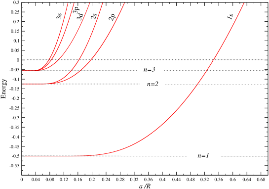
Figure 1: Spectrum of the Schrödinger hydrogen atom centered in a spherical cavity with the standard Dirichlet boundary condition (i.e. $\gamma=\infty$) as a function of $a/R$. The energies of states with quantum numbers $n=1,2,3$ are given in units of $Me^{4}$. The dotted lines represent the spectrum of the infinite system (cf. [23]).

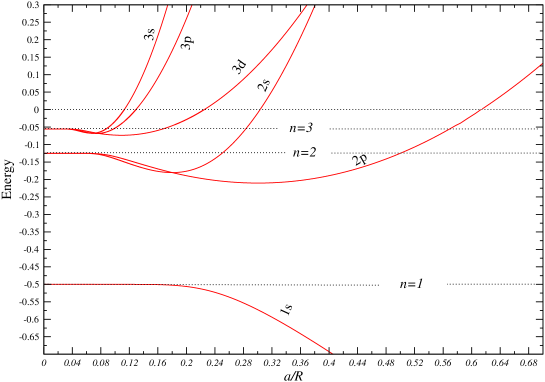
Figure 2: Spectrum of the Schrödinger hydrogen atom centered in a spherical cavity with Neumann boundary condition (i.e. $\gamma=0$) as a function of $a/R$. The energies of states with quantum numbers $n=1,2,3$ are given in units of $Me^{4}$. The dotted lines represent the spectrum of the infinite system (c.f. [23]).

As we discussed in Section 2.1, in the infinite volume the non-relativistic hydrogen atom enjoys an accidental $SO(4)$ symmetry generated by the angular momentum $\vec{L}$ together with the Runge-Lenz vector $\vec{R}$ of eq.(2.2), which results in an $n^{2}$-fold degeneracy of the bound state spectrum. The spectrum of hydrogen confined to a spherical cavity, on the other hand, no longer shows the accidental degeneracy. Since the boundary condition does not violate rotation invariance, $\vec{L}$ is still conserved, but $\vec{R}$ is not. This is because the application of the Runge-Lenz vector leads outside the domain of the Hamiltonian [23], as was already pointed out in [25, 27] for the Dirichlet boundary condition with $\gamma=\infty$. Relying on rotation invariance, we restrict ourselves to states $\Psi(\vec{r})=\psi_{nl}(r)Y_{ll}(\theta,\varphi)$ with the maximal $m=l$. On such states the raising operator $R_{+}=R_{x}+iR_{y}$ acts as [25]

$$R_{+}\Psi(\vec{r}) = \left[\frac{l+1}{M}\partial_{r}\psi_{nl}(r)+\left(e^{2}-\frac{l(l+1)}{Mr}\right)\psi_{nl}(r)\right]Y_{l+1,l+1}(\theta,\varphi)$$ (4.8)

$$= \chi_{n,l+1}(r)Y_{l+1,l+1}(\theta,\varphi).$$

After an application of $\vec{R}$ the wave function remains in the domain of the Hamiltonian only if the new wave function $\chi_{n,l+1}(r)$ also obeys the boundary condition

$$\gamma\chi_{n,l+1}(R)+\partial_{r}\chi_{n,l+1}(R)=0.$$ (4.9)

Inserting eq.(4.8) into this relation and using the boundary condition $\gamma\psi_{nl}(R)+\partial_{r}\psi_{nl}(R)=0$ as well as the radial Schrödinger equation (4.3) for $\psi_{nl}(r)$, one finds

$$\gamma\chi_{n,l+1}(R)+\partial_{r}\chi_{n,l+1}(R)=$$

$$\frac{l+1}{M}\left[-\gamma\left(\gamma-\frac{2}{R}\right)+\frac{l(l+2)}{R^{2}}-\frac{2Me^{2}}{R}-2ME\right]\psi_{nl}(R).$$ (4.10)

Since the right-hand side of eq.(4.1) does not vanish independent of the energy $E$, the new wave function $\chi_{n,l+1}(r)$ that results from the application of $R_{+}$ on $\psi_{nl}(r)$ does not obey the boundary condition eq.(4.9), and hence lies outside the domain of the Hamiltonian. Consequently, the Runge-Lenz vector $\vec{R}$ leads out of this domain, and thus no longer represents an accidental symmetry.

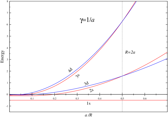
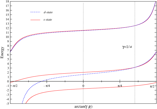
Figure 3: Top: Energy of s- and d-states for the Schrödinger hydrogen atom in a spherical cavity with $\gamma=1/a$ as a function of $a/R$. There is an accidental degeneracy for $R=2a$. Bottom: Energy of s- and d-states for a hydrogen atom in a spherical cavity with radius $R=2a$ as a function of $\arctan(\gamma R)$. The energies of the 3s and 4d states are very similar for all values of $\gamma$, but are identical only for $\gamma=2/R=1/a$ and for $\gamma=\pm\infty$. The energy is given in units of $Me^{4}$.

Interestingly, for $\gamma=\infty$ a remnant of the accidental symmetry persists even in a finite volume, however, only for the special cavity radius $R=(l+1)(l+2)a$ [25, 27]. Then a state with angular momentum $l$ is degenerate with a state of angular momentum $l+2$. In particular, for $R=2a$, the states 2s and 3d, 3s and 4d, 4s and 5d, etc. form multiplets of $1+5=6$ degenerate states, while for $R=6a$, the states 3p and 4f, 4p and 5f, 5p and 6f, etc. form multiplets of $3+7=10$ degenerate states. These accidental degeneracies are again due to the Runge-Lenz vector. They arise because, for the special values $R=(l+1)(l+2)a$, the operator $R_{+}^{2}$ maps $\psi_{nl}(r)$ back into the domain of the Hamiltonian. Indeed, one can show that $R_{+}^{2}\psi_{nl}(r)Y_{ll}(\theta,\varphi)=\chi_{n,l+2}(r)Y_{l+2,l+2}(\theta,\varphi)$ with

$$\chi_{n,l+2}(r) = \frac{2l+3}{M}\left(e^{2}-\frac{(l+1)(l+2)}{Mr}\right)\partial_{r}\psi_{nl}(r)$$

$$+ \left[\frac{(l+1)(l+2)}{M}\left(\frac{l(2l+3)}{Mr^{2}}-\frac{3e^{2}}{r}-2E\right)+e^{2}\left(e^{2}-\frac{l(l+1)}{Mr}\right)\right]\psi_{nl}(r).$$

(4.11)

Since for $\gamma=\infty$ the wave function obeys the Dirichlet boundary condition $\psi_{nl}(R)=0$, for

$$e^{2}-\frac{(l+1)(l+2)}{MR}=0\ \Rightarrow\ R=\frac{(l+1)(l+2)}{Me^{2}}=(l+1)(l+2)a,$$ (4.12)

the wave function $\chi_{n,l+2}(r)$ indeed obeys the same condition. Remarkably, the same accidental degeneracy arises for $R=(l+1)(l+2)a$ and $\gamma=2/R$ [26]. This follows from the fact that then $\gamma\psi_{nl}(R)+\partial_{r}\psi_{nl}(R)=0$ indeed implies $\gamma\chi_{n,l+2}(R)+\partial_{r}\chi_{n,l+2}(R)=0$. The remnant accidental degeneracies of the non-relativistic hydrogen atom in a spherical cavity are illustrated in figure 3.

4.2 The Relativistic Dirac Atom in a Spherical Cavity

Let us now consider the Dirac equation in a spherical cavity, i.e. we impose the boundary condition

$$\left(\begin{array}[]{c}\Psi_{3}(\vec{x})\\ \Psi_{4}(\vec{x})\end{array}\right)=\lambda(\vec{x})\left(\begin{array}[]{c}\Psi_{1}(\vec{x})\\ \Psi_{2}(\vec{x})\end{array}\right),\quad|\vec{x}|=R,$$ (4.13)

where $\vec{\sigma}\cdot\vec{e}_{r}\lambda(\vec{x})$ is an anti-Hermitean matrix. Again, we want to maintain the spherical symmetry, $[H,\vec{J}]=0$. We thus act with $J^{a}$ on a general Dirac spinor $\Psi(\vec{x})$ and demand that $\Psi(\vec{x})^{\prime}=J^{a}\Psi(\vec{x})$ still obeys the boundary condition

$$\lambda(\vec{x})\left(\begin{array}[]{c}\Psi_{1}(\vec{x})^{\prime}\\ \Psi_{2}(\vec{x})^{\prime}\end{array}\right) = \lambda(\vec{x})J^{a}\left(\begin{array}[]{c}\Psi_{1}(\vec{x})\\ \Psi_{2}(\vec{x})\end{array}\right)=\left(\begin{array}[]{c}\Psi_{3}(\vec{x})^{\prime}\\ \Psi_{4}(\vec{x})^{\prime}\end{array}\right)$$ (4.20)

$$= J^{a}\left(\begin{array}[]{c}\Psi_{3}(\vec{x})\\ \Psi_{4}(\vec{x})\end{array}\right)=J^{a}\lambda(\vec{x})\left(\begin{array}[]{c}\Psi_{1}(\vec{x})\\ \Psi_{2}(\vec{x})\end{array}\right).$$ (4.25)

This hence implies that $[J^{a},\lambda(\vec{x})]=0$. Similarly, the boundary condition should also maintain the parity symmetry $P$, such that $\Psi(\vec{x})^{\prime}=P\Psi(\vec{x})$ should again obey the boundary condition

$$\lambda(\vec{x})\left(\begin{array}[]{c}\Psi_{1}(\vec{x})^{\prime}\\ \Psi_{2}(\vec{x})^{\prime}\end{array}\right) = \lambda(\vec{x})\left(\begin{array}[]{c}\Psi_{1}(-\vec{x})\\ \Psi_{2}(-\vec{x})\end{array}\right)=\left(\begin{array}[]{c}\Psi_{3}(\vec{x})^{\prime}\\ \Psi_{4}(\vec{x})^{\prime}\end{array}\right)$$ (4.32)

$$= \left(\begin{array}[]{c}-\Psi_{3}(-\vec{x})\\ -\Psi_{4}(-\vec{x})\end{array}\right)=-\lambda(-\vec{x})\left(\begin{array}[]{c}\Psi_{1}(-\vec{x})\\ \Psi_{2}(-\vec{x})\end{array}\right).$$ (4.37)

This implies the restriction $\lambda(\vec{x})=-\lambda(-\vec{x})$. Rotation invariance and parity limit the anti-Hermitean matrix that characterizes the boundary condition to

$$\lambda(\vec{x})=i\nu\vec{\sigma}\cdot\vec{e}_{r},$$ (4.38)

such that $\vec{\sigma}\cdot\vec{e}_{r}\lambda(\vec{x})=i\nu{\mathbbm{1}}$ is indeed anti-Hermitean. Let us further investigate whether $K$ remains a symmetry in the finite volume. For this purpose we act with $K$ on the Dirac spinor $\Psi(\vec{x})$, and we ask once more whether the new spinor $\Psi(\vec{x})^{\prime}=K\Psi(\vec{x})$ still obeys the boundary condition. This is the case only if

$$\lambda(\vec{x})\left(\begin{array}[]{c}\Psi_{1}(\vec{x})^{\prime}\\ \Psi_{2}(\vec{x})^{\prime}\end{array}\right) = \lambda(\vec{x})(\vec{\sigma}\cdot\vec{L}+{\mathbbm{1}})\left(\begin{array}[]{c}\Psi_{1}(\vec{x})\\ \Psi_{2}(\vec{x})\end{array}\right)=\left(\begin{array}[]{c}\Psi_{3}(\vec{x})^{\prime}\\ \Psi_{4}(\vec{x})^{\prime}\end{array}\right)$$ (4.45)

$$= -(\vec{\sigma}\cdot\vec{L}+{\mathbbm{1}})\lambda(\vec{x})\left(\begin{array}[]{c}\Psi_{1}(\vec{x})\\ \Psi_{2}(\vec{x})\end{array}\right),$$ (4.48)

which is indeed satisfied since

$$\{\lambda(\vec{x}),\vec{\sigma}\cdot\vec{L}+{\mathbbm{1}}\}=\{i\nu\vec{\sigma}\cdot\vec{e}_{r},\vec{\sigma}\cdot\vec{L}+{\mathbbm{1}}\}=0.$$ (4.49)

Next, we want to investigate whether the Johnson-Lippmann operator also leaves the boundary condition invariant. Hence, we now ask whether $\Psi(\vec{x})^{\prime}=A\Psi(\vec{x})$ also obeys the boundary condition, which is the case only if

$$\lambda(\vec{x})\left(\begin{array}[]{c}\Psi_{1}(\vec{x})^{\prime}\\ \Psi_{2}(\vec{x})^{\prime}\end{array}\right) = \left[\lambda(\vec{x})\frac{i}{Mc}(\vec{\sigma}\cdot\vec{L}+{\mathbbm{1}})\vec{\sigma}\cdot\vec{p}-\lambda(\vec{x})\alpha\vec{\sigma}\cdot\vec{e}_{r}\right.$$ (4.52)

$$- \left.\lambda(\vec{x})\frac{i\alpha}{McR}(\vec{\sigma}\cdot\vec{L}+{\mathbbm{1}})\lambda(\vec{x})\right]\left(\begin{array}[]{c}\Psi_{1}(\vec{x})\\ \Psi_{2}(\vec{x})\end{array}\right)$$ (4.55)

$$= \left(\begin{array}[]{c}\Psi_{3}(\vec{x})^{\prime}\\ \Psi_{4}(\vec{x})^{\prime}\end{array}\right)=\left[\frac{i\alpha}{McR}(\vec{\sigma}\cdot\vec{L}+{\mathbbm{1}})\right.$$ (4.58)

$$- \left.\frac{i}{Mc}(\vec{\sigma}\cdot\vec{L}+{\mathbbm{1}})\vec{\sigma}\cdot\vec{p}\lambda(\vec{x})-\alpha\vec{\sigma}\cdot\vec{e}_{r}\lambda(\vec{x})\right]\left(\begin{array}[]{c}\Psi_{1}(\vec{x})\\ \Psi_{2}(\vec{x})\end{array}\right).$$ (4.61)

(4.62)

Using $[\lambda(\vec{x}),\vec{\sigma}\cdot\vec{e}_{r}]=0$, this condition would indeed be satisfied if the following identity holds

$$\{\lambda(\vec{x}),(\vec{\sigma}\cdot\vec{L}+{\mathbbm{1}})\vec{\sigma}\cdot\vec{p}\}=\frac{\alpha}{R}\left(\lambda(\vec{x})(\vec{\sigma}\cdot\vec{L}+{\mathbbm{1}})\lambda(\vec{x})+\vec{\sigma}\cdot\vec{L}+{\mathbbm{1}}\right)\ \Rightarrow$$

$$i\nu\{\vec{\sigma}\cdot\vec{e}_{r},(\vec{\sigma}\cdot\vec{L}+{\mathbbm{1}})\vec{\sigma}\cdot\vec{p}\}=\frac{\alpha}{R}(\nu^{2}+1)(\vec{\sigma}\cdot\vec{L}+{\mathbbm{1}}).$$ (4.63)

It is straightforward to show that

$$i\{\vec{\sigma}\cdot\vec{e}_{r},(\vec{\sigma}\cdot\vec{L}+{\mathbbm{1}})\vec{\sigma}\cdot\vec{p}\}=(\vec{\sigma}\cdot\vec{L}+{\mathbbm{1}})i[\vec{\sigma}\cdot\vec{p},\vec{\sigma}\cdot\vec{e}_{r}]=\frac{2}{R}(\vec{\sigma}\cdot\vec{L}+{\mathbbm{1}})^{2},$$ (4.64)

which implies that $A$ maintains the boundary condition if

$$\alpha\frac{\nu^{2}+1}{2\nu}=\vec{\sigma}\cdot\vec{L}+{\mathbbm{1}}=k=\pm\left(j+\frac{1}{2}\right).$$ (4.65)

Obviously, this relation cannot hold as an operator identity. Still, it can be satisfied for states with an appropriate $k$-value and for specific values of $\nu$. One might then conclude that, like in the non-relativistic case, a remnant accidental degeneracy arises for particular states and for specific values of the self-adjoint extension parameter. However, the situation is more subtle. In particular, since $\{K,A\}=0$, an application of $A$ changes the sign of $k$. This means that, for a fixed value of $\nu$, eq.(4.65) is no longer satisfied for $-k$, and thus another application of $A$ will inevitably lead out of the domain of $H$. Since repeated applications of $H$ or $K$, on the other hand, leave the wave function inside the domain, eq.(2.16), which relates $A^{2}$ to $H^{2}$ and $K^{2}$ in the infinite volume, is no longer satisfied in a finite volume. In fact, $H$ and $A$ no longer commute as operators restricted to the domain of $H$. This implies that $A$ no longer generates an accidental symmetry, and the corresponding degeneracy is lifted in a finite volume.

Let us now investigate the spectrum of relativistic hydrogen in a spherical cavity in more detail. First we make a separation ansatz for the wave function

$$\Psi(\vec{x})=\left(\begin{array}[]{c}\Psi_{1}(\vec{x})\\ \Psi_{2}(\vec{x})\\ \Psi_{3}(\vec{x})\\ \Psi_{4}(\vec{x})\end{array}\right)=\left(\begin{array}[]{c}\psi_{A}(r){\cal Y}_{jj_{3}l_{A}}(\theta,\varphi)\\ i\psi_{B}(r){\cal Y}_{jj_{3}l_{B}}(\theta,\varphi)\end{array}\right).$$ (4.66)

For $k=j+\frac{1}{2}$ we have $l_{A}=j-\frac{1}{2}$ and $l_{B}=j+\frac{1}{2}$, while for $k=-(j+\frac{1}{2})$, $l_{A}=j+\frac{1}{2}$ and $l_{B}=j-\frac{1}{2}$. For $j=l+\frac{1}{2}$ the spin-angular functions are given by

$${\cal Y}_{jj_{3}l}(\theta,\varphi)=\sqrt{\frac{l+j_{3}+\frac{1}{2}}{2l+1}}Y_{l,j_{3}-\frac{1}{2}}(\theta,\varphi)\left(\begin{array}[]{c}1\\ 0\end{array}\right)+\sqrt{\frac{l-j_{3}+\frac{1}{2}}{2l+1}}Y_{l,j_{3}+\frac{1}{2}}(\theta,\varphi)\left(\begin{array}[]{c}0\\ 1\end{array}\right),$$ (4.67)

while for $j=l-\frac{1}{2}$

$${\cal Y}_{jj_{3}l}(\theta,\varphi)=-\sqrt{\frac{l-j_{3}+\frac{1}{2}}{2l+1}}Y_{l,j_{3}-\frac{1}{2}}(\theta,\varphi)\left(\begin{array}[]{c}1\\ 0\end{array}\right)+\sqrt{\frac{l+j_{3}+\frac{1}{2}}{2l+1}}Y_{l,j_{3}+\frac{1}{2}}(\theta,\varphi)\left(\begin{array}[]{c}0\\ 1\end{array}\right).$$ (4.68)

Here $Y_{lm}(\theta,\varphi)$ are the usual spherical harmonics. The radial equations then take the form

$$\left(Mc^{2}-\frac{e^{2}}{r}\right)\psi_{A}(r)-c\left(\partial_{r}+\frac{1+k}{r}\right)\psi_{B}(r)=E\psi_{A}(r),$$

$$\left(-Mc^{2}-\frac{e^{2}}{r}\right)\psi_{B}(r)+c\left(\partial_{r}+\frac{1-k}{r}\right)\psi_{A}(r)=E\psi_{B}(r).$$ (4.69)

The cavity boundary condition is given by

$$i\nu\vec{e}_{r}\cdot\vec{\sigma}\psi_{A}(R){\cal Y}_{jj_{3}l_{A}}(\theta,\varphi)=-i\nu\psi_{A}(R){\cal Y}_{jj_{3}l_{B}}(\theta,\varphi)=i\psi_{B}(R){\cal Y}_{jj_{3}l_{B}}(\theta,\varphi)\ \Rightarrow$$

$$\nu\psi_{A}(R)=-\psi_{B}(R).$$ (4.70)

The resulting finite volume spectra for $\nu=\infty$ (i.e. Dirichlet boundary conditions) and for $\nu=0$ (i.e. Neumann boundary conditions) are illustrated in Figs. 4 and 5, respectively. In order to make the effects easily visible we have chosen very large unphysical values of $\alpha$.

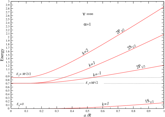
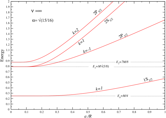
Figure 4: Spectrum of the Dirac hydrogen atom centered in a spherical cavity with the standard Dirichlet boundary condition (i.e. $\nu=\infty$) for $\alpha=1$ (top) and for $\alpha=\sqrt{15/16}$ (bottom), as a function of $a/R$. The energies of states with quantum numbers $n=1$ and 2 are given in units of $M$. The dotted lines represent the spectrum of the infinite system.

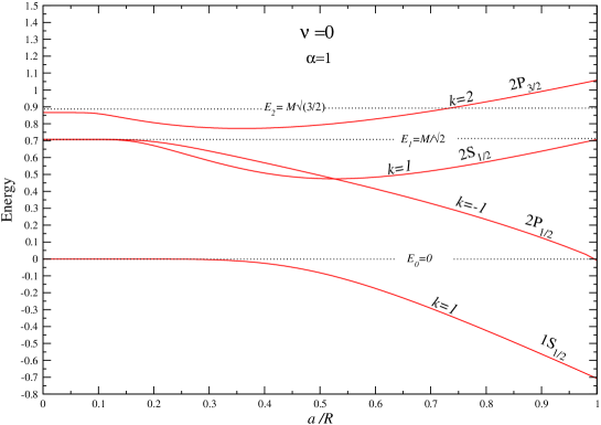
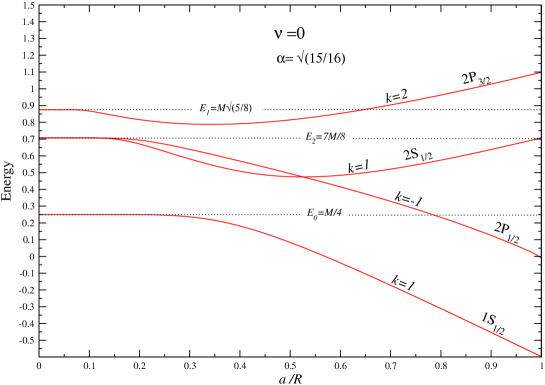
Figure 5: Spectrum of the Dirac hydrogen atom centered in a spherical cavity with Neumann boundary condition (i.e. $\nu=0$) for $\alpha=1$ (top) and for $\alpha=\sqrt{15/16}$ (bottom), as a function of $a/R$. The energies of states with quantum numbers $n=1$ and 2 are given in units of $M$. The dotted lines represent the spectrum of the infinite system.

In both cases, we see that the states 2S_1/2 and 2P_1/2, which are accidentally degenerate in the infinite volume, are split in the finite cavity. With Dirichlet boundary conditions ($\nu=\infty$) the energies increase with decreasing cavity radius, while for Neumann boundary conditions ($\nu=0$) the energy of some states decreases.

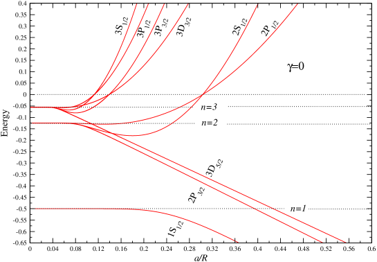
Figure 6: Spectrum of the Pauli hydrogen atom centered in a spherical cavity with Neumann boundary condition (i.e. $\gamma=0$) as a function of $a/R$. The energies of states with quantum numbers $n=1,2,3$ are given in units of $Me^{4}$. The dotted lines represent the spectrum of the infinite system.

4.3 The Non-relativistic Pauli Atom in a Spherical Cavity

Finally, we proceed to the non-relativistic limit of the Dirac equation, which leads us to the Pauli equation

$$H=Mc^{2}+\frac{\left(\vec{p}c+e\vec{A}(\vec{x})\right)^{2}}{2Mc^{2}}-e\Phi(\vec{x})+\mu\vec{\sigma}\cdot\vec{B}(\vec{x}).$$ (4.71)

Since we have no external magnetic field, at least to the leading order we are working at, spin decouples and the Pauli equation reduces to two copies of the Schrödinger equation. In particular, we have neglected the sub-leading spin-orbit couplings in the Hamiltonian. Still, as we discussed in Subsection 3.3, the spin explicitly enters the boundary condition

$$\gamma(\vec{x})\Psi(\vec{x})+\vec{n}(\vec{x})\cdot\left[\vec{\nabla}\Psi(\vec{x})-i\vec{\sigma}\times\vec{\nabla}\Psi(\vec{x})\right]=0,$$ (4.72)

which thus leads to a spin-orbit coupling induced by the cavity wall. The Hermitean matrix $\gamma(\vec{x})$, which results from the anti-Hermitean matrix $\lambda(\vec{x})$ in the non-relativistic limit, is given by

$$\gamma(\vec{x})=-2Mci\vec{n}(\vec{x})\cdot\vec{\sigma}\lambda(\vec{x})=2Mc\nu{\mathbbm{1}}.$$ (4.73)

For $j=l+\frac{1}{2}$ the boundary condition of eq.(4.72) reduces to

$$\gamma\psi_{nl}(R)+\partial_{r}\psi_{nl}(R)-\frac{l}{R}\psi_{nl}(R)=0,$$ (4.74)

while for $j=l-\frac{1}{2}$

$$\gamma\psi_{nl}(R)+\partial_{r}\psi_{nl}(R)+\frac{l+1}{R}\psi_{nl}(R)=0,$$ (4.75)

The spectrum of the Pauli equation for Neumann boundary conditions (i.e. $\gamma=0$) is illustrated in Fig. 6. It differs from the spectrum of Fig. 2 because now the angular momentum enters the boundary condition.

Let us now address the question of remnant accidental degeneracies that persist even in a finite volume. As we discussed in Subsection 4.1, for the Schrödinger atom these exist for $R=(l+1)(l+2)a$ and $\gamma=2/R$ or $\infty$, because, in these cases, two applications of the Runge-Lenz vector lead back into the domain of the Hamiltonian. For the Dirac atom in a finite volume, on the other hand, repeated applications of the Johnson-Lippmann operator do not lead back into the domain of the Hamiltonian, and thus the accidental degeneracy is lifted in a finite volume (c.f. Subsection 4.2).

As we will see now, just as for the Schrödinger atom, for the Pauli atom some accidental degeneracies persist in a finite cavity. We start again from eq.(4.1), take its derivative with respect to $r$, and then eliminate $\partial_{r}^{2}\psi_{nl}(r)$ by using the radial Schrödinger equation (4.3). We then impose the boundary condition eq.(4.74) when $j=l+\frac{1}{2}$, or eq.(4.75) when $j=l-\frac{1}{2}$. Finally, we ask under what circumstances the wave function $\chi_{n,l+2}(r)$ of eq.(4.1) satisfies the corresponding boundary condition

$$\gamma\chi_{n,l+2}(R)+\partial_{r}\chi_{n,l+2}(R)-\frac{l+2}{R}\chi_{n,l+2}(R)=0,$$ (4.76)

when $j^{\prime}=l+2+\frac{1}{2}=l+\frac{5}{2}$, or

$$\gamma\chi_{n,l+2}(R)+\partial_{r}\chi_{n,l+2}(R)+\frac{l+3}{R}\chi_{n,l+2}(R)=0,$$ (4.77)

when $j^{\prime}=l+2-\frac{1}{2}=l+\frac{3}{2}$, for all values of the energy $E$. For $j=l+\frac{1}{2}$ and $j^{\prime}=l+\frac{5}{2}$ this turns out to be the case for

$$R=\frac{(l+1)(l+2)(2l+5)a}{2l+3},\quad\gamma=-\frac{1}{2(l+1)(l+2)a},\ \mbox{or}\ \gamma=\frac{1}{(l+1)a}.$$ (4.78)

For $j=l+\frac{1}{2}$ and $j^{\prime}=l+\frac{3}{2}$, on the other hand, the conditions can be satisfied only when $e^{2}=0$ and $\gamma=0$. For $j=l-\frac{1}{2}$ and $j^{\prime}=l+\frac{5}{2}$ one obtains

$$R=2(l+1)(l+2)a,\quad\gamma=-\frac{1}{2(l+1)(l+2)a}=-\frac{1}{R},\ \mbox{or}\ \gamma=\frac{3}{2(l+1)(l+2)a}=\frac{3}{R},$$ (4.79)

and, finally, for $j=l-\frac{1}{2}$ and $j^{\prime}=l+\frac{3}{2}$ one finds

$$R=\frac{(l+1)(l+2)(2l+1)a}{2l+3},\quad\gamma=-\frac{1}{2(l+1)(l+2)a},\ \mbox{or}\ \gamma=-\frac{1}{(l+2)a}.$$ (4.80)

The remnant accidental symmetries for the Pauli hydrogen atom are illustrated in Fig. 7.

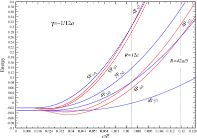
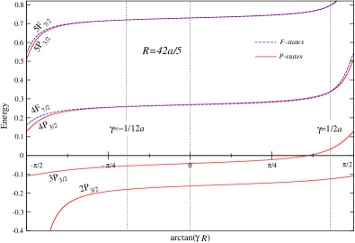
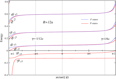
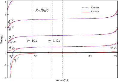
Figure 7: Top left: Energy of P- and F-states with $n=4$ and 5 for the Pauli hydrogen atom in a spherical cavity with $\gamma=-\frac{1}{12a}$ as a function of $a/R$. There are accidental degeneracies (indicated by the vertical dashed lines) of the 4P_3/2 with the 4F_7/2 for $R=\frac{42}{5}a$, as well as of the 4P_1/2 with the 4F_7/2 and of the 5P_1/2 with the 5F_7/2 states for $R=12a$. Top right and bottom: Energy of P- and F-states for the Pauli hydrogen atom in a spherical cavity as a function of $\arctan(\gamma R)$ at fixed cavity radius: $R=\frac{42}{5}a$ (top right), $R=12a$ (bottom left), and $R=\frac{18}{5}a$ (bottom right): The energies of the high-lying P- and F-states are very similar for all values of $\gamma$, but are identical only for the special values indicated by the vertical dashed lines. The energy is given in units of $Me^{4}$.

5 Conclusions

We have investigated the accidental symmetry in the relativistic hydrogen atom confined to a spherical cavity with perfectly reflecting boundary conditions. In the infinite volume the Johnson-Lippman operator $A$, which is the relativistic analog of the Runge-Lenz vector $\vec{R}$, commutes with the Hamiltonian, thus leading to accidental degeneracies in the energy spectrum. When the system is placed in a finite volume, the accidental symmetry is lifted. This is because a repeated application of the Johnson-Lippman operator leads out of the domain of the Hamiltonian. In the non-relativistic case, for specific values of the cavity radius $R$ and the self-adjoint extension parameter $\gamma$, a repeated application of $\vec{R}$ leads back into the domain of the Hamiltonian, and thus some accidental degeneracy persists even in a finite volume. Because repeated applications of $A$ do not lead back into the domain of the Hamiltonian, this is not the case for the Dirac equation. Interestingly, in the Pauli equation with spin, which results as the non-relativistic limit of the Dirac equation, the boundary conditions induce non-trivial spin-orbit couplings. Remarkably, in this case, for specific values of the cavity radius $R$ and the self-adjoint extension parameter $\gamma$, a repeated application of $\vec{R}$ again leads back into the domain of the Hamiltonian, and thus some accidental degeneracy persists in a finite volume.

Our investigation shows that the subtle issues of Hermiticity versus self-adjointness and the domain structure of quantum mechanical Hamiltonians hold the key to understanding in detail what happens to a hydrogen atom when it is confined in a spherical cavity. The same is true for other accidental symmetries, for example, for the Landau level problem [8], for a particle on a cone [23], or for the harmonic oscillator [23, 24]. This underscores that the theory of self-adjoint extensions is not just a mathematical curiosity, but of great importance for understanding the physics of confined systems.

References

- [1] J. Bertrand, C. R. Acad. Sci. Paris 77 (1873) 849.
- [2] H. V. McIntosh, in Group Theory and its Applications, Vol. 2 (1971) 75, Academic Press, Inc. New York and London.
- [3] V. Fock, Z. Physik 98 (1935) 145.
- [4] V. Bargmann, Z. Physik 99 (1936) 576.
- [5] W. Lenz, Z. Physik 24 (1924) 197.
- [6] L. D. Landau, Z. Physik 64 (1930) 629.
- [7] M. H. Johnson and B. A. Lippmann, Phys. Rev. 76 (1949) 828.
- [8] M. H. Al-Hashimi and U.-J. Wiese, Ann. Phys. 324 (2009) 343.
- [9] M. H. Al-Hashimi and U.-J. Wiese, Ann. Phys. 323 (2008) 92.
- [10] J. von Neumann, Mathematische Grundlagen der Quantenmechanik, Berlin, Springer (1932).
- [11] M. Reed and B. Simon, Methods of Modern Mathematical Physics II, Fourier Analysis, Self-Adjointness, Academic Press Inc., New York (1975).
- [12] R. Balian and C. Bloch, Ann. Phys. 60 (1970) 401.
- [13] M. Carreau and E. Farhi, Phys. Rev. D42 (1990) 1194.
- [14] G. Bonneau, J. Faraut, and G. Valent, Am. J. Phys. 69 (2001) 322.
- [15] M. H. Al-Hashimi and U.-J. Wiese, Ann. Phys. 327 (2012) 2742.
- [16] M. H. Al-Hashimi, M. Salman, A. Shalaby, and U.-J. Wiese, Ann. Phys. 337 (2013) 1.
- [17] A. Michels, J. de Boer, and A. Bijl, Physica 4 (1937) 981.
- [18] A. Sommerfeld and H. Welker, Ann. Phys. 424 (1938) 56.
- [19] S. R. de Groot and C. A. ten Seldam, Physica 12 (1946) 669.
- [20] E. P. Wigner, Phys. Rev. 94 (1954) 77.
- [21] P. W. Fowler, Mol. Phys. 53 (1984) 865.
- [22] P. O. Frömann, S. Yngve, and N. Frömann, J. Math. Phys. 28 (1987) 1813.
- [23] M. H. Al-Hashimi and U.-J. Wiese, Ann. Phys. 327 (2012) 1.
- [24] M. H. Al-Hashimi, Molecular Physics 111 (2013) 225.
- [25] V. I. Pupyshev and A. V. Scherbinin, Chem. Phys. Lett. 295 (1998) 217.
- [26] A. V. Scherbinin and V. I. Pupyshev, Russ. J. Phys. Chem. 74 (2000) 292.
- [27] V. I. Pupyshev and A. V. Scherbinin, Phys. Lett. A 299 (2002) 371.
- [28] W. Gordon, Z. Phys. 48 (1928) 11.
- [29] C. G. Darwin, Proc. R. Soc. London A118 (1928) 654.
- [30] F. D. Pidduck, J. London Math. Soc. 4 (1929) 163.
- [31] L. C. Biedenharn, Phys. Rev. 126 (1962) 845.
- [32] M. K. F. Wong and H.-Y. Yeh, Phys. Rev. D25 (1982) 3396.
- [33] J. M. Cohen and B. Kuharetz, J. Math. Phys. 34 (1993) 4964.
- [34] V. M. Villalba, Rev. Mex. Phys. 42 (1996) 1.
- [35] M. H. Johnson and B. A. Lippmann, Phys. Rev. 78 (1950) 329(A).
- [36] L. C. Biedenharn, Found. Phys. 13 (1983) 13.
- [37] C. V. Sukumar, J. Phys. A18 (1985) L697.
- [38] P. D. Jarvis and G. E. Stedman, J. Phys. A19 (1986) 1373.
- [39] J. P. Dahl and T. Jorgensen, Int. J. Quant. Chem. 53 (1995) 161.
- [40] A. Kirchberg, J. D. Lange, P. A. G. Pisani, and A. Wipf, Ann. Phys. 303 (2003) 359.
- [41] P. Alberto, C. Fiolhais, V. M. S. Gil, Eur. J. Phys. 17 (1996) 19.
- [42] P. Alberto, S. Das, E. C. Vagenas, Phys. Lett. A375 (2011) 1436.
- [43] V. Alonso and S. De Vincenzo, J. Phys. A: Math. Gen. 30 (1997) 8573.
- [44] A. Chodos, R. L. Jaffe, K. Johnson, C. B. Thorn, and V. F. Weisskopf, Phys. Rev. D9 (1974) 3471.
- [45] A. Chodos, R. L. Jaffe, K. Johnson, and C. B. Thorn, Phys. Rev. D10 (1974) 2599.
- [46] P. Hasenfratz and J. Kuti, Phys. Rept. 40 (1978) 75.