Quantum single-particle properties in a one-dimensional curved space

Abstract

We consider one particle confined to a deformed one-dimensional wire. The quantum mechanical equivalent of the classical problem is not uniquely defined. We describe several possible hamiltonians and corresponding solutions for a finite wire with fixed endpoints and non-vanishing curvature. We compute and compare the disparate eigenvalues and eigenfunctions obtained from different quantization prescriptions. The JWKB approximation without potential leads precisely to the square well spectrum and the coordinate dependent stretched or compressed box related eigenfunctions. The geometric potential arising from an adiabatic expansion in terms of curvature is at best only valid for very small curvature.

I Introduction

Advances in optical trapping techniques makes it possible to trap cold atoms in what is effectively 1 or 2 dimensionalricardez2010 ; reitz2012 ; arnold2012 ; macdonald2002 ; bhatta2007 ; sague2008 ; pang2005 . An interesting direction of this is the ability to create effective quantum wires of varying shape and curvature. An advantage of these lower dimensional setups are the how they can be shaped in ways that provide stabillity against short range collapse of polar molecules. Another thing is how long range interactions can shortcut through the second or third dimensions, and create novel interactions in 1 and 2 dimension law2008 ; huhta2010 ; schmelcher2011 ; zampetaki2013 ; pedersen2014 .

When describing the motion of an atom moving along such a wire there are at least two different approaches. The first is to solve the problem fully in three dimensions, and treat the trapping potential as any other potential. This approach is difficult to solve both analytically and numerically, unless the trapping potential is highly symmetric. The other approach is to develop a quantum mechanical description of the system in one dimension. How to do this is not well defined for general structures. This paper will discuss various quantization prescriptions of the classical motion, both in general and in particular focussed on the one-dimensional wire problem.

In general, position dependent masses present problems in quantizing classical motion. This problem was already recognized by Schrödinger sch26 , and in the dynamical evolution of nuclear shapes from equilibrium through saddle points to separated fission fragments hof71 . The problem appears first of all when the starting points are generalized masses obtained independent from potential energies as for example through classical cranking type of models pau74 and micro-macro energy calculations bra72

The motion can be constrained geometrically by an external field and it is then possible to simulate this physical situation by steep confining walls in forbidden directions. Then the procedure can be more straightforward by approximately solving the full many-dimensional problem. The effects of the repulsive walls may then be approximated by applying an adiabatic expansion which results in a potential reflecting the geometric properties of the confinement PhysRevA.89.033630 . We shall compare results from different quantization prescriptions.

The purpose of the present paper is to exhibit similarities and differences between quantum mechanical results arising from different quantizations of a single-particle hamiltonian in one dimension. In general we shall allow an undetermined coordinate dependent parametrization of the particle mass. In section II we develop a classical description of a particle confined to move in along a curved wire. In section III we show the different choices of how to quantize the system. In the sections IV and V we look at three different choices of wire, and using the different approaches from section III, we calculate the spectra and the eigenfunctions. Finally in section VI we give a summary of the discussions and an outlook.

II Classical Description

We consider one particle confined to move in a one-dimensional trap. The particle is assumed to be point like with no internal structure and have a mass of $m_{0}$. The trapping geometry is going to be several different deformations of a helix. This one dimensional curve is defined by a parametrization $F:\operatorname{\mathbb{R}}\rightarrow\operatorname{\mathbb{R}}^{3}$. The parameterizations discussed in this paper will all be of the form

$$\left\{x,y,z\right\}=R\cdot\left\{f_{x}(\phi)\cos{\phi},f_{y}(\phi)\sin{\phi},f_{z}(\phi)\right\}.$$ (1)

Instead of using the full three dimensional set of coordinates we use $\phi$, to describe the position of the particle along the curve.

The classical velocity is then $(\dot{x},\dot{y},\dot{z})$, where the dots denote time derivation. The corresponding classical kinetic energy, $T$, of the particle in three dimensions is then given by

$$T=\frac{1}{2}m_{0}\left(\dot{x}^{2}+\dot{y}^{2}+\dot{z}^{2}\right).$$ (2)

Then $T$ can be transformed through Eq. (1) to only depend on the angular position, $\phi$, and velocity, $\dot{\phi}$, along the curve, that is

$$T(\phi,\dot{\phi})=\frac{1}{2}m_{0}(x^{\prime 2}+y^{\prime 2}+z^{\prime 2})\dot{\phi}^{2}\equiv\frac{1}{2}m(\phi)\dot{\phi}^{2}\;,$$ (3)

which defines the effective mass $m(\phi)$. For the parametrization in Eq. (1) this yields the explicit expression

$$\begin{split}m(\phi)=m_{0}R^{2}&\left[(f^{\prime 2}_{x}+f^{2}_{y})\cos^{2}{\phi}+(f^{2}_{x}+f^{\prime 2}_{y})\sin^{2}{\phi}\right.\\ &\left.+(f_{x}f^{\prime}_{x}-f_{y}f^{\prime}_{y})\sin(2\phi)+f^{\prime 2}_{z}\right]\;,\end{split}$$ (4)

where the primes denote derivatives with respect to $\phi$.

A useful quantity is the canonical conjugate momentum, $p_{\phi}$, to the position $\phi$ along the curve, that is taylor2005classical

$$p_{\phi}=\frac{\partial T}{\partial\dot{\phi}}=m(\phi)\dot{\phi}\;,$$ (5)

which provides the kinetic energy in canonical form

$$T=\frac{p_{\phi}^{2}}{2m(\phi)}\;.$$ (6)

The coordinate dependent mass in Eq. (4) is a key quantity. The present parametrization in Eq. (1) only provides $\phi$-independent effective mass when the functions $f^{\prime}_{z}$ and $f_{x}=f_{y}$ are independent of $\phi$. These are both necessary and sufficient conditions for the constant effective mass, $m(\phi)=m_{0}R^{2}(f_{x}^{2}+f^{\prime 2}_{z})$, of a regular helix.

Another simple case is $f_{x}=f_{y}$ where we have

$$m(\phi)=m_{0}R^{2}(f_{x}^{2}+f^{\prime 2}_{x}+f^{\prime 2}_{z}),$$ (7)

which still may contain a $\phi$-dependence. When both $f_{x}$ and $f_{y}$ are constants, which corresponds to the parametrization of an ellipse in the x-y plane, we have

$$m(\phi)=m_{0}R^{2}\left(f_{x}^{2}\cos^{2}{\phi}+f_{y}^{2}\sin^{2}{\phi}+f^{\prime 2}_{z}\right).$$ (8)

If furthermore, $f_{x}=f_{y}$ and $f^{\prime}_{z}=0$ the helix reduces to a circle in the $x-y$ plane, and the mass becomes $m_{0}R^{2}$, which is just the initial mass scaled by the $R^{2}$-factor that appears when using the dimensionless $\phi$-coordinate. We conclude that the effects of a non-constant effective mass require more than the regular helix, and we need to consider angle-dependent $f$-functions.

III Quantizing the motion

In this section we shall consider different prescriptions to quantize the particle motion on the curves parameterized through the classical physics described in the previous section.

III.1 Quantizing in one dimension

Without an external potential on the particle the hamiltonian only contains terms arising from the kinetic energy in Eq. (6). The complication may be the position dependent effective mass. The straightforward quantization is from Eq. (6) with $p_{\phi}=-i\hbar\frac{\partial}{\partial\phi}$, but ordering of this operator and the mass term, $1/m(\phi)$, is now important. We demand that the hamiltonian is hermitian and the eigenenergies of the system must consequently be real.

A general structure of the kinetic energy operator is

$$-\frac{\hbar^{2}}{2}\frac{1}{m^{a}}\frac{\partial}{\partial\phi}\frac{1}{m^{b}}\frac{\partial}{\partial\phi}\frac{1}{m^{c}}\;,$$ (9)

where $a+b+c=1$ and hermiticity requires $a=c$. An even more general form would be to allow $a\neq c$, but instead symmetrizing afterwards, that is

$$-\frac{\hbar^{2}}{4}\bigg{(}\frac{1}{m^{a}}\frac{\partial}{\partial\phi}\frac{1}{m^{b}}\frac{\partial}{\partial\phi}\frac{1}{m^{c}}+\frac{1}{m^{c}}\frac{\partial}{\partial\phi}\frac{1}{m^{b}}\frac{\partial}{\partial\phi}\frac{1}{m^{a}}\bigg{)}\;.$$ (10)

The quantization in Eq. (10) is problematic for discontinuous potentials, which breaks the hermitian property dek99 . This does not apply to our case and we shall not a priori reject the two different terms in Eq. (10). To be specific we choose typical examples with properties from Eqs. (9) and (10), that is $a=c=0,b=1$ and $b=c=0,a=1$, respectively.

The first of these choices of an effective mass hamiltonian is with the mass placed between the two momentum operators, that is

$$H_{1}=-\frac{\hbar^{2}}{2}\frac{\partial}{\partial\phi}\frac{1}{m(\phi)}\frac{\partial}{\partial\phi}\;.$$ (11)

By taking the first order derivative of the effective mass the hamiltonian can be rewritten as

$$H_{1}=-\frac{\hbar^{2}}{2m(\phi)}\frac{\partial^{2}}{\partial\phi^{2}}+\frac{\hbar^{2}m^{\prime}(\phi)}{2m^{2}(\phi)}\frac{\partial}{\partial\phi}.$$ (12)

We note here that the position dependent effective mass, results in an extra term in the hamiltonian. Not only does this hamiltonian contain a first order derivative of the effective mass, but this term also contains a first order derivative. Both features are not present in a normal hamiltonian only containing a kinetic energy part with a constant mass.

The first order derivative can be removed as usual by the substitution of the total wavefunction, $\Psi=m^{1/2}\psi$, into the Schrödinger equation, $(H_{1}-E)\Psi=0$. The corresponding new hamiltonian acting on the reduced wavefunction, $\psi$ then becomes

$${H}_{EM_{1}}=-\frac{\hbar^{2}}{2m(\phi)}\frac{\partial^{2}}{\partial\phi^{2}}-\frac{\hbar^{2}}{4m^{2}(\phi)}\bigg{(}m^{\prime\prime}(\phi)-\frac{3m^{\prime 2}(\phi)}{2m(\phi)}\bigg{)}\;,$$ (13)

where the energy remains unchanged while a centrifugal barrier term appears, and the Schrödinger equation becomes $(H_{EM_{1}}-E)\psi=0$.

Another possible choice of hamiltonian is one explicitly constructed as hermitian with two terms. One term with the effective mass before the momentum operators, and another term with the effective mass after the momentum operators, that is

$$H_{2}=-\frac{\hbar^{2}}{4}\left(\frac{\partial^{2}}{\partial\phi^{2}}\frac{1}{m(\phi)}+\frac{1}{m(\phi)}\frac{\partial^{2}}{\partial\phi^{2}}\right)\;.$$ (14)

Calculating the derivatives of $m(\phi)$ we end up with a hamiltonian, with the same first order derivative term appearing in $H_{1}$, and in addition another effective potential. In total we get

$$H_{2}=-\frac{\hbar^{2}}{2m(\phi)}\frac{\partial^{2}}{\partial\phi^{2}}+\frac{\hbar^{2}m^{\prime}(\phi)}{2m^{2}(\phi)}\frac{\partial}{\partial\phi}-\frac{\hbar^{2}}{4}\frac{\partial^{2}}{\partial\phi^{2}}\left(\frac{1}{m(\phi)}\right).$$ (15)

The extra potential term is the only difference between $H_{1}$ and $H_{2}$. It contains terms of up to second order in the derivative of the mass. The first order angular derivative is removed as in $H_{1}$ resulting in the hamiltonian, $H_{EM_{2}}$, acting on the reduced wavefunction, $\psi$. The difference between these two hamiltonians amounts to an additional potential, that is

$$V_{EM_{2}} = H_{EM_{1}}-H_{EM_{2}}$$

$$= \frac{\hbar^{2}}{4}\frac{\partial^{2}}{\partial\phi^{2}}\left(\frac{1}{m(\phi)}\right)=\frac{\hbar^{2}}{4m^{2}}\big{(}m^{\prime\prime}-2\frac{m^{\prime 2}}{m}\big{)}\;.$$

Thus, if the inverse of the effective mass by chance or by choice has a vanishing second derivative, the potential, $V_{EM_{2}}$, in Eq. (III.1) is zero, and the two different schemes for quantization yields exactly the same results.

Specifically, this means that $H_{EM_{1}}=H_{EM_{2}}$ if a given parametrization produces an effective mass such that $1/m(\phi)=c_{0}+c_{1}\phi$, where $c_{0}$ and $c_{1}$ are constants. We shall later study a system with such an effective mass. Extending to a quadratic power dependence in $1/m(\phi)$ would produce a constant difference between $H_{EM_{1}}$ and $H_{EM_{2}}$ without leading to any difference in structure. We emphasize that the two choices of hamiltonian clearly only are examples.

III.2 Quantizing in three dimensions

A different approach to a quantum mechanical description of a curved wire is found in PhysRevA.89.033630 . They start with a potential in three dimensions, assume a very tight confinement in the directions perpendicular to the wire, and apply an adiabatic expansion. Only the lowest excited transverse state is allowed and a one dimensional hamiltonian is then derived, that is

$$H_{g}=-\frac{\hbar^{2}}{2m_{0}}\frac{\partial^{2}}{\partial s^{2}}-\frac{\hbar^{2}\kappa^{2}}{8m_{0}}\;,$$ (17)

where $s$ is the arc length along the wire, and $\kappa$ is the curvature of the wire as defined in the Frenet-Serret apparatus docarmo1976 . The last term in Eq. (17) is the geometric potential, and the curvature for a curve in $\operatorname{\mathbb{R}}^{3}$ parametrized by Eq. (1) is explicitly given in docarmo1976 to be

$$\kappa^{2}=\frac{\left(z^{\prime\prime}y^{\prime}-y^{\prime\prime}z^{\prime}\right)^{2}+\left(x^{\prime\prime}z^{\prime}-z^{\prime\prime}x^{\prime}\right)^{2}+\left(y^{\prime\prime}x^{\prime}-x^{\prime\prime}y^{\prime}\right)^{2}}{\left(x^{\prime 2}+y^{\prime 2}+z^{\prime 2}\right)^{3}},$$ (18)

where the primes again denote derivatives with respect to $\phi$.

The geometric potential is always attractive, and most attractive where the curvature is large. The curve is here parameterized by the arc length $s$, whereas we above used the azimuthal angle, $\phi$, to specify the position. The connection can be found by calculating $s$ as function of $\phi$, and if necessary invert the resulting expression to get $\phi(s)$.

The arc length of a curve in $\operatorname{\mathbb{R}}^{3}$ defined by Eq. (1) can be calculated by docarmo1976

$$s(\phi)=\int_{\phi_{min}}^{\phi}d\varphi{\sqrt{x^{\prime 2}+y^{\prime 2}+z^{\prime 2}}}=\int_{\phi_{min}}^{\phi}{\sqrt{\frac{m(\varphi)}{m_{0}}}}d\varphi\;,$$ (19)

where we measured from $\phi={\phi_{min}}$ and used Eq. (3) and the related coordinate dependence on the angle, $\phi$. This means that $s^{\prime}=\sqrt{m(\phi)/m_{0}}$, which can be used to transform the hamiltonian in Eq. (17) from the $s$ to the $\phi$ coordinate. The result is

$$H_{g} =-\frac{\hbar^{2}}{2m(\phi)}\frac{\partial^{2}}{\partial\phi^{2}}+\frac{\hbar^{2}m^{\prime}(\phi)}{2m^{2}(\phi)}\frac{\partial}{\partial\phi}$$

$$+\frac{\hbar^{2}m^{\prime\prime}(\phi)}{8m^{2}(\phi)}-\frac{7\hbar^{2}m^{\prime 2}(\phi)}{32m^{3}(\phi)}-\frac{\hbar^{2}\kappa^{2}}{8m_{0}}\;,$$ (20)

which can be verified most easily by going from Eq. (20) to Eq. (17) by use of $\partial/\partial\phi=\partial s/\partial\phi\times\partial/\partial s$.

The geometric potential or rather the curvature, $\kappa$, can be rewritten in terms of $m$, $m^{\prime}$ and $m^{\prime\prime}$, and some extra terms containing third derivatives with respect to $\phi$, that is

$$\kappa^{2}=\frac{\frac{1}{2}mm^{\prime\prime}-\frac{1}{4}m^{\prime 2}-m(x^{\prime}x^{\prime\prime\prime}+y^{\prime}y^{\prime\prime\prime}+z^{\prime}z^{\prime\prime\prime})}{m^{3}}\;,$$ (21)

which can be verified by use of Eqs. (3) and (18). Thus the curvature can be expressed through $m$, $m^{\prime}$, $m^{\prime\prime}$, and additional terms containing more than third derivatives with respect to $\phi$. Again we find the same first order derivative term as in $H_{1}$ and $H_{2}$. Removal results in the hamiltonian, $H_{geo}$, acting on the reduced wavefunction.

We now have three different hamiltonians describing the same system. They are all one-dimensional Schrödinger equations with first and second derivatives as well as various potential terms. The first two, $H_{EM_{1}}$ and $H_{EM_{2}}$, only have kinetic energy terms whereas the last one, $H_{geo}$, also contains the attractive geometric potential. However, depending on quantization prescription, the kinetic energy parts differ from each other in these three cases, although all of them have the ordinary second order derivative term with the same coordinate dependent mass, that is $-\frac{\hbar^{2}}{2m}\frac{\partial^{2}}{\partial\phi^{2}}$. The same first order derivative term, $\frac{m^{\prime}(\phi)}{4m^{2}(\phi)}\frac{\partial}{\partial\phi}$, has been removed in all three cases.

The hamiltonian, $H_{geo}$, with the geometric potential differs substantially from the other ones. We note that the first two terms in Eq. (21) containing derivatives of the mass are also present in $H_{EM_{2}}$, except that they appear with different strengths. However, the last term in Eq. (21) has a different structure with higher order derivatives of the coordinates in three dimensions.

We emphasize that the geometric hamiltonian is derived under various assumptions, and especially the adiabatic approximation which cannot accommodate too rapid changes of the coordinates. This means in particular that at most terms up to second order derivatives are correctly included, while derivative terms of third an higher order have been neglected. The accuracy of such approximations is dubious, because higher order derivatives of the periodic trigonometric functions in the parametrization are not decreasing in size. This does not prove that the result is inaccurate but more information is necessary to evaluate the consequences of these assumptions.

The curvature is an important quantity, at least as long as it remains modest in size. It is then of interest to know when it vanishes, or equivalently when it becomes small. From Eq. (18) we see that $\kappa=0$ is obtained when $z^{\prime\prime}y^{\prime}-y^{\prime\prime}z^{\prime}=x^{\prime\prime}y^{\prime}-x^{\prime}y^{\prime\prime}=z^{\prime\prime}x^{\prime}-x^{\prime\prime}z^{\prime}=0$. These differential equations can be rewritten $(\ln x^{\prime})^{\prime}=(\ln y^{\prime})^{\prime}=(\ln z^{\prime})^{\prime}$ with the complete solutions $z=ay+b=cx+d$ for arbitrary constants $a,b,c,d$. Thus, a linear dependence between all the coordinates eliminates the curvature. This is of course not surprising since a straight line by definition should have curvature zero. Still, it emphasizes the point that only a modest correlated coordinate variation is allowed to maintain a small curvature and a fairly accurate adiabatic expansion. A helix seems to be far away from this assumption.

III.3 Semi-classical approach

The search for an appropriate quantization prescription of a classically well defined problem strongly suggest use of semi-classical methods. We therefore turn to the JWKB (Jeffreys-Wentzel-Kramers-Brillouin) approximation which directly is applicable on a one-dimensional problem. The lowest order expression for the wave function of a bound state is

$$\begin{split}\Psi_{JWKB}(\phi)&=A\cos{\left[\int_{\phi_{min}}^{\phi}d\varphi\sqrt{\frac{2m(\varphi)}{\hbar^{2}}(E-V(\varphi))}d\varphi\right]}\\ &+B\sin{\left[\int_{\phi_{min}}^{\phi}d\varphi\sqrt{\frac{2m(\varphi)}{\hbar^{2}}(E-V(\varphi))}\right]}\;,\end{split}$$ (22)

where $E$ is the energy of the particle, $A$ and $B$ are constants, $\phi_{min}$ is one end of the wire, and $V(\phi)$ is the potential along the wire. The integral has to extend over all classically allowed regions of $\phi$, that is where $E\geq V(\phi)$. The expression in the exponent is in fact found as an integral over the classical canonical momentum, $p_{\phi}$, derived from Eq. (6) and the constraint of energy conservation $T=E-V$.

This choice is not unambiguous due to the coordinate dependence of the effective mass. We could choose one of the hamiltonians as the starting point, then rewrite as in Eq. (13) where the first order derivative is removed and a reduced equation obtained. This is similar to the use of spherical coordinates and the equation for the reduced radial wave function. Then the extra centrifugal potential should be included. We could also start with $H_{EM_{2}}$ and only include the potential in Eq. (III.1), or for that matter any linear combination of these potentials.

The simple JWKB wave function in Eq. (22) could be improved but the full solutions are easily available to us for the different hamiltonians. We shall therefore only use the JWKB approximation to gain qualitative insight. It is obvious that both JWKB approximation and the geometric potential are only reliable for modestly varying coordinates along the wire and in turn slowly varying effective mass. The different hamiltonians are then also rather similar as their differences stem from the derivatives of mass or coordinates. Thus, it suffice to use $V=0$ in Eq. (22).

The boundary conditions we choose are precisely vanishing wave function at the points terminating the classically allowed regions as for example at the two ends of the finite wire. This immediately requires that $A=0$ since $\Psi_{JWKB}(\phi=\phi_{min})=0$. The other end point condition of $\Psi_{JWKB}(\phi=\phi_{max})=0$ then provides the general quantization condition, that is

$$\sqrt{\frac{2E_{n}}{\hbar^{2}}}\int_{\phi_{min}}^{\phi_{max}}{\sqrt{m(\phi)}d\phi}=n\pi\;,$$ (23)

This equation is only fulfilled for discrete values of $E=E_{n}$, and the corresponding wavefunctions are then given by Eq. (22) for $A=0$.

The integral over $\sqrt{m(\phi)}$ is measuring the total length of the curve as seen by Eq (19). The spectrum is therefore exactly that of a particle in an infinitely deep square well, that is

$$E_{n}=\frac{\hbar^{2}\pi^{2}n^{2}}{2m_{0}L^{2}(\phi_{max})},\;\;L(\phi)=\int_{\phi_{min}}^{\phi}{\sqrt{m(\phi)/m_{0}}d\phi}\;,$$ (24)

where $L(\phi_{max})$ is the length of the one-dimensional box. The corresponding eigenfunction is

$$\Psi_{JWKB}\propto\sin\big{(}n\pi L(\phi)/(L(\phi_{max})\big{)}\;.$$ (25)

We can now use this simple expression to compute the JWKB wave function for particular parameterizations where $\sqrt{m(\phi)}$ can be analytically integrated. Thus, the spectrum is that of a square well, and the related eigenfunctions are deformed (stretched or contracted) one-dimensional box wavefunctions.

IV Bulging helix

We shall now calculate the properties of the quantized structures. We must then first decide on an appropriate parametrization of the one-dimensional curve. Second we compare numerically the resulting coordinate dependent masses, curvatures, spectra and eigenfunctions for different quantization prescriptions.

IV.1 Parametrization

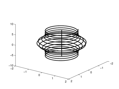
Figure 1: A schematic drawing of a helix with a gaussian deformation of the type in Eq.(26). The parameters are chosen to be $a=0.5$ and $\phi_{0}=4\phi$, and the radius then varies by a factor of $1.5$ over about $4$ windings. The length can be extended as desired.

In section II we showed that a regular helix leads to a constant effective mass. The curvature is then naturally also small or at least varying slowly with position along the one-dimensional curve. The different quantization prescriptions are then identical, except perhaps for the one-dimensional adiabatic approximation of the three-dimensional result. To emphasize the effects of varying mass and curvature we therefore start by modifying the simple helix. We keep the circular nature, that is the radial variation of the $x$ and $y$-directions are chosen to be identical, but varying quickly over a few windings. The unrelated $z$-direction is linear to maintain the equidistant helix structure. In total, we choose the parametrization in Eq. (1) to be

$$\begin{split}f_{x}(\phi)&=f_{y}(\phi)=\left(1+a\cdot\exp(-\phi^{2}/\phi_{0}^{2})\right).\\ f_{z}(\phi)&=\phi\;,\end{split}$$ (26)

where $a$ and $\phi_{0}$ are constants. For practical convenience we use the gaussian to describe the form of the variation. The size of $a$ determines the radial changes, ranging from $R$ to $R(1+a)$ and back again as $\phi$ varies from $-\infty$ to $+\infty$. The width of the gaussian, $\phi_{0}$, determines how quickly the radial change is taking place, that is over how many windings. The length of the curve is chosen to be from $\phi_{min}=-40$ to $\phi_{max}=40$, which is sufficient to allow a bump extending over several windings while the radius return to the initial value at the end points, that is when $f_{x}(\phi)=f_{y}(\phi)\approx R$. In numbers, $\phi_{0}=2\pi$ means very fast variation over one winding. A given multiplum, $\ell$, of $2\pi$ then implies the gaussian variation over $2\ell$ windings. The geometric structure is illustrated schematically in fig. 1.

Figure 2: Mass and corresponding derivatives as function of angle, $\phi$, for the parametrization in Eq.(26). Top: $m(\phi)$ (red), $10\cdot m^{\prime}(\phi)$ (green), $10\cdot m^{\prime\prime}(\phi)$ (blue), all in units of $m_{0}R^{2}$. Bottom contains potentials in units of $\frac{\hbar^{2}}{4m_{0}R^{2}}$ that enter different quantization prescriptions: $-\big{(}m^{\prime\prime}-\frac{3}{2}\frac{m^{\prime 2}}{m}\big{)}/m^{2}$(magenta), $\big{(}m^{\prime\prime}-2\frac{m^{\prime 2}}{m}\big{)}/m^{2}$(cyan), $-\kappa^{2}/2+0.1$(black), see Eqs.(13), (III.1) and (17).

The parametrization in Eq.(26) leads immediately from Eq.(4) to an effective mass given by

$$m(\phi)=m_{0}R^{2}\left(1+\left(\frac{\partial f_{x}}{\partial\phi}\right)^{2}+f_{x}^{2}\right)\;.$$ (27)

The first and second order derivatives of the mass are then easily written down along with the potentials entering the expressions for the different quantizations, that is Eqs.(13), (III.1) and (17). We show their angular dependence in fig. 2.

The mass is constant for angles far away from the bulge on the circular helix. It exhibits a gaussian peak at the center with a width of $2\phi_{0}$ in accordance with Eq.(27). This is then the origin of a non-constant mass on the quantization, or equivalently the effect from quantal motion in a one-dimensional curved space.

The size of the effects is reflected in the variation of the derivatives shown in the same figure. Both first and second derivatives are rather small implying that the different quantizations at least qualitatively should reveal the same most important features. This is in spite of the initial periodic parameterization where all such traces have disappeared since $f_{x}=f_{y}$ and the square of the sine and cosine functions are added with equal amplitude.

The differences in quantization are quantified by the three potentials at the bottom of fig. 2. For $H_{EM_{1}}$ we have the potential appearing in Eq.(13) after removal of the first order operator derivative. This term has an attractive minimum at the bulge and symmetric repulsive maxima in the tail of the bulge. The difference between $H_{EM_{1}}$ and $H_{EM_{2}}$ is comparable in size and almost flat over the bulge with two symmetric extremum points in the tail.

The transverse-mode adiabatic approximation quantization from Eq.(20) has two additional potentials compared to $H_{EM_{1}}$, that is one very similar to Eq.(III.1) and the qualitatively different geometric potential proportional to the square of the curvature. The latter is always attractive and of much larger magnitude, but otherwise with the same behavior as the mass itself, that is strongest in the center and vanishing outside the bulge, see fig. 2.

IV.2 Spectra

We now solve the schrödinger equation numerically for the given parametrization for all the different choices of quantization described in section III. We maintain the boundary conditions corresponding to a curve of finite length and fixed end-points, that $\Psi(\phi_{min})=\Psi(\phi_{max})=0$. We discretize the angular space by choosing a grid, computing the finite element representation of the operators, and diagonalizing in the corresponding basis. We then compare eigenvalues and eigenfunctions from the different quantization prescriptions.

Figure 3: The absolute energies of the four lowest states of one particle on a wire parametrized in Eq. (26) with $a=1$ and $\phi_{0}=4\pi$. The energies are in units of $\hbar^{2}/(R^{2}m_{0})$. The upper panel shows the energies of $H_{EM_{1}}$ and $H_{EM_{2}}$ where as the lower one shows the energies of $H_{geo}$

Table 1: The lowest four eigenvalues for different hamiltonians describing one particle on a wire parametrized in Eq. (26) with $a=1$ and $\phi_{0}=4\pi$. The ground state energies are in absolute values in units of $\hbar^{2}/(R^{2}m_{0})$. The excited states are reported as excitation energies related to the corresponding ground state energy. .

Hamiltonian	$H_{EM_{1}}$	$H_{EM_{2}}$	JWKB	$H_{geo}$	JWKB (including $V_{geo}$)
Ground state	$3.58\cdot 10^{-4}$	$1.63\cdot 10^{-4}$	$2.88\cdot 10^{-4}$	$-2.89\cdot 10^{-2}$	$-2.76\cdot 10^{-2}$
1st excited	$7.18\cdot 10^{-4}$	$1.02\cdot 10^{-3}$	$8.64\cdot 10^{-4}$	$8.62\cdot 10^{-6}$	$0$
2nd excited	$2.24\cdot 10^{-3}$	$2.42\cdot 10^{-3}$	$2.30\cdot 10^{-3}$	$5.07\cdot 10^{-3}$	$7.10\cdot 10^{-3}$
3rd excited	$4.29\cdot 10^{-3}$	$4.37\cdot 10^{-3}$	$4.32\cdot 10^{-3}$	$5.34\cdot 10^{-3}$	$7.10\cdot 10^{-3}$

Table 2: The same as in table 1 for $a=0.5$ and $\phi_{0}=4\pi$. .

Hamiltonian	$H_{EM_{1}}$	$H_{EM_{2}}$	JWKB	$H_{geo}$	JWKB (including $V_{geo}$)
Ground state	$3.72\cdot 10^{-4}$	$2.73\cdot 10^{-4}$	$3.34\cdot 10^{-4}$	$-2.96\cdot 10^{-2}$	$-2.86\cdot 10^{-2}$
1st excited	$9.01\cdot 10^{-4}$	$1.10\cdot 10^{-3}$	$1.00\cdot 10^{-3}$	$2.07\cdot 10^{-4}$	$0$
2nd excited	$2.65\cdot 10^{-3}$	$2.70\cdot 10^{-3}$	$2.67\cdot 10^{-3}$	$3.14\cdot 10^{-3}$	$1.70\cdot 10^{-3}$
3rd excited	$4.97\cdot 10^{-3}$	$5.03\cdot 10^{-3}$	$5.01\cdot 10^{-3}$	$4.76\cdot 10^{-3}$	$3.90\cdot 10^{-3}$

Inspection of the energies in tables 1 and 2 and figure 3 reveal a clear pattern as all hamiltonians exhibit rather similar spectra, except for the ones with geometric potential terms. We emphasize that the tables give absolute values for the ground state energies, and for better comparison the excitation energies are given for the excited states.

Let us first consider the hamiltonians without the additional geometric potential. Both absolute values and excitation energies for $H_{EM_{1}}$ and $H_{EM_{2}}$ deviate from each other by at most 50% and the JWKB approximation always assume intermediate values. All three energy sets approach each other with increasing excitation energy in accordance with an approach towards the validity of classical physics.

The simplest results are from the analytic JWKB approximation which precisely is the $n^{2}$ spectrum from a one-dimensional square well. We know from Eq. (24) that an overall energy scale is the square of the inverse length of the wire. This is seen as a constant ratio of $1.160$ for JWKB energies of the same state. Applying this scaling from the JWKB approximation on the $H_{EM_{1}}$ and $H_{EM_{2}}$ spectra show the expected decreasing deviations for increasing excitation energies. These similarities already at the lowest energies are due to the relatively small coordinate variation of the effective mass.

Including the geometric potential leads to substantially different spectra. This potential is overall attractive with constant curvature outside the bulge region in the center. The curvature and the attraction is smaller in the central region. This has strong implications on the resulting spectra where the lowest four states considered here all turn out to have negative energies. In figure 3 one sees how for larger $a$ the states turns into two sets of degenerate states. This is because of the barrier in the geometric potential that shows up for larger $a$.

Both JWKB and full solutions with the geometric potential have doubly degenerate ground states. This is due to the separation in two regions through the less attractive central peak of the geometric potential. There is room for bound states in each region, and no distinction between odd and even parity states. This is highlighted by the classically forbidden central region which is crucial for the simple JWKB solution. A better approximation would allow some tunneling into this barrier region and the degeneracies would be lifted as indicated by the energies from the full solutions.

The influence of the geometric potential is much larger than the variation between the $H_{EM_{1}}$ and $H_{EM_{2}}$ spectra. This applies for both absolute and relative energies and independent of the bulge parameter $a$. In the limit of vanishing $a$ the curvature approach a coordinate independent constant and the geometric potential becomes consequently constant as well. This amounts to a shift of all energies without any structural changes. The excitation spectra would thus approach each other.

IV.3 Eigenfunctions

Figure 4: Top: Ground state wave functions for the different choices of Hamiltonian, Eq.(15) (red), Eq.(11) (green) Eq.(25) (black), Eq.(20) (blue). The constants in the parametrization are chosen to be $a=1$ and $\phi_{0}=4\pi$. Bottom: The effective potentials for $H_{EM_{2}}$ (red) and $H_{geo}$ (blue) for the curve in Eq.(26) with $a=1$ and $\phi_{0}=4\pi$

The complete picture requires spectra supplemented by corresponding eigenfunctions. The ground state wavefunctions for the parameter choice $a=1$ and $\phi_{0}=4\pi$ are shown in fig. 4 for the different hamiltonians. All the solutions must vanish at the end of the wire, since this is the imposed boundary conditions.

Let us again first consider the cases without geometric potential. The ground state solutions are all symmetric around the center where the radius is largest and the largest probabilities occur as peaks. The solutions to $H_{EM_{1}}$ in Eq. (11) and the JWKB result from Eq (V.1) are almost indistinguishable. The probability distributions are rather broad and extending far beyond the bulge in the central region of the curve. The solution for $H_{EM_{2}}$ in Eq. (15) is rather similar although distinguishable with a central peak, slightly higher and correspondingly narrower.

The difference between the $H_{EM_{1}}$ and $H_{EM_{2}}$ solutions arises from the potential in Eq. (III.1), $\frac{\partial^{2}}{\partial\phi^{2}}\left(\frac{1}{m(\phi)}\right)$, which is plotted in fig. 2. This potential is zero at both ends, becomes repulsive when moving towards the center from either side of the potential, and finally it turns attractive in the center. The wavefunction exhibits a sharp upwards turn when the attraction is felt with the result of a larger maximum than for $H_{EM_{1}}$.

Inclusion of the geometric potential changes qualitatively all the derived solutions. The full numerical solution to $H_{geo}$ is still symmetric but with an almost vanishing minimum in the center and two prominent maxima on either side. This behavior is a direct reflection of the properties of the geometric potential shown in fig. 2 and contained in $H_{geo}$. The JWKB solution now has two separated classically allowed regions, of course provided the energies are below the barrier in the center. The simplest JWKB solutions are then zero in the central forbidden region as seen in fig. 4. The deviation from the full solution is therefore very striking but uninteresting since the probabilities at the same time are very small. An improved JWKB solution could be designed by use of an exponentially decreasing wave function to describe tunneling into the barrier.

Figure 5: First excited states for the different choices of Hamiltonian, Eq.(15) (red), Eq.(11) (green), Eq.(25) (black). The constants in the parametrization are chosen to be $a=1$ and $\phi_{0}=4\pi$.

The first excited states are shown in fig. 5 for the different hamiltonians. The boundary conditions of zero at the end points of the wire are maintained in all cases. Now a node appears in the center, and all wave functions are of odd parity. The solutions without geometric potential are almost indistinguishable for the $H_{EM_{1}}$, $H_{EM_{2}}$, solutions and the related JWKB approximation. They all resemble the sine wave functions for the first excited state of a particle in a square well potential. Now the central attraction for $H_{EM_{2}}$ is much less effective due to the required node for $\phi=0$.

Again including the geometric potential changes the solutions substantially, although much less than for the ground state. The odd parity characteristics with a central node is maintained but now with a small oscillatory modulation by tunneling into the barrier. The two regions of large probability are pushed further away from the center by the potential than the $H_{EM_{1}}$ and $H_{EM_{2}}$ solutions. The slope of the wave functions is also not as steep across the central region.

The corresponding simplest JWKB solution is trying to mimic this behavior in the classically allowed regions. The central forbidden region has a constant probability of zero. The only difference between first excited and ground state is that the ground state is even, and the first excited state is odd. The absolute values corresponding to the probability distributions would be identical.

Figure 6: Top: Ground states for the different choices of Hamiltonian, Eq.(15) (red), Eq.(11) (green), Eq.(25) (black). The constants in the parametrization are chosen to be $a=0.5$ and $\phi_{0}=4\pi$. Bottom: The effective potentials for $H_{EM_{2}}$(red) and $H_{geo}$(blue) for the curve in Eq.(26) with $a=0.5$ and $\phi_{0}=4\pi$

The dependence of the eigenfunctions on the parameters of the gaussian central bump is intuitively clear with the detailed knowledge we accumulated from the investigated set. The effects from varying the two parameters, $a$ and $\phi_{0}$, seems to be very different. The value of $aR$ is directly the radial extension of the bump beyond initial helix radius. It is therefore clear that increasing $a$ from zero must increase the change of the solutions from the $a=0$ solutions where both mass and curvature are constants. However, the qualitative behavior of even and odd parity is maintained, and with the related maxima or nodes at the center.

The $\phi_{0}$ variation appears to be very different but the effects are actually rather similar. Large values imply a slow variation of the radius of the helix, and as such small influence on the wave functions beyond a possible scaling from a different average radius. Small $\phi_{0}$ values imply fast variation over few windings. Both mass and curvature would then vary much faster as well, and the different quantizations would be very different.

Thus, large $a$ and small $\phi_{0}$ lead to large variation in mass and curvature and consequently the different quantization prescriptions would deviate more and more from each other. This would be particularly prominent in comparison with use of the geometric potential. It is worth to emphasize that it is not obvious which quantization procedure is most correct for these one-dimensional cases.

On one hand the simple JWKB approximation provides a very accurate match with the $H_{EM_{1}}$ solutions. However, this assumes that no potential is necessary to confine the particle to the one-dimensional wire. On the other hand, some geometric potential combined with an appropriate kinetic energy operator would directly deliver the hamiltonian. Unfortunately, this assumes a computational scheme to obtain a reliable potential, and the lowest order curvature dependent potential is not accurate for helix like periodic structures with strongly varying effective mass.

V Stretched helix

In contrast to the previous section we shall here investigate asymmetric helix deformations. We design here two stretching parameterizations originating from very different assumptions. We first describe these parameterizations, and in the following subsections we present results for spectra and eigenfunctions for the different quantization descriptions.

V.1 Parameterizations

We want to study the non-trivial cases where both mass and curvature are monotonously varying with the coordinate. Instead of symmetry we choose an increasing stretching along the symmetry axis of the helix, that is

$$f_{x}(\phi)=f_{y}(\phi)\;\;,\;\;f_{z}(\phi)=a\phi^{2}\;,$$ (28)

where $a$ is a constant. This curve is circular in the $x-y$ plane and the distance between the windings increase with the angle, $\phi$, see fig. 7. The effective mass is simple, that is

$$m(\phi)=m_{0}R^{2}\left(1+4a^{2}\phi^{2}\right)\;,$$ (29)

which allow analytical integration of the square root in Eq. (23), and therefore a fully analytic JWKB-solution. Only first and second derivatives are finite and expansion in higher order derivatives are more likely to converge than for a periodic structure.

Explicitly we get the bound state wave function given by Eq. (25) with

$$L(\phi)=R\left(\frac{1}{4a}\ln{\left[\frac{\phi+\sqrt{\phi^{2}+\frac{1}{4a^{2}}}}{\phi_{min}+\sqrt{\phi_{min}^{2}+\frac{1}{4a^{2}}}}\right]}\right.$$

$$\left.+a\phi\sqrt{\phi^{2}+\frac{1}{4a^{2}}}-a\phi_{min}\sqrt{\phi_{min}^{2}+\frac{1}{4a^{2}}}\right)\;,$$ (30)

where $L(\phi_{max})$ is the length of the wire.

The two hamiltonians $H_{EM_{1}}$ and $H_{EM_{2}}$ differ by the second derivative of the inverse mass, see Eq. (III.1). We can find a parametrization where this difference vanishes. The assumption of identical circles in the $x-y$ plane, $f_{x}=f_{y}=1$, gives an effective mass from Eq. (4), $m(\phi)=m_{0}R^{2}(1+(f^{\prime}_{z})^{2})$. If we therefore assume that $H_{EM_{1}}=H_{EM_{2}}$ then $1/(1+(f^{\prime}_{z})^{2})$ should be a first order polynomium i $\phi$, or equivalently $m(\phi)=\frac{1}{c_{0}+c_{1}\phi}$, where $c_{0}$ and $c_{1}$ are constants.

Figure 7: Schematic drawings of two deformed helices with stretched and squeezed parametrizations Eqs. (29) and (31). The stretching and squeezing parameters are chosen to be $a=0.1$, and $c_{0}=c_{1}=0.01$.

Integrating $f^{\prime}_{z}(\phi)$ to find $f_{z}(\phi)$, we get the parametrization:

$$f_{x}(\phi) = f_{y}(\phi)=1$$

$$f_{z}(\phi) = -\frac{\arctan{\left[\frac{-2c_{0}-2c_{1}\phi+1}{2\sqrt{-\left(c_{0}+c_{1}\phi-1\right)\left(c_{0}+c_{1}\phi\right)}}\right]}}{2c_{1}}$$ (31)

$$- \frac{2R\sqrt{-\left(c_{0}+c_{1}\phi-1\right)\left(c_{0}+c_{1}\phi\right)}}{2c_{1}}\;.$$

The curves in Eqs. (29) and (31) are different types of monotonous deformations in the z-direction. The resulting deformed helices are both shown in fig. 7.

Figure 8: Mass and corresponding derivatives as function of angle, $\phi$, for the parametrization in eq.(28). Top: $m(\phi)$ (red), $\cdot m^{\prime}(\phi)$ (green), $\cdot m^{\prime\prime}(\phi)$ (blue), all in units of $m_{0}R^{2}$. Bottom contains potentials in units of $\frac{\hbar^{2}}{4m_{0}R^{2}}$ that enter different quantization prescriptions: $-\big{(}m^{\prime\prime}-\frac{3}{2}\frac{m^{\prime 2}}{m}\big{)}/m^{2}$(magenta), $\big{(}m^{\prime\prime}-2\frac{m^{\prime 2}}{m}\big{)}/m^{2}$(cyan), $-\kappa^{2}/2$(black), see Eqs.(13), (III.1) and (17).

Figure 9: Mass and corresponding derivatives as function of angle, $\phi$, for the parametrization in eq.(31). Top: $m(\phi)$ (red), $\cdot m^{\prime}(\phi)$ (green), $\cdot m^{\prime\prime}(\phi)$ (blue), all in units of $m_{0}R^{2}$. Bottom contains potentials in units of $\frac{\hbar^{2}}{4m_{0}R^{2}}$ that enter different quantization prescriptions: $-\big{(}m^{\prime\prime}-\frac{3}{2}\frac{m^{\prime 2}}{m}\big{)}/m^{2}$(magenta), $\big{(}m^{\prime\prime}-2\frac{m^{\prime 2}}{m}\big{)}/m^{2}$(cyan), $-\frac{1}{16}\kappa^{2}/2$(black), see Eqs.(13), (III.1) and (17).

The first and second order derivatives of the mass are then easily calculated. We show their angular dependence in figs. 8 and 9 and as well the expressions in Eqs.(13), (III.1) and (17) that enters the expressions for the different quantizations. The two parameterizations can be viewed as stretching and squeezing, respectively. The structure variations in these quantities are therefore rather similar, except that they appear at small or large $\phi$, respectively as seen in figs. 8 and 9.

The mass itself increases quadratically or decreases inversely proportional with $\phi$. This smooth dependence is then the origin of the effects of this type of non-constant mass on the quantization. The different combinations are then very trivial as for example both $m^{\prime\prime}$ and $m^{\prime 2}/m$ are constants. The difference between $H_{EM_{1}}$ and $H_{EM_{2}}$ therefore quickly vanishes with $\phi$ in the first case while by construction identically equal to zero in the last case. The different combinations exhibit the opposite behavior with $\phi$. The additional potential in Eq.(20) is very small for both parameterizations. On the other hand, the geometric potential is again very decisive with prominent minima at either small or large values of $\phi$.

Table 3: The lowest four eigenvalues for different hamiltonians describing one particle on a wire parametrized in Eq. (28) with $a=0.1$ and $\phi$ varying between $\phi_{min}=0$ and $\phi_{max}=20$. The ground state energies are in absolute values in units of $\hbar^{2}/(R^{2}m_{0})$. The excited states are reported as excitation energies related to the corresponding ground state energy.

Hamiltonian	$H_{EM_{1}}$	$H_{EM_{2}}$	JWKB	$H_{geo}$	JWKB (including $V_{geo}$)
Ground state	$2.72\cdot 10^{-3}$	$1.57\cdot 10^{-3}$	$2.29\cdot 10^{-3}$	$-1.51\cdot 10^{-2}$	$-6.01\cdot 10^{-3}$
1st excited	$7.00\cdot 10^{-3}$	$6.59\cdot 10^{-2}$	$6.85\cdot 10^{-3}$	$1.69\cdot 10^{-2}$	$7.46\cdot 10^{-3}$
2nd excited	$1.84\cdot 10^{-2}$	$7.72\cdot 10^{-2}$	$1.84\cdot 10^{-2}$	$2.63\cdot 10^{-2}$	$1.70\cdot 10^{-2}$
3rd excited	$3.43\cdot 10^{-2}$	$9.31\cdot 10^{-2}$	$3.44\cdot 10^{-2}$	$4.11\cdot 10^{-2}$	$3.19\cdot 10^{-2}$

Table 4: The same as table 3 for the parametrization Eq. (31) with $c_{0}=c_{1}=0.01$ and $\phi$ varying between $\phi_{min}=0$ and $\phi_{max}=40$.

Hamiltonian	$H_{EM_{1}}$	$H_{EM_{2}}$	JWKB	$H_{geo}$	JWKB (including $V_{geo}$)
Ground state	$3.93\cdot 10^{-4}$	$3.93\cdot 10^{-4}$	$4.22\cdot 10^{-4}$	$-8.99\cdot 10^{-3}$	$-6.99\cdot 10^{-3}$
1st excited	$1.26\cdot 10^{-3}$	$1.26\cdot 10^{-3}$	$1.27\cdot 10^{-3}$	$6.23\cdot 10^{-3}$	$5.25\cdot 10^{-3}$
2nd excited	$3.37\cdot 10^{-3}$	$3.37\cdot 10^{-3}$	$3.38\cdot 10^{-3}$	$9.23\cdot 10^{-3}$	$7.38\cdot 10^{-3}$
3rd excited	$6.32\cdot 10^{-3}$	$6.32\cdot 10^{-3}$	$6.34\cdot 10^{-3}$	$1.17\cdot 10^{-2}$	$9.77\cdot 10^{-3}$

V.2 Spectra

In tables 3 and 4 we show the lowest four states of the excitation spectra of each hamiltonian. The $H_{EM_{1}}$ and $H_{EM_{2}}$ energies for both parameterizations are very close to the corresponding JWKB spectra where the differences almost disappear for the highest excited states. The deviation is largest between the absolute values of the ground state energies of the $H_{EM_{1}}$ and $H_{EM_{2}}$ hamiltonians. The largest differences between the parameterizations can be removed by the length scaling which is cleanly expressed by the analytic JWKB expression in Eq. (24).

Inclusion of the geometric potential changes the spectra substantially. This potential is attractive and able to support one or two bound state with negative energy, respectively for the two parameterizations. These features are also found in the corresponding JWKB spectra. Furthermore, the JWKB excitation energies are approached for higher excitations. The length scaling is not appropriate here, since the wave functions are pulled into the attraction regions which eliminate the importance of the finite size confinement.

V.3 Eigenfunctions of stretched helix

Figure 10: Ground states for the different choices of hamiltonian, Eq.(15) (red), Eq.((11) (green), Eq.(25) (black) for the parametrization in Eq.(28). The constants in the parametrization are chosen to be $a=0.1$.

The stretched helix is parametrized by Eq. (28) where we choose again the stretching parameter $a$ to have the value $a=0.1$. The parametric angle interval for the curve is $\phi$ varying between $\phi_{min}=0$ and $\phi_{max}=20$. The ground state wavefunctions for all the different hamiltonians are shown in fig. 10. The solution to $H_{EM_{1}}$ and $H_{EM_{2}}$ and the corresponding JWKB result all exhibit a single maximum shifted from the center at $\phi=10$ towards higher values of $\phi$. These wave functions are very similar, although that of $H_{EM_{1}}$ has the maximum shifted a little more than the almost indistinguishable results for $H_{EM_{2}}$ and the JWKB approximation. These shifts are towards higher values of the effective mass and all due to the corresponding increase with $\phi$.

The geometric potential has a very strong effect. The ground state wavefunctions still only have one peak, but now shifted towards smaller values of $\phi$, where the curvature is larger and the attraction therefore stronger. The corresponding JWKB solution is similar with one peak at roughly the same position as the full solution. However, the classically forbidden region of $V_{geo}(\phi)>E$ starts at $\phi=10$, after which the JWKB wavefunction is zero by definition.

Figure 11: Excited states for the different choices of hamiltonian, Eq.(15) (red), Eq.((11) (green), Eq.(25) (black) for the parametrization in Eq.(28). The constants in the parametrization are chosen to be $a=0.1$.

The wavefunctions for the first excited state are shown in fig. 11, where the necessary node is the prominent feature. Again almost quantitative agreement within the two groups of results, that is between the $H_{EM_{1}}$, $H_{EM_{2}}$ and related JWKB results, and between the $H_{geo}$ and corresponding JWKB results. The added geometric potential changes the quantitative behavior by moving the peaks towards smaller $\phi$-values where the attraction is largest.

V.4 Eigenfunctions of squeezed helix

Figure 12: Ground states for the different choices of hamiltonian, Eq.(15) (red), Eq.((11) (green), Eq.(25) (black) for the parametrization in Eq.(28). The constants in the parametrization are chosen to be $c_{0}=0.01$ and $c_{1}=0.01$ .

The squeezed helix, which is parameterized by Eq. (31), is designed to give $H_{EM_{1}}=H_{EM_{2}}$. The effective mass decreases with $\phi$ as $m(\phi)=\frac{1}{c_{0}+c_{1}\phi}$, where we choose $c_{0}=c_{1}=0.01$ and a curve parametrized by $\phi$ varying between $\phi_{min}=0$ and $\phi_{max}=40$. We show the ground state wavefunctions in fig. 12. They are almost a left-right reflection of the stretched wave functions in fig. 10. The overlapping wavefunctions of $H_{EM_{1}}$ and $H_{EM_{2}}$ rise quickly from zero to a single maximum at $\phi=9$, before they linearly fall off to $0$ at $\phi_{max}$. The JWKB solution is similar and rises from $0$ to a maximum at $\phi=12$, before it falls off to zero at $\phi_{max}$.

Again the geometric potential moves the peak to the opposite end of the allowed $\phi$ interval, that is to about $\phi=32$. The corresponding JWKB solution is similar with a maximum at roughly the same $\phi$ value. The decrease is steeper towards the classically forbidden region for $\phi<22$. Thus the picture is that the geometric potential move the solutions to the large curvature region, which is the opposite of the large effective mass region where the $H_{EM_{1}}$ and $H_{EM_{2}}$ solutions are peaked.

Figure 13: First excited states for the different choices of hamiltonian, Eq.(15) (red), Eq.((11) (green), Eq.(25) (black) for the parametrization in Eq.(28). The constants in the parametrization are chosen to be $c_{0}=0.01$ and $c_{1}=0.01$ .

The first excited states of the same configuration are shown in figure 13. They all now have the required node for an excited state. The overlapping solutions from $H_{EM_{1}}$ and $H_{EM_{2}}$ rise to their first maximum at $\phi=4$, then they have a node at $\phi=11$, and then a smaller minimum at $\phi=23$. The related JWKB solutions is similar with slightly shifted extremum points. The geometric potential leads to a wavefunction with a broad peak at the center, and a smaller minimum at the position where the ground state wavefunction is peaked. This is required by orthogonality. The corresponding JWKB solution is similar but has as usual to vanish within the classical forbidden region for $\phi<10$.

VI Discussion and outlook

We start with two different approaches to a system of a single particle trapped in an effective one dimensional trap. The first approach is to build a classical description of the system, and through that find an appropriate quantization. Because we allowed this one dimensional trap to have a changing curvature, this quantization step is not trivial and we show two equally valid choices, which differ only by a potential term.

The other approach starts from a quantum mechanical description in three dimensions, and then through a transverse-mode adiabatic approximation reduce to an effective one dimensional model but now with an extra so-called geometric potential. This potential is attractive and given as proportional to the square of the curvature. We then investigate three different perturbations of a helix, and calculate the wavefunctions and energies of the different hamiltonians.

Monotonous deformation results in monotonous effective mass and curvature dependence on the coordinate. However, these two key quantities behave differently and lead to opposite effects on the quantized solutions. Specifically, increasing curvature leads to increasing attraction along the wire, and therefore the ground state wavefunctions would peak at this end. Increasing effective mass also tend to move the largest probability in the same direction of large mass. This implies that the different quantization prescriptions in this case of monotonous helix deformation produce very different results.

The more periodic type of helix deformation leads to more similar quantized results although still with substantial differences. The periodic nature of a helix prohibits that the confining potential is obtained by a converged Taylor expansion in terms of the parametrizing one-dimensional path. It also strongly indicates the same problem with a quantization obtained by forced, explicit symmetrization of a non-hermitian hamiltonian. The only hamiltonian without these problems has the inverse effective mass between the two derivatives in the kinetic energy operator.

The authors acknowledge inspiring conversations with J. Stockhofe and A. Rauschenbeutel. This work was supported by the Danish Council for Independent Research.

References

- (1) Ricardez-Vargas I and Volke-Sepúlveda K 2010 J. Opt. Soc. Am. B 27 948
- (2) Reitz D and Rauschenbeutel A 2012 Opt. Commun. 285 4705
- (3) Arnold A S 2012 Optics Lett. 37 2505
- (4) MacDonald M P et al 2002 Opt. Commun. 201 21
- (5) Bhattacharya M 2007 Opt. Commun. 279 219
- (6) Sagué G, Baade A and Rauschenbeutel A 2008 New J. Phys. 10 113008
- (7) Pang Y K et al 2005 Opt. Express 13 7615
- (8) Law K T and Feldman D E 2008 Phys. Rev. Lett. 101 096401
- (9) Huhtamäki J A M and Kuopanportti P 2010 Phys. Rev. A 82 053616
- (10) Schmelcher P 2011 Europhys. Lett. 95 50005
- (11) Zampetaki A V, Stockhofe J, Krönke S and Schmelcher P 2013 Phys. Rev. E 88 043202
- (12) Pedersen J K, Fedorov D V, Jensen A S and Zinner N T 2014 J. Phys. B:At. Mol. Opt. Phys. 47 165103
- (13) Schrödinger E 1926 Ann. Physik 80 489
- (14) Hofmann H and Dietrich K 1971 Nucl. Phys. A165 1
- (15) Pauli H C and Ledergerber T 1974 Proc. Phys. and Chem. of fission IAEA Rochester, New York, 463
- (16) Brack M, Damgaard J, Jensen A S, Pauli H C, Strutinsky V M and Wong C Y 1972 Rev. Mod. Phys. 44 320.
- (17) Stockhofe J and Schmelcher P 2014 Phys. Rev. A 89 033630
- (18) Taylor J R 2005 Classical Mechanics (University Science Books)
- (19) L. Dekar, L. Chetouani, and T.F. Hammann 1999 Phys. Rev. A 59 107
- (20) do Carmo M P 1976 Differential Geometry of Curves and Surfaces (Prentice-Hall)