Tunable Anderson metal-insulator transition in quantum spin-Hall insulators

Abstract

We numerically study disorder effects in Bernevig-Hughes-Zhang (BHZ) model, and find that Anderson transition of quantum spin-Hall insulator (QSHI) is determined by model parameters. The BHZ Hamiltonian is equivalent to two decoupled spin blocks that belong to the unitary class. In contrast to the common belief that a two-dimensional unitary system scales to an insulator except at certain critical points, we find, through calculations scaling properties of the localization length, level statistics, and participation ratio, that a possible exotic metallic phase emerges between a QSHI and a normal insulator phases in InAs/GaSb-type BHZ model. On the other hand, direct transition from a QSHI to a normal insulator is found in HgTe/CdTe-type BHZ model. Furthermore, we show that the metallic phase originates from the Berry phase and can survive both inside and outside the gap.

I Introduction

Topological insulators (TI), which are identified as a class of quantum state of matter, have generated intensive interests recently. Hasan2010 ; Qi2011 The two dimensional (2D) TI, i.e., quantum spin-Hall insulator (QSHI), is characterized by odd pairs of counter propagate gapless edge states. Kane-Mele2005 ; BHZ2006 The QSHI was firstly realized in HgTe/CdTe quantum well (QW) BHZ2006 ; Konig2007 and subsequently in InAs/GaSb QW.Liu2008 ; Du2013 These two experimentally realized QSHI systems can both be represented by the inverted bands Bernevig-Hughes-Zhang (BHZ) model but with different parameters. Specifically, the coupling strength between two inverted bands in InAs/GaSb QW is an order of magnitude smaller than that of HgTe/CdTe QW. Considering the remarkable parameter difference, one open question remains, namely whether this difference will have some physical consequences in these two QSHI systems.

The Anderson metal-insulator transition in 2D disordered system manifests as a lasting research issue in condensed-matter physics.Huckestein1995 ; Kramer1993 ; Belitz1994 ; Kramer1981 ; Kramer1983 ; Anderson1979 ; Mirlin2008 Generally, the disordered electron systems can be classified into three universality ensembles according to the random matrix theory.Beenakker1997 ; Mirlin2008 In the presence of time-reversal symmetry (TRS), the system is classified as an orthogonal ensemble if spin rotation symmetry is preserved; otherwise, it belongs to a symplectic ensemble. In contrast, when the TRS is broken, the system turns into a unitary ensemble.Beenakker1997 ; Mirlin2008 For a TRS QSHI with Rashba spin orbital coupling (SOC), the system falls into the symplectic ensemble because spin rotation symmetry is broken. In contrast, without Rashba SOC, the QSHI is divided into two spin species of quantum anomalous Hall (QAH) systems, which belong to the unitary ensemble. Previous studies on metal-insulator transition in a QSHI can be summerized into two paradigms: (i) for (symplectic) QSHI with Rashba SOC, it was found that TI and normal insulator (NI) phases are separated by a metallic phase;Yamakage2011 ; Yamakage2013 ; Onoda2007 (ii) for a (unitary) QSHI without Rashba SOC, a direct transition from a TI to a NI was discovered.Yamakage2011 ; Yamakage2013 ; Onoda2007 ; Onoda2003 Surprisingly, recently a crossover from weak localization to weak anti-localization (WAL) is suggested in the BHZ model without Rashba SOC.Tkachov2011 ; Ostrovsky2012 ; Krueckl2012 Since WAL can add a positive correction to the $\beta$ function,Anderson1979 ; Hikami1980 ; Lee1985 there is the possibility that a metallic phase might exist in the 2D unitary system (QSHI) with weak disorder, although that is against the traditional view.

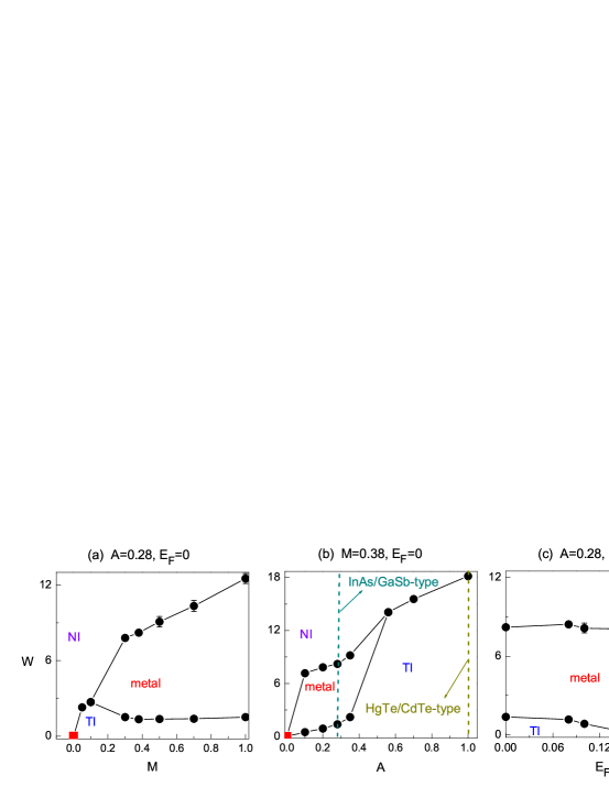
Figure 1: (Color online). The phase diagrams for disorder strength $W$ and (a) topological mass $M$, (b) electron-hole hybrid strength $A$, and (c) Fermi energy $E_{F}$. The black filled circles are critical points determined by finite size scaling, while the red filled squares for $W=0$ are analytic critical points. In (b), the dark cyan dash lines (InAs/GaSb-type BHZ parameter) indicates the TI-metal-NI transition. The dark yellow dash lines (HgTe/CdTe-type parameter) shows direct NI-TI transition.

In this paper, we study whether a metallic phase can exist between TI and NI phases in a unitary QSHI system. Starting from the BHZ model Hamiltonian,BHZ2006 ; Liu2008 we calculate the localization length and two-terminal conductance numerically, and we analyze the scaling behavior of the system.Datta ; Kramer1983 It is worth noting that the BHZ Hamiltonian is equivalent to two decoupled spin blocks which belong to the unitary class. The main results are summarized in the phase diagrams in Fig. 1. In all these phase diagrams, we find a metallic phase between TI and NI phases, in contrast to the common view of Anderson transition behavior in a 2D unitary class. Furthermore, we find that different parameters in BHZ model (unitary system) can lead to different Anderson transition behaviors. The transition from a TI to a metal is likely to exist in InAs/GaSb-type BHZ model but not in the HgTe/CdTe-type BHZ model [see dash lines in Fig. 1(b)]. By employing the Berry phase, the parameter-dependent metallic phase can be well explained.Krueckl2012 ; Tkachov2013

The rest of the paper is organized as follows. In Sec. II, we introduce the lattice model Hamiltonian and give the details of numerical simulations. In Sec. III, we show the main results by scaling of the localization length and the conductance. We discuss energy level statistics and participation ratios of eigenstates in Sec. IV. In Sec.V, we discuss the phase diagram and interpret our numerical results by the Berry phase. In Sec.VI, a brief summary is presented.

II Model and methods

We consider the disorder BHZ Hamiltonian on a square lattice:BHZ2006 ; Liu2008 ; Jiang2009

$$H = \sum_{i}\varphi_{i}^{\dagger}E_{i}\varphi_{i}^{{\vphantom{\dagger}}}+\sum_{i,\alpha=x,y}\varphi_{i}^{\dagger}T_{\alpha}\varphi_{i+\widehat{\alpha}}^{{\vphantom{\dagger}}}+H.C.,$$ (1)

with

$$E_{i} = (C-\frac{4D}{a^{2}}+V_{i})\sigma_{0}\otimes\tau_{0}+(M-\frac{4B}{a^{2}})\sigma_{0}\otimes\tau_{z},$$

$$T_{x} = \frac{D}{a^{2}}\sigma_{0}\otimes\tau_{0}+\frac{B}{a^{2}}\sigma_{0}\otimes\tau_{z}-\frac{iA}{2}\sigma_{z}\otimes\tau_{x},$$

$$T_{y} = \frac{D}{a^{2}}\sigma_{0}\otimes\tau_{0}+\frac{B}{a^{2}}\sigma_{0}\otimes\tau_{z}+\frac{iA}{2a}\sigma_{0}\otimes\tau_{y}.$$ (2)

Here $i=(i_{x},i_{y})$ is the site index, and $\widehat{\alpha}$ is the unit vector along $\widehat{\alpha}=(x,y)$ direction. $\varphi_{i}$ represents the four annihilation operators of an electron on site $i$. The model parameters $A$, $B$, $C$, and $D$ can be experimentally controlled and $a$ is the lattice constant. Specifically, two important physical parameters are coupling strength between inverted bands $A$ and the mass $M$. $\sigma$ and $\tau$ are Pauli matrices in spin and orbital spaces, respectively. We consider the long-range disorder potential $V_{i}$ at $\vec{r_{i}}$ with $V_{i}=\sum_{n=1}^{N_{I}}U_{0}\exp[-|\vec{r_{n}}-\vec{r_{i}}|^{2}/(2\xi^{2})]$, where $U_{0}$ is uniformly distributed in $(-W/2,W/2)$ with disorder strength $W$ and $N_{I}$ impurities are randomly located among $N$ lattices at {$\vec{r}_{1},\vec{r}_{2},...,\vec{r}_{N_{I}}$}.Zhang2009 ; Lewenkopf2008 ; Rycerz2007 ; Wakabayashi2007 We fix the impurity density $n=N_{I}/N=5\%$ and the disorder range $\xi=2a$, where different $n$ and $\xi$ will not significant influence our results. Since the two spin block are decoupled, we only consider the spin-up block in the rest of the paper. Because one spin species of QSHI is a QAH insulator, our results in this paper are applicable to the QAH or Chern Insulator.

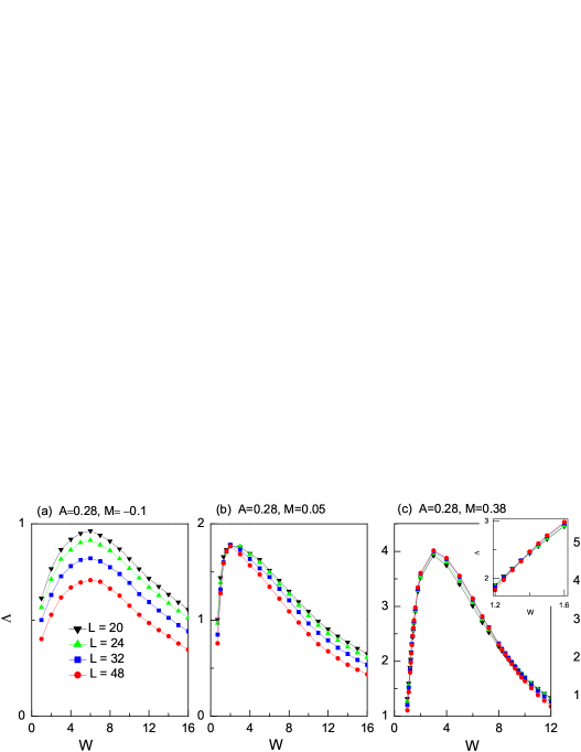
Figure 2: (Color online). (a)-(d) renormalized localization length $\Lambda=\lambda_{L}/L$ versus disorder strength $W$ for different masses $M$ and widths $L$ with fixed Fermi energy $E_{F}=0$. The inset of (c) and (d) are the zoom-in of the critical point on left side of main panel of (c) and (d), respectively.

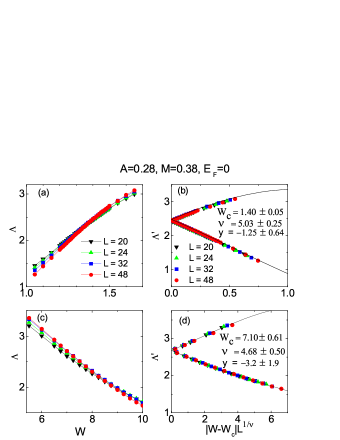
Figure 3: (Color online). (a) and (c) shows $\Lambda=\lambda_{L}/L$ vs disorder strength $W$ near two critical points. The parameters are the same as those of Fig. 2(c). (b) and (d) are single parameter scaling of $\Lambda$ in (a) and (c), respectively. $\nu$ is the critical exponent at critical disorder strength $W_{c}$.

In our numerical calculations, we study the localization length $\lambda_{L}$ as well as the dimensionless intrinsic conductance $g$ of the cylindrical sample with width (circumference) $L$,Jiang2009 which can eliminate the effect of the helical edge states. $g$ is defined as $1/g=1/g_{L}-1/N$, with $g_{L}$ the two-terminal conductance and $N$ the number of propagating channels.Braun ; Zhang2009 ; Slevin The localization length $\lambda_{L}$ of the sample is calculated by transfer-matrix method Kramer1983 with the sample’s length $10^{6}$ to $10^{7}$. The two terminal conductance $g_{L}$ at Fermi energy $E_{F}$ is evaluated by the Landauer-Büttiker formulaDatta ; Braun ; Zhang2009 with a disordered middle region with size $L\times L$ being considered as coupled to two clean semi-infinite leads. In addition, we also investigate the energy level statistics as well as participation ratios. For simplicity, the parameters $B=1$, $C=0$, $D=0$, and $a=1$ are fixed in the rest of paper, where we have assumed the particle-hole symmetry ($D=0$).

III Metal-insulator transition

First, we study $\Lambda=\lambda_{L}/L$ versus disorder strength $W$ by increasing the mass from $M=-0.1$ to $0.5$ at a fixed Fermi energy $E_{F}=0$, as shown in Fig. 2. These parameters resemble the InAs/GaSb QW $k\cdot p$ parameters.note1 Notably, we find the TI-metal-NI transition in the InAs/GaSb-type BHZ model (unitary system) by increasing the mass $M$. In the NI phase with $M<0$, $\Lambda=\lambda_{L}/L$ decreases monotonously with increasing $L$ in Fig.2(a) which indicates all the states are localized. In contrast, when $M=0.05$ in TI phase ($M>0$), the system shows one critical (touching) point where $\Lambda$ is independent of $L$ [see Fig.2(b)], which is consistent with the previous studies of a 2D unitary system.Onoda2003 ; Onoda2007 ; Yamakage2013 Due to the inverted gap, the TI is robust to weak disorder, and the NI phase appears after a certain disorder strength $W_{c}=2.3\pm 0.13$. Therefore, this critical (touching) point indicates a direct transition from NI to TI. Surprisingly, in Fig. 2(c), when the mass $M$ is increased to $0.38$, the metallic phase ($\Lambda$ increasing with $L$) appears between $W_{c1}\approx 1.40$ [see the inset of Fig. 2(c)] and $W_{c2}\approx 7.10$. This metallic phase is contradict to the common behavior of the 2D unitary class. The unitary system, e.g., quantum Hall system, is scaled to localized states except at certain critical (touching) points. Moreover, upon further increasing $M$, the metallic phase region becomes larger, i.e., for $M=0.5$, the metallic phase remains in Fig. 2(d) between $W_{c1}\approx 1.40$ [see inset of Fig. 2(d)] and $W_{c2}\approx 8.2$. This peculiar metallic phase between the TI and NI phases in the InAs/GaSb-type BHZ model is the main finding of our paper.

Next, we analyze the one parameter scaling behavior of the renormalized localization length $\Lambda=\lambda_{L}/L$ near the critical points of Fig. 2(c). According to finite size scaling law, all $\Lambda$ are fitted to $\Lambda(W,L)=\Lambda_{c}+\sum^{4}_{n=1}a_{n}(W-W_{c})^{n}L^{n/\nu}+b_{0}L^{y}$ near the critical point, Kramer1981 ; Kramer1983 ; Kramer1993 ; Slevin1997 ; Onoda2007 ; Obuse2007 where $W_{c}$ is the disorder strength at a critical point, $\nu$ is critical exponent and $y$ is an exponent associated with the leading irrelevant operator. Here, $a_{n}$ and $b_{0}$ are the fitting parameters. For convenience, we define $\Lambda^{\prime}(W,L)=\Lambda(W,L)-b_{0}L^{y}$, with the same parameters as $\Lambda$. The best fit is given by minimizing $\chi^{2}$ statistic $\chi^{2}=\sum_{n=1}^{N}(\Lambda_{n}-\Lambda(W_{n},L_{n}))^{2}/\sigma_{n}^{2}$, where $N$ is the number of the data and $\sigma_{n}$ is the error of the $n$th data $\Lambda_{n}$. The finding of the metallic phase and the large critical exponent $\nu$ (almost twice as large as that obtained previously) in Figs.3(c) and (d) suggests the existence of a possible new universality class.Onoda2003 ; Asada2002 ; Slevin2009 ; Huckestein1990 We caution that the standard deviations ($\chi^{2}/N$) are $3.3$ and $3.5$ for Figs.3(b) and (d), respectively, which are somewhat larger than the common value unity and even larger size computations are desirable to obtain a high precision critical exponent $\nu$.

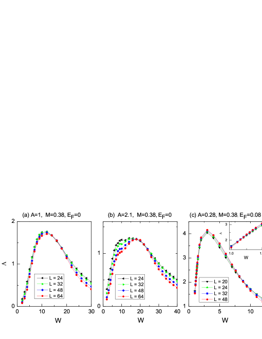
Figure 4: (Color online). (a)-(d) $\Lambda=\lambda_{L}/L$ versus disorder strength $W$. The parameters are shown on top of each panel. The inset of (c) shows a zoom-in of the critical point on the left side in the main panel. The inset of (d) shows average intrinsic conductance $\langle g\rangle$ of square sample versus $W$ with same model parameters as (d).

Up to now, we have found the metallic phase for small $A=0.28$, which resembles the parameters of InAs/GaSb-type BHZ model. To compare with previous studies,Yamakage2011 ; Yamakage2013 it is necessary to investigate Anderson transition for large $A$ cases, i.e., the HgTe/CdTe-type BHZ model. In Figs. 4 (a) and (b), where $M=0.38$ and $E_{F}=0$, $A$ increases from $1$ to $2.1$, in the region of the HgTe/CdTe-type model parameters. The other parameters are the same as those of Fig. 2(c). Compared with the case $A=0.28$ [see Fig. 2(c)], the metallic phase disappears for $A=1$ and $A=2.1$ because $\Lambda$ hardly changes with the size near the touching point [see Figs. 4(a) and (b)]. This direct transition from TI to NI (i.e. $A=~{}1,~{}2.1$) is consistent with previous study in the HgTe/CdTe-type BHZ model.Yamakage2011 ; Yamakage2013 Meanwhile, the localization length decreases rapidly with increasing $A$ from $0.28$ to $2.1$. For example, for a typical unitary case $A=1$, the localization length $\lambda_{L}$ is only $1\sim 2$ times of width of the system $L$. From the above results, it is natural to conclude that the existence of the metallic phase is highly dependent on the magnitude of $A$. To be specific, the transition TI-metal-NI in the InAs/GaSb-type BHZ model is absent in the HgTe/CdTe-type BHZ model.

Now we consider the influence of Fermi energy $E_{F}$ on the metallic phase. In Fig. 4(c), when $A=0.28$, $M=0.38$, and $E_{F}=0.08$ in the neighborhood of the gap center, the transition TI-metal-NI remains almost the same as that of Fig. 2(c) with $E_{F}=0$. When the Fermi energy is moved outside the band gap $E_{g}\simeq 0.16$, i.e., $E_{F}=0.17$, the transition from metal to NI is still observed by scaling $\Lambda$ and $\langle g\rangle$ in Fig. 4(d). It is clear that $\langle g\rangle$ and $\Lambda$ increase with the size of the system in the metallic phase, they decrease in insulator phase, and there is a crossing point ($W\approx 8$) at the phase transition. To conclude, the localization length scaling and the conductance scaling suggest that the metallic phase could survive both inside and outside the band gap.

IV energy level statistics and participation ratio

Figure 5: (Color online). (a) solid blue line is the variances of the energy spacing distributions at different energies $E_{F}$ with the disorder strength $W=4$. The red dash line indicates the variances of Wigner surmise of unitary ensemble. (b)–(i) The histograms of nearest energy level spacings centered at different energies $E_{F}=0$–$8$ with $W=4$. The solid red lines and green lines represent Wigner surmise of unitary ensemble and Poisson distribution, respectively. The model parameters are $A=0.28$ and $M=0.38$ with the sizes $48\times 48$.

Furthermore, we have verified the existence of the metallic phase by studying the energy level statistics and evaluating the participation ratio of eigenstates. According to the random matrix theory, the delocalized and localized states can be characterized by the energy level statistics.Mehta ; Mirlin2008 In Fig.5, the histograms of the level spacings are drawn at different energies $E_{F}$. The sizes is $48\times 48$ with a periodical boundary condition in two directions, i.e., a torus geometry.Prodan2010 ; Song2014 In the energy region $E_{F}=0$–$0.2$, the histograms [see Fig.5(b)-(d)] and corresponding variances [see Fig.5(a)] are very close to those of the Wigner surmise of a unitary ensemble $p(s)=(32/\pi^{2})s^{2}\exp[-(4/\pi)s^{2}]$.Mehta Therefore, the level correlation is long-ranged which indicates that extend states may exist. However, near the top of the band ($E=8$) [see Fig.5(i)], the histogram is close to the Poisson distribution $p(s)=\exp(-s)$, which implies that the states are uncorrelated and localized.

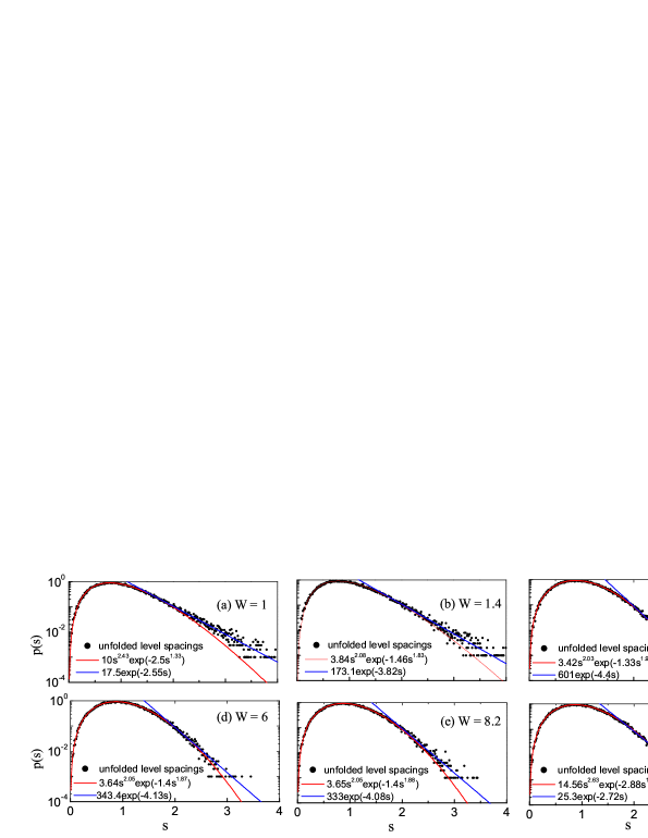
Figure 6: (Color online). Distributions of the unfolded level spacings $s$ under different disorder strength (a) $W=1$ to (f) $W=12$ are fitting by Wigner surmise $p(s)=As^{\alpha}\exp(Bs^{\beta})$ for whole $s$ region and Poisson distribution $p(s)=A\exp(Bs)$ for $s>2$. The model parameters are $A=0.28$ and $M=0.38$ at $E_{F}=0$.

However, in the histograms of the level spacings, it is difficult to distinguish the critical point ( or region) from the true metallic phase, because they are both close to Wigner surmise of the unitary class. To identify the true metallic phase, we test the larger sized ($L\times L=128\times 128$) results at fixed energy $E_{F}=0$ with different disorder strength $W=1$–$12$. Then we fit the distributions to Wigner surmise $p(s)=as^{\alpha}\exp(bs^{\beta})$ for the whole $s$ region and Poisson distribution $p(s)=k\exp(\kappa s)$ for $s>2$, with the fitting parameter $\alpha$ ($\beta$, $\kappa$) and the renormalization parameter $a$ ($b$, $k$).Wang1998 The fitting error of a set of data $\{\bar{p}(s_{1}),\bar{p}(s_{2}),...,\bar{p}(s_{N})\}$ is defined as $\sigma^{2}=\sum_{i=1}^{N}[p(s_{n})/\bar{p}(s_{n})-1]^{2}/N$, where $p(s_{n})$ is the fitting value at $s_{n}$ and $N$ is the number of data. It is noted that if energy level spacings data follows the Wigner surmise with $\alpha=2$ and $\beta=2$, a metallic phase exits; however, if the data only follows this distribution in the small $s$ region but violates in the large-$s$ region, the critical behavior emerges. Shklovskii1993 ; Wang1998

Figure6 shows a logarithmic plot of $p(s)$ for the distributions of the unfolded level spacings $s$.footnote2 In Figs.6(c) and (d), for $W=4$ and $6$ the fitting parameters $\alpha$ and $\beta$ are very close to the Wigner surmise of the unitary ensemble, $\alpha=\beta=2$. Therefore, the level correlation is long ranged. On the other hand, for $W=1.4$ and $8.2$ [see Fig.6(b) and (e)], although the fitting parameters $\alpha$ and $\beta$ are very close to the Wigner surmise of the unitary ensemble, the large $s$ region is not well described by the Wigner surmise. Instead, the tail of the large $s$ region is clearly fitted to Poisson distribution. The hybrid of the Wigner surmise statistics and Poisson statistics behavior at a critical point is coincident with the level statistics results at the 3D Anderson metal-insulator transition.Shklovskii1993 In this case, the level correlation is finite-ranged, which manifests as a crossing over from (long-ranged correlated) Wigner surmise statistics to (uncorrelated) Poisson statistics. For $W=1$ and $W=12$ [see Fig.6(a) and (f)], the level spacings clearly deviated from the Wigner surmise of the unitary ensemble for the whole $s$ region and the energy levels will become totally uncorrelated in thermodynamic limit, identifying an insulating phase. In conclusion, the level statistics results strongly support the existence of a metallic phase between $W=4$ and $W=6$ at $E_{F}=0$. This is coincident with the region indicated by finite size scaling results of localization length (see Fig.1).

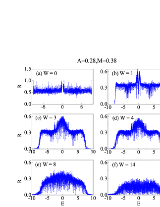
Figure 7: (Color online). The participation ratio R as functions of energy E at the disorder strength (a)$W=0$ to (f) $W=14$ at the size $48\times 48$.

The participation ratio characterized the spatial extension of the eigenstates. Next, we will investigate the participation ratio under different disorder strength. The participation ratio is defined as $R=\sum_{i=1}^{N}|a_{i}|^{4}/(N\sum_{i=1}^{N}|a_{i}|^{2})^{2}$ where $a_{i}$ is the wave function at lattices $i$ and $N$ is the number of the lattice. Edwards1972 ; Bauer1990 ; Zhang2009 ; Murphy2011 $R$ has its maximum $1$ for one single Bloch wave, reaches a finite value typical around $1/3$ for a disordered extended state, and approaches $\sim 1/N$ for a localized state. In Fig.7(b) and (c), the (highly possible) extended states characterized by the peaks $R\approx 0.6$ are found near the bulk gap at $W=1$, and then come into the gap upon increasing the disorder strength $W=3$. As a result, the metallic phase in the gap indeed comes from the extended states near the gap, which originates from the nearly $\pi$ Berry phase. At last, the peak of $R$ diminishes upon increasing the disorder strength [see Fig.7(d)-(f)] which indicates that the states are localized at $W=14$ ($R<1/3$).

V Phase diagram and discussion

We summarize our results into three phase diagrams: $W$-$M$, $W$-$A$, and $W$-$E_{F}$, as shown in Fig. 1. In Fig. 1(a), the metallic phase emerges from TI phase at $M\simeq 0.1$ and expands with increasing $M$ from $0.1$ to $1$. On the other hand, in Fig. 1(b), the metallic phase exists for small A cases and disappears for $A>0.56$. In other words, the transition TI-metal-NI can exist in the InAs/GaSb-type BHZ model but not in the HgTe/CdTe-type BHZ model [see the dash lines in Fig.1(b)]. Furthermore, in Fig. 1(c), the metallic phase spreads over both inside and outside the gap ($E_{g}=0.16$). The phase diagram Fig. 1(c) indicates that the metallic phase inside and outside the gap have the same physical origin.

In a 2D system, the metal phase is related to WAL, which adds the positive correction to the $\beta$ function and leads to such phase in the thermodynamic limit. Anderson1979 ; Lee1985 ; Imura2009 In general, the WAL exists in SOC systems of a symplectic ensemble,Hikami1980 and Dirac systems with a $\pi$ Berry phase, e.g., graphene and helical surface states of 3D TI.McCann2006 ; Lu2011 In the present case, the detailed analysis of symmetry classes and Berry phases can help us to understand the peculiar metallic phase in the inverted band BHZ model. We first analyze the symmetry classes of the BHZ model. The spin-$\uparrow$ part of the BHZ Hamiltonian in momentum space is $H_{0}(k)=A(k_{x}\tau_{x}+k_{y}\tau_{y})+(M-Bk^{2})\tau_{z}$, where $A,B,M$ and $\tau$ have the same meaning as in Eq. (2). When the mass term $M-Bk_{F}^{2}=0$, the system satisfies pseudo-time reversal symmetry, i.e., $H_{0}(k_{F})=\tau_{y}H_{0}^{*}(-k_{F})\tau_{y}$, which is similar to the massless Dirac particles in graphene. Therefore, the system is approximate symplectic and shows WAL in the region near $M-Bk_{F}^{2}=0$.Tkachov2011 ; Ostrovsky2012 On the contrary, when $|M-Bk_{F}^{2}|>>A|k_{x}+ik_{y}|$, the two orbital bands are nearly decoupled, thus the system belongs to orthogonal ensemble approximately and shows weak localization.Tkachov2011 ; Ostrovsky2012 Therefore, the existence of the metallic phase is dependent on the system parameters. Moreover, the Berry phase of the BHZ model at Fermi energy $E_{F}$ reads: Krueckl2012 ; Tkachov2013

$$\gamma(E_{F})=(1-\frac{(M-Bk_{F}^{2})}{\sqrt{A^{2}k_{F}^{2}+(M-Bk_{F}^{2})^{2}}})\pi,$$ (3)

where $k_{F}$ is the momentum at $E_{F}$. The Berry phase $\gamma$ monotonously increases with $k_{F}$ rising from zero. $\gamma=0$ at $k_{F}=0$, $\gamma=\pi$ at $k_{F}=\sqrt{M/B}$, and $\gamma\rightarrow 2\pi$ while $k_{F}$ tends to $\infty$. Since $\gamma$ can vary from 0 to $2\pi$, the system can show both WAL and weak localization which depends on the parameters. While $M/B>>A^{2}/B^{2}$, $k_{g}=\sqrt{\frac{M}{B}-\frac{A^{2}}{2B^{2}}}\simeq\sqrt{M/B}$, where $k_{g}$ is the momentum at the conduction-band bottom and the valence-band top, and then the Berry phase $\gamma\simeq\pi$. In this case, the system exhibits WAL and the metallic phase exists between TI and NI phases (see Fig. 1). For the case of the InAs/GaSb-type BHZ model, i.e., $A=0.28$, $B=1$, and $M=0.38$, $M/B>>A^{2}/B^{2}$ is well satisfied, the metallic phase consequently appears. In contrast, for the HgTe/CdTe type model, i.e., $A=1$, $B=1$, and $M=0.38$ with $M/B<A^{2}/B^{2}$, $k_{g}=0$ which is far away from $\sqrt{M/B}$. At $k_{g}=0$, the Berry phase $\gamma=0$, which leads the weak localization behavior and the disappearance of the metallic phase.

VI Discussion and Conclusion

The Berry phase argument is well applicable to the present numerical simulations and it is also in accordance with previous investigations. Tkachov2011 ; Ostrovsky2012 When the system is “approximate symplectic”, electrons interfere as a symplectic system on the length scalings smaller than $l_{M}=v_{F}\tau_{M}$. Here $v_{F}$ is the Fermi velocity, $\tau_{M}=\frac{\tau}{2}(A^{2}k_{F}^{2}+(M-Bk_{F}^{2})^{2})/(M-Bk_{F}^{2})^{2}$ is the TRS-breaking scattering time and $\tau$ is the elastic scattering time.Tkachov2011 ; Ostrovsky2012 In this case, $l_{M}$ acts as large-size cufoff for WAL correction resembling the dephasing length, and the WAL correction dominates if system width $L<<l_{M}$.Tkachov2011 ; Ostrovsky2012 In our numerical simulation, for example, when $E_{F}=0.17$ in Fig.4(d), $l_{M}=v_{F}\tau_{M}=l_{s}\tau_{M}/\tau\sim 300$, where the mean free path $l_{s}\sim\sqrt{1/n}\sim 4$ and $\tau_{M}/\tau\sim 75$. Here we have used the impurity density $n=5\%$ and the Fermi vector $k_{F}\sim 0.605$. Since $l_{M}>>L$ the system width in the numerical simulations, the TRS-breaking scattering time $\tau_{M}$ is not important and the system resembles symplectic with metallic behaviors. This metallic behavior can show up in mesoscopic systemsPikulin2014 and may apply to recent transport experiments Du2013 . For larger systems with $L>L_{M}$, the scaling behavior should be interesting, however this is beyond our present numerical capability, and thus is left for further study.

In summary, we investigated the Anderson metal-insulator transition in QSHI and found different localization behaviors depending on model parameters. Notably, the transition TI-metal-NI likely exists in InAs/GaSb-type systems but not in HgTe/CdTe-type systems. The peculiar metallic phase, which originates from the Berry phase $\pi$ near the band gap, contradicts the common view of the Anderson transition behavior of the 2D unitary class.

VII Acknowledgements

This work was financially supported by NBRP of China (2015CB921102,2012CB921303, 2012CB821402, and 2014CB921901) and NSF-China under Grants Nos. 11274364, NO. 91221302 and No. 11374219. ZW is supported by DOE Basic Energy Sciences grant DE-FG02-99ER45747. H.J. is supported by the NSF of Jiangsu province BK20130283.

References

- (1) M. Z. Hasan and C. L. Kane, Rev. Mod. Phys. 82, 3045 (2010).
- (2) X.-L. Qi and S.-C. Zhang, Rev. Mod. Phys. 83, 1057 (2011).
- (3) C. L. Kane and E. J. Mele, Phys. Rev. Lett. 95, 226801 (2005).
- (4) A. Bernevig, T. Hughes, and S. C. Zhang, Science 314, 1757 (2006).
- (5) M. König, S. Wiedmann, C. Brüne, A. Roth, H. Buhmann, L. Molenkamp, X.-L. Qi, and S.-C. Zhang, Science 318, 766 (2007).
- (6) C. Liu, T. L. Hughes, X.-L. Qi, K. Wang, and S.-C. Zhang, Phys. Rev. Lett. 100, 236601 (2008).
- (7) L. Du, I. Knez, G. Sullivan, and R.-R. Du, Phys. Rev. Lett. 114, 096802 (2015).
- (8) E. Abrahams, P. W. Anderson, D. C. Licciardello, and T. V. Ramakrishnan, Phys. Rev. Lett. 42, 673 (1979).
- (9) A. MacKinnon and B. Kramer, Phys. Rev. Lett. 47, 1546 (1981).
- (10) A. MacKinnon and B. Kramer, Z. Phys. B 53, 1 (1983).
- (11) B. Kramer and A. MacKinnon, Rep. Prog. Phys. 56, 1469 (1993)
- (12) D. Belitz and T. R. Kirkpatrick, Rev. Mod. Phys. 66, 261 (1994).
- (13) B. Huckestein, Rev. Mod. Phys. 67, 357 (1995).
- (14) F. Evers and A. D. Mirlin, Rev. Mod. Phys. 80, 1355 (2008).
- (15) C. W. J. Beenakker, Rev. Mod. Phys. 69, 731 (1997).
- (16) M. Onoda, Y. Avishai, and N. Nagaosa, Phys. Rev. Lett. 98, 076802 (2007).
- (17) A. Yamakage, K. Nomura, K. I. Imura, and Y. Kuramoto, J. Phys. Soc. Jpn. 80, 053703 (2011).
- (18) A. Yamakage, K. Nomura, K.-I. Imura, and Y. Kuramoto, Phys. Rev. B 87, 205141 (2013).
- (19) M. Onoda and N. Nagaosa, Phys. Rev. Lett. 90, 206601 (2003).
- (20) G. Tkachov and E. M. Hankiewicz, Phys. Rev. B 84, 035444 (2011).
- (21) P. M. Ostrovsky, I. V. Gornyi, and A. D. Mirlin, Phys. Rev. B 86, 125323 (2012).
- (22) V. Krueckl and K. Richter, Semicond. Sci. Technol. 27, 124006 (2012).
- (23) S. Hikami, A. I. Larkin, and Y. Nagaoka, Prog. Theor. Phys. 63, 707 (1980).
- (24) P. A. Lee and T. V. Ramakrishnan, Rev. Mod. Phys. 57, 287 (1985).
- (25) S. Datta, Electronic Transport in Mesoscopic Systems (Canmbridge University Press, Cambridge, England, 1995).
- (26) G. Tkachov, Phys. Rev. B 88, 205404 (2013).
- (27) H. Jiang, L. Wang, Q.-F. Sun, and X. C. Xie, Phys. Rev. B 80, 165316 (2009). J.-C. Chen, J. Wang, and Q.-F. Sun, ibid. 85, 125401 (2012).
- (28) A. Rycerz, J. Tworzydło, and C. W. J. Beenakker, Europhys. Lett. 79, 57003 (2007).
- (29) K. Wakabayashi, Y. Takane, and M. Sigrist, Phys. Rev. Lett. 99, 036601 (2007).
- (30) C. H. Lewenkopf, E. R. Mucciolo, and A. H. Castro Neto, Phys. Rev. B 77, 081410(R) (2008).
- (31) Y.-Y. Zhang, J.-P. Hu, B. A. Bernevig, X. R. Wang, X. C. Xie, and W. M. Liu, Phys. Rev. Lett. 102, 106401 (2009).
- (32) D. Braun, E. Hofstetter, G. Montambaux, and A. MacKinnon, Phys. Rev. B 55, 7557 (1997).
- (33) K. Slevin, P. Markoš, and T. Ohtsuki, Phys. Rev. Lett. 86, 3594 (2001).
- (34) The dimensionless parameters , , to correspond to meVnm, meVnm, C=0, and meV to meV, with the lattice constant nm. They are InAs/GaSb-type parameters because is about an order of magnitude smaller than that of HgTe/CdTe-type.
- (35) K. Slevin and T. Ohtsuki, Phys. Rev. Lett. 78, 4083 (1997).
- (36) H. Obuse, A. Furusaki, S. Ryu, and C. Mudry, Phys. Rev. B 76, 075301 (2007).
- (37) B. Huckestein and B. Kramer, Phys. Rev. Lett. 64, 1437 (1990).
- (38) Y. Asada, K. Slevin, and T. Ohtsuki, Phys. Rev. Lett. 89, 256601 (2002).
- (39) K. Slevin and T. Ohtsuki, Phys. Rev. B 80, 041304(R) (2009).
- (40) M. L. Mehta, Random Matrices, 2nd ed. (Academic, Boston, 1991).
- (41) E. Prodan, T. L. Hughes, and B. A. Bernevig, Phys. Rev. Lett. 105, 115501 (2010).
- (42) J. Song, C. Fine, and E. Prodan, Phys. Rev. B 90, 184201 (2014).
- (43) V. Plerou and Z. Wang, Phys. Rev. B 58, 1967 (1998).
- (44) B. I. Shklovskii, B. Shapiro, B. R. Sears, P. Lambrianides, and H. B. Shore, Phys. Rev. B 47, 11487 (1993).
- (45) The logarithmic plots (see Fig. 6) show strongly scattered data in large may be misleading. In fact,Y-axis are logarithmic, and thus the deviation in large data are small. For example, in Fig.6, the error of the Wigner surmise (red line) in large region are . The fitting parameter are mainly determinted by the large data by minimize the error .
- (46) J. T. Edwards and D. J. Thouless, J. Phys. C 5, 807 (1972).
- (47) J. Bauer, T. M. Chang and J. L. Skinner, Phys. Rev. B 42, 8121 (1990).
- (48) N. C. Murphy, R. Wortis, and W. A. Atkinson, Phys. Rev. B 83, 184206 (2011).
- (49) K.-I. Imura, Y. Kuramoto, and K. Nomura, Phys. Rev. B 80, 085119 (2009).
- (50) H. Suzuura and T. Ando, Phys. Rev. Lett. 89, 266603 (2002). E. McCann, K. Kechedzhi, V. I. Fal’ko, H. Suzuura, T. Ando, and B. L. Altshuler, ibid. 97, 146805 (2006).
- (51) H.-Z. Lu, J. Shi, and S.-Q. Shen, Phys. Rev. Lett. 107, 076801 (2011).
- (52) D. I. Pikulin, T. Hyart, Shuo Mi, J. Tworzydło, M. Wimmer, and C. W. J. Beenakker, Phys. Rev. B 89, 161403(R) (2014).