Measure on gauge invariant symmetric norms

Abstract

The concept of a gauge invariant symmetric random norm is elaborated in this paper. We introduce norm processes and show that this kind of stochastic processes are closely related to gauge invariant symmetric random norms. We construct a gauge invariant symmetric random norm on the plain. We define two different extensions of these random norms to higher (even infinite) dimensions. We calculate numerically unit spheres of expected norms in two and three dimensions for the constructed random norm.

1 Introduction

We do not need to emphasize that norms and metrics induced by norms play very important role in analysis. A norm $||.||:\mathbb{C}^{n}\to[0,\infty)$ on $\mathbb{C}^{n}$ is called gauge invariant if it satisfies the condition

$$\forall x\in\mathbb{C}^{n}\quad||x||=||\,|x|\,||$$

where $|.|$ denotes the element-wise absolute value of the vector, and it is said to be symmetryc if it satisfies the condition

$$\forall\pi\in S_{n}\,\,\forall x\in\mathbb{C}^{n}\quad||x\circ\pi||=||x||$$

where $S_{n}$ denotes the symmetric group of order $n$. Obviously, familiar $p$-norms frequently used in analysis possess these properties. Note that gauge invariant symmetric norms are determined by those on $\mathbb{R}_{+,\geq}^{n}:=\{(x_{1},\ldots,x_{n})|x_{1}\geq x_{2}\geq\ldots\geq x_{n}\geq 0\}$ [1]. All kind of norms considered in this paper has the property that the norm of the vector $(1,0,0,\ldots,0)$ is equal to $1$ which is called the normalization convention.

There are some applications when it would be useful to define a measure on gauge invariant symmetric norms which can be given on the considered vector space. These measures can be interpreted as a random norm.

Definition 1.

Let $(\Omega,\mathcal{F},\mathbb{P})$ be a probability space. A function $p:\Omega\times\mathbb{C}^{n}\to[0,\infty)$ is called gauge invariant symmetric random norm (GSRN) if the following conditions hold:

1. $\mathbb{P}\left(\left\{\omega\in\Omega\left|\,p(\omega,.):\mathbb{C}^{n}\to[0,\infty)\text{ is a symmetric gauge invariant norm.}\right.\right\}\right)=1$.

2. $\forall x\in\mathbb{C}^{n}\quad p(.,x):\Omega\to[0,\infty)$ is a random variable.

It can be easily deduced from the definition of gauge invariant symmetric norm and the normalization convention that

$$\forall x\in\mathbb{C}^{n}\quad\mathbb{P}\left(\left\{\omega\in\Omega\left|p(\omega,x)\notin[||x||_{\infty},||x||_{1}]\right.\right\}\right)=0$$ (1)

holds, and for any $x\in\mathbb{C}^{n}$ the expectation of $p(.,x)$ is a symmetric gauge invariant norm.

The paper is organized as follows. Section 2 is divided into three subsections. In subsection 2.1 and 2.2, we introduce norm processes and theirs path integral representation. In subsection 2.3, we give some basic definitions for continuous-time Markov chains and we define Markovian GSRNs. In section 3, we present an efficient tool for studying the distribution of continuous-time Markov chain time integrals and we construct a Markovian GSRN on the plain. Section 4 deals with higher dimensional generalizations of GSRNs and an open problem is presented in this section. Finally, in section 5 an application is presented.

2 GSRN on the plain

2.1 Norm processes

Obviously, a symmetric gauge invariant norm restricted to $\mathbb{R}^{2}_{+,\geq}$ can be given by its unit circle which can be parametrized by the second coordinates of points lying on it. This observation motivates the following definition.

Definition 2.

A real valued stochastic process $(X_{t})_{t\geq 0}$ is called a norm process if its realizations satisfy the following conditions $\mathbb{P}$-a.s.:

1. $X_{0}=0$,

2. $\forall\,0\leq t_{1}<t_{2}\quad 0\leq\frac{X_{t_{2}}-X_{t_{1}}}{t_{2}-t_{1}}\leq 1$ and

3. $t\mapsto X_{t}$ is convex and continuous.

The next Theorem states that norm processes can be considered as a paramerization of the unit circles restricted to $\mathbb{R}^{2}_{+,\geq}$.

Theorem 1.

Let $(X_{t})_{t\geq 0}$ be a norm process, the corresponding probability space of which is $(\Omega,\mathcal{F},\mathbb{P})$. It is true for $\mathbb{P}$-a.s. $\omega\in\Omega$ that for any $v=(v_{1},v_{2})\in\mathbb{R}^{2}_{+,\geq}\setminus\{(0,0)\}$ there is a unique $p\in\left[||v||_{\infty},||v||_{1}\right]$ such that

$$\frac{v_{1}}{p}+X_{\frac{v_{2}}{p}}(\omega)=1$$

holds and the function $p:\Omega\times\mathbb{R}^{2}_{+,\geq}\setminus\{(0,0)\}\to[0,\infty)$, which is defined for $\mathbb{P}$-a.s. $\omega\in\Omega$, extended to $0\in\mathbb{R}^{2}_{+,\geq}$ as $p(0):=0$ is a GSRN.

Proof.

Suppose that for $\omega\in\Omega$ conditions $i.-iii.$ in definition 2. are satisfied. Let $v=(v_{1},v_{2})\in\mathbb{R}^{2}_{+,\geq}\setminus\{(0,0)\}$ be an arbitrary vector. The function $(0,\infty)\ni p\mapsto\frac{v_{1}}{p}+X_{\frac{v_{2}}{p}}(\omega)$ is continuous, strictly decreasing and

$$\begin{split}\frac{v_{1}}{v_{1}}+X_{\frac{v_{2}}{v_{1}}}(\omega)&\geq 1\\ \frac{v_{1}}{v_{1}+v_{2}}+X_{\frac{v_{2}}{v_{1}+v_{2}}}(\omega)&\leq 1\end{split}$$ (2)

hold because $0\leq X_{t}\leq t$. This implies that there exists a unique $p\in\left[||v||_{\infty},||v||_{1}\right]$ for which $\frac{v_{1}}{p}+X_{\frac{v_{2}}{p}}(\omega)=1$.

Let us consider the extension of $p$ and choose an $\omega\in\Omega$ as above.

1. For all $v\in\mathbb{R}^{2}_{+,\geq}$ $p(\omega,v)=0\Leftrightarrow v=0$ because $p(\omega,v)\in\left[||v||_{\infty},||v||_{1}\right]$.

2. For all $\alpha>0$ $\frac{\alpha v_{1}}{p(\omega,\alpha v)}+X_{\frac{\alpha v_{2}}{p(\omega,\alpha v)}}=1$ hence $p(\omega,\alpha v)=\alpha p(\omega,v)$.

3. If $v,w\in\mathbb{R}^{2}_{+,\geq}$ are nonzeros vectors, then due to the convexity of $t\mapsto X_{t}(\omega)$ we have

   $$\begin{split}1&=\frac{v_{1}+w_{1}}{p(\omega,v)+p(\omega,w)}+\frac{p(\omega,v)}{p(\omega,v)+p(\omega,w)}X_{\frac{v_{2}}{p(\omega,v)}}+\frac{p(\omega,w)}{p(\omega,v)+p(\omega,w)}X_{\frac{w_{2}}{p(\omega,w)}}\\ &\geq\frac{v_{1}+w_{1}}{p(\omega,v)+p(\omega,w)}+X_{\frac{v_{2}+w_{2}}{p(\omega,v)+p(\omega,w)}}\end{split}$$

   hence $p(\omega,v+w)\leq p(\omega,v)+p(\omega,w)$.

So we have deduced that if $\omega\in\Omega$ satisfies conditions $(i)-(iii)$ in definition 2, $p(\omega,.):\mathbb{R}^{2}_{+,\geq}\to[0,\infty)$ defines a symmetric gauge invariant norm.

Let $v\in\mathbb{R}^{2}_{+,\geq}$ be an arbitrary vector and $y\in(0,\infty)$ we have

$$\mathbb{P}\left(p(.,v)<y\right)=\mathbb{P}\left(\frac{v_{1}}{y}+X_{\frac{v_{2}}{y}}<1\right)=\mathbb{P}\left(X_{\frac{v_{2}}{y}}<1-\frac{v_{1}}{y}\right)$$

which means that $p(.,v):\Omega\to\left[||v||_{\infty},||v||_{1}\right]$ is a random variable. ∎

If $y\in\left[||v||_{\infty},||v||_{1}\right]$, then $0\leq\frac{v_{2}}{y}\leq\frac{v_{2}}{v_{1}+v_{2}}\leq 1$ and $0\leq 1-\frac{v_{1}}{y}\leq 1-\frac{v_{1}}{v_{1}+v_{2}}\leq 1$. Consequently, it is enough to consider the function

$$(t,x)\mapsto\mathbb{P}\left(X_{t}(.)<x\right)$$

on $[0,1]^{2}$. Conversely, unit circles of a GSRN restrcited to $\mathbb{R}^{2}_{+,\geq}$ can be considered as graphs of a pathwise restricted norm process which cannot be identified uniquely by the GSRN.

2.2 Representation of norm processes

We have seen that norm processes are closely related to GSRNs therefore it would be desirable to find good representations of it. We know from the theory of integration that a continuous monotone function is almost all differentiable and it is equal to the integral function of its almost all existing derivative [4]. If we apply this fact to the trajectories of a norm process $(X_{t})_{t\geq 0}$, we get that there exists a process $\left(Z_{t}\right)_{t\geq 0}$ such that

$$X_{t}(.)\stackrel{{\scriptstyle\mathbb{P}\text{-a.s.}}}{{=}}\int\limits_{0}^{t}Z_{s}(.)\,\mathrm{d}s$$

and trivially the realizations of $\left(Z_{t}\right)_{t\geq 0}$ are non negative, increasing and bounded functions whose upper bound is one. Therefore, we may assume that

$$\left(Z_{t}\right)_{t\geq 0}=(\tilde{F}\circ Y_{t})_{t\geq 0}$$

where $(Y_{t})_{t\geq 0}$ is a $\mathbb{P}$-a.s. increasing stochastic process in a partially ordered metric space $(S,\leq)$ and $\tilde{F}:S\to[0,1]$ is a monotone increasing function.

$$X_{t}(.)\stackrel{{\scriptstyle\mathbb{P}\text{-a.s.}}}{{=}}\int\limits_{0}^{t}\tilde{F}\circ Y_{s}(.)\,\mathrm{d}s$$ (3)

The above introduced path integral representation suggests another representation for norm processes. If we assume that $\tilde{F}$ is a probability distribution function corresponding to a random variable $\xi\in S$ which is defined on a different probability space $(\Lambda,\mathcal{G},\tilde{\mathbb{P}})$ and we consider $\xi$ and the process $(Y_{t})_{t\geq 0}$ as random processes on $(\Omega\times\Lambda,\mathcal{F}\otimes\mathcal{G},\mathbb{P}\otimes\tilde{\mathbb{P}})$ that are independent, then we can write

$$\begin{split}X_{t}(.)\stackrel{{\scriptstyle\mathbb{P}\text{-a.s.}}}{{=}}\int\limits_{0}^{t}\tilde{F}\circ Y_{s}(.)\,\mathrm{d}s=&\int\limits_{0}^{t}\tilde{\mathbb{P}}(\xi<Y_{s})\,\mathrm{d}s=\\ =&\int\limits_{0}^{t}\int\limits_{\Lambda}1\!\!1_{\xi(\eta)<Y_{s}(.)}\,\mathrm{d}\tilde{\mathbb{P}}(\eta)\,\mathrm{d}s=\int\limits_{\Lambda}\int\limits_{0}^{t}1\!\!1_{\xi(\eta)<Y_{s}(.)}\,\mathrm{d}s\,\mathrm{d}\tilde{\mathbb{P}}(\eta)=\mathbb{E}_{\tilde{\mathbb{P}}}\left((t-\tau_{\xi}(.))_{+}\right),\end{split}$$ (4)

where $\tau_{r}$ is the hitting time of level $S\ni r$: $\tau_{r}=\inf\{s\geq 0|Y_{s}\geq r\}$.

2.3 Markovian GSRNs

Definition 3.

A GSRN is said to be Markovian if the associated norm process can be derived from a Markovian process through taking its integral in time.

Markovian GSRNs are neither trivial nor so complicated that we cannot understand their behaviour especially in cases when the state space is finite. For this reason, some elementary facts are sketched about continuous-time Markov chains. This plays just an introductory role and more information about continuous-time Markov chains can be found in [3].

Definition 4.

A stochastic process $(Y_{t})_{t\geq 0}$ on a countable state space $S$ is said to be a time homogeneous continuous-time Markov chain, if it is memoryless which means

$$\mathbb{P}\left(Y_{t}=\beta\left|Y_{t_{1}}=\alpha_{1},\ldots Y_{t_{n}}=\alpha_{n}\right.\right)=\mathbb{P}\left(Y_{t}=\beta\left|Y_{t_{1}}=\alpha_{1}\right.\right)$$

holds for each $0<t_{1},\ldots,t_{n}<t$ and for any $\alpha_{1},\ldots,\alpha_{n},\beta\in S$, there exists a mapping $P:[0,\infty)\to\mathbb{R}^{S}\times\mathbb{R}^{S}$ for which

$$\forall t\in[0,\infty)\quad\forall\alpha,\beta\in S\quad\mathbb{P}\left(Y_{t}=\beta\left|Y_{0}=\alpha\right.\right)=P(t)_{\alpha\beta}$$

holds and $P$ satisfies the following properties

1. $P(0)=\mathrm{id}_{\mathbb{R}^{S}}$

2. $\exists\lim\limits_{t\searrow 0}P(t)=\mathrm{id}_{\mathbb{R}^{S}}$

3. $P(t+s)=P(t)P(s)$ $\forall t,s\in[0,\infty)$.

For each $t\in[0,\infty)$ the matrix $P(t)$ is called transition matrix corresponding to the time point $t$.

Conditions $(i)-(iii)$ in definition above imply that there exists a unique $G\in\mathbb{R}^{S}\times\mathbb{R}^{S}$ for which $P(t)=e^{tG}$ holds and $G$ is called the infinitesimal generator of continuous-time Markov chain [3].

3 An example for GSRN

3.1 Path integral of continuous-time Markov chains

In this point path integrals of continuous-time Markov chains are taken under consideration. The next Theorem is a variant of the Feynman–Kac formula [2] for continuous-time Markov chains on finite state spaces. This will enable us to compute the distribution of Markovian GSRNs.

Theorem 2.

Let $(Y_{t})_{t\geq 0}$ be a continuous-time Markov chain on a finite state space $S$ of which the infinitesimal generator is $G$ and let $f:S\to\mathbb{R}$ be an injective function. If $(X_{t})_{t\geq 0}$ denotes the path integral process of $f\circ Y$:

$$X_{t}=\int\limits_{0}^{t}f\circ Y_{s}\,\mathrm{d}s,$$

then the characteristic function of $X_{t}$ can be expressed as follows

$$(\forall y_{0}\in S)\quad\mathbb{E}\left(e^{iuX_{t}}\left|Y_{0}=y_{0}\right.\right)=e^{t(G+iuM_{f})}(\mathbf{1})(y_{0})$$ (5)

where $\mathbf{1}:S\to\{1\}$ is the constant function and $M_{f}:\mathbb{R}^{S}\to\mathbb{R}^{S}$ is the operator of multiplication by $f$.

Proof.

The function $t\mapsto f(Y_{t}(\omega))$ is a step function for all $\omega\in\Omega$ hence its integral can be expressed as a limit of Riemann sums. Using this and the dominated convergence theorem we can write the following.

$$\begin{split}\mathbb{E}\left(e^{iuX_{t}}\left|Y_{0}=y_{0}\right.\right)=\mathbb{E}\left(\left.e^{iu\lim\limits_{m\to\infty}\frac{t}{m}\sum\limits_{k=1}^{m}f\left(Y_{\frac{kt}{m}}\right)}\right|Y_{0}=y_{0}\right)=\lim\limits_{m\to\infty}\mathbb{E}\left(\left.e^{iu\frac{t}{m}\sum\limits_{k=1}^{m}f\left(Y_{\frac{kt}{m}}\right)}\right|Y_{0}=y_{0}\right)\end{split}$$ (6)

Using the injectivity of $f$ and the Markovian property of $(Y_{t})_{t\geq 0}$ we get

$$\begin{split}\mathbb{E}&\left(\left.e^{iu\frac{t}{m}\sum\limits_{k=1}^{m}f\left(Y_{\frac{kt}{m}}\right)}\right|Y_{0}=y_{0}\right)=\sum_{y_{1},\ldots,y_{m}\in S}e^{iu\frac{t}{m}\sum\limits_{k=1}^{m}f(y_{k})}\mathbb{P}\left(\left.\bigcap\limits_{k=1}^{m}\left\{f\left(Y_{\frac{kt}{m}}\right)=f(y_{k})\right\}\right|Y_{0}=y_{0}\right)=\\ =&\sum_{y_{1},\ldots,y_{m}\in S}\prod\limits_{k=1}^{m}e^{\frac{iut}{m}f(y_{k})}\mathbb{P}\left(\left.Y_{\frac{kt}{m}}=y_{k}\right|Y_{\frac{(k-1)t}{m}}=y_{k-1}\right).\end{split}$$ (7)

Observe that the received expression can be written as the action of the $m$-times composite of the operator $e^{\frac{t}{m}G}e^{\frac{iu}{m}M_{f}}$ on $\mathbf{1}$.

$$\sum_{y_{1},\ldots,y_{m}\in S}\prod\limits_{k=1}^{m}e^{\frac{iut}{m}f(y_{k})}\mathbb{P}\left(\left.Y_{\frac{kt}{m}}=y_{k}\right|Y_{\frac{(k-1)t}{m}}=y_{k-1}\right)=\left(e^{\frac{t}{m}G}e^{\frac{iut}{m}M_{f}}\right)^{m}(\mathbf{1})(y_{0})$$

If we take the limit as $m\to\infty$ and we use the Lie–Trotter product formula we get the desired expression.

$$\mathbb{E}\left(e^{iuX_{t}}\left|Y_{0}=y_{0}\right.\right)=\lim\limits_{m\to\infty}\left(e^{\frac{t}{m}G}e^{\frac{iut}{m}M_{f}}\right)^{m}(\mathbf{1})(y_{0})=e^{t(G+iuM_{f})}(\mathbf{1})(y_{0})$$

∎

Let us introduce the following notations for the conditional characteristic function above and the corresponding conditional distribution function.

$$\begin{split}\varphi(t,u)&=\mathbb{E}\left(e^{iuX_{t}}\left|Y_{0}\right.\right)\\ F(t,x)&=\mathbb{P}\left(X_{t}<x\left|Y_{0}\right.\right)\end{split}$$ (8)

If we take the time derivative of (5) we get that $\varphi$ is the solution of the Cauchy-problem below.

$$\begin{split}\partial_{1}\varphi&=G\varphi+iuM_{f}\varphi\\ \varphi(0,u)&=\mathbf{1}\in\mathbb{R}^{S}.\end{split}$$ (9)

Let us introduce a normally distributed random variable $\xi$ which is independent from $X_{t}$ and its variance is $\sigma^{2}>0$. The characteristic function $\varphi_{\sigma}$ of $X_{t}+\xi$ satisfies equations similar to (9).

$$\begin{split}\partial_{1}\varphi_{\sigma}&=G\varphi_{\sigma}+M_{f}iu\varphi_{\sigma}\\ \varphi(0,u)&=e^{-\frac{\sigma^{2}u^{2}}{2}}\cdot\mathbf{1}\in\mathbb{R}^{S}\end{split}$$ (10)

Assume that $\partial_{1}F_{\sigma}(t,x)$ exists and vanishes for all $t\in[0,\infty)$ when $x\to-\infty$. We can write

$$\begin{split}\partial_{1}\varphi_{\sigma}(t,u)&=\frac{\partial}{\partial t}\int\limits_{\mathbb{R}}e^{iux}\,F_{\sigma}(t,\mathrm{d}x)=\frac{\partial}{\partial t}\int\limits_{\mathbb{R}}e^{iux}\,\int\limits_{[0,t]}\partial_{1}F_{\sigma}(s,\mathrm{d}x)\,\mathrm{d}s\\ &=\frac{\partial}{\partial t}\int\limits_{[0,t]}\int\limits_{\mathbb{R}}e^{iux}\,\partial_{1}F_{\sigma}(s,\mathrm{d}x)\,\mathrm{d}s=\int\limits_{\mathbb{R}}e^{iux}\,\partial_{1}F_{\sigma}(t,\mathrm{d}x),\end{split}$$ (11)

and

$$\int\limits_{\mathbb{R}}iue^{iux}\,F_{\sigma}(t,\mathrm{d}x)=\left.-\partial_{2}F_{\sigma}(t,x)e^{iux}\right|_{x=-\infty}^{x=\infty}+\int\limits_{\mathbb{R}}iue^{iux}\,F_{\sigma}(t,\mathrm{d}x)=\int\limits_{\mathbb{R}}-e^{iux}\,\partial_{2}F_{\sigma}(t,\mathrm{d}x)$$ (12)

which implies that the Fourier–Stieltjes transform of the signed Borel measure associated to $\partial_{1}F_{\sigma}-GF_{\sigma}+M_{f}\partial_{2}F_{\sigma}$ is zero

$$\forall t\in[0,\infty)\,\forall u\in\mathbb{R}\quad\int\limits_{\mathbb{R}}e^{iux}\,\left[\partial_{1}F_{\sigma}-GF_{\sigma}+M_{f}\partial_{2}F_{\sigma}\right](t,\mathrm{d}x)=0.$$ (13)

On the other hand

$$\forall t\in[0,\infty)\quad\lim\limits_{x\to-\infty}\left[\partial_{1}F_{\sigma}-GF_{\sigma}+M_{f}\partial_{2}F_{\sigma}\right](t,x)=0$$

which implies that $F_{\sigma}$ is the solution of the Cauchy problem

$$\begin{split}\partial_{1}F_{\sigma}&=GF_{\sigma}-M_{f}\partial_{2}F_{\sigma}\\ F_{\sigma}(0,x)&=\Phi_{\sigma}(x)\cdot\mathbf{1}\in\mathbb{R}^{S},\end{split}$$ (14)

where $\Phi_{\sigma}$ denotes the distribution function of $\xi$.

Remark 1.

From the integral form of $X$ we obtain the estimation

$$X_{t}+\xi+\Delta t\cdot m\leq X_{t+\Delta t}+\xi\leq X_{t}+\xi+\Delta t\cdot M,$$

where $m=\min\limits_{s\in S}f(s)$ and $M=\max\limits_{s\in S}f(s)$. Using this we get

$$F_{\sigma}(t,x-\Delta t\cdot M)\leq F_{\sigma}(t+\Delta t,x)\leq F_{\sigma}(t,x-\Delta t\cdot m)$$

which can be applied to estimate partial derivatives of $F_{\sigma}$ through estimating difference quotients as follows:

$$-M\cdot\frac{F_{\sigma}(t,x)-F_{\sigma}(t,x-\Delta tM)}{\Delta t\cdot M}\leq\frac{F_{\sigma}(t+\Delta t,x)-F_{\sigma}(t,x)}{\Delta t}\leq-m\cdot\frac{F_{\sigma}(t,x)-F_{\sigma}(t,x-\Delta t\cdot m)}{\Delta t\cdot m}$$

($\leq$ relation means elementwise relations). Consequently, upper and lower bounds were obtained for $\partial_{1}F_{\sigma}(t,x)$

$$-M\cdot\partial_{2}F_{\sigma}(t,x)\leq\partial_{1}F_{\sigma}(t,x)\leq-m\cdot\partial_{2}F_{\sigma}(t,x)$$

from which it follows that the assumption about the limit of $\partial_{1}F_{\sigma}(t,x)$ as $x\to-\infty$ can be omitted.

The random variable $X_{t}+\xi$ converges weakly to $X_{t}$ when $\sigma\to 0$ thus we have to solve (14) and take the limit $\sigma\to 0$ to obtain $F$ in all points of continuity. The following Theorem gives an integral equation representation for $F$.

Theorem 3.

If $\left(X_{t}\right)_{t\geq 0}$ is a stochastic process defined in Theorem 2, then for any $y_{0}\in S$ the conditional distribution $F(t,x)_{y_{0}}=\mathbb{P}\left(X_{t}<x\left|Y_{0}=y_{0}\right.\right)$ is the solution of the following integral equation

$$\begin{split}&F(t,x)_{y_{0}}=e^{-t\lambda}1\!\!1(x\geq t\cdot f(y_{0}))+\\ &+\int\limits_{0}^{t}\sum\limits_{\sigma\in S\setminus\{y_{0}\}}F(s,x-(t-s)\cdot f(y_{0}))_{\sigma}\cdot\mathbb{P}\left(Y_{t-s}=\sigma\left|Y_{0}=y_{0}\right.\right)\lambda e^{-\lambda(t-s)}\,\mathrm{d}s,\end{split}$$ (15)

where the time spent by $Y_{s}$ in each states has exponential distribution with $\lambda$ parameter.

Proof.

Let us denote the time up to the first jump by $\tau$. By using the law of total probability

$$F(t,x)_{y_{0}}=\mathbb{P}\left(X_{t}<x\left|Y_{0}=y_{0},\tau\geq t\right.\right)\mathbb{P}\left(\tau\geq t\right)+\int\limits_{0}^{t}\mathbb{P}\left(X_{t}<x\left|Y_{0}=y_{0},\tau=t-s\right.\right)\cdot\lambda e^{-\lambda(t-s)}\,\mathrm{d}s$$

can be written, because $\tau$ is independent from the initial state. We have $\mathbb{P}\left(X_{t}<x\left|Y_{0}=y_{0},\tau\geq t\right.\right)=1\!\!1(x-t\cdot f(y_{0})\geq 0)$. We get in a similar way

$$\mathbb{P}\left(X_{t}<x\left|Y_{0}=y_{0},\tau=t-s\right.\right)=\sum\limits_{\sigma\in S\setminus\{y_{0}\}}\mathbb{P}\left(X_{t}<x\left|Y_{0}=y_{0},Y_{t-s}=\sigma,\tau=t-s\right.\right)\cdot\mathbb{P}\left(Y_{t-s}=\sigma\left|Y_{0}=y_{0}\right.\right)$$

which is true for any $s\in[0,t)$ and due to the Markov property of $\left(Y_{t}\right)_{t\geq 0}$

$$\mathbb{P}\left(X_{t}<x\left|Y_{0}=y_{0},Y_{t-s}=\sigma,\tau=t-s\right.\right)=F(s,x-(t-s)\cdot f(y_{0}))_{\sigma}$$

can be written which completes the proof. ∎

3.2 Constuction of a GSRN

In this point we consider $(Y_{t})_{t\geq 0}$ a continuous-time Markov chain on $S=\{0,\ldots,n\}$ ($n\in\mathbb{N}$) of which the infinitesimal generator is $G=\lambda_{n}N\in\mathbb{R}^{(n+1)\times(n+1)}$ where

$$N=\left(\begin{array}[]{cccccc}-1&1&0&\cdots&0&0\\ 0&-1&1&\cdots&0&0\\ 0&0&-1&\cdots&0&0\\ \vdots&\vdots&\vdots&\ddots&\vdots&\vdots\\ 0&0&0&\cdots&-1&1\\ 0&0&0&\cdots&0&0\end{array}\right)$$

and $(\lambda_{n})_{n\in\mathbb{N}}$ regulates the “speed” of the chain. We will compute the distribution function of the integral process

$$X_{t}=\int\limits_{0}^{t}\frac{1}{n}Y_{s}\,\mathrm{d}s$$

as we presented in the previous subsection. Every piecewise linear function on $[0,\infty)$ with $n$ line segments can be realized as a trajectory of $\left(X_{t}\right)_{t\geq 0}$ thus $X_{t}$ defines a measure on gauge invariant symmetric norms which unit circles are $4n$-gons.

The Cauchy problem corresponding to the smoothed variable can be written as

$$\begin{split}\partial_{1}(F_{\sigma})_{k}+\frac{k}{n}\partial_{2}(F_{\sigma})_{k}+\lambda_{n}(F_{\sigma})_{k}&=\lambda_{n}(F_{\sigma})_{k+1}\\ \partial_{1}(F_{\sigma})_{n}+\frac{k}{n}\partial_{2}(F_{\sigma})_{n}+\lambda_{n}(F_{\sigma})_{n}&=0\\ (F_{\sigma})_{k}(0,x)&=\Phi_{\sigma}(x),\end{split}$$ (16)

where $(F_{\sigma})_{k}=\mathbb{P}(X_{t}+\xi<x|Y_{0}=k)$ and $k=0,\ldots,n$. If we substitute $(F_{\sigma}(t,x))_{k}$ by $e^{-t\lambda_{n}}(J_{\sigma}(t,x))_{k}$ we obtain a system of quasilinear partial differential equations

$$\begin{split}\partial_{1}(J_{\sigma})_{k}+\frac{k}{n}\partial_{2}(J_{\sigma})_{k}&=\lambda_{n}(J_{\sigma})_{k+1}\\ \partial_{1}(J_{\sigma})_{n}+\frac{k}{n}\partial_{2}(J_{\sigma})_{n}&=0\\ (J_{\sigma})_{k}(0,x)&=\Phi_{\sigma}(x)\end{split}$$ (17)

which can be solved directly by using methods of characteristics. We get the following recursion for $F_{\sigma}$

$$\begin{split}(F_{\sigma})_{n}(t,x)&=\Phi_{\sigma}(x-t)\\ (F_{\sigma})_{k}(t,x)&=e^{-t\lambda_{n}}\Phi_{\sigma}\left(x-\frac{k}{n}\cdot t\right)+\int\limits_{0}^{t}(F_{\sigma})_{k+1}\left(t,x-\frac{k}{n}(t-s)\right)\lambda_{n}e^{-\lambda_{n}(t-s)}\,\mathrm{d}s\\ \text{for }k&=0,\ldots,n-1.\end{split}$$ (18)

If $\sigma\to 0$ we obtain

$$\begin{split}(F)_{n}(t,x)&=1\!\!1(x-t\geq 0)\\ (F)_{k}(t,x)&=e^{-t\lambda_{n}}1\!\!1\left(x-\frac{k}{n}\cdot t\geq 0\right)+\int\limits_{0}^{t}(F)_{k+1}\left(t,x-\frac{k}{n}(t-s)\right)\lambda_{n}e^{-\lambda_{n}(t-s)}\,\mathrm{d}s\\ \text{for }k&=0,\ldots,n-1\end{split}$$ (19)

which is the same as we would got, if formula (15) have been used.

System (17) for $\sigma=0$ was solved numerically by upwind scheme [5] and then expectation of the GSRN, which is a symmetric gauge invariant norm, was computed. In simulations the interval $[0,1]$ was divided into $N+1$ equal parts by $N$ internal points. Graph of $(F)_{0}(t,x)$ is presented in Figure 1, where simulation was carried out by the following settings: $n=10$, $\lambda_{n}=10$ and $N=200$.

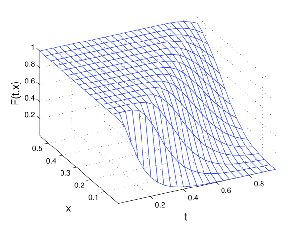
Figure 1: Probability distribution function of $X_{t}$ ($n=10$, $\lambda_{n}=10$, $N=200$).

Unit circles of the expected norm restricted to $\mathbb{R}^{2}$ can be seen in Figure 2. Two different marginal behaviour can be recognized: If $\lambda_{n}=0$, then the expected norm coincides with the maximum norm. If $\lambda_{n}\to\infty$, then the expected norm tends to the usual $1$-norm.

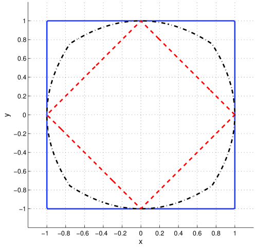
Figure 2: Unit circles of expected norms. Solid – ($n=1$, $\lambda_{n}=0$, $N=4000$), dashed – ($n=1$, $\lambda_{n}=100$, $N=500$), dash-dot – ($n=100$, $\lambda_{n}=100$, $N=1000$).

4 GSRN in higher dimensions

4.1 Strong and weak extensions

One possible way to generalize the results to higher dimensions is just using the observation that for the familiar $p$-norms $||v||_{p}=||\left(v_{1},||(v_{2},\ldots,v_{n})||\right)||_{p}$ holds for each $v=(v_{1},\ldots,v_{n})\in\mathbb{C}^{n}$. We have already constructed GSRN on $\mathbb{C}^{2}$ ($n=2$). Suppose that by induction that family of GSRNs are given on $\mathbb{C}^{k}$ where $k<n$. Let $v=(v_{1},\ldots,v_{n})\in\mathbb{R}^{n}_{+,\geq}$ be arbitrary and $\stackrel{{\scriptstyle(n-1)}}{{p}}$ is a GSRN defined on $\mathbb{C}^{n-1}$. Let $p$ be a GSRN on $\mathbb{C}^{2}$ independent from $\stackrel{{\scriptstyle(n-1)}}{{p}}$ and define $\stackrel{{\scriptstyle(n)}}{{p}}(.,v)=p\left(.,\left((v_{1},\stackrel{{\scriptstyle(n-1)}}{{p}}\left(.,(v_{2},\ldots,v_{n})\right)\right)\right)$. Of course, $\stackrel{{\scriptstyle(n)}}{{p}}$ is a gauge invariant random norm on $\mathbb{C}^{n}$, but it is not necessarily symmetric. However, the restriction of $\stackrel{{\scriptstyle(n)}}{{p}}$ to $\mathbb{R}^{n}_{+,\geq}$ defines a GSRN on $\mathbb{C}^{n}$. If $\stackrel{{\scriptstyle(n)}}{{p}}$ is a GSRN defined on $\mathbb{C}^{n}$ by using an i.i.d. sequence of the GSRN $p$ on $\mathbb{C}^{2}$, then $\stackrel{{\scriptstyle(n)}}{{p}}$ will be called the $n$-dimensional strong extension of $p$.

The main handicap of the procedure presented above is that for any $v\in\mathbb{C}^{n}$ $\stackrel{{\scriptstyle(n)}}{{p}}$ is a random variable defined on the $n$ times tensorial product of a probability space which makes simulations complicated. For this reason we define the weak extension of $p$ which is similar to the strong one just the induction step is replaced by $\stackrel{{\scriptstyle(n)}}{{p_{w}}}(.,v)=p\left(.,\left((v_{1},\mathbb{E}\left(\stackrel{{\scriptstyle(n-1)}}{{p_{w}}}\left(.,(v_{2},\ldots,v_{n})\right)\right)\right)\right)$. Unit sphere of the expected norm for $\stackrel{{\scriptstyle(3)}}{{p_{w}}}$ is presented in Figure 3, where $\stackrel{{\scriptstyle(3)}}{{p_{w}}}$ is the 3-dimensional weak extension of the GSRN presented in section 3.

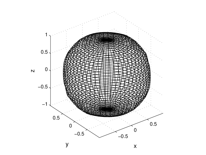
Figure 3: Unit sphere of the expected norm defined by the weak extension of the GSRN presented in section 3 ($n=100$, $\lambda_{n}=100$, $N=500$).

4.2 Open problem

Both strong and weak extensions can be generalized to infinite dimensions as the limit norms of finite dimensional truncations. Obviously, property (1) is inherited to infinite dimension hence for any $v=(v_{1},v_{2},\ldots)$ sequence of complex numbers which means $||v||_{\infty}\leq\stackrel{{\scriptstyle(\infty)}}{{p}}(v)\leq||v||_{1}$ and $||v||_{\infty}\leq\stackrel{{\scriptstyle(\infty)}}{{p_{w}}}(v)\leq||v||_{1}$ hold $\mathbb{P}$-a.s. which implies that space of sequences for which expected norm is convergent contains $l^{1}$ and it is a subspace of $l^{\infty}$. This raises many questions. For example: Let us define an equvalence relation between norm processes in the following way. Two norm processes are said to be equivalent if corresponding strong (or weak) extensions to infinite dimension define equivalent expected norms. How can be caracterized equivalence classes of this equivalence relation?

References

• [1] Rajendra Bhatia, Matrix Analysis, Springer Verlag, 1997, ISBN 0-387-94846-5.
• [2] Bernt Øksendal, Stochastic Differential Equations, Springer Verlag, 2003, 6th edition, ISBN-10 3540047581.
• [3] Yin, G. George, Zhang, Qing, Continuous-Time Markov Chains and Applications, Springer Verlag, 2013, 2nd edition, ISBN 978-1-4614-4346-9.
• [4] Paul R. Halmos, Measure Theory, Springer Verlag, 1978, ISBN-10 0387900888.
• [5] Hirsch, C., Numerical Computation of Internal and External Flows, John Wiley & Sons, 1990, ISBN 978-0-471-92452-4.