Strong stability preserving explicit linear multistep methods with variable step size

Abstract

Strong stability preserving (SSP) methods are designed primarily for time integration of nonlinear hyperbolic PDEs, for which the permissible SSP step size varies from one step to the next. We develop the first SSP linear multistep methods (of order two and three) with variable step size, and prove their optimality, stability, and convergence. The choice of step size for multistep SSP methods is an interesting problem because the allowable step size depends on the SSP coefficient, which in turn depends on the chosen step sizes. The description of the methods includes an optimal step-size strategy. We prove sharp upper bounds on the allowable step size for explicit SSP linear multistep methods and show the existence of methods with arbitrarily high order of accuracy. The effectiveness of the methods is demonstrated through numerical examples.

1 Introduction

Strong stability preserving (SSP) linear multistep methods (LMMs) with uniform step size have been studied by several authors [Len89, Len91, HRS03, RH05, HR05, Ket09]. In this work, we develop the first variable step-size SSP multistep methods.

The principal area of application of strong stability preserving methods is the integration of nonlinear systems of hyperbolic conservation laws. In such applications, the allowable step size $h_{\textup{max}}$ is usually determined by a CFL-like condition, and in particular is inversely proportional to the fastest wave speed. This wave speed may vary significantly during the course of the integration, and its variation cannot generally be predicted in advance. Thus a fixed-step-size code may be inefficient (if $h_{\textup{max}}$ increases) or may fail completely (if $h_{\textup{max}}$ decreases).

SSP Runge–Kutta methods are used much more widely than SSP LMMs. Indeed, it is difficult to find examples of SSP LMMs used in realistic applications; this may be due to the lack of a variable step-size (VSS) formulation. Tradeoffs between Runge–Kutta and linear multistep methods have been discussed at length elsewhere, but one reason for preferring LMMs over their Runge–Kutta counterparts in the context of strong stability preservation stems from the recent development of a high-order positivity preserving limiter [ZS10]. Use of Runge–Kutta methods in conjunction with the limiter can lead to order reduction, so linear multistep methods are recommended [GKS11, ZS10].

There exist two approaches to variable step-size multistep methods [HNW93]. In the first, polynomial interpolation is used to find values at equally spaced points, and then the fixed-step-size method is used. In the second, the method coefficients are varied to maintain high order accuracy based on the solution values at the given (non-uniform) step intervals. Both approaches are problematic for SSP methods; the first, because the interpolation step itself may violate the SSP property, and the second, because the SSP step size depends on the method coefficients. Herein we pursue the second strategy.

The main contributions of this work are:

• sharp bounds on the SSP coefficient of variable step-size SSP LMMs (Theorems 2-4);

• optimal methods of orders two and three (Sections 3.2 and 3.3);

• existence of methods of arbitrary order (Theorem 5);

• analysis of the greedy step-size strategy (Section 4);

• proof of stability and convergence of the optimal methods (Theorems 8-10).

The rest of the paper is organized as follows. In Section 2.1, we review the theory of SSP LMMs while recognizing that the forward Euler permissible step size may change from step to step. The main result, Theorem 1, is a slight refinement of the standard one. In Section 2.2 we show how an optimal SSP multistep formula may be chosen at each step, given the sequence of previous steps. In Section 2.3 we provide for convenience a description of the two of the simplest and most useful methods in this work. In Sections 3.2 and 3.3 we derive and prove the optimality of several second- and third-order methods. In Section 4 we investigate the relation between the SSP step size, the method coefficients, and the step-size sequence. We develop step-size strategies that ensure the SSP property under mild assumptions on the problem. In Section 5 we prove that the methods, with the prescribed step-size strategies, are stable and convergent. In Section 6 we demonstrate the efficiency of the methods with some numerical examples. Finally, Sections 8 and 9 contain the proofs of the more technical theorems and lemmas.

Two topics that might be pursued in the future based on this work are:

• variable step-size SSP LMMs of order higher than three;

• variable step-size versions of SSP methods with multiple steps and multiple stages.

2 SSP linear multistep methods

We consider the numerical solution of the initial value problem

$$u^{\prime}(t) =f(u(t)) u(t_{0})=u_{0},$$ (1)

for $t\in[t_{0},t_{0}+T]$ by an explicit linear multistep method. If a fixed numerical step size $h$ is used, the method takes the form

$$u_{n} =\sum_{j=0}^{k-1}\left(\alpha_{j}u_{n-k+j}+h\beta_{j}f(u_{n-k+j})\right) n\geq k.$$ (2)

Here $k$ is the number of steps and $u_{n}$ is an approximation to the solution $u(nh)$.

Now let the step size vary from step to step so that $t_{n}=t_{n-1}+h_{n}$. In order to achieve the same order of accuracy, the coefficients $\alpha,\beta$ must also vary from step to step:

$$u_{n}=\sum_{j=0}^{k-1}\left(\alpha_{j,n}u_{n-k+j}+h_{n}\beta_{j,n}f(u_{n-k+j})\right).$$ (3)

At this point, it is helpful to establish the following terminology. We use the term multistep formula, or just formula, to refer to a set of coefficients $\alpha_{j}$ ($=\alpha_{j,n}$), $\beta_{j}$ ($=\beta_{j,n}$) that may be used at step $n$. We use the term multistep method to refer to a full time-stepping algorithm that includes a prescription of how to choose a formula $(\alpha_{j,n},\beta_{j,n})$ and the step size $h_{n}$ at step $n$.

For $1\leq j\leq k$ let

$$\omega_{j}:=\frac{h_{n-k+j}}{h_{n}}>0$$ (4)

denote the step-size ratios and

$$\left\{\begin{aligned} \Omega_{0}:=&0,&\\ \Omega_{j}:=&\sum_{i=1}^{j}\omega_{i}&\text{ for }\quad&1\leq j\leq k.\end{aligned}\right.$$ (5)

Note that the values $\omega$ and $\Omega$ depend on $n$, but we often suppress that dependence since we are considering a single step. It is useful to keep in mind that $\Omega_{j}=j$ if the step size is fixed. Also the simple relation $\Omega_{k}=\Omega_{k-1}+1$ will often be used.

2.1 Strong stability preservation

We are interested in initial value problems (1) whose solution satisfies a monotonicity condition

$$\|u(t+h)\| \leq\|u(t)\| \text{for }h\geq 0,$$ (6)

where $\|\cdot\|$ represents any convex functional (for instance, a norm). We assume that $f$ satisfies the (stronger) forward Euler condition

$$\|u+hf(u)\| \leq\|u\| \text{for }0\leq h\leq h_{\textup{FE}}(u).$$ (7)

The discrete monotonicity condition (7) implies the continuous monotonicity condition (6).

The primary application of SSP methods is in the time integration of nonlinear hyperbolic PDEs. In such applications, $h_{\textup{FE}}$ is proportional to the CFL number

$$\nu=h\frac{a(u)}{\Delta x}$$ (8)

where $a(u)$ is the largest wave speed appearing in the problem. This speed depends on $u$. For instance, in the case of Burgers’ equation

$$u_{t}+\left(\frac{u^{2}}{2}\right)_{x} =0,$$ (9)

we have $a(u)=\max_{x}|u|$. For scalar conservation laws like Burgers’ equation, it is possible to determine a value of $h_{\textup{FE}}$, based on the initial and boundary data, that is valid for all time. But for general systems of conservation laws, $a(u)$ can grow in time and so the minimum value of $h_{\textup{FE}}(u)$ cannot be determined without solving the initial value problem. We will often write just $h_{\textup{FE}}$ for brevity, but the dependence of $h_{\textup{FE}}$ on $u$ should be remembered.

We will develop linear multistep methods (3) that satisfy the discrete monotonicity property

$$\|u_{n}\|\leq\max(\|u_{n-k}\|,\|u_{n-k+1}\|,\dots,\|u_{n-1}\|).$$ (10)

The class of methods that satisfy (10) whenever $f$ satisfies (7) are known as strong stability preserving methods. The most widely used SSP methods are one-step (Runge–Kutta) methods. When using an SSP multistep method, an SSP Runge–Kutta method can be used to ensure monotonicity of the starting values. In the remainder of this work, we focus on conditions for monotonicity of subsequent steps (for any given starting values).

The following theorem refines a well-known result in the literature, by taking into account the dependence of $h_{\textup{FE}}$ on $u$.

Theorem 1.

Suppose that $f$ satisfies the forward Euler condition (7) and that the method (3) has non-negative coefficients $\alpha_{j,n},\beta_{j,n}\geq 0$. Furthermore, suppose that the time step is chosen so that

$$0\leq h_{n}\leq\min_{0\leq j\leq k-1}\left(\frac{\alpha_{j,n}}{\beta_{j,n}}\,h_{\textup{FE}}(u_{n-k+j})\right)$$ (11)

for each $n$, where the ratio $\alpha_{j,n}/\beta_{j,n}$ is understood as $+\infty$ if $\beta_{j,n}=0$. Then the solution of the initial value problem (1) given by the LMM (3) satisfies the monotonicity condition (10).

Remark 1.

The step-size restriction (11) is also necessary for monotonicity in the sense that, for any method (3), there exists some $f$ and starting values such that the monotonicity condition (10) will be violated if the step size (11) is exceeded.

Remark 2.

Even in the case of the fixed-step-size method (2), the theorem above generalizes results in the literature that are based on the assumption of a constant $h_{\textup{FE}}$. It is natural to implement a step-size strategy that uses simply $h_{\textup{FE}}(u_{n-1})$ in (11), but this will not give the correct step size in general. On the other hand, since $h_{\textup{FE}}$ usually varies slowly from one step to the next, is often non-decreasing, and since the restriction (11) is often pessimistic, such a strategy will usually work well.

Since $u_{n}$ (and hence $h_{\textup{FE}}$) varies slowly from one step to the next, it seems convenient to separate the factors in the upper bound in (11) and consider the sufficient condition

$$0\leq h_{n}\leq{\mathcal{C}}_{n}\mu_{n}$$ (12)

where the SSP coefficient ${\mathcal{C}}_{n}$ is

$${\mathcal{C}}_{n} =\begin{cases}\max\left\{r\in{\mathbb{R}^{+}}:\alpha_{j,n}-r\beta_{j,n}\geq 0\right\}&\text{ if }\alpha_{j,n}\geq 0,\ \beta_{j,n}\geq 0\text{ for all $j$;}\\ 0&\text{otherwise,}\end{cases}$$ (13)

and

$$\mu_{n}:=\min_{0\leq j\leq k-1}h_{\textup{FE}}(u_{n-k+j})\quad\quad(n\geq k).$$ (14)

Note that in general the SSP coefficient varies from step to step, since it depends on the method coefficients.

2.2 Optimal SSP formulae

For a given order $p$, number of steps $k$, and previous step-size sequence $h_{n-1},h_{n-2},\dots$, we say that a multistep formula is optimal if it gives the largest possible SSP coefficient ${\mathcal{C}}_{n}$ in (12) and satisfies the order conditions. In this section we formulate this optimization problem algebraically. The linear multistep formula takes the form

$$u_{n}=\sum_{j=0}^{k-1}\left(\alpha_{j}u_{n-k+j}+h_{n}\beta_{j}f(u_{n-k+j})\right).$$ (15)

Here we have omitted the subscript $n$ on the method coefficients to simplify the notation. The conditions for formula (15) to be consistent of order $p$ are

$$\sum_{j=0}^{k-1}\alpha_{j} =1$$ (16a)

$$\sum_{j=0}^{k-1}\left(\Omega_{j}^{m}\alpha_{j}+m\Omega_{j}^{m-1}\beta_{j}\right) =\Omega_{k}^{m} 1\leq m\leq p.$$ (16b)

Let us change variables by introducing

$$\delta_{j}:=\alpha_{j}-r\beta_{j}.$$

Then the SSP coefficient of the formula is just the largest $r$ such that all $\delta_{j},\beta_{j}$ are non-negative [Len89, Ket09]. In these variables, the order conditions (16) become

$$\sum_{j=0}^{k-1}\left(\delta_{j}+r\beta_{j}\right) =1$$ (17a)

$$\sum_{j=0}^{k-1}\left(\Omega_{j}^{m}(\delta_{j}+r\beta_{j})+m\Omega_{j}^{m-1}\beta_{j}\right) =\Omega_{k}^{m} 1\leq m\leq p.$$ (17b)

We will refer to a formula by the triplet $(\omega,\delta,\beta)$. Given $p$, $k$, and a set of step-size ratios $\omega_{j}$, the formula with the largest SSP coefficient for the next step can be obtained by finding the largest $r$ such that (17) has a non-negative solution $\delta,\beta\geq 0$. This could be done following the approach of [Ket09], by bisecting in $r$ and solving a sequence of linear programming feasibility problems. The solution of this optimization problem would be the formula for use in the next step. We do not pursue that approach here. Instead, we derive families of formulae that can be applied based on the sequence of previous step sizes.

2.3 Two optimal methods

For convenience, here we list the methods most likely to be of interest for practical application. These (and other methods) are derived and analyzed in the rest of the paper. Recall that $\mu_{n}$ has been defined in (14), and we assume $n\geq k$. The definition of the $\Omega$ quantities (with dependence on $n$ suppressed) is given in (4)-(5).

2.3.1 SSPMSV32

Our three-step, second-order method is

$$u_{n}=\frac{\Omega_{2}^{2}-1}{\Omega_{2}^{2}}\left(u_{n-1}+\frac{\Omega_{2}}{\Omega_{2}-1}\,h_{n}\,f(u_{n-1})\right)+\frac{1}{\Omega_{2}^{2}}\,u_{n-3}$$

with SSP step size restriction

$$h_{n}\leq\frac{h_{n-2}+h_{n-1}}{h_{n-2}+h_{n-1}+\mu_{n}}\cdot\mu_{n}.$$

If the step size is constant, this is equivalent to the known optimal second-order three-step SSP method.

2.3.2 SSPMSV43

Our four-step, third-order method is

$$u_{n}= \frac{(\Omega_{3}+1)^{2}(\Omega_{3}-2)}{\Omega_{3}^{3}}\left(u_{n-1}+\frac{\Omega_{3}}{\Omega_{3}-2}\,h_{n}\,f(u_{n-1})\right)+$$

$$\frac{3\Omega_{3}+2}{\Omega_{3}^{3}}\left(u_{n-4}+\frac{\Omega_{3}(\Omega_{3}+1)}{3\Omega_{3}+2}\,h_{n}\,f(u_{n-4})\right)$$

with SSP step size restriction

$$h_{n}\leq\frac{\sum_{j=1}^{3}h_{n-j}}{\left(\sum_{j=1}^{3}h_{n-j}\right)+2\mu_{n}}\cdot\mu_{n}.$$

If the step size is constant, this is equivalent to the known optimal third-order four-step SSP method.

3 Existence and construction of optimal SSP formulae

In this section we consider the set of formulae satisfying (17) for fixed order $p$, number of steps $k$ and some step-size sequence $\Omega_{j}$. It is natural to ask whether any such formula exists, what the supremum of achievable $r$ values is (i.e., the optimal SSP coefficient ${\mathcal{C}}$), and whether that supremum is attained by some formula. Here we give answers for certain classes.

In Section 3.1 we discuss how large an SSP coefficient can be, and prove the existence of a formula with the maximum SSP coefficient. In Sections 3.2 and 3.3 we construct some practical optimal formulae of order 2 and 3, while the existence of higher-order formulae is established in Section 3.4. The theorems of the present section are proved in Section 8. Our theorems are based on [NK16] by extending the corresponding results of that paper to the variable step-size case. The basic tools in [NK16] include Farkas’ lemma, the duality principle, and the strong duality theorem of linear programming [Sch98].

3.1 Upper bound on the SSP coefficient and existence of an optimal formula

In the fixed-step-size case, the classical upper bound ${\mathcal{C}}\leq\frac{k-p}{k-1}$ on the SSP coefficient ${\mathcal{C}}$ for a $k$-step explicit linear multistep formula of order $p$ with $k\geq p$ was proved in [Len89] together with the existence of optimal methods.

Theorem 2.

Suppose that some time-step ratios $\omega_{j}$ are given. Then the SSP coefficient for a $k$-step explicit linear multistep formula with order of accuracy $p\geq 2$ is bounded by

$${\mathcal{C}}(\omega,\delta,\beta)\leq\begin{cases}0&\text{if }\Omega_{k}\leq p\\ \frac{\Omega_{k}-p}{\Omega_{k}-1}&\text{if }\Omega_{k}>p.\end{cases}$$ (18)

Moreover, suppose there exists a $k$-step explicit linear multistep formula of order $p\geq 2$ with positive SSP coefficient. Then there is a $k$-step formula of order $p$ whose SSP coefficient is equal to the optimal one.

3.2 Second-order formulae

The bound in Theorem 2 is sharp for $p=2$, as the following result shows.

Theorem 3 (Optimal second-order formulae with $k\geq 2$ steps).

Suppose that some time-step ratios $\omega_{j}$ are given. Then there exists a second order linear multistep formula with $k$ steps and with positive SSP coefficient if and only if $\Omega_{k}>2$. In this case, the optimal formula is

$$u_{n}=\frac{\Omega_{k-1}^{2}-1}{\Omega_{k-1}^{2}}\left(u_{n-1}+\frac{\Omega_{k-1}}{\Omega_{k-1}-1}\,h_{n}\,f(u_{n-1})\right)+\frac{1}{\Omega_{k-1}^{2}}\,u_{n-k},$$ (19)

and has SSP coefficient

$${\mathcal{C}}(\omega,\delta,\beta)=\frac{\Omega_{k}-2}{\Omega_{k}-1}.$$ (20)

Remark 3.

If the step size is fixed, method (19) with $k\geq 3$ is equivalent to the optimal $k$-step, second-order SSP method given in [GKS11, Section 8.2.1]:

$$u_{n} =\frac{(k-1)^{2}-1}{(k-1)^{2}}\left(u_{n-1}+\frac{k-1}{k-2}\,hf(u_{n-1})\right)+\frac{1}{(k-1)^{2}}\,u_{n-k}$$ (21)

with SSP coefficient ${\mathcal{C}}=(k-2)/(k-1)$.

3.3 Third-order formulae

Compared to the family of second-order formulae above, the optimal third-order formulae have a more complicated structure. Although we will eventually focus on two relatively simple third-order formulae (corresponding to $k=4$ and $k=5$), we present complete results in order to give a flavor of what may happen in the search for optimal formulae. The following Theorem 4 characterizes optimal third-order linear multistep formulae and their SSP coefficients, again for arbitrary step-size ratios $\omega_{j}$. The theorem also provides an efficient way to find these optimal $k$-step formulae, since the sets of non-zero formula coefficients, denoted by ${\cal{N}}\equiv{\cal{N}}(\omega,\delta,\beta)$, are explicitly described. First we define $2k-2$ quantities and sets that will appear in Theorem 4.

1. For $j=0:$

   $$r_{0}:=\frac{\Omega_{k}-3}{\Omega_{k}-1},\quad{\cal{S}}_{0}:=\{\delta_{0},\beta_{0},\beta_{k-1}\}.$$

2. For $1\leq j\leq k-2$:

   $$r_{j}:=\max\left(\frac{\Omega_{k}-\Omega_{j}-3}{\Omega_{k}-\Omega_{j}-1},\frac{2}{\omega_{j}}+\frac{1}{\Omega_{k}-\Omega_{j-1}}\right),$$

   and either ${\cal{S}}_{j}:=\{\delta_{j},\beta_{j},\beta_{k-1}\}$ or ${\cal{S}}_{j}:=\{\delta_{j},\beta_{j-1},\beta_{j}\}$ or ${\cal{S}}_{j}:=\{\delta_{j},\beta_{j-1},\beta_{j},\allowbreak\beta_{k-1}\}$, depending on whether the first expression is greater, or the second expression is greater, or the two expressions are equal in the above max(…, …).

3. For $j=k-1$:

   $$r_{k-1}:=\frac{2}{\omega_{k-1}}+\frac{1}{\Omega_{k}-\Omega_{k-2}},\quad{\cal{S}}_{k-1}:=\{\delta_{k-1},\beta_{k-2},\beta_{k-1}\}.$$

4. The $r_{k+j}$ quantities for $0\leq j\leq k-3$ are defined below, and ${\cal{S}}_{k+j}:=\{\beta_{j},\beta_{j+1},\beta_{k-1}\}$. For any $0\leq j\leq k-3$ we set

   $$P_{k+j}(x):=\Delta_{j}\Delta_{j+1}x^{3}-\left(\Delta_{j}\Delta_{j+1}+\Delta_{j}+\Delta_{j+1}\right)x^{2}+2\left(\Delta_{j}+\Delta_{j+1}+1\right)x-6,$$ (22)

   where

   $$\Delta_{m}:=\Omega_{k}-\Omega_{m}.$$ (23)

   If

   $$\Delta_{j+1}^{2}-\left(\Delta_{j}+1\right)\Delta_{j+1}+3\Delta_{j}>0\quad\text{or}\quad\Delta_{j}<5+2\sqrt{6},$$ (24)

   then $P_{k+j}(\cdot)$ has a unique real root. We define

   $$r_{k+j}:=\begin{cases}\text{the real root of }P_{k+j}&\text{ if }\eqref{22cond}\text{ holds }\\ +\infty&\text{ if }\eqref{22cond}\text{ does not hold.}\end{cases}$$ (25)

Theorem 4 (Optimal third-order formulae with $k\geq 2$ steps).

Let time-step ratios $\omega_{j}$ be given. Then the inequality $\Omega_{k}>3$ is necessary and sufficient for the existence of a third-order, $k$-step explicit linear multistep formula with positive SSP coefficient. For $\Omega_{k}>3$, the optimal SSP coefficient is

$${\mathcal{C}}(\omega,\delta,\beta)=\min\limits_{0\leq j\leq 2k-3}r_{j},$$

and the set of non-zero coefficients of an optimal SSP formula satisfies ${\cal{N}}\subseteq{\cal{S}}_{\ell}$, where the index $\ell\in\{0,1,\ldots,2k-3\}$ is determined by the relation $r_{\ell}=\min\limits_{0\leq j\leq 2k-3}r_{j}$. If the index $\ell$ where the minimum is attained is not unique and we have $\min\limits_{0\leq j\leq 2k-3}r_{j}=r_{\ell_{1}}=\ldots=r_{\ell_{m}}$, then ${\cal{N}}\subseteq{\cal{S}}_{\ell_{1}}\cap\ldots\cap{\cal{S}}_{\ell_{m}}$.

Remark 4.

Let us highlight some differences between the fixed-step-size and the VSS cases concerning the sets of non-zero formula coefficients.
1. The pattern of non-zero coefficients for optimal third- or higher-order formulae can be different from that of their fixed-step-size counterparts (this phenomenon does not occur in the class of optimal second-order formulae). A simple example is provided by the optimal 3rd-order, 5-step formula with

$$(\Omega_{0},\ldots,\Omega_{5}):=\left(0,1,\frac{7}{3},\frac{11}{3},5,6\right),$$

where ${\cal{N}}=\{\beta_{0},\beta_{1},\beta_{4}\}$ (the coefficient pattern being similar to the case of the optimal fixed-step-size 3rd-order, 6-step method).
2. If the index $\ell$ with ${\mathcal{C}}(\omega,\delta,\beta)=r_{\ell}$ is not unique, then the optimal formula has less than 3 non-zero coefficients in the general case.
3. If the index $\ell$ with ${\mathcal{C}}(\omega,\delta,\beta)=r_{\ell}$ satisfies $1\leq\ell\leq k-2$ and the expressions in the $\max(\ldots)$ are equal, then the optimal formula is generally not unique and has more than 3 non-zero coefficients. For example, with $\omega_{j}:=5$ for $1\leq j\leq k-2$, $\omega_{k-1}:=4$ and $\omega_{k}:=1$, we have a one-parameter family of optimal methods, and ${\cal{N}}\subseteq\{\delta_{k-2},\beta_{k-3},\beta_{k-2},\beta_{k-1}\}$ with

$$\delta_{k-2}:=\frac{1}{7}(2-5\beta_{k-2}),\ \beta_{k-3}:=\frac{2}{63}(16\beta_{k-2}-5)\text{ \ and\ }\beta_{k-1}:=\frac{5}{63}(20-\beta_{k-2})$$

for any ${5}/{16}\leq\beta_{k-2}\leq{2}/{5}$. However, for any fixed $\omega$ it can be shown that there is an optimal formula that has at most $p$ non-zero coefficients just as in the fixed-step-size case [Len89].

The optimal fixed-step-size SSP method of order 3 and $k=4$ or $k=5$ steps has non-zero coefficients $\{\delta_{0},\beta_{0},\beta_{k-1}\}$ [GKS11, Section 8.2.2]. In the rest of this section we consider formulae with 4 or 5 steps that generalize the corresponding fixed-step-size methods. A continuity argument shows that the set of non-zero coefficients is preserved if the step sizes are perturbed by a small enough amount. Hence we solve the VSS order conditions (17) with $p=3$ for $r$, $\delta_{0}$, $\beta_{0}$ and $\beta_{k-1}$: by using $\Omega_{k-1}>0$, we obtain that the unique solution is

$$r =\frac{\Omega_{k-1}-2}{\Omega_{k-1}},$$ (26a)

$$\delta_{0} =\frac{4(\Omega_{k-1}+1)-\Omega_{k-1}^{2}}{\Omega_{k-1}^{3}}, \beta_{0} =\frac{\Omega_{k-1}+1}{\Omega_{k-1}^{2}}, \beta_{k-1} =\frac{(\Omega_{k-1}+1)^{2}}{\Omega_{k-1}^{2}}.$$ (26b)

The resulting VSS formula reads

$$u_{n}= \frac{(\Omega_{k-1}+1)^{2}(\Omega_{k-1}-2)}{\Omega_{k-1}^{3}}\,u_{n-1}+\frac{(\Omega_{k-1}+1)^{2}}{\Omega_{k-1}^{2}}\,h_{n}f(u_{n-1})+$$

$$\frac{3\Omega_{k-1}+2}{\Omega_{k-1}^{3}}\,u_{n-k}+\frac{\Omega_{k-1}+1}{\Omega_{k-1}^{2}}\,h_{n}f(u_{n-k}).$$ (27)

Proposition 1.

For

$$2<\Omega_{k-1}\leq 2(1+\sqrt{2})\approx 4.828,$$ (28)

the SSP coefficient of (3.3) is optimal, and is equal to (26a).

Proof.

By using (26), formula (3.3) takes the form

$$u_{n}=r\beta_{k-1}u_{n-1}+\beta_{k-1}h_{n}\,f(u_{n-1})+(r\beta_{0}+\delta_{0})u_{n-k}+\beta_{0}h_{n}\,f(u_{n-k}).$$

By definition (see [GKS11, Chapter 8]), its SSP coefficient is given by

$${\mathcal{C}}(\omega,\delta,\beta)=\min\left(\frac{r\beta_{k-1}}{\beta_{k-1}},\frac{r\beta_{0}+\delta_{0}}{\beta_{0}}\right)\equiv\min\left(\frac{\Omega_{k-1}-2}{\Omega_{k-1}},\frac{3\Omega_{k-1}+2}{\Omega_{k-1}(\Omega_{k-1}+1)}\right),$$

from which we see that

$${\mathcal{C}}(\omega,\delta,\beta) =\begin{cases}\frac{\Omega_{k-1}-2}{\Omega_{k-1}}&\text{ for\ \ }2\leq\Omega_{k-1}\leq 2(1+\sqrt{2})\\ \frac{3\Omega_{k-1}+2}{\Omega_{k-1}(\Omega_{k-1}+1)}&\text{ for\ \ }\Omega_{k-1}>2(1+\sqrt{2}).\end{cases}$$ (29)

But Theorem 2 says that the SSP coefficient of any multistep formula with $p=3$ can be at most $\frac{\Omega_{k}-3}{\Omega_{k}-1}\equiv\frac{\Omega_{k-1}-2}{\Omega_{k-1}}$, so for $2<\Omega_{k-1}\leq 2(1+\sqrt{2})$ the SSP coefficient of (3.3) is optimal. ∎

The natural requirement (28) also justifies our choice for $k$: in the fixed-step-size case we have $\Omega_{k-1}=k-1$, and $2<k-1\leq 2(1+\sqrt{2})$ holds if and only if $k=4$ or $k=5$.

Remark 5.

For $k\in\{4,5\}$, we have the following strengthening of Proposition 1: the VSS formula (3.3) is optimal if and only if (28) holds. To see this, it is enough to show that (3.3) is not optimal for

$$\Omega_{k-1}>2(1+\sqrt{2}).$$ (30)

Indeed, by fixing any $\Omega_{k-1}>2(1+\sqrt{2})$, one checks by direct computation that

$$\frac{3\Omega_{k-1}+2}{\Omega_{k-1}(\Omega_{k-1}+1)}<r_{j}\quad(j=0,1,\ldots,2k-3).$$ (31)

But the SSP coefficient of (3.3) is given by the left-hand side of (31) according to (29), and the optimal SSP coefficient for third-order formulae is $\min\limits_{0\leq j\leq 2k-3}r_{j}$ according to Theorem 4. Hence the SSP coefficient of (3.3) is not optimal when (30) holds.

Remark 6.

One could develop optimal third-order explicit SSP formulae for $k>5$ as well. However, their structure, as indicated by Theorem 4, would be more complicated, and the analysis performed in Section 4.2 would become increasingly involved.

3.4 Higher-order formulae

The last theorem in this section reveals that arbitrarily high-order VSS SSP explicit linear multistep formulae exist, though they may require a large number of steps.

Theorem 5.

Let $K_{1},K_{2}\geq 1$ be arbitrary and let $p$ and $k>p^{3}K_{1}K_{2}/2$ be arbitrary positive integers. Suppose that $\omega_{j}$ are given and that

$$1/K_{1}\leq\omega_{j}\leq K_{2}\quad\text{ for all }1\leq j\leq k.$$ (32)

Then there exists a $k$-step formula of order $p$ with ${\mathcal{C}}(\omega,\delta,\beta)>0$.

4 Step-size selection and asymptotic behavior of the step sizes

To fully specify a method, we need not only a set of multistep formulae but also a prescription for the step size. When using a one-step SSP method to integrate a hyperbolic PDE, usually one chooses the step size $h_{n}:=\gamma\,{\mathcal{C}}\,h_{\textup{FE}}(u_{n-1})$, where $\gamma$ is a safety factor slightly less than unity. For SSP multistep methods, the choice of step size is more complicated. First, multiple previous steps must be taken into account when determining an appropriate $h_{\textup{FE}}$, as already noted. But more significantly, the SSP coefficient ${\mathcal{C}}_{n}$ depends on the method coefficients, while the method coefficients depend on the choice of $h_{n}$. These coupled relations result in a step-size restriction that is a nonlinear function of recent step sizes. In this section we propose a greedy step-size selection algorithm and investigate the dynamics of the resulting step-size recursion for the formulae derived in the previous section.

Besides the step-size algorithms themselves, our main result will be that the step size remains bounded away from zero, so the computation is guaranteed to terminate. Because the step-size sequence is given by a recursion involving $h_{\textup{FE}}$, we will at times require assumptions on $h_{\textup{FE}}$:

$$\text{For all $n$ we have }\mu^{-}\leq h_{\textup{FE}}(u_{n})\leq\mu^{+}\text{ for some }\mu^{\pm}\in(0,\infty).$$ (33)

$$\text{For all $n$ we have }\varrho_{\textup{FE}}\leq\frac{h_{\textup{FE}}(u_{n})}{h_{\textup{FE}}(u_{n+1})}\leq\frac{1}{\varrho_{\textup{FE}}}\text{ for some prescribed value }\varrho_{\textup{FE}}\in(0,1].$$ (34)

Assumption (33) states that the forward Euler permissible step size remains bounded and is also bounded away from zero. For stable hyperbolic PDE discretizations, this is very reasonable since it means that the maximum wave speed remains finite and non-zero. Assumption (34) states that the forward Euler step size changes little over a single numerical time step. Typically, this is reasonable since it is a necessary condition for the numerical solution to be accurate. It can easily be checked a posteriori.

4.1 Second-order methods

Let us first analyze the three-step, second-order method in detail.

Set $k=3$ in the second-order formula (19), and suppose that $h_{j}>0$ has already been defined for $1\leq j\leq n-1$ with some $n\geq 3$. The SSP step-size restriction (12) is implicit, since ${\mathcal{C}}_{n}$ depends on $h_{n}$. By (20) we have

$${\mathcal{C}}_{n}=\frac{\omega_{1,n}+\omega_{2,n}-1}{\omega_{1,n}+\omega_{2,n}}\equiv\frac{h_{n-2}+h_{n-1}-h_{n}}{h_{n-2}+h_{n-1}}.$$

Solving for $h_{n}$ in (12) gives

$$h_{n}\leq\frac{h_{n-2}+h_{n-1}}{h_{n-2}+h_{n-1}+\mu_{n}}\cdot\mu_{n}.$$

It is natural to take the largest allowed step size, i.e., to define

$$h_{n}:=\frac{h_{n-2}+h_{n-1}}{h_{n-2}+h_{n-1}+\mu_{n}}\cdot\mu_{n}.$$ (35)

For the general $k$-step, second-order formula (19), the same analysis leads to the following choice of step size, which guarantees monotonicity:

$$h_{n}:=\frac{\sum_{j=1}^{k-1}h_{n-j}}{\left(\sum_{j=1}^{k-1}h_{n-j}\right)+\mu_{n}}\cdot\mu_{n}.$$ (36)

Note that this definition automatically ensures $\Omega_{k-1,n}>1$, and hence ${\mathcal{C}}_{n}>0$ for any $\mu_{n}>0$.

4.1.1 Asymptotic behavior of the step size

Since (36) is a nonlinear recurrence, one might wonder if the step size could be driven to zero, preventing termination of the integration process. The following theorem shows that, under some natural assumptions, this cannot happen.

Theorem 6.

Consider the solution of (1) by the second-order formula (19) with some $k\geq 3$. Let the initial $k-1$ step sizes be positive and let the subsequent step sizes $h_{n}$ be chosen according to (36). Assume that (33) holds with some constants $\mu^{\pm}$. Then the step-size sequence $h_{n}$ satisfies

$$\frac{k-2}{k-1}\,\mu^{-}\leq\liminf_{n\to+\infty}h_{n}\leq\limsup_{n\to+\infty}h_{n}\leq\frac{k-2}{k-1}\,\mu^{+}.$$ (37)

As a special case, if $h_{\textup{FE}}(u_{n})$ is constant, then

$$h_{n}\to\frac{k-2}{k-1}\,h_{\textup{FE}}\quad(n\to+\infty).$$

Remark 7.

The asymptotic step size $\frac{k-2}{k-1}\,h_{\textup{FE}}$ given above is precisely the allowable step size for the fixed-step-size SSP method of $k$ steps.

The proof of Theorem 6 is given in Section 9.

Remark 8.

Our greedy step-size selection (36) for second-order methods is optimal in the following sense. Let us assume that there is another step-size sequence, say $h_{n}^{-}$, with the following properties:
$\bullet$ the corresponding starting values are equal, that is, $h_{j}^{-}=h_{j}>0$ for $j=1,2,\ldots,k-1$;
$\bullet$ the $\mu_{n}$ quantities in (14) corresponding to the sequences $h_{n}$ and $h_{n}^{-}$ are all equal to a fixed common constant $\mu>0$;
$\bullet$ $h_{n}^{-}$ satisfies (36) with inequality, that is,

$$h_{n}^{-}\leq\frac{\sum_{j=1}^{k-1}h_{n-j}^{-}}{\left(\sum_{j=1}^{k-1}h_{n-j}^{-}\right)+\mu}\cdot\mu.$$

Then—as a straightforward modification of the proof of (78) in Section 9.2 shows—we have $h_{n}^{-}\leq h_{n}$ for all $n\geq 1$.

4.2 Third-order methods

In this section we give our step-size selection algorithm for the 3rd-order $4$-step and $5$-step SSP formulae (3.3) by following the same approach as in Section 4.1.

By using the optimal SSP coefficient ${\mathcal{C}}_{n}=\frac{\Omega_{k-1,n}-2}{\Omega_{k-1,n}}$ given in Proposition 1 we see that $h_{n}={\mathcal{C}}_{n}\mu_{n}$ in (12) if and only if

$$h_{n}=\frac{\sum_{j=1}^{k-1}h_{n-j}}{\left(\sum_{j=1}^{k-1}h_{n-j}\right)+2\mu_{n}}\cdot\mu_{n}.$$

This relation also yields that

$$\Omega_{k-1,n}=2+\frac{1}{\mu_{n}}\sum_{j=1}^{k-1}h_{n-j},$$

so $\Omega_{k-1,n}>2$ is guaranteed by $\mu_{n}>0$. Therefore, (28) is equivalent to

$$\sum_{j=1}^{k-1}h_{n-j}\leq\sqrt{8}\,\mu_{n}.$$ (38)

The definition of $h_{n}$ in Theorem 7 below is based on these considerations. The assumptions of the theorem on the starting values and on the problem (involving the boundedness of the $h_{\textup{FE}}$ quantities and that of their ratios) are constructed to ensure (38). As a conclusion, Theorem 7 uses the maximum allowable SSP step size (12) together with the optimal SSP coefficient ${\mathcal{C}}_{n}>0$.

Theorem 7.

Consider the solution of (1) by the third-order formula (3.3) with $k=4$ or $k=5$. Let the initial $k-1$ step sizes be positive and let the subsequent step sizes $h_{n}$ be chosen according to

$$h_{n}:=\frac{\sum_{j=1}^{k-1}h_{n-j}}{\left(\sum_{j=1}^{k-1}h_{n-j}\right)+2\mu_{n}}\cdot\mu_{n}.$$ (39)

Assume that (33)-(34) and the condition

$$0<h_{j}\leq\varrho\cdot h_{\textup{FE}}(u_{j})\quad\text{for}\ j=1,\ldots,k-1$$ (40)

hold with

$$(\varrho,\varrho_{\textup{FE}})=\begin{cases}\left(\frac{6}{10},\frac{9}{10}\right)&\text{for }k=4,\\ \left(\frac{57}{100},\frac{962}{1000}\right)&\text{for }k=5.\end{cases}$$ (41)

Then the step-size sequence $h_{n}$ satisfies

$$\frac{k-3}{k-1}\,\mu^{-}\leq\liminf_{n\to+\infty}h_{n}\leq\limsup_{n\to+\infty}h_{n}\leq\frac{k-3}{k-1}\,\mu^{+}.$$ (42)

As a special case, if $h_{\textup{FE}}(u_{n})$ is constant, then

$$h_{n}\to\frac{k-3}{k-1}\,h_{\textup{FE}}\quad(n\to+\infty).$$

The proof of this theorem is given in Section 9. From the proof we will see that it is possible to slightly adjust the simple $(\varrho,\varrho_{\textup{FE}})$ values given in (41) based on properties of the problem to be solved; see Figure 5.

Remark 9.

Our greedy step-size selection (39) for the third-order methods in the above theorem is optimal in the same sense as it is described in Remark 8.

5 Stability and convergence

The conditions for a method to have positive SSP coefficient are closely related to sufficient conditions to ensure stability and convergence.

Recall that a linear multistep method is said to be zero-stable if it produces a bounded sequence of values when applied to the initial value problem

$$u^{\prime}(t) =0 u(t_{0}) =u_{0} t \in[t_{0},t_{0}+T]$$ (43)

(see, e.g. [HNW93, Section III.5]). The following result shows that variable step-size SSP methods are zero-stable as long as the step-size restriction for monotonicity is observed.

Theorem 8.

Let $\alpha_{j,n}$ be the coefficients of a variable step-size linear multistep method (3) and suppose that $\alpha_{j,n}\geq 0$ for all $n,j$. Then the method is zero-stable.

Proof.

Application of (3) to (43) yields the recursion

$$u_{n}=\sum_{j=0}^{k-1}\alpha_{j,n}u_{n-k+j}.$$

Since the coefficients $\alpha_{j,n}$ are non-negative and sum to one, each solution value $u_{n}$ is a convex combination of previous solution values. Therefore the sequence is bounded. ∎

Corollary 1.

Let an SSP variable step-size LMM be given and suppose that the step sizes are chosen so that ${\mathcal{C}}_{n}>0$ for each $n$. Then the method is zero-stable.

In order to prove convergence, we must also bound the local error by bounding the ratio of successive step sizes and bounding the method coefficients.

Lemma 1.

For method (19) with $k\geq 3$ or method (3.3) with $k=4$ or $5$, let the step sizes be chosen so that ${\mathcal{C}}_{n}>0$. Then there exists a constant $\Lambda$ such that

$$0\leq\alpha_{j,n},\beta_{j,n}<\Lambda\ \ \ \text{for all }n.$$

Proof.

For any method, ${\mathcal{C}}_{n}>0$ implies that $\beta_{j,n}\geq 0$ and $0\leq\alpha_{j,n}\leq 1$. For the second-order methods, ${\mathcal{C}}_{n}>0$ implies $\Omega_{k-1,n}>1$, which implies $\beta_{k-1,n}<2$. For the third-order methods, ${\mathcal{C}}_{n}>0$ implies $\Omega_{k-1,n}>2$, which implies $\beta_{k-1,n}<9/4$ and $\beta_{0,n}<3/4$. ∎

We recall the following result from [HNW93, Section III.5, Theorem 5.8].

Theorem 9.

Let a variable step-size LMM be applied to an initial value problem with a given $f$ and on a time interval $[t_{0},t_{0}+T]$. Let $h=\max_{n}h_{n}$ be the largest step in the step sequence. Assume that

1. the method is stable, of order $p$, and the coefficients $\alpha_{j,n},\beta_{j,n}$ are bounded uniformly as $h\to 0$;

2. the starting values satisfy $\|u(t_{j})-u_{j}\|={\mathcal{O}}(h_{0}^{p})$ where $h_{0}$ is a bound on the starting step sizes;

3. $h_{n}/h_{n-1}\leq\eta$ where $\eta$ is independent of $n$ and $h$.

Then the method is convergent of order $p$; i.e., $\|u(t_{n})-u_{n}\|={\mathcal{O}}(h^{p})$ for all $t_{n}\in[t_{0},t_{0}+T]$.

The methods described in Section 4 satisfy the conditions of Theorem 9, and are thus convergent, as shown in the following theorem.

Theorem 10.

Under the assumptions of Theorem 6, our methods defined in Section 4.1 and with $\|u(t_{j})-u_{j}\|={\mathcal{O}}(h_{0}^{2})$ for $j\leq k$ are convergent of order $2$. Similarly, under the assumptions of Theorem 7, our methods defined in Section 4.2 and with $\|u(t_{j})-u_{j}\|={\mathcal{O}}(h_{0}^{3})$ for $j\leq k$ are convergent of order $3$.

Proof.

It is sufficient to show that assumptions 1 and 3 of Theorem 9 are fulfilled. Our construction in Sections 4.1 and 4.2 guarantees ${\mathcal{C}}_{n}>0$. Therefore Lemma 1 applies, so the coefficients $\alpha_{j,n},\beta_{j,n}$ are uniformly bounded and non-negative. Thus Theorem 8 applies, so the methods are stable. Furthermore, the condition $h_{n}/h_{n-1}\leq\eta<+\infty$ is implied by (37) or (42), hence Theorem 9 is applicable. ∎

6 Numerical examples

In this section we investigate the performance of the proposed methods by performing numerical tests. In Section 6.4, the accuracy of our methods is verified by a convergence test on a linear equation with time-varying advection velocity. In Sections 6.5–6.8 we apply the methods SSPMSV32 and SSPMSV43 to nonlinear hyperbolic conservation laws in one and two dimensions.

All code used to generate the numerical results in this work is available at https://github.com/numerical-mathematics/ssp-lmm-vss_RR.

6.1 Efficiency

Let $N$ denote the number of steps (excluding the starting steps) used to march with a $k$-step variable step-size method from time $t_{0}$ to a final time $t_{0}+T$. If the same method were used with a fixed step size, the number of steps required would be at least $N^{\prime}=(T-\sum_{j=1}^{k-1}h_{j})/h_{\textup{min}}$, where $h_{\textup{min}}$ is the smallest step size used by the variable step-size method. Thus the reduction in computational cost by allowing a variable step size is given by

$$s:=\frac{N}{N^{\prime}}=\frac{h_{\textup{min}}}{h_{\textup{avg}}},$$

where $h_{\textup{avg}}:=(T-\sum_{j=1}^{k-1}h_{j})/N$ is the mean step size used by the variable step-size method.

6.2 Spatial discretization

In space, we use the wave-propagation semi-discretizations described in [KPL13]. For the second-order temporal schemes, we use a spatial reconstruction based on the total-variation-diminishing (TVD) monotonized-central-difference (MC) limiter [Lee77]; for the third-order temporal schemes, we use fifth-order WENO reconstruction. The only exception is the Woodward–Colella problem, where we use the TVD spatial discretization for both second- and third-order methods. The second-order spatial semi-discretization is provably TVD (for scalar, 1D problems) under forward Euler integration with a CFL number of $\nu_{\textup{FE}}=1/2$. We use this value in the step-size selection algorithm for all methods and all problems.

6.3 Time-stepping algorithm

The complete time-stepping algorithm is given in Algorithms 1 and 2. We denote by $\nu_{n}$ the CFL number at step $n$. By default we take the initial step size $h_{1}=0.1$. In order to ensure monotonicity of the starting steps, we use the two-stage, second-order SSP Runge–Kutta method to compute them, with step size

$$h_{n}:=\gamma\,{\mathcal{C}}_{0}\,h_{\textup{FE}}(u_{n-1}),\quad n=1,\dots,k-1,$$

where ${\mathcal{C}}_{0}=1$ is the SSP coefficient of the Runge–Kutta method and $\gamma=0.9$ is a safety factor (cf. Section 4).

For our third-order methods we can check conditions (34) and (40) only a posteriori. If condition (34) or (40) is violated, then the computed solution is discarded and the current step is repeated with a smaller step size as described in Algorithm 2. These step-size reductions can be repeated if necessary, but in our computations the first reduction was always sufficient so that the new step was accepted. For the numerical examples of this section, the step size and CFL number corresponding to the starting methods are shown on the right of Figures 1 and 2.

Algorithm 1 Second-order time-stepping algorithm

Initialization: Choose an initial step size $h_{1}$ and compute the forward Euler step size $h_{\textup{FE}}(u_{0})$.

Starting procedure:

   for $n=1,2,\dots,k-1$ do

       Compute $u_{n}$ using the two-stage, second-order SSP Runge–Kutta method with

       step size $h_{n}$.

       Find the CFL number $\nu_{n}$ and compute $h_{\textup{FE}}(u_{n})$.

       Set $h\leftarrow\gamma\,{\mathcal{C}}_{0}\,h_{\textup{FE}}(u_{n})$.

       if $\nu_{n}>{\mathcal{C}}_{0}\,\nu_{\textup{FE}}$ then

         Set $h_{n}\leftarrow h$ and repeat the step.

       else if $n<k-1$ then

         Set $h_{n+1}\leftarrow h$.

       else

         Set $h_{k}$ based on (36).

       end   if

   end for

Main method:

   for $n=k,\dots,N$ do

       Compute $u_{n}$ using the method (19) with step size $h_{n}$.

       Compute $h_{n+1}$ from (36).

   end for

Algorithm 2 Third-order time-stepping algorithm

Initialization: Choose an initial step size $h_{1}$ and compute the forward Euler step size $h_{\textup{FE}}(u_{0})$.

Starting procedure:

   for $n=1,2,\dots,k-1$ do

       Compute $u_{n}$ using the two-stage, second-order SSP Runge–Kutta method with

       step size $h_{n}$.

       Find the CFL number $\nu_{n}$ and compute $h_{\textup{FE}}(u_{n})$.

       if condition (34) or (40) does not hold then set

$$h_{n}\leftarrow\begin{cases}h_{n}/2&\text{ if at least \eqref{hferestriction} is violated;}\\ \gamma\,{\mathcal{C}}_{0}\,\varrho\,h_{\textup{FE}}(u_{n})&\text{ if \eqref{hjrestriction} is violated,}\end{cases}$$

         and repeat the step.

       else

         Set $h\leftarrow\gamma\,{\mathcal{C}}_{0}\,h_{\textup{FE}}(u_{n})$.

       end   if

       if $\nu_{n}>{\mathcal{C}}_{0}\,\nu_{\textup{FE}}$ then

         Set $h_{n}\leftarrow h$ and repeat the step.

       else if $n<k-1$ then

         Set $h_{n+1}\leftarrow h$.

       else

         Set $h_{k}$ based on (39).

       end   if

   end for

Main method:

   for $n=k,\dots,N$ do

       Compute $u_{n}$ using the method (3.3) with step size $h_{n}$.

       if condition (34) is violated then

         Set $h_{n}\leftarrow h_{n}/2$ and repeat step.

       else

         Compute $h_{n+1}$ from (39).

       end   if

   end for

Remark 10.

There is no need to check the CFL condition $\nu_{n}\leq{\mathcal{C}}_{0}\,\nu_{\textup{FE}}$ for $n\geq k$ (i.e. when the LMM method is used) since it is automatically satisfied by the step size selection (12).

Condition (34) is violated only when the maximum wave speed changes dramatically between consecutive steps, which may suggest insufficient temporal resolution of the problem. We have found that, for the problems considered herein, omitting the enforcement of condition (40) never seems to change the computed solution in a significant way. Since these two conditions were introduced only as technical assumptions for some of our theoretical results, they could perhaps be omitted in a practical implementation.

6.4 Convergence test

We consider the linear advection problem

$$u_{t}+\left(2+\frac{3}{2}\sin(2\pi t)\right)u_{x}=0,$$ (44)

$$u(x,0)=\sin(2\pi x),\quad x\in[0,1],$$

with periodic boundary conditions. We use a spatial step size $\Delta x=2^{-d}$, $d=6,\dots,11$, and compute the solution at a final time $t=5$ (i.e., after 10 cycles). Table 1 shows the $\text{L}_{1}$-norm of the error at the final time. The solution is computed by using second-order methods with $k=3,4$ steps and third-order methods with $k=4,5$ steps. All methods attain the expected order.

$N$	SSPMSV32		SSPMSV42		SSPMSV43		SSPMSV53
$128$	$1.50\times 10^{-2}$		$1.83\times 10^{-2}$		$9.20\times 10^{-6}$		$6.08\times 10^{-5}$
$256$	$4.30\times 10^{-3}$	$1.80$	$5.34\times 10^{-3}$	$1.78$	$1.30\times 10^{-6}$	$2.82$	$8.10\times 10^{-6}$	$2.91$
$512$	$1.15\times 10^{-3}$	$1.90$	$1.44\times 10^{-3}$	$1.89$	$1.68\times 10^{-7}$	$2.95$	$1.04\times 10^{-6}$	$2.96$
$1024$	$3.01\times 10^{-4}$	$1.93$	$3.81\times 10^{-4}$	$1.92$	$2.13\times 10^{-8}$	$2.98$	$1.32\times 10^{-7}$	$2.98$
$2048$	$7.74\times 10^{-5}$	$1.96$	$9.84\times 10^{-5}$	$1.95$	$2.67\times 10^{-9}$	$2.99$	$1.66\times 10^{-8}$	$2.99$

Table 1: $\text{L}_{1}$-norms of the error at final time $t=5$ for the variable-coefficient advection problem (44) for second- and third-order LMMs. For each method, the second column denotes the convergence order. The number of spatial points is indicated by $N$.

6.5 Burgers’ equation

We consider the inviscid Burgers’ initial value problem

$$u_{t}+uu_{x}=0,$$

$$u(x,0)=\frac{1}{2}+\sin(2\pi x),\quad x\in[0,1],$$

with periodic boundary conditions and $256$ grid cells. Figure 1a shows the evolution of the step size, up to a final time $t=0.8$. The step size is constant until the shock forms, and then increases. The dashed curves in Figure 1a indicate how the CFL number $\nu_{n}$ varies with time for each method. Since $\nu_{n}={\mathcal{C}}_{n}\nu_{\textup{FE}}$ and $\nu_{\textup{FE}}=1/2$, the CFL number after the first few steps is $1/4$ and $1/6$, for the second- and third-order LMMs, respectively. Note that these are the theoretical maximum values for which the solution remains TVD. For the third-order method coupled with WENO discretization the TVD-norm of the solution does not increase more than $10^{-4}$ over a single time step. The sudden decrease of the step size after the first few steps of the simulation is due to the switch from the starting (Runge–Kutta) method to the linear multistep method. For both methods we have $s\approx 0.88$.

6.6 Woodward–Colella blast-wave problem

Next we consider the one-dimensional Euler equations for inviscid, compressible flow:

$$\rho_{t}+(\rho u)_{x} =0$$

$$(\rho u)_{t}+(\rho u^{2}+p)_{x} =0$$

$$E_{t}+(u(E+p))_{x} =0.$$

Here $\rho$, $u$, $E$ and $p$ denote the density, velocity, total energy and pressure, respectively. The fluid is an ideal gas, thus the pressure is given by $p=\rho(\gamma-1)e$, where $e$ is internal energy and $\gamma=1.4$. The domain is the unit interval with $\Delta x=1/512$, and we solve the Woodward–Colella blast-wave problem [WC84] with initial conditions

$$\rho(x,0)=1,\quad v(x,0)=0,\quad\text{ and }\quad p(x,0)=\begin{cases}1000&\mbox{if }0\leq x<0.1\\ 0.01&\mbox{if }0.1\leq x<0.9\\ 100&\mbox{if }0.9\leq x\leq 1\end{cases}.$$

The initial conditions consist of two discontinuities. Reflecting boundary conditions are used and initial conditions lead to strong shock waves, and rarefactions that eventually interact with each other. The second-order TVD semi-discretization is used with both the second- and third-order methods and the solution is computed at time $t=0.04$, after the two shock waves have collided.

Figure 1b shows how the step size evolves over time. The maximum wave speed decreases as the shock waves approach each other, then increases when they collide, and finally decreases when the shocks move apart. The step size exhibits exactly the opposite behavior since it is inversely proportional to the maximum wave speed. As before, the CFL number $\nu_{n}$ remains close to $1/4$ and $1/6$ for the second- and third-order LMMs, respectively. Note that these are the theoretical maximum values for which the characteristic variables remain TVD. For this problem $s\approx 0.76$.

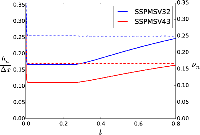
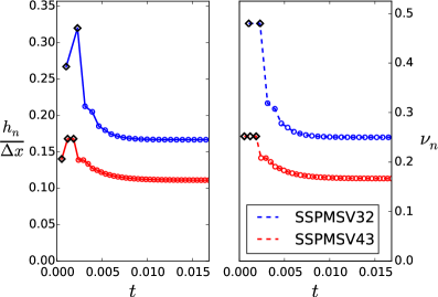
(a) Burgers’ equation

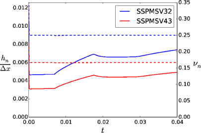
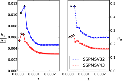
(b) Woodward–Colella blast-wave problem

Figure 1: Evolution of step size for one-dimensional Burgers’ and Euler equations with second- and third-order linear multistep methods (solid lines). The dashed curves indicate the CFL number for each method. Figures on the right show a close-up view of the step size and CFL number at early times. The black marks indicate the starting Runge–Kutta method’s step sizes.

6.7 Two-dimensional shallow-water flow

Consider the two-dimensional shallow-water equations

$$h_{t}+(hu)_{x}+(hv)_{y} =0$$

$$(hu)_{t}+(hu^{2}+\frac{1}{2}gh^{2})_{x}+(huv)_{y} =0$$

$$(hv)_{t}+(huv)_{x}+(hv^{2}+\frac{1}{2}gh^{2})_{y} =0,$$

where $h$ is the depth, $(u,v)$ the velocity vector and $hu$, $hv$ the momenta in each direction. The gravitational constant $g$ is equal to unity. The domain is a square $[-2.5,2.5]\times[-2.5,2.5]$ with $250$ grid cells in each direction. The initial condition consists of an uplifted, inward-flowing cylindrically symmetric perturbation given by

$$h(x,y,0)=1+g(x,y),\quad u(x,y,0)=-xg(x,y)\quad\text{ and }\quad v(x,y,0)=-yg(x,y),$$

where $g(x,y):=e^{-10\left(\sqrt{x^{2}+y^{2}}-1\right)^{2}}$. We apply reflecting boundary conditions at the top and right boundary, whereas the bottom and left boundaries are outflow. The wave is initially directed towards the center of the domain, and a large peak forms as it converges there, before subsequently expanding outward. We compute the solution up to time $t=2.5$, after the solution has been reflected from the top and right boundaries. Figure 2a shows how the step size varies in time. It decreases as the initial profile propagates towards the center of the domain since the maximum wave speed increases. As the solution expands outwards, higher step sizes are allowed. Note that at time $t\approx 2$ the wave hits the boundaries, so a small decrease in the allowed step size is observed. Again, the dashed curves indicate the variation of the CFL number. Now we have the ratio $s\approx 0.62$ for both second- and third-order methods.

6.8 Shock-bubble interaction

Finally, we consider the Euler equations of compressible fluid dynamics in cylindrical coordinates. Originally, the problem is three-dimensional but can been reduced to two dimensions by using cylindrical symmetry. The resulting system of equations is

$$\rho_{t}+(\rho u)_{z}+(\rho v)_{r} =-\frac{\rho v}{r}$$

$$(\rho u)_{t}+(\rho u^{2}+p)_{z}+(\rho uv)_{r} =-\frac{\rho uv}{r}$$

$$(\rho v)_{t}+(\rho uv)_{z}+(\rho v^{2}+p)_{r} =-\frac{\rho v^{2}}{r}$$

$$(\rho E)_{t}+(u(\rho E+p))_{z}+(v(\rho E+p))_{r} =-\frac{(\rho E+p)v}{r}.$$

Here, $\rho$ is the density, $p$ is the pressure, $E$ is the total energy, while $u$ and $v$ are the $z$- and $r$-components of the velocity. The $z$- and $r$-axis are parallel and perpendicular, respectively, to the axis of symmetry. The problem involves a planar shock wave traveling in the $z$-direction that impacts a spherical low-density bubble. The initial conditions are taken from [Ket+12]. We consider a cylindrical domain $[0,2]\times[0,0.5]$ using a $640\times 160$ grid and impose reflecting boundary conditions at the bottom of the domain and outflow conditions at the top and right boundaries.

Since the fluid is a polytropic ideal gas, the internal energy $e$ is proportional to the temperature. Initially the bubble is at rest, hence there is no difference in pressure between the bubble and the surrounding air. Therefore, the temperature inside the bubble is high resulting in large sound speed $c=\sqrt{\gamma(\gamma-1)e}$, where $\gamma=1.4$. Consequently, this results in reduced step sizes right after the shock wave hits the bubble at $t\approx 0.05$, as shown in Figure 2b. The efficiency ratio $s$ is about $0.82$.

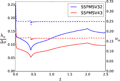
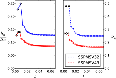
(a) Shallow-water equations

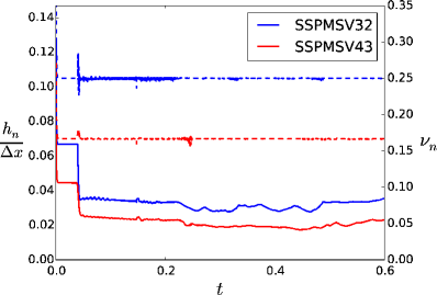
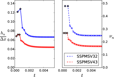
(b) Shock-bubble interaction problem

Figure 2: Evolution of step size for two-dimensional shallow-water and Euler equations with second- and third-order linear multistep methods (solid lines). The dashed curves indicate the CFL number for each method. Figures on the right show a close-up view of the step size and CFL number at early times. The black marks indicate the starting Runge–Kutta method’s step sizes.

7 Conclusions

The methods presented in this paper are the first adaptive multistep methods that provably preserve any convex monotonicity property satisfied under explicit Euler integration. We have provided a step-size selection algorithm—yielding an optimal step-size sequence $h_{n}$—that strictly enforces this property while ensuring that the step size is bounded away from zero. The methods are proved to converge at the expected rate for any ODE system satisfying the forward Euler condition.

As suggested by Theorems 6 and  7, for all tests the CFL number remains close to $\frac{k-p}{k-1}\nu_{\textup{FE}}$, where $k$ and $p$ are the steps and order of the method, respectively. The numerical results verify that the step size is approximately inversely proportional to the maximum wave speed and the proposed step-size strategy successfully chooses step sizes closely related to the maximum allowed CFL number. In practice, we expect that conditions (34) and (40), which were introduced only as technical assumptions for some of our theoretical results, could usually be omitted without impacting the solution.

The methods presented herein are of orders two and three. We have proved the existence of methods of arbitrary order. However, the optimal methods for orders at least 3 seem to have a complicated structure. It would be useful to develop adaptive (and possibly suboptimal) multistep SSP methods of order higher than three having a simple structure.

8 The proofs of the theorems in Section 3

We present three lemmas, Lemma 2 below, Lemma 3 in Section 8.1 and Lemma 4 in Section 8.2, that are used in the proofs of Theorems 2-5 in Sections 8.1-8.4. Lemmas 2-4 are straightforward generalizations of the corresponding results of [NK16] for variable step-size formulae, hence their proofs are omitted here.

Lemma 2.

Let $r\geq 0$ be arbitrary and let $p$ and $n\geq k$ be arbitrary positive integers. Suppose that some time-step ratios $\omega_{j,n}>0$ are given. Then the following two statements are equivalent.

1. For all formulae with $k$ steps and order of accuracy $p$ we have ${\mathcal{C}}_{n}(\omega,\delta,\beta)\leq r$.

2. There exists a non-zero real univariate polynomial $q_{n}$ of degree at most $p$, that satisfies the conditions

   $$q_{n}(\Omega_{j,n}) \geq 0 \text{ for all }0\leq j\leq k-1,$$ (45a)

   $$q_{n}^{\prime}(\Omega_{j,n})+rq_{n}(\Omega_{j,n}) \geq 0 \text{ for all }0\leq j\leq k-1,$$ (45b)

   $$q_{n}(\Omega_{k,n}) =0.$$ (45c)

Furthermore, if statement $(i)$ holds, then the polynomial $q_{n}$ can be chosen to satisfy the following conditions.

1. The degree of $q_{n}$ is exactly $p$.

2. The real parts of all roots of $q_{n}$ except for $\Omega_{k,n}$ lie in the interval $[\Omega_{0,n},\Omega_{k-1,n}]$.

3. The set of all real roots of $q_{n}$ is a subset of $\{\Omega_{0,n},\Omega_{1,n},\ldots,\Omega_{k,n}\}$.

4. For even $p$, $\Omega_{0,n}$ is a root of $q_{n}$ with odd multiplicity. For odd $p$, if $\Omega_{0,n}$ is a root of $q_{n}$, then its multiplicity is even.

5. The multiplicity of the root $\Omega_{k,n}$ is one. For $1\leq j\leq k-1$, if $\Omega_{j,n}$ is a root of $q_{n}$, then its multiplicity is 2.

6. The polynomial $q_{n}$ is non-negative on the interval $[\Omega_{0,n},\Omega_{k,n}]$.

The following observation will be useful in the proofs. If $q_{n}(\Omega_{j,n})=0$, then the inequality (45b) for this index $j$ simplifies to $q_{n}^{\prime}(\Omega_{j,n})\geq 0$. Otherwise, if $q_{n}(\Omega_{j,n})\neq 0$, then the inequality (45b) for this index $j$ can be written by using the logarithmic derivative of $q_{n}$ as

$$\frac{q_{n}^{\prime}(\Omega_{j,n})}{q_{n}(\Omega_{j,n})}=\sum\limits_{\ell=1}^{p}\frac{1}{\Omega_{j,n}-\lambda_{\ell,n}}\geq-r,$$

where the $\lambda_{\ell,n}$ numbers are the complex (including real) roots of $q_{n}$, and $q_{n}$ has been chosen such that its degree is exactly $p$.

8.1 The proof of Theorem 2

The following lemma will be used in the second step of the proof of Theorem 2.

Lemma 3.

Let $r>0$ be arbitrary and let $p$ and $n\geq k$ be arbitrary positive integers. Suppose that some time-step ratios $\omega_{j,n}>0$ are given. Then exactly one of the following statements is true.

1. There is a formula with $k$ steps, order of accuracy $p$ and ${\mathcal{C}}_{n}(\omega,\delta,\beta)\geq r$.

2. There is a real univariate polynomial $q_{n}$ of degree at most $p$, that satisfies the conditions (45a), (45b) and

   $$q_{n}(\Omega_{k,n})<0.$$ (46)

The proof of Theorem 2.

Step 1. To prove the bound (18), we first consider the $k\geq 2$ case, and let $q_{n}$ denote the polynomial

$$q_{n}(x):=x^{p-1}(\Omega_{k,n}-x).$$ (47)

$\bullet$ If $\Omega_{k,n}>p$, this $q_{n}$ satisfies conditions (45) with $r:=\left({\Omega_{k,n}-p}\right)/\left({\Omega_{k,n}-1}\right)$, since for each $1\leq j\leq k-1$ we have

$$\frac{q_{n}^{\prime}(\Omega_{j,n})}{q_{n}(\Omega_{j,n})}=\frac{p-1}{\Omega_{j,n}}-\frac{1}{\Omega_{k,n}-\Omega_{j,n}}\geq\frac{p-1}{\Omega_{k-1,n}}-\frac{1}{\Omega_{k,n}-\Omega_{k-1,n}}=-\frac{\Omega_{k,n}-p}{\Omega_{k,n}-1},$$

and $q_{n}^{\prime}(\Omega_{0,n})\equiv q_{n}^{\prime}(0)\geq 0$.

$\bullet$ If $\Omega_{k,n}\leq p$, the conditions (45) hold with $r:=0$, because for $x\in[\Omega_{0,n},\Omega_{k-1,n}]\equiv[0,\Omega_{k,n}-1]$ we have

$$q_{n}^{\prime}(x)\geq x^{p-2}\left((p-1)\Omega_{k,n}-p\left(\Omega_{k,n}-1\right)\right)=x^{p-2}\left(p-\Omega_{k,n}\right)\geq 0.$$

For $k=1$, the same $q_{n}$ as in (47) satisfies (45) with $r:=0$ and $\Omega_{k,n}=1$. Then, in each case, (18) is an immediate consequence of Lemma 2.

Step 2. Suppose now

$$\exists\text{ a }k\text{-step explicit linear multistep formula of order }p\geq 2\text{ with }{\mathcal{C}}_{n}(\omega,\delta,\beta)>0.$$ (48)

We prove that there is a $k$-step formula of order $p$ whose SSP coefficient is equal to the optimal one.

Let us set ${\cal{H}}:=\{r>0:\text{the statement }(ii)\text{ of Lemma \ref{lem:farkas}\, holds}\}$. Step 1 implies that the largest possible ${\mathcal{C}}_{n}(\omega,\delta,\beta)$ for all $k$-step formulae of order $p$ and having the given time-step ratios $\omega_{j}$ is finite. So ${\cal{H}}\neq\varnothing$ by Lemma 3. We also see that ${\cal{H}}$ is an infinite interval, because if a polynomial $q_{n}$ satisfies the conditions (45a), (45b) with some $r:=\rho>0$, and (46), then it satisfies the same conditions with any $r\in(\rho,+\infty)$. Thus, with a suitable $r^{*}\geq 0$, we have $(r^{*},+\infty)\subseteq{\cal{H}}\subseteq[r^{*},+\infty)$. Clearly, $r^{*}>0$ due to assumption (48) and Lemma 3. We claim that $r^{*}\notin{\cal{H}}$.

Suppose to the contrary that $r^{*}\in{\cal{H}}$. Then there is a polynomial $q_{n}$ satisfying the conditions (45a), (45b) with $r:=r^{*}$, and (46). Now we define $\widetilde{q}_{n}:=q_{n}+\left|q_{n}(\Omega_{k,n})\right|/2$. One easily checks that this $\widetilde{q}_{n}$ polynomial satisfies the same set of conditions with

$$r:=\left(\frac{1+\max\limits_{0\leq j\leq k-1}q_{n}(\Omega_{j,n})}{1+{\left|q_{n}(\Omega_{k,n})\right|}/{2}+\max\limits_{0\leq j\leq k-1}q_{n}(\Omega_{j,n})}\right)\cdot r^{*}\in(0,r^{*}),$$

so we would get $(0,r^{*})\cap{\cal{H}}\neq\varnothing$, a contradiction.

Hence ${\cal{H}}=(r^{*},+\infty)$. Therefore, in view of Lemma 3, $r^{*}$ is the optimal SSP coefficient and there exists an optimal method with ${\mathcal{C}}_{n}(\omega,\delta,\beta)=r^{*}$. ∎

8.2 The proof of Theorem 3

In the following we apply the usual terminology and say that an inequality constraint is binding if the inequality holds with equality. The lemma below is used in the proofs of Theorems 3 and 4.

Lemma 4.

Let $n\geq k$ be arbitrary positive integers and $p\geq 2$. Suppose that the time-step ratios $\omega_{j,n}>0$ are given, and that there exists an explicit linear multistep formula with $k$ steps, order of accuracy $p$, and ${\mathcal{C}}_{n}>0$. Let $\delta_{j,n}$ and $\beta_{j,n}$ denote the coefficients of a formula with the largest SSP coefficient ${\mathcal{C}}_{n}(\omega_{n},\delta_{n},\beta_{n})\in(0,+\infty)$. Let $q_{n}$ be a polynomial that satisfies all the conditions of Lemma 2 with $r:={\mathcal{C}}_{n}(\omega_{n},\delta_{n},\beta_{n})$. Then the following statements hold.

1. If $\delta_{j,n}\neq 0$ for some $0\leq j\leq k-1$, then $q_{n}(\Omega_{j,n})=0$.

2. If $\beta_{j,n}\neq 0$ for some $0\leq j\leq k-1$, then $q_{n}^{\prime}(\Omega_{j,n})+rq_{n}(\Omega_{j,n})=0$.

3. This $q_{n}$ can be chosen so that the total number of binding inequalities in (45a)-(45b) is at least $p$.

The proof of Theorem 3.

The necessity of the condition $\Omega_{k,n}>2$ for the existence of a second-order formula with positive SSP coefficient is an immediate consequence of Theorem 2. On the other hand, we easily see that, up to a positive multiplicative constant, $q_{n}(x)=x(\Omega_{k,n}-x)$ is the unique polynomial satisfying (45a), (45c), and Properties 1 and 4 of Lemma 2. If $\Omega_{k,n}>2$, then $q_{n}$ does not satisfy (45b) with $r:=0$ for $j=k-1$, therefore there exists a formula with ${\mathcal{C}}_{n}>0$ due to Lemma 2. Thus the condition $\Omega_{k,n}>2$ is also sufficient.

From now on we assume $\Omega_{k,n}>2$, and that a formula with the optimal SSP coefficient ${\mathcal{C}}_{n}(\omega_{n},\delta_{n},\beta_{n})$ is considered. From the above form of $q_{n}$ we see that $q_{n}(\Omega_{j,n})=0$ ($0\leq j\leq k-1$) holds only for $j=0$, so the statement $(iii)$ of Lemma 4 guarantees that at least one of the inequalities in (45b) is binding with $r:={\mathcal{C}}_{n}(\omega_{n},\delta_{n},\beta_{n})$. Since $q_{n}^{\prime}(\Omega_{0,n})+rq_{n}(\Omega_{0,n})=\Omega_{k,n}>0$ and for all $1\leq j\leq k-2$ we have

$$\frac{q_{n}^{\prime}(\Omega_{j,n})}{q_{n}(\Omega_{j,n})}=\frac{1}{\Omega_{j,n}}-\frac{1}{\Omega_{k,n}-\Omega_{j,n}}>\frac{1}{\Omega_{k-1,n}}-\frac{1}{\Omega_{k,n}-\Omega_{k-1,n}}=-\frac{\Omega_{k-1,n}-1}{\Omega_{k-1,n}},$$

the unique binding inequality in (45b) must be the one corresponding to the index $j=k-1$. But $q_{n}^{\prime}(\Omega_{k-1,n})+rq_{n}(\Omega_{k-1,n})=0$ implies $r=\left({\Omega_{k,n}-2}\right)/\left({\Omega_{k,n}-1}\right)$.

Finally, the statements $(i)$ and $(ii)$ of Lemma 4 guarantee that only $\delta_{0,n}$ and $\beta_{k-1,n}$ can differ from zero. Solving the conditions for order two (see (17)) then yields the unique formula stated in (19). ∎

8.3 The proof of Theorem 4

First we present a lemma that will be used in the proof of Theorem 4. Moreover, Statement 2 of the lemma proves our claim about the unique real root of the polynomial $P_{k+j}$ in (22) under assumption (24), hence guaranteeing that the quantity $r_{k+j}$ in (25) has a proper definition. The $\Delta_{j}$ quantities defined in (23) clearly satisfy the condition $1<\Delta_{j+1}<\Delta_{j}$ below.

Lemma 5.

Let some $1<\Delta_{j+1}<\Delta_{j}$ numbers be given, and for any $\rho\in\mathbb{R}$ let

$$A_{j}(\rho):=\begin{pmatrix}\rho-2&\rho-1&\rho-3\\ \rho\Delta_{j}^{2}-2\Delta_{j}&\rho\Delta_{j}-1&\rho\Delta_{j}^{3}-3\Delta_{j}^{2}\\ \rho\Delta_{j+1}^{2}-2\Delta_{j+1}&\rho\Delta_{j+1}-1&\rho\Delta_{j+1}^{3}-3\Delta_{j+1}^{2}\end{pmatrix}\begin{matrix}\vphantom{}\\ \vphantom{}\\ \vphantom{}.\end{matrix}$$ (49)

Then the following statements hold.

1. Every real root of the polynomial $P_{k+j}$ (appearing in (22)) is positive.

2. Under condition (24), $P_{k+j}$ has a unique real root.

3. If

   $$\exists(r,a,b)\in\mathbb{R}^{3}\text{ satisfying }A_{j}(r)\cdot(a,b,1)^{\top}=0\text{ and }a^{2}-4b<0,$$ (50)

   then

   $$\eqref{22cond}\quad\text{and}\quad P_{k+j}(r)=0$$ (51)

   hold.

4. If (51) holds with some $r\in\mathbb{R}$, then (50) is true, and the triplet $(r,a,b)\in\mathbb{R}^{3}$ is unique.

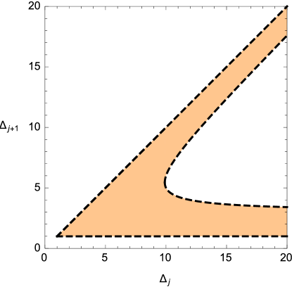
Figure 3: The set defined by (24).

Proof.

Throughout the proof we always assume $1<\Delta_{j+1}<\Delta_{j}$ and $r\in\mathbb{R}$. First we define some auxiliary polynomials—their dependence on $\Delta_{j+1}$ is suppressed for brevity.

$\widetilde{P}_{1}(r):=(r^{2}-r)\Delta_{j+1}-r+2$,

$\widetilde{P}_{2}(r):=(r^{2}-2r)\Delta_{j+1}-2r+6$,

$\widetilde{P}_{3}(r):=(r^{2}-r^{3})\Delta_{j+1}^{2}+2(r^{2}-2r)\Delta_{j+1}-2r+6$,

$\widetilde{P}_{4}(r):=r^{2}\left(r^{2}-4r+2\right)\Delta_{j+1}^{2}-4r\left(r^{2}-5r+3\right)\Delta_{j+1}+2\left(r^{2}-6r+6\right)$,

$\widetilde{P}_{5}(r):=\left(-\left(5+2\sqrt{6}\right)r^{3}+2\left(3+\sqrt{6}\right)r^{2}-2r\right)\Delta_{j+1}+\left(5+2\sqrt{6}\right)r^{2}-4\left(3+\sqrt{6}\right)r+6$,

$\widetilde{P}_{6}(r):=(r-1)\Delta_{j+1}-r+3$,

$\widetilde{P}_{7}(r):=r^{2}\Delta_{j+1}^{2}-4r\Delta_{j+1}+6$,

$\widetilde{P}_{8}(x,a,r):=(r^{2}-r)x^{2}+(r-1)(ar+r-3)x+a(2-r)-r+3$,

$\widetilde{P}_{9}(r):=(r-r^{2})\Delta_{j+1}^{2}-\left(r^{2}-4r+3\right)\Delta_{j+1}+r-3$,

$\widetilde{P}_{10}(r):=(r^{2}-r)\Delta_{j+1}-r+3$,

$\widetilde{P}_{11}(r):=r\Delta_{j+1}^{2}-(r+3)\Delta_{j+1}+1$.

Step 1. Statement 1 follows from the fact that the coefficient of $x^{m}$ in $P_{k+j}(x)$ is positive for odd $m$ and negative for even $m$, so $P_{k+j}$ cannot have a non-positive root.

Step 2. We now prove Statement 2. Since $P_{k+j}$ is cubic, it has a real root. By taking into account Statement 1, we will show that

$$\exists r>0\ :\ \eqref{22cond},\ P_{k+j}(r)=0\ \text{ and }\ P_{k+j}^{\prime}(r)\leq 0$$ (52)

is false, implying that $P_{k+j}^{\prime}>0$ at every real root of $P_{k+j}$, which is possible only if $P_{k+j}$ has a unique real root.

If $\widetilde{P}_{1}(r)=0$, we obtain

$$(r,\Delta_{j+1})=(2-\sqrt{2},3+2\sqrt{2})$$ (53)

by using $P_{k+j}(r)=0$ also. But then one easily shows that (52) is impossible.

So we can suppose in the rest of Step 2 that $\widetilde{P}_{1}(r)\neq 0$. Then from $P_{k+j}(r)=0$ we get

$$\Delta_{j}=\widetilde{P}_{2}(r)/({r\widetilde{P}_{1}(r)}).$$ (54)

This form of $\Delta_{j}$ is substituted into (52) and we obtain

$$r>0\quad\text{and}\quad{\widetilde{P}_{3}(r)}/{\widetilde{P}_{1}(r)}>0\quad\text{and}\quad\widetilde{P}_{4}(r)/\widetilde{P}_{1}(r)\leq 0\quad\text{and}$$ (55)

$$\left({\widetilde{P}_{5}(r)}/{{\widetilde{P}_{1}(r)}}<0\quad\text{or}\quad{\widetilde{P}_{6}(r)\,\widetilde{P}_{7}(r)}/{\widetilde{P}_{1}(r)}>0\right).$$ (56)

Because all $\widetilde{P}_{j}$ polynomials ($1\leq j\leq 7$) are at most quadratic in $\Delta_{j+1}$, one can systematically reduce (55)-(56) to a system of univariate polynomial inequalities in $r$, and verify that (55)-(56) has no solution. This finishes the proof of Step 2.

Step 3. To prove Statement 3, notice first that

$$A_{j}(r)\cdot(a,b,1)^{\top}=0$$ (57)

implies

$$0=\det A_{j}(r)\equiv\left(\Delta_{j}-1\right)\left(\Delta_{j+1}-1\right)\left(\Delta_{j}-\Delta_{j+1}\right)P_{k+j}(r),$$ (58)

so we have $P_{k+j}(r)=0$. To show (24), depicted in Figure 3, we separate two cases.

If $r=1$, then we obtain $a=-2$ from the first component of (57), and $b=4\Delta_{j}-\Delta_{j}^{2}$ with

$$\Delta_{j+1}=4-\Delta_{j}\quad\text{ and }\quad 2<\Delta_{j}<3$$ (59)

from the other two components and from $1<\Delta_{j+1}<\Delta_{j}$. So (24) holds.

We can thus suppose in the rest of Step 3 that $r\neq 1$. Then from (57) we get

$$b=\frac{(2-r)a-r+3}{r-1}$$ (60)

and

$$\widetilde{P}_{8}(\Delta_{j},a,r)=0=\widetilde{P}_{8}(\Delta_{j+1},a,r).$$ (61)

We again separate two cases.

If $\widetilde{P}_{1}(r)=0$, then by using (61) and $1<\Delta_{j+1}<\Delta_{j}$ we obtain

$$r=2-\sqrt{2},\ \Delta_{j}>\Delta_{j+1}=3+2\sqrt{2}\quad\text{and}\quad a=-\left(\Delta_{j}+1+{1}/{\sqrt{2}}\right).$$ (62)

But it is easy to check that (62), the inequality $a^{2}-4b<0$ from (50), and the negation of (24) cannot hold simultaneously. So (24) is proved in this case.

Therefore, in the rest of Step 3, we can suppose that $\widetilde{P}_{1}(r)\neq 0$. Then $a$ is expressed from $\widetilde{P}_{8}(\Delta_{j+1},a,r)=0$ and we get

$$a={\widetilde{P}_{9}(r)}/{\widetilde{P}_{1}(r)}.$$ (63)

Moreover, we express $\Delta_{j}$ from $P_{k+j}(r)=0$ (shown to hold in (58)) as in (54). To finish Step 3, we will verify that

$$a^{2}-4b<0\text{ from }\eqref{lemma5up},\text{ and the negation of }\eqref{22cond}$$ (64)

cannot hold. The substitution of (63) and (54) into (64) yields

$$r>0,\quad\widetilde{P}_{6}(r)\widetilde{P}_{10}(r)\widetilde{P}_{11}(r)<0,\quad\widetilde{P}_{5}(r)/\widetilde{P}_{1}(r)\geq 0,\quad\text{and}\quad\widetilde{P}_{6}(r)\widetilde{P}_{7}(r)/\widetilde{P}_{1}(r)\leq 0.$$ (65)

Again, these $\widetilde{P}_{j}$ polynomials are at most quadratic in $\Delta_{j+1}$, so one can check that (65) has no solution.

Step 4. To prove Statement 4, we first suppose that

$$r\neq 1\quad\text{and}\quad\widetilde{P}_{1}(r)\neq 0.$$ (66)

Then we have seen in Step 3 that if $(a,b)\in\mathbb{R}^{2}$ solves (57), then $a$ and $b$ necessarily have the form (63) and (60), respectively; and the uniqueness of $r$ is guaranteed by Step 2. So, under condition (66), any triplet solving (57) is unique. On the other hand, direct substitution into (57) shows that the above $(r,a,b)$ is indeed a solution—the non-trivial component to check in (57) is the second one, which is just $\left(\Delta_{j}-1\right)\left(\Delta_{j}-\Delta_{j+1}\right)P_{k+j}(r)/\widetilde{P}_{1}(r)=0$ due to $P_{k+j}(r)=0$ from assumption (51). Finally, to finish Step 4 in the case when (66) holds, we notice that for this unique triplet $(r,a,b)$ we have $a^{2}-4b=\widetilde{P}_{6}(r)\widetilde{P}_{10}(r)\widetilde{P}_{11}(r)/(\widetilde{P}_{1}(r))^{2}$. But, with $\Delta_{j}$ expressed as in (54), one can again show that

$$\widetilde{P}_{6}(r)\widetilde{P}_{10}(r)\widetilde{P}_{11}(r)\geq 0,\quad 1<\Delta_{j+1}<\Delta_{j},\quad\text{and}\quad\eqref{22cond}\text{ from assumption }\eqref{lemma5down}$$

cannot hold. This means that $a^{2}-4b<0$ from (50) also holds.

To prove Statement 4 when $r=1$, we recall from Step 3 that in this case the only possible triplet is $(r,a,b)=(1,-2,4\Delta_{j}-\Delta_{j}^{2})$ with (59), which indeed satisfy (50).

Lastly, we consider the case when $\widetilde{P}_{1}(r)=0$. We have seen in Step 2 that this time (53) holds. Since $\Delta_{j+1}<\Delta_{j}$, we also have $3+2\sqrt{2}<\Delta_{j}$. These yield that the unique solution to (57) is

$$(r,a,b)=(2-\sqrt{2},\ -(\Delta_{j}+1+{1}/{\sqrt{2}}),\ (2+\sqrt{2})\Delta_{j}).$$

Now (24) implies $\Delta_{j}<5+{7}/{\sqrt{2}}$, so $a^{2}-4b=\Delta_{j}^{2}-3(2+\sqrt{2})\Delta_{j}+\sqrt{2}+{3}/{2}<0$, and the proof is complete. ∎

The proof of Theorem 4.

Step 1. The necessity of the condition $\Omega_{k,n}>3$ for the existence of a third-order formula with positive SSP coefficient is again an immediate consequence of Theorem 2. To see that this condition is also sufficient, suppose to the contrary that there is no third-order formula with $k$ steps, positive SSP coefficient and $\Omega_{k,n}>3$, and let us apply Lemma 2 with $r:=0$. First we show that, up to a positive multiplicative constant, $q_{n}(x)=x^{2}(\Omega_{k,n}-x)$ is the unique polynomial satisfying (45), and Properties 1–2 and 4–5 of Lemma 2. Indeed, (45a)–(45b) with $j=0$ and $r=0$, together with Properties 2 and 5 imply that $\Omega_{0,n}=0$ is a root of $q_{n}$ (otherwise the logarithmic derivative of $q_{n}$ at $0$ would be negative), and then the multiplicity of $0$ is precisely two due to Properties 1 and 4, so the desired form of $q_{n}$ follows. Now, applying (45b) with $j=k-1$ and $r=0$ to this $q_{n}$ gives $\left(3-\Omega_{k,n}\right)\left(\Omega_{k,n}-1\right)\geq 0$, contradicting to $\Omega_{k,n}>3$. This contradiction proves the sufficiency of the condition $\Omega_{k,n}>3$.

Step 2. From now on we assume $\Omega_{k,n}>3$, and that a formula with the optimal SSP coefficient $r:={\mathcal{C}}_{n}(\omega_{n},\delta_{n},\beta_{n})\in(0,+\infty)$ is considered. Let $q_{n}$ be a polynomial satisfying conditions (45), Properties 1–6 of Lemma 2, and the condition $(iii)$ of Lemma 4.

Case I. In the case when $\Omega_{k,n}$ is not the only real root of $q_{n}$, then, due to Properties 1, 3 and 5 of Lemma 2, $q_{n}$ is unique (up to a positive multiplicative constant) and takes the form $q_{n}(x)=(x-\Omega_{j_{0},n})^{2}(\Omega_{k,n}-x)$ with an appropriate index $0\leq j_{0}\leq k-1$. We notice that the only binding inequality in (45a) is the one corresponding to $j=j_{0}$, and the $j=j_{0}$ inequality in (45b) is also binding (independently of the value of $r$). On the other hand, now all roots of $q_{n}$ are real, so the logarithmic derivative of $q_{n}$ is strictly decreasing on the intervals $[\Omega_{0,n},\Omega_{j_{0},n})$ and $(\Omega_{j_{0},n},\Omega_{k-1,n}]$. Thus, by $(iii)$ of Lemma 4, (45b) contains either two or three binding inequalities, and they correspond to

• $j\in\{0,k-1\}$ for $j_{0}=0$,

• $j\in\{j_{0}-1,j_{0}\}$ or $j\in\{j_{0},k-1\}$ for $1\leq j_{0}\leq k-2$,

• $j\in\{k-2,k-1\}$ for $j_{0}=k-1$.

In Case A, (45b) is solved with $j=k-1$, and we obtain $r={(\Omega_{k,n}-3)}/{(\Omega_{k,n}-1)}$. Due to $(i)$ and $(ii)$ of Lemma 4, all formula coefficients except for possibly $\{\delta_{0,n},\beta_{0,n},\allowbreak\beta_{k-1,n}\}$ vanish.
In Case B, (45b) is solved with $j=j_{0}-1$ and $j=k-1$ to get $r={2}/{(\Omega_{j_{0},n}-\Omega_{j_{0}-1,n})}+{1}/({\Omega_{k,n}-\Omega_{j_{0}-1,n}})$ and $r={(\Omega_{k,n}-\Omega_{j_{0},n}-3)}/{(\Omega_{k,n}-\Omega_{j_{0},n}-1)}$, respectively, then the maximum is chosen. If these two expressions for $r$ are not equal, we get from $(i)$ and $(ii)$ of Lemma 4 that the number of non-zero formula coefficients is at most three; whereas if the two expressions for $r$ are equal, the number of non-zero formula coefficients is at most four.
In Case C, (45b) is solved with $j=k-2$ to yield $r={2}/{(\Omega_{k-1,n}-\Omega_{k-2,n})}+{1}/{(\Omega_{k,n}-\Omega_{k-2,n})}$. All formula coefficients except for possibly $\{\delta_{k-1,n},\beta_{k-2,n},\beta_{k-1,n}\}$ vanish.

Therefore, the optimal SSP coefficient is equal to one of the $r_{j}$ quantities ($0\leq j\leq k-1$) defined in Section 3.3, and the non-zero formula coefficients also have the form stated there.

Case II. In the case when $\Omega_{k,n}$ is the only real root of $q_{n}$, then, by taking into account (45a), and Properties 1 and 5 of Lemma 2, $q_{n}$ (up to a positive multiplicative constant) has the form

$$q_{n}(x)=(\Omega_{k,n}-x)\left((\Omega_{k,n}-x)^{2}+a(\Omega_{k,n}-x)+b\right)$$

with some coefficients $a,b\in\mathbb{R}$ satisfying the discriminant condition $a^{2}-4b<0$. Let us introduce the abbreviation $Q_{3}:=q_{n}^{\prime}+rq_{n}$.

This time there are no binding inequalities in (45a), so, due to $(iii)$ of Lemma 4, precisely three inequalities are binding in (45b)—there can be no more, since the polynomial $Q_{3}$ is cubic. Let $0\leq j_{0}<j_{1}<j_{2}\leq k-1$ denote the three indices corresponding to these binding inequalities, then $Q_{3}(\Omega_{j_{0},n})=Q_{3}(\Omega_{j_{1},n})=Q_{3}(\Omega_{j_{2},n})=0$. We observe that the leading coefficient of $Q_{3}$ is $-r<0$, and $Q_{3}(\Omega_{k,n})=-b<0$ because of $a^{2}-4b<0$. As $\Omega_{j,n}$ is strictly increasing in $j$, we get that $Q_{3}$ is positive on $(-\infty,\Omega_{j_{0},n})\cup(\Omega_{j_{1},n},\Omega_{j_{2},n})$, and negative on $(\Omega_{j_{0},n},\Omega_{j_{1},n})\cup(\Omega_{j_{2},n},+\infty)$. Hence neither $j_{1}\geq j_{0}+2$ nor $j_{2}\leq k-2$ can occur (otherwise $Q_{3}(\Omega_{j_{0}+1,n})<0$ or $Q_{3}(\Omega_{k-1,n})<0$ would contradict to (45b)). This shows that the binding inequalities in (45b) are the ones corresponding to the index set $j\in\{j_{0},j_{0}+1,k-1\}$ with an appropriate index $0\leq j_{0}\leq k-3$. The previous sentence can be rewritten as $A_{j_{0}}(r)\cdot(a,b,1)^{\top}=0$, with the matrix $A_{j_{0}}$ defined in (49). Since now $a^{2}-4b<0$ as well, so (50) is also satisfied. Hence (24) and $P_{k+j_{0}}(r)=0$ hold by Lemma 5. Due to uniqueness we see that $r=r_{k+j_{0}}$, with $r_{k+j_{0}}$ defined in (25).

Thus, the optimal SSP coefficient is equal to one of the $r_{k+j_{0}}$ quantities ($0\leq j_{0}\leq k-3$), and we get from $(ii)$ of Lemma 4 that all formula coefficients except for possibly $\{\beta_{j_{0},n},\beta_{j_{0}+1,n},\beta_{k-1,n}\}$ vanish.

Step 3. Finally, in order to conclude that the optimal SSP coefficient ${\mathcal{C}}_{n}(\omega_{n},\delta_{n},\beta_{n})$ is in fact the minimum of the $r_{j}$ expressions defined in Section 3.3, we show that ${\mathcal{C}}_{n}(\omega_{n},\delta_{n},\beta_{n})\leq r_{j}$ for any $0\leq j\leq 2k-3$.

Indeed, fix any $0\leq j_{0}\leq k-1$ and define $q_{n}(x):=(x-\Omega_{j_{0},n})^{2}(\Omega_{k,n}-x)$. The inequalities (45a) and (45c) are trivially satisfied. We verify (45b) with $r:=r_{j_{0}}$ by setting $\widetilde{Q}_{3}:=q_{n}^{\prime}+rq_{n}$ and distinguishing three cases.

• If $j_{0}=0$, then one checks that the three roots of $\widetilde{Q}_{3}$ are found at $\{x_{1},0,\Omega_{k-1,n}\}$ with $x_{1}=-{2\Omega_{k,n}}/\left({\Omega_{k,n}-3}\right)<0$.

• If $1\leq j_{0}\leq k-2$ and

  $$\frac{\Omega_{k,n}-\Omega_{j_{0},n}-3}{\Omega_{k,n}-\Omega_{j_{0},n}-1}<\frac{2}{\omega_{j_{0},n}}+\frac{1}{\Omega_{k,n}-\Omega_{j_{0}-1,n}},$$ (67)

  then the three roots of $\widetilde{Q}_{3}$ are found at $\{\Omega_{j_{0}-1,n},\Omega_{j_{0},n},x_{3}\}$ with $\Omega_{k-1,n}<x_{3}<\Omega_{k,n}$. If we have “$>$” in (67), then the three roots of $\widetilde{Q}_{3}$ are found at $\{x_{1},\Omega_{j_{0},n},\Omega_{k-1,n}\}$ with $\Omega_{j_{0}-1,n}<x_{1}<\Omega_{j_{0},n}$. Finally, if there is “$=$” in (67), then the roots of $\widetilde{Q}_{3}$ are found at $\{\Omega_{j_{0}-1,n},\Omega_{j_{0},n},\Omega_{k-1,n}\}$.

• If $j_{0}=k-1$, then the three roots of $\widetilde{Q}_{3}$ are found at $\{\Omega_{k-2,n},\Omega_{k-1,n},x_{3}\}$ with $\Omega_{k-1,n}<x_{3}<\Omega_{k,n}$.

These, combined with the fact that the leading coefficient of $\widetilde{Q}_{3}$ is negative, mean that all inequalities in (45) are satisfied. Thus, in view of Lemma 2, ${\mathcal{C}}_{n}\leq r_{j_{0}}$.

Now fix an arbitrary index $0\leq j_{0}\leq k-3$. The inequality ${\mathcal{C}}_{n}\leq r_{k+j_{0}}$ is trivial if $r_{k+j_{0}}=+\infty$. Otherwise, if $r_{k+j_{0}}<+\infty$ in (25), then, by definition, (24) and $P_{k+j_{0}}(r_{k+j_{0}})=0$ hold. So due to Lemma 5, (50) holds with $r:=r_{k+j_{0}}$ and $j:=j_{0}$. By defining

$$q_{n}(x):=(\Omega_{k,n}-x)\left((\Omega_{k,n}-x)^{2}+a(\Omega_{k,n}-x)+b\right)$$

and with $a$ and $b$ given by (50), we see that (45a) and (45c) are true because of $a^{2}-4b<0$. On the other hand, the $A_{j_{0}}(r)\cdot(a,b,1)^{\top}=0$ relation in (50) expresses the fact that the inequalities corresponding to $j\in\{j_{0},j_{0}+1,k-1\}$ are binding in (45b). So, just as in Case II in Step 2, we see that $q_{n}^{\prime}+rq_{n}$ is positive on $(-\infty,\Omega_{j_{0},n})\cup(\Omega_{j_{0}+1,n},\Omega_{k-1,n})$, and negative on $(\Omega_{j_{0},n},\Omega_{j_{0}+1,n})\cup(\Omega_{k-1,n},+\infty)$. Thus all inequalities in (45b) hold. This means that $q_{n}$ satisfies conditions (45) with this $r$ value, so, in view of Lemma 2, ${\mathcal{C}}_{n}\leq r_{k+j_{0}}$. The proof of the theorem is complete. ∎

8.4 The proof of Theorem 5

Proof.

We follow the ideas of the proof given in [NK16] for the fixed-step-size case.

Suppose to the contrary that $p$, $k$ and $\omega_{j,n}$ ($1\leq j\leq k$) satisfy the conditions of the theorem for some $n\geq k$ and $K_{1},K_{2}\geq 1$, but for all formulae with $k$ steps and order of accuracy $p$, we have ${\mathcal{C}}_{n}(\omega,\delta,\beta)=0$. Then by Lemma 2, there exists a non-zero real polynomial $q_{n}$ that satisfies the conditions (45a)–(45c) with $r=0$, moreover $q_{n}\geq 0$ on $[0,\Omega_{k,n}]$ and $\deg q_{n}=p$ (Properties 1 and 6 of Lemma 2).

First we define $A:=\max_{x\in[0,\Omega_{k,n}]}q_{n}(x)$ and $b:=\max_{x\in[0,\Omega_{k,n}]}|q_{n}^{\prime}(x)|$ and we introduce the polynomial $P(x):=q_{n}\left(\frac{x+1}{2}\cdot\Omega_{k,n}\right)-\frac{A}{2}.$ Then the Markov brothers’ inequality (see, e.g., [NK16]) for the first derivative implies that

$$\max_{x\in[-1,1]}|P^{\prime}(x)|\leq p^{2}\cdot\max_{x\in[-1,1]}|P(x)|,$$

that is, $b\frac{\Omega_{k,n}}{2}\leq p^{2}\frac{A}{2}$. On the other hand, summing the lower estimates in (32) we get $\frac{k}{K_{1}}\leq\Omega_{k,n}$, implying $\frac{b}{2}\cdot\frac{k}{K_{1}}\leq\frac{b}{2}{\Omega_{k,n}}$. Thus

$${bk}/{K_{1}}\leq p^{2}A.$$ (68)

Now, because of $q_{n}(\Omega_{k,n})=0$, the Newton–Leibniz formula and elementary estimates yield that

$$A\leq\int_{0}^{\Omega_{k,n}}\max(0,-q_{n}^{\prime}(t))dt.$$ (69)

Here we notice that the polynomial $q_{n}^{\prime}$ is of degree at most $p-1$, and $q_{n}^{\prime}(\Omega_{j,n})\geq 0$ for all $0\leq j\leq k-1$, so the set

$$\{j\in\mathbb{Z}\cap[0,k-1]:\exists x\in[\Omega_{j,n},\Omega_{j+1,n}]\text{ with }q_{n}^{\prime}(x)<0\}$$

has at most ${p}/{2}$ elements. Therefore—by decomposing the interval $[0,{\Omega_{k,n}}]$ as the union of the appropriate subintervals of length $\omega_{j,n}$, and applying the upper estimate in (32) and the estimate $-q_{n}^{\prime}\leq b$ at most $p/2$ times—we get that $\int_{0}^{\Omega_{k,n}}\max(0,-q_{n}^{\prime}(t))dt\leq\frac{p}{2}K_{2}b$, and hence

$$A\leq{bpK_{2}}/{2}.$$ (70)

Inequalities (68) and (70) imply that $k\leq p^{3}K_{1}K_{2}/2$, which contradicts the assumption of Theorem 5. Hence there is a formula with $k$ steps, order of accuracy $p$, and ${\mathcal{C}}_{n}(\omega,\delta,\beta)>0$. ∎

9 The proofs of the theorems in Section 4

In Section 9.1 we first prove a theorem about the convergence of some rational recursions. This Theorem 11 will then be used in Sections 9.2 and 9.3 to prove Theorems 6 and 7, respectively.

9.1 Global attractivity in a class of higher-order rational recursions

Theorem 11.

Let us fix an integer $k\geq 3$ and a real number $A>0$. Suppose that for $1\leq j\leq k-1$ the initial values $\tau_{j}\geq 0$ are given such that $\sum_{j=1}^{k-1}\tau_{j}>0$. For any $n\geq k$ we define

$$\tau_{n}:=\frac{\sum_{j=1}^{k-1}\tau_{n-j}}{A+\sum_{j=1}^{k-1}\tau_{n-j}}.$$ (71)

Then

$$\lim_{n\to+\infty}\tau_{n}=\left\{\begin{aligned} &0,&\text{ if }\quad&k-1\leq A,\\ &\frac{k-1-A}{k-1},&\text{ if }\quad&0<A<k-1.\end{aligned}\right.$$

To prove Theorem 11, we will apply the following lemma.

Lemma 6 (Theorem A.0.1 in [KL02]).

Suppose that $a\leq b$ are given real numbers, $k\geq 3$ is a fixed integer, and the numbers $x_{j}$ are chosen such that $x_{j}\in[a,b]$ for $1\leq j\leq k-1$. Assume further that

1. $f\colon[a,b]^{k-1}\to[a,b]$ is continuous,

2. $f$ is non-decreasing in each of its arguments,

3. there is a unique $\overline{x}\in[a,b]$ such that $f(\overline{x},\overline{x},\ldots,\overline{x})=\overline{x}$,

4. and the sequence $x_{n}$ is defined for $n\geq k$ as

   $$x_{n}:=f(x_{n-1},x_{n-2},\ldots,x_{n-(k-1)}).$$

Then $\lim_{n\to+\infty}x_{n}=\overline{x}$.

The straightforward proof of Lemma 6 is found in [KL02], see their Theorem 1.4.8 (for $k=3$), Theorem A.0.1 (for $k=4$) or Theorem A.0.9 (for general $k$)—the idea of the proof is the same in the easiest case when $f$ is non-decreasing in each of its arguments. Notice that in [KL02, Theorem 1.4.8] one should have “The equation $f(x,x)=x$ has a unique solution in $[a,b]$” instead of “…  a unique positive solution”. Now we give the proof of Theorem 11.

The proof of Theorem 11.

For some $a\leq b$ (to be specified soon) we set

$$f(z_{1},z_{2},\ldots,z_{k-1}):=\frac{\sum_{j=1}^{k-1}z_{j}}{A+\sum_{j=1}^{k-1}z_{j}}$$ (72)

with $z_{j}\in[a,b]$ ($j=1,2,\ldots,k-1$). Then

$$(\partial_{j}f)(z_{1},z_{2},\ldots,z_{k-1})=\frac{A}{\left(A+\sum_{j=1}^{k-1}z_{j}\right)^{2}}>0,$$ (73)

hence $f$ is non-decreasing in each of its arguments (and trivially continuous). Notice that due to (71) we have $\tau_{n}\in(0,1)$ for any $n\geq k$, so by shifting the indices we can assume that $\tau_{j}\in(0,1)$ for $1\leq j\leq k-1$, and $\tau_{n}=f(\tau_{n-1},\tau_{n-2},\ldots,\tau_{n-(k-1)})$ for $n\geq k$. We distinguish two cases.

1. The case $k-1\leq A$. Then $f$ maps $[a,b]^{k-1}$ to $[a,b]$ with $a:=0$ and $b:=1$. Now for any $\overline{x}\in[0,1]$ we have

   $$\overline{x}-f(\overline{x},\overline{x},\ldots,\overline{x})\equiv\frac{\overline{x}[A-(k-1)+(k-1)\overline{x}]}{A+(k-1)\overline{x}}=0$$ (74)

   precisely if $\overline{x}=0$, so Lemma 6 yields $\lim_{n\to+\infty}\tau_{n}=0$.

2. The case $0<A<k-1$. We set $\tau^{*}:=\min_{1\leq j\leq k-1}\tau_{j}$. Then $\tau^{*}>0$ and $\tau_{j}\in[\tau^{*},1]$ for $1\leq j\leq k-1$.

   1. The case $\tau^{*}\geq\frac{k-1-A}{k-1}$. We choose $a:=\frac{k-1-A}{k-1}<1=:b$, and notice that $f(a,a,\ldots,a)=a$ and $f(b,b,\ldots,b)<b$. By also using the non-decreasing property of $f$ in each of its arguments we obtain that $f$ maps $[a,b]^{k-1}$ to $[a,b]$. Now for any $\overline{x}\in[a,b]$ the equality (74) holds if and only if $\overline{x}=a$, so Lemma 6 yields $\lim_{n\to+\infty}\tau_{n}=\frac{k-1-A}{k-1}$.

   2. The case $0<\tau^{*}<\frac{k-1-A}{k-1}$. This time we choose $a:=\tau^{*}<1=:b$. Since now

      $$a<f(a,a,\ldots,a)\Longleftrightarrow\tau^{*}<f(\tau^{*},\tau^{*},\ldots,\tau^{*})\Longleftrightarrow\tau^{*}<\frac{k-1-A}{k-1},$$

      we have just as before that $f$ maps $[a,b]^{k-1}$ to $[a,b]$. For any $\overline{x}\in[a,b]$ we have (74) precisely if $\overline{x}=\frac{k-1-A}{k-1}$, therefore we can use Lemma 6 again to get $\lim_{n\to+\infty}\tau_{n}=\frac{k-1-A}{k-1}$.

∎

Example 1.

The sequence $(\tau_{n})_{n\geq 1}$ defined by (71) can have long, non-monotonic starting slices. Consider, for example, the case $k=4$ with

$$\tau_{1}:=1,\quad\tau_{2}:=\frac{1}{200},\quad\tau_{3}:=\frac{95638788642}{100000000000},$$

and

$$\tau_{n}:=\frac{\tau_{n-1}+\tau_{n-2}+\tau_{n-3}}{1+\tau_{n-1}+\tau_{n-2}+\tau_{n-3}}\quad\quad\text{for }n\geq 4.$$

Then the consecutive monotone non-increasing subsequences of $\tau_{n}$ for $1\leq n\leq 1000$ has lengths

$$(2,3,2,1,2,1,2,1,2,1,2,3,3,3,3,2,1,2,1,2,1,2,1,2,3,3,3,3,2,1,2,1,2,1,2,3,3,3,3,3,917).$$

9.2 The proof of Theorem 6

Proof.

We prove the theorem for $k=3$ first. We define two sequences

$$h_{n}^{-}:=\frac{h_{n-2}^{-}+h_{n-1}^{-}}{h_{n-2}^{-}+h_{n-1}^{-}+\mu^{-}}\cdot\mu^{-},\quad h_{n}^{+}:=\frac{h_{n-2}^{+}+h_{n-1}^{+}}{h_{n-2}^{+}+h_{n-1}^{+}+\mu^{+}}\cdot\mu^{+},\quad h_{1}^{\pm}:=h_{1},\ h_{2}^{\pm}:=h_{2},$$ (75)

and their scaled counterparts $\tau_{n}^{-}:=h_{n}^{-}/\mu^{-}$, $\tau_{n}^{+}:=h_{n}^{+}/\mu^{+}$ ($n\geq 1$). Then $\tau_{n}^{-}$ and $\tau_{n}^{+}$ satisfy

$$\tau_{n}^{-}=\frac{\tau_{n-2}^{-}+\tau_{n-1}^{-}}{\tau_{n-2}^{-}+\tau_{n-1}^{-}+1},\quad\tau_{n}^{+}=\frac{\tau_{n-2}^{+}+\tau_{n-1}^{+}}{\tau_{n-2}^{+}+\tau_{n-1}^{+}+1},\quad\tau_{1}^{\pm}>0,\ \tau_{2}^{\pm}>0.$$

By applying Theorem 11 with $k=3$ and $A=1$ we see that $\tau_{n}^{-}\to{1}/{2}$ hence $h_{n}^{-}\to{\mu^{-}}/{2}$ as $n\to+\infty$. Similarly, we get $h_{n}^{+}\to{\mu^{+}}/{2}$. We now define

$$(0,+\infty)^{3}\ni(a,x,y)\mapsto\widetilde{f}(a,x,y):=a\cdot\frac{x+y}{a+x+y}$$ (76)

(cf. (72)). It is elementary to see that for any $(a,x,y)\in(0,+\infty)^{3}$ we have

$$\partial_{1}\widetilde{f}(a,x,y)=\frac{(x+y)^{2}}{(a+x+y)^{2}}>0,\quad\partial_{2}\widetilde{f}(a,x,y)=\partial_{3}\widetilde{f}(a,x,y)=\frac{a^{2}}{(a+x+y)^{2}}>0$$ (77)

(cf. (73), and notice that the function $a\mapsto\widetilde{f}(a,x,y)/a$, for example, would be monotone decreasing). Clearly, for $n=1,2$ we have

$$h_{n}^{-}\leq h_{n}\leq h_{n}^{+},$$ (78)

so we can suppose that (78) has already been proved up to some $n\geq 2$. Then by repeatedly using the inequality $\mu^{-}\leq\mu_{n}\leq\mu^{+}$ (implied by the assumption (33)), (77) and (78), we obtain

$$h_{n+1}^{-}\equiv\frac{h_{n-1}^{-}+h_{n}^{-}}{h_{n-1}^{-}+h_{n}^{-}+\mu^{-}}\cdot\mu^{-}\leq\frac{h_{n-1}+h_{n}^{-}}{h_{n-1}+h_{n}^{-}+\mu^{-}}\cdot\mu^{-}\leq\frac{h_{n-1}+h_{n}}{h_{n-1}+h_{n}+\mu^{-}}\cdot\mu^{-}\leq$$

$$\frac{h_{n-1}+h_{n}}{h_{n-1}+h_{n}+\mu_{n+1}}\cdot\mu_{n+1}\equiv h_{n+1}\leq$$

$$\frac{h_{n-1}+h_{n}}{h_{n-1}+h_{n}+\mu^{+}}\cdot\mu^{+}\leq\frac{h_{n-1}+h_{n}^{+}}{h_{n-1}+h_{n}^{+}+\mu^{+}}\cdot\mu^{+}\leq\frac{h_{n-1}^{+}+h_{n}^{+}}{h_{n-1}^{+}+h_{n}^{+}+\mu^{+}}\cdot\mu^{+}\equiv h_{n+1}^{+}.$$

This shows the validity of (78) for all $n\geq 1$ by induction. By taking $\liminf$ and $\limsup$ in (78), Theorem 6 for $k=3$ is proved.

The proof of Theorem 6 in the general case requires only formal modifications of the argument given above: Theorem 11 with a general $k\geq 3$ and with $A=1$ implies that for the corresponding sequences we have $\tau_{n}^{\pm}\to\frac{k-2}{k-1}$ as $n\to+\infty$, and the corresponding function $\widetilde{f}\colon(0,+\infty)^{k}\to(0,+\infty)$ is increasing in each of its arguments. ∎

Figure 4 gives a graphical illustration of Theorem 6 for $k=3$, using a hypothetical sequence of values for $\mu_{n}$.

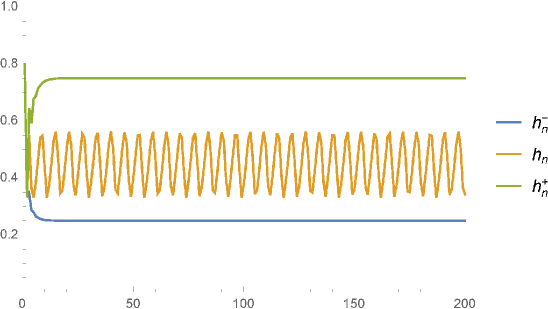
Figure 4: The first 200 terms of the sequences $h_{n}^{-}$, $h_{n}$ and $h_{n}^{+}$ with $\mu_{n}:=1+\sin(n)/2$, $\mu^{-}:=1/2$ and $\mu^{+}:=3/2$, see (35) and (75).

9.3 The proof of Theorem 7

Proof.

Step 1. Initially we suppose that some values of $\varrho>0$ and $0<\varrho_{\textup{FE}}\leq 1$ have already been chosen; we will make an actual choice for them in Step 5 so that the inductive argument given below becomes valid. First let us set $n=k$.

Step 2. We know from (40) that

$$h_{m}\leq\varrho\cdot h_{\textup{FE}}(u_{m})\quad\text{for }\ m=1,2,\ldots,n-1.$$ (79)

We will prove that

$$\sum_{j=1}^{k-1}h_{n-j}\leq\sqrt{8}\,\mu_{n}$$ (80)

and

$$h_{n}\leq\varrho\cdot h_{\textup{FE}}(u_{n}).$$ (81)

Step 3. Applying (79) and (34) repeatedly we have

$$\sum_{j=1}^{k-1}h_{n-j}\leq\varrho\cdot\sum_{j=1}^{k-1}h_{\textup{FE}}(u_{n-j})\leq\varrho\cdot\sum_{j=1}^{k-1}\frac{h_{\textup{FE}}(u_{n-1})}{(\varrho_{\textup{FE}})^{j-1}}=h_{\textup{FE}}(u_{n-1})\cdot\sum_{j=1}^{k-1}\frac{\varrho}{(\varrho_{\textup{FE}})^{j-1}}.$$ (82)

On the other hand, the definition of $\mu_{n}$ in (14), the repeated application of (34), and $0<\varrho_{\textup{FE}}\leq 1$ imply that

$$\sqrt{8}\,\mu_{n}\geq\sqrt{8}\min_{0\leq j\leq k-1}\left((\varrho_{\textup{FE}})^{j}\cdot h_{\textup{FE}}(u_{n-1})\right)=h_{\textup{FE}}(u_{n-1})\cdot\sqrt{8}\,(\varrho_{\textup{FE}})^{k-1}.$$ (83)

By comparing the right-hand sides of (82) and (83) after a division by $h_{\textup{FE}}(u_{n-1})\geq\mu^{-}>0$, we get that if $\varrho$ and $\varrho_{\textup{FE}}$ are chosen such that

$$\sum_{j=1}^{k-1}\frac{\varrho}{(\varrho_{\textup{FE}})^{j-1}}\leq\sqrt{8}\,(\varrho_{\textup{FE}})^{k-1},\quad\quad\varrho>0,\quad 0<\varrho_{\textup{FE}}\leq 1,$$ (84)

then (80) holds for this particular $n$ value.

Step 4. In order to show (81), we first notice that the function

$$(0,+\infty)^{2}\ni(z,a)\mapsto\widetilde{f}(z,a):=\frac{z}{z+2a}\cdot a$$

is increasing in each of its arguments (cf. (76)-(77)). This monotonicity property, the definition of $h_{n}$ in (39), (82), and the inequality $\mu_{n}\leq h_{\textup{FE}}(u_{n-1})$ yield that

$$h_{n}=\frac{\sum_{j=1}^{k-1}h_{n-j}}{\left(\sum_{j=1}^{k-1}h_{n-j}\right)+2\mu_{n}}\cdot\mu_{n} \leq\frac{h_{\textup{FE}}(u_{n-1})\cdot\sum_{j=1}^{k-1}\frac{\varrho}{(\varrho_{\textup{FE}})^{j-1}}}{\left(h_{\textup{FE}}(u_{n-1})\cdot\sum_{j=1}^{k-1}\frac{\varrho}{(\varrho_{\textup{FE}})^{j-1}}\right)+2h_{\textup{FE}}(u_{n-1})}\cdot h_{\textup{FE}}(u_{n-1})$$

$$=\frac{\sum_{j=1}^{k-1}\frac{\varrho}{(\varrho_{\textup{FE}})^{j-1}}}{2+\sum_{j=1}^{k-1}\frac{\varrho}{(\varrho_{\textup{FE}})^{j-1}}}\cdot h_{\textup{FE}}(u_{n-1}).$$

On the other hand, from (34) we see that $\varrho\cdot h_{\textup{FE}}(u_{n})\geq\varrho\cdot\varrho_{\textup{FE}}\cdot h_{\textup{FE}}(u_{n-1})$. Therefore if $\varrho$ and $\varrho_{\textup{FE}}$ are chosen such that

$$\frac{\sum_{j=1}^{k-1}\frac{\varrho}{(\varrho_{\textup{FE}})^{j-1}}}{2+\sum_{j=1}^{k-1}\frac{\varrho}{(\varrho_{\textup{FE}})^{j-1}}}\leq\varrho\cdot\varrho_{\textup{FE}},$$ (85)

then (81) holds for the actual $n$ value.

Step 5. So (80)-(81) will be proved as soon as we have found some $\varrho$ and $\varrho_{\textup{FE}}$ satisfying (84) and (85). Figure 5 depicts the solution set of this system of inequalities (84)-(85) in the variables $(\varrho,\varrho_{\textup{FE}})$.

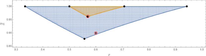
Figure 5: The solution set of the inequalities (84)-(85). In the $k=4$ case, the blue region has vertices at $(1/3,1)$, $(\sqrt{8}/3,1)$, $\approx(0.557,0.878)$. In the $k=5$ case, the orange region has vertices at $(1/2,1)$, $(1/\sqrt{2},1)$, $\approx(0.569,0.9615)$. The points corresponding to (41) have been circled.

The choice made in (41) is a simple rational pair; clearly, one could for example relax the assumption on $\varrho$ (by choosing it larger), but then condition (34) would in general become more stringent.

Step 6. According to the discussion preceding Theorem 7, on the one hand we have $\Omega_{k-1,n}>2$ hence ${\mathcal{C}}_{n}>0$. On the other hand, (80) guarantees $h_{n}={\mathcal{C}}_{n}\mu_{n}>0$ and this is the maximum value of $h_{n}$ preserving the SSP property.

Step 7. Now we repeat Steps 2-6 inductively for each $n\geq k+1$ (Step 5 is no longer needed since $(\varrho,\varrho_{\textup{FE}})$ have already been given some particular values). The range of $m$ in the induction hypothesis (79) is extended step-by-step by (81).

Step 8. Finally, to prove (42), we make use of the fact that

$$(0,+\infty)^{k}\ni(a,z_{1},z_{2},\ldots,z_{k-1})\mapsto\bar{f}(a,z_{1},z_{2},\ldots,z_{k-1}):=a\cdot\frac{\sum_{j=1}^{k-1}z_{j}}{\left(\sum_{j=1}^{k-1}z_{j}\right)+2a}$$

is increasing in each of its arguments (cf. (76)-(77)), and repeat the steps presented in Section 9.2: we define the corresponding auxiliary sequences $h_{n}^{\pm}$ and $\tau_{n}^{\pm}$ and apply Theorem 11 with $k\in\{4,5\}$ and $A=2$ to show that $\tau_{n}^{\pm}\to\frac{k-3}{k-1}$ as $n\to+\infty$. ∎

Acknowledgement

The authors would like to thank the anonymous referees for their suggestions, which have improved the presentation of the material.

References

- [Len89] Hermanus W. J. Lenferink “Contractivity-preserving explicit linear multistep methods” In Numerische Mathematik 55, 1989, pp. 213–223 DOI: 10.1007/BF01406515
- [Len91] Hermanus W. J. Lenferink “Contractivity-preserving implicit linear multistep methods” In Mathematics of Computation 56, 1991, pp. 177–199 DOI: 10.1090/S0025-5718-1991-1052098-0#sthash.JTj1dXio.dpuf
- [HRS03] Willem Hundsdorfer, Steven J. Ruuth and Raymond J. Spiteri “Monotonicity-Preserving Linear Multistep Methods” In SIAM Journal on Numerical Analysis 41, 2003, pp. 605–623 DOI: 10.1137/S0036142902406326
- [RH05] Steven J. Ruuth and Willem Hundsdorfer “High-order linear multistep methods with general monotonicity and boundedness properties” In Journal of Computational Physics 209, 2005, pp. 226–248 DOI: 10.1016/j.jcp.2005.02.029
- [HR05] Willem Hundsdorfer and Steven J. Ruuth “On monotonicity and boundedness properties of linear multistep methods” In Mathematics of Computation 75, 2005, pp. 655–672 DOI: 10.1090/S0025-5718-05-01794-1
- [Ket09] David I. Ketcheson “Computation of optimal monotonicity preserving general linear methods” In Mathematics of Computation 78.267, 2009, pp. 1497–1513 DOI: 10.1090/S0025-5718-09-02209-1
- [ZS10] Xiangxiong Zhang and Chi-Wang Shu “On maximum-principle-satisfying high order schemes for scalar conservation laws” In Journal of Computational Physics 229.9 Elsevier, 2010, pp. 3091–3120
- [GKS11] Sigal Gottlieb, David I. Ketcheson and Chi-Wang Shu “Strong Stability Preserving Runge–Kutta And Multistep Time Discretizations” World Scientific, 2011 DOI: 10.1142/7498
- [HNW93] Ernst Hairer, Syvert P. Nørsett and Gerhard Wanner “Solving ordinary differential equations I: Nonstiff Problems”, Springer Series in Computational Mathematics Springer, 1993 DOI: 10.1007/978-3-540-78862-1
- [NK16] Adrián Németh and David I. Ketcheson “Existence and optimality of strong stability preserving linear multistep methods: a duality-based approach” In preparation. Preprint available from http://arxiv.org/abs/1504.03930., 2016
- [Sch98] Alexander Schrijver “Theory of linear and integer programming” John Wiley & Sons, 1998
- [KPL13] David I. Ketcheson, Matteo Parsani and Randall J. LeVeque “High-order Wave Propagation Algorithms for Hyperbolic Systems” In SIAM Journal on Scientific Computing 35.1, 2013, pp. A351–A377 DOI: 10.1137/110830320
- [Lee77] Bram Leer “Towards the ultimate conservative difference scheme. IV. A new approach to numerical convection” In Journal of Computational Physics 23.3, 1977, pp. 276–299 DOI: 10.1016/0021-9991(77)90095-X
- [WC84] Paul Woodward and Phillip Colella “The numerical simulation of two-dimensional fluid flow with strong shocks” In Journal of Computational Physics 54.1, 1984, pp. 115–173 DOI: 10.1016/0021-9991(84)90142-6
- [Ket+12] David I. Ketcheson, Kyle T. Mandli, Aron J. Ahmadia, Amal Alghamdi, Manuel Luna, Matteo Parsani, Matthew G. Knepley and Matthew Emmett “PyClaw: accessible, extensible, scalable tools for wave propagation problems” In SIAM Journal on Scientific Computing 34.4, 2012, pp. C210–C231 DOI: 10.1137/110856976
- [KL02] Mustafa R. S. Kulenović and Gerry Ladas “Dynamics of second order rational difference equations with open problems and conjectures” Chapman & Hall/CRC, 2002 DOI: 10.1201/9781420035384