Time variation of Kepler transits induced by stellar spots —
a way to distinguish between prograde and retrograde motion.
II. Application to KOIs

Abstract

Mazeh, Holczer, and Shporer (2015) have presented an approach that can, in principle, use the derived transit timing variation (TTV) of some transiting planets observed by the Kepler mission to distinguish between prograde and retrograde motion of their orbits with respect to their parent stars’ rotation. The approach utilizes TTVs induced by spot-crossing events that occur when the planet moves across a spot on the stellar surface, looking for a correlation between the derived TTVs and the stellar brightness derivatives at the corresponding transits. This can work even in data that cannot temporally resolve the spot-crossing events themselves. Here we apply this approach to the Kepler KOIs, identifying nine systems where the photometric spot modulation is large enough and the transit timing accurate enough to allow detection of a TTV-brightness-derivatives correlation. Of those systems five show highly significant prograde motion (Kepler-17b, Kepler-71b, KOI-883.01, KOI-895.01, and KOI-1074.01), while no system displays retrograde motion, consistent with the suggestion that planets orbiting cool stars have prograde motion. All five systems have impact parameter $0.2\lesssim b\lesssim 0.5$, and all systems within that impact parameter range show significant correlation, except HAT-P-11b where the lack of a correlation follows its large stellar obliquity. Our search suffers from an observational bias against detection of high impact parameter cases, and the detected sample is extremely small. Nevertheless, our findings may suggest that stellar spots, or at least the larger ones, tend to be located at a low stellar latitude, but not along the stellar equator, similar to the Sun.

1 Introduction

Observed characteristics of exoplanet systems may contain clues to their formation process and orbital evolution history. One of the promising clues is stellar obliquity, the angle between the stellar spin and planetary orbital angular momentum, also called the spin-orbit angle. Theoretical investigations have identified processes that are expected to result in well aligned systems (e.g., Cresswell et al., 2007; Nagasawa et al., 2008; Winn et al., 2010a; Dawson, 2014), and others expected to produce misaligned orbits (e.g., Fabrycky & Tremaine, 2007; Naoz et al., 2011; Batygin, 2012). Those theories are now being put to the test using the increasing sample of host stars with measured obliquity (e.g., Triaud et al., 2010; Albrecht et al., 2012, 2013).

The growing sample has led to the detection of several possible observational trends. Fabrycky & Winn (2009) have identified early on that the sample of obliquity measurements is better explained as being composed of two different underlying distributions, one well aligned and the second isotropic, than a single distribution. Later, Winn et al. (2010a) suggested that cool stars, below $T_{\rm eff}\approx$ 6,250 K, reside in well aligned systems and that the obliquity of hotter stars cover a wider range. This was supported by a study of a larger sample by Albrecht et al. (2012) and a statistical study by Mazeh et al. (2015b). Another trend, identified by Hébrard et al. (2011), shows that planets in a retrograde orbit are less massive than a mass cut-off of about $3.5\ \rm M_{J}$, while planets above that threshold tend to be in prograde orbits. This suggests that different orbital evolution processes are at play above and below that mass threshold. More recently, Morton & Winn (2014) showed that stars hosting a multi planet system (as detected by Kepler) tend to be more well aligned than stars hosting a single planet system.

The need for a large sample of systems with a measured host star obliquity has led to the development of several methods for measuring it. Those include utilizing the Rossiter-McLaughlin (RM) effect (e.g., Gaudi & Winn, 2007), asteroseismology (e.g., Gizon & Solanki, 2003; Chaplin et al., 2013; Van Eylen et al., 2014; Lund et al., 2014), stellar rotation (e.g., Schlaufman, 2010; Hirano et al., 2012, 2014; Morton & Winn, 2014; Mazeh et al., 2015b), stellar gravity darkening (Barnes, 2009; Szabo et al., 2011; Barnes et al., 2011), the beaming effect (Photometric RM—Shporer et al. 2012; Groot 2012), and stellar activity in the form of spots (e.g., Nutzman et al., 2011; Sanchis-Ojeda et al., 2011; Sanchis-Ojeda & Winn, 2011; Désert et al., 2011; Deming et al., 2011; Sanchis-Ojeda et al., 2012, 2013).

The methods above are either statistical in nature, so no conclusions can be made about the configuration of a specific system, or require additional data—spectroscopic and/or Kepler short cadence light curves. Mazeh, Holczer, and Shporer 2015 (Hereafter Paper I) presented a new method to distinguish between prograde and retrograde motion of transiting systems for photometrically active host stars. The method utilizes spot-crossing events, where the transiting object, a planet in our case, moves across a dark spot on the surface of the host star. Unlike the approach of Nutzman et al. (2011) and Sanchis-Ojeda et al. (2011, see also ), which usually requires Kepler short cadence data, this method can use Kepler long cadence data, available for all objects observed by Kepler.

Briefly, the method presented in Paper I is based on measuring two parameters for each transit event. The first is the local stellar brightness temporal derivative at transit time, or simply the local slope, a parameter that captures the host star’s rotation phase as the spot is rotating towards or away from the center of the stellar disc. The second parameter is the transit timing variation (TTV), assumed to be induced by the spot-crossing event (e.g., Oshagh et al., 2013). Spot crossings distort the transit light curve shape, and although with long cadence data they usually cannot be fully resolved, they result in a small mid-transit time shift when fitted with a simple transit light curve model that does not account for the spot-crossing event. The TTV reflects the phase within the transit where the spot-crossing occurred. As shown in detail in Paper I, a negative (positive) correlation between the TTV and the local slope indicates a prograde (retrograde) motion, under some simplistic assumptions.

Here we present the application of the method presented in Paper I to Kepler KOIs. In Section 2 we describe our analysis and the way we identify objects with statistically significant correlation between the TTVs and local slopes. In Section 3 we discuss the transit impact parameter of the systems expected to be sensitive to TTV due to spot-crossing. In Section 4 we present the six systems for which we detect a statistically significant correlation, while in Section 5 we discuss the systems that are expected to show significant TTV due to spot-crossing although no significant correlation is detected. Section 6 presents a brief discussion and a summary.

2 Identification of KOIs with significant Correlation

As mentioned above, our method uses two parameters measured for each transit event—the TTV and the local slope of the stellar brightness at the time of the transit. Section 2.1 briefly describes the catalog of transit timing measurements we use here, and Section 2.2 describes our measurement of the local photometric slopes. In Section 2.3 we derive the correlation between the two sets of parameters for each KOI, and point to the significant detections. In Section 2.4 we discuss the sensitivity of the different systems for detecting the correlation and compare the detected systems with their sensitivity.

2.1 Transit timings

We used the transit timing catalog obtained by Holczer et al. (2015, in preparation), publicly available at: ftp://wise-ftp.tau.ac.il/pub/tauttv/TTV/ver$\_$112. The catalog includes all the KOIs listed in the NASA Exoplanet Archive, except KOIs

• labeled as false positives,

• with orbital periods longer than 300 days,

• with transit depth larger than 10 %,

• with phase folded transit signal-to-noise ratio (SNR) below 7.1,

• suspected to be binaries because of a difference in transit depth between odd and even transits,

• with folded light curve that did not display a transit with high enough significance; the p-value of the $\mathcal{F}$-test between the transit model and the no-variability model (flat line) did not yield a level of significance higher than 10^-4.

After removing all these KOIs, we are left with 2,600 systems.

The full list includes a total of 295,373 individual transits. Of those, 71,240 were rejected based on (1) an $\mathcal{F}$-test comparing the individual transit model with a flat light curve (no variability), (2) a strong deviation of the transit depth, duration, or timing residual (after subtracting a linear ephemeris) from the sample mean, or (3) the transit is too close to, or overlapping with, a transit of another planet in the same system (see Holczer et al. (2015, in preparation) for details). This left 224,133 entries.

2.2 The local photometric slope

We derived the local photometric slope at each transit by fitting a polynomial to the stellar light curve, extending four transit durations centered on the transit, while ignoring the in-transit data. For each transit event we normalized the out-of-transit data to the median brightness of the relevant Kepler quarter.

The fitting was done in two steps. First, we fitted independently six polynomials, of degrees of one through six, using the MATLAB/REGRESSION function that exercises the linear least squares approach. The initial fit was followed by a final fit, after outliers beyond four times the scatter were ignored. In the second step we chose the best polynomial fit for each transit event by performing $\mathcal{F}$-tests between all pairs of polynomial fits and calculating their p-values. We chose the best fit to be the one with the highest degree for which the p-values of all the $\mathcal{F}$-test pairs with polynomial fits of lower degrees were lower than 10^-3. To obtain the local brightness slope during the transit we calculated the derivative of the best-fit polynomial at mid-transit time. The derivative uncertainty was propagated from the errors of the polynomial coefficients.

Next, we examined the sample of local slopes for each KOI and removed outlier slopes. A slope was identified as an outlier if it deviated from the sample mean by more than five times the sample scatter plus three times the uncertainties median. Among the 224,133 measured local slopes we identified 265 (= 0.12 %) as outliers, leaving 223,868 to be used in the following analysis.

Table 1 lists all transit events we analyzed, including the fitted local slope, $s$, the local slope uncertainty, $\sigma_{s}$, the degree of the best-fit polynomial, and a flag marking outlier local slopes.

Table 1: Light curve local slope for KOI transits

KOI	n	$t_{n}$	$s$	$\sigma_{s}$	deg	flag
		[d]	[ppm/d]	[ppm/d]
$1.01$	$0$	$55.7633$	$-39$	$66$	$1$	$0$
$1.01$	$1$	$58.2340$	$-47$	$81$	$1$	$0$
$1.01$	$2$	$60.7046$	$132$	$68$	$1$	$0$
$1.01$	$4$	$65.6458$	$19$	$70$	$1$	$0$
$1.01$	$5$	$68.1164$	$-40$	$50$	$1$	$0$
$1.01$	$6$	$70.5870$	$-59$	$83$	$1$	$0$
$1.01$	$7$	$73.0576$	$-6$	$72$	$1$	$0$
$1.01$	$8$	$75.5282$	$14$	$75$	$1$	$0$
$1.01$	$9$	$77.9989$	$17$	$79$	$1$	$0$
$1.01$	$10$	$80.4695$	$-19$	$58$	$1$	$0$

(This table is available in its entirety in a machine-readable form in ftp://wise-ftp.tau.ac.il/pub/tauttv/Slope. A portion of the table is shown here for guidance regarding its form and content.)

2.3 Searching for slope-TTV (anti)correlation

We now turn to identify KOIs with a statistically significant correlation between the TTV and the local photometric slope. We chose to derive the correlation by fitting a linear function to the TTV vs. the local slope (using the MATLAB/REGRESSION function), and then identify the KOIs for which the slope of that linear function strongly deviates from zero.

We referred to the fitted linear function’s slope as the global slope, $\mathcal{GS}$, with an uncertainty $\sigma_{\mathcal{GS}}$. We used the absolute value of the ratio of the two, $\mathcal{GS}/\sigma_{\mathcal{GS}}$, as a proxy to the correlation’s statistical significance. We performed this fit only for KOIs with 20 or more measured transits, to avoid the effects of small number statistics. Out of 2,600 KOIs, 1,858 had 20 or more measurements. To assign a false alarm probability (FAP) to each correlation, we performed $10^{7}$ bootstrap tests, randomly permuting the sets of local slopes. We defined the p-value of the derived global slope as the fraction of permutations that yielded $\mathcal{GS}/\sigma_{\mathcal{GS}}$ larger in its absolute value than that of the real data set.

Table 2 lists the statistical parameters for the KOIs in the sample. It also includes the orbital period, transit depth, and the TTV uncertainties, taken from Holczer et al. (2015, in preparation), and the number of transits for which both the local slope and the TTV are not rejected as outliers. The fitted $\mathcal{GS}$, $\sigma_{\mathcal{GS}}$, and the corresponding p-value are listed for 1,858 KOIs which had 20 or more measurements.

Table 2: Statistical parameters of the TTVs and the stellar rotation of the KOIs

KOI	Period	Depth	Period	Amp.	flag	$\mathcal{GS}$	$\sigma_{\mathcal{GS}}$	p-($\mathcal{GS}/\sigma_{\mathcal{GS}}$)	Expected	$\sigma_{TTV}$	N	$\mathcal{S}\tablenotemark{l}$
	Orb.		Rot.	Rot.					TTV
	[d]	[ppm]	[d]	[ppm]		[min d]	[min d]	[log]	[min]	[min]
$1.01$	$2.47$	$14210$	$\cdots$	$\cdots$	$0$	$-46$	$61$	$0.0$	$\cdots$	$0.08$	$428$	$\cdots$
$2.01$	$2.20$	$6694$	$\cdots$	$\cdots$	$0$	$-32$	$76$	$-0.1$	$\cdots$	$0.23$	$599$	$\cdots$
$3.01$	$4.89$	$4361$	$29.47$	$5875$	$1$	$26$	$19$	$-0.7$	$2.97$	$0.24$	$214$	$178.8$
$5.01$	$4.78$	$980$	$\cdots$	$\cdots$	$0$	$-300$	$1000$	$0.0$	$\cdots$	$1.65$	$278$	$\cdots$
$7.01$	$3.21$	$736$	$\cdots$	$\cdots$	$0$	$1100$	$1900$	$-0.3$	$\cdots$	$3.53$	$325$	$\cdots$
$10.01$	$3.52$	$9370$	$\cdots$	$\cdots$	$0$	$130$	$110$	$-0.6$	$\cdots$	$0.60$	$380$	$\cdots$
$12.01$	$17.86$	$9228$	$1.25$	$390$	$1$	$70$	$150$	$-0.2$	$0.45$	$0.37$	$71$	$10.3$
$13.01$	$1.76$	$4602$	$\cdots$	$\cdots$	$0$	$196$	$62$	$-4.7$	$\cdots$	$0.13$	$735$	$\cdots$
$17.01$	$3.23$	$10811$	$\cdots$	$\cdots$	$0$	$50$	$120$	$-0.7$	$\cdots$	$0.33$	$334$	$\cdots$
$18.01$	$3.55$	$7454$	$\cdots$	$\cdots$	$0$	$1060$	$190$	$-7.0$	$\cdots$	$0.57$	$376$	$\cdots$

(This table is available in its entirety in a machine-readable form in ftp://wise-ftp.tau.ac.il/pub/tauttv/Slope. A portion is shown here for guidance regarding its form and content.)

Our search could be applied only to active stars with large enough spot-induced stellar modulation. We expected those stars to be identified by McQuillan, Mazeh & Aigrain (2013, 2014), who searched the Kepler light curves for stellar rotation. Therefore while our analysis (as described above) was applied to all 2,600 KOIs, we have applied a more detailed analysis (as described below) to the subsample of 862 KOIs whose host star rotation period and photometric activity amplitude were measured by McQuillan, Mazeh & Aigrain (2013, 2014). For KOIs in that subsample we have calculated the maximum expected TTV due to spot-crossing, max$\{TTV_{sc}\}$, by Equation (13) of Paper I, using the published stellar rotation period and amplitude, all listed in Table 2. Of those 862 KOIs, only 726 had at least 20 measurements of the TTV and the local slope.

2.4 Detection sensitivity of the slope-TTV (anti)correlation

We now turn to discuss the sensitivity of each KOI’s data to the detection of the TTV–local-slope correlation, assuming the time variation is induced by spot-crossing events. The detection depends on the magnitude of the induced TTVs, in terms of the TTV uncertainties, and on the square root of the number of measurements (i.e., transits). Therefore we define a new quantity, $\mathcal{S}$, to be:

$$\mathcal{S}=\frac{{\rm max}\{TTV_{sc}\}}{\sigma_{TTV}}\sqrt{N}\,,$$ (1)

where $\sigma_{TTV}$ is the median TTV uncertainty and $N$ the number of transit timing measurements. We note that we can derive $\mathcal{S}$ only for the 862 systems for which the photometric modulation of the stellar rotation was obtained. For those systems, all four quantities in Equation (1) are listed in Table 2.

In Figure 1 we plot $\mathcal{S}$ against the derived p-value of the derived slope in logarithmic scale. Only the 726 KOIs with measured stellar rotation and more than 20 transits are plotted, as only those allow to calculate $\mathcal{S}$. The upper (lower) panel shows KOIs with positive (negative) correlations. The dashed line in both panels is at $\mathcal{S}$=50, chosen somewhat arbitrarily as a threshold to identify KOIs with a strong sensitivity to TTV induced by spot-crossing.

Figure 1: Sensitivity to the correlation of TTV induced by spot-crossing with the brightness slope, $\mathcal{S}$, vs. the derived statistical significance of the correlation for the sample of 726 KOIs with detected stellar rotation and at least 20 transits. The upper panel shows KOIs for which we obtained a positive slope and the lower panel shows KOIs with a negative slope. The red crosses are the KOIs with p-values lower than 10^-5 and the green dashed line marks an expected TTV sensitivity of $\mathcal{S}$ = 50. The latter is a somewhat arbitrary value, used as a threshold to mark KOIs with a strong TTV sensitivity.

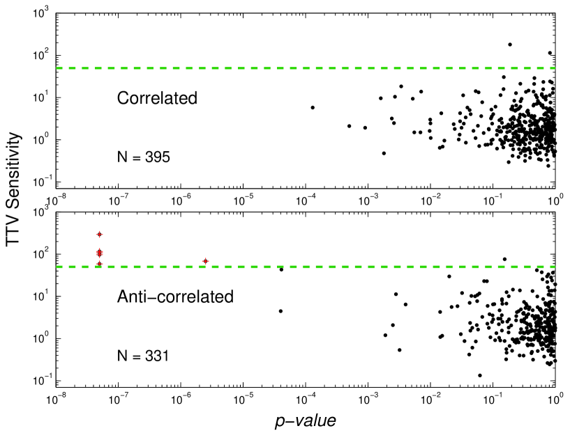
In order to single out the systems with significant correlation detection we picked out the KOIs that have a p-value lower than 10^-5. We found six such KOIs with negative $\mathcal{GS}$, suggesting a prograde configuration, while not a single system with positive $\mathcal{GS}$. In fact, we did not find any system with a positive $\mathcal{GS}$ and a p-value below 10^-4. These six KOIs with significant correlation are marked in the figure by red crosses, and are discussed in detail in Section 4.

One would expect to find systems showing a strong correlation (or anti-correlation) due to spot-crossings in the upper left corner, with high sensitivity and low p-value. Indeed, we find the six KOIs with significant correlation in that corner in the lower panel, while the same corner in the upper panel is empty. For five out of these systems all our $10^{7}$ random permutations gave a $\mathcal{GS}/\sigma_{\mathcal{GS}}$ smaller (in absolute value) than that of the real data, so somewhat arbitrarily we assigned them a p-value of 5$\cdot$10^-8 in Figure 1. We also find three other KOIs with high sensitivity (above the dashed line in both panels of Figure 1) but with no significant detection. The nine systems and their parameters are listed in Table 3. This includes the stellar effective temperature $T_{\rm eff}$, taken from the NASA Exoplanet Archive on December 1st, 2014, and the impact parameter $b$ of the planetary orbit, derived here as described in Section 3.

Table 3: Statistical parameters of the KOIs with high TTV sensitivity

KOI	Period	Depth	Period	Amp.	$\mathcal{GS}$	$\sigma_{\mathcal{GS}}$	p-($\mathcal{GS}/\sigma_{\mathcal{GS}}$)	Expected	$\sigma_{TTV}$	N	$\mathcal{S}$	$T_{\rm eff}$	$b$
	Orb.		Rot.		Rot.			TTV
	[d]	[ppm]	[d]	[ppm]	[min d]	[min d]	[log]	[min]	[min]			[K]
$3.01$	$4.89$	$4361$	$29.47$	$5875$	$26$	$19$	$-0.7$	$2.97$	$0.24$	$214$	$178.8$	$4777$	$0.28$
$63.01$	$9.43$	$4037$	$5.41$	$8910$	$2$	$10$	$-0.1$	$4.27$	$0.44$	$139$	$114.9$	$5650$	$0.73$
$203.01$	$1.49$	$21575$	$12.16$	$12865$	$-33$	$3$	$<-7$	$3.20$	$0.29$	$710$	$292.1$	$5624$	$0.24$
$217.01$	$3.91$	$22620$	$19.77$	$4970$	$-140$	$20$	$<-7$	$1.46$	$0.45$	$331$	$58.4$	$5543$	$0.26$
$254.01$	$2.46$	$40367$	$15.81$	$10930$	$-9$	$6$	$-0.8$	$1.57$	$0.48$	$540$	$75.4$	$3820$	$0.57$
$883.01$	$2.69$	$39186$	$9.02$	$11340$	$-38$	$4$	$<-7$	$1.94$	$0.40$	$495$	$107.1$	$4809$	$0.51$
$895.01$	$4.41$	$13822$	$5.07$	$10575$	$-39$	$5$	$<-7$	$5.33$	$0.95$	$302$	$97.0$	$5600$	$0.37$
$1074.01$	$3.77$	$14018$	$4.04$	$8360$	$-32$	$6$	$-5.6$	$4.12$	$1.04$	$296$	$67.9$	$6302$	$0.36$
$1546.01$	$0.92$	$15752$	$0.91$	$7600$	$-27$	$1$	$<-7$	$1.90$	$0.62$	$1430$	$115.6$	$5713$	$0.67$

3 The impact parameter and its impact on the correlation

As discussed and demonstrated in the simulations of Paper I, the TTV local-slope correlation can be detected only if the spot crossing events occur in varying locations on the stellar disc. This can happen only if the chords of the planet and the spot lie across the stellar disc side by side. If the latitude of the spot, $\theta$, is such that $\cos\theta$ is substantially different from the impact parameter of the transiting planet, or if the stellar obliquity is substantially different from zero (or from 180^∘), there cannot be any observed correlation. It is therefore of interest to examine the impact parameters of the systems with high sensitivity and see if the information about the planet motion over the stellar disc can tell us something about the location of the stellar spots. This discussion does not include KOI-1546, which was recently identified to be an eclipsing stellar binary.

We decided not to use the NASA Exoplanet Archive catalog values for the impact parameters of the KOIs, as they are based on long cadence data only, whereas short cadence data are available for all our high sensitivity systems. Furthermore, the KOI sample on the NASA Exoplanet Archive displays an impact parameter distribution with a strong increase towards $b=0$ (at the time of writing), instead of the expected uniform distribution. We do not know the cause for this artifact, but it suggests the use of those values may be unreliable for our tests.

Therefore, we derived the impact parameters ourselves for the eight systems, using the short cadence simple-aperture photometry data. The first step was detrending the transit light curve by finding the continuum around each transit, ignoring the photometry of the transit itself, up to 0.6 transit durations around the expected transit center. We then fitted a more extended region, of up to four durations around the expected transit center, and fitted six different polynomials of degrees one to six. An $\mathcal{F}$-test was performed between all of the different pairs of polynomial fits. The best fit was chosen as the one with the highest degree, for which the $p$-value of all the $\mathcal{F}$-tests with polynomial fits of lower degrees was lower than $10^{-3}$. The last stage of the detrending process was to add back the transit points and divide the flux at that region by the chosen polynomial fit.

To obtain a model for the transit we folded the light curves of the different transits together using the best-fitting period and phase. We then modeled the transit using the occultnl model (Mandel & Agol, 2002), where the position of the planet was chosen with a rectilinear model of normalized impact parameter $b$, transit duration $T_{\rm dur}$ from mid-ingress to mid-egress, a linear limb darkening law with parameter $c_{2}$ (and other $c_{i}$ of Mandel & Agol (2002) fixed to zero), and planet-to-star radius ratio $R_{p}/R_{\star}$. The model assumed no third light for the eight systems, consistent with the small contamination ($\lesssim 10\%$) reported at the MAST.

The fit was performed via the non-linear fitter IDL/mpfit (Markwardt, 2009). The scatter of out-of-transit points, $\sigma$, was used to determine the uncertainty of the individual measurements, instead of relying on the reported photometric errors. Ten iterations of the fitter were run, followed by rejection of points lying more than $10\sigma$ away from the model; this procedure was repeated; and a final ten iterations of the fitter resulted in the impact parameters reported in Table 3 and plotted in Figure 2. The reduced $\chi^{2}$ varied from $0.99$ to $1.78$ with a mean of $1.23$—these moderately exceed what white noise would have given, and they may be due to the scatter induced by the star spot crossing events.

Figure 2: Sensitivity to the correlation of TTV induced by spot-crossing with the brightness slope, $\mathcal{S}$, vs. the derived impact parameter of their transiting planet. Impact parameter was derived from the short cadence data, using the Mandel & Agol (2002) model. For some systems the error bar of the impact parameter is smaller than the marker size. The red points are the KOIs with detected correlation, with p-value lower than 10^-5, and the blue points are the systems with no significant detection of a correlation.

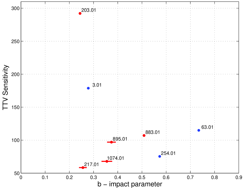
Figure 2 shows that the impact parameters of the five systems displaying TTV correlated with the local slope are in the range of $0.2\lesssim b\lesssim 0.5$. Interestingly, the Sun’s spots reach up to about $30^{\circ}$ in latitude, and their size grows smaller as they descend in latitude until reaching the equator when the Sun’s activity cycle is at minimum (e.g., Wilson et al., 1996; Li et al., 2000). Therefore, to an observer viewing the Sun from the equator plane, transiting planets would cross sunspots only if they have $b\leq 0.5$, and would be difficult to detect at $b\approx 0$, just as we see in these systems.

The only system with high sensitivity and $b\leq 0.5$ that does not show detected correlation is KOI-3.01 (= Kepler-3b = HAT-P-11b; Bakos et al. 2010; Winn et al. 2010b; Hirano et al. 2011; Sanchis-Ojeda & Winn 2011; see also Béky et al. 2014). This may be accounted for by the large stellar obliquity of KOI-3.01, as explained in more details in Section 5. A similar scenario might account for the lack of a correlation for KOI-63.01 (= Kepler-63b; Sanchis-Ojeda et al. 2013). For KOI-254.01 (= Kepler-45b; Johnson et al. 2012) there is no evidence for correlation and therefore for spot crossings, which might be explained by the relatively large impact parameter, beyond 0.5, that causes the planet to move across the stellar disk at higher latitudes than the spots. These three systems (KOI-3.01, KOI-63.01, and KOI-254.01) are reviewed in more details in Section 5.

Taken together, although extremely small, our sample suggests that the stars considered here have spots within $\approx 30^{\circ}$ of their equator but not exactly along the equator, in analogy to sunspots. However, this does not exclude the existence of high latitude star spots (e.g., Li et al., 2000) since our method is less sensitive to such systems. This is so because as the spot moves to higher latitude both the stellar photometric modulation amplitude and transit timing precision decrease.

In the next two sections we present the detailed analysis of the KOIs with high sensitivity. Section 4 discusses the systems with significant correlation, and Section 5 discusses the systems with non-significant correlation.

4 The six KOIs with significant correlation

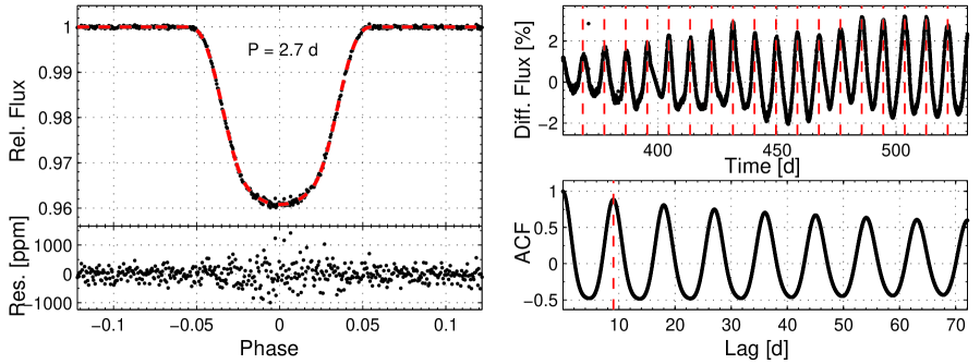
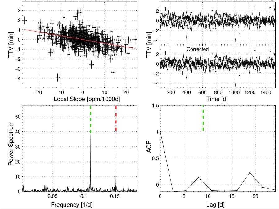
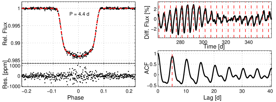
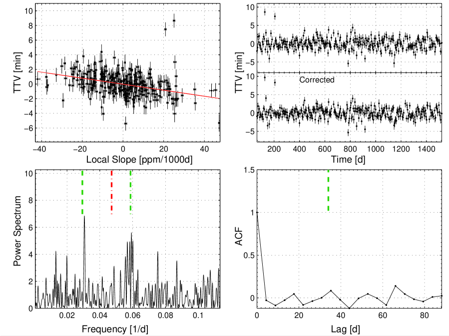
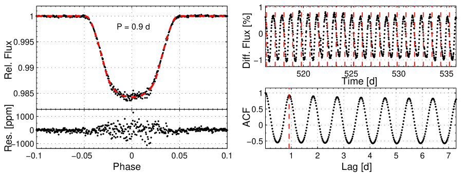
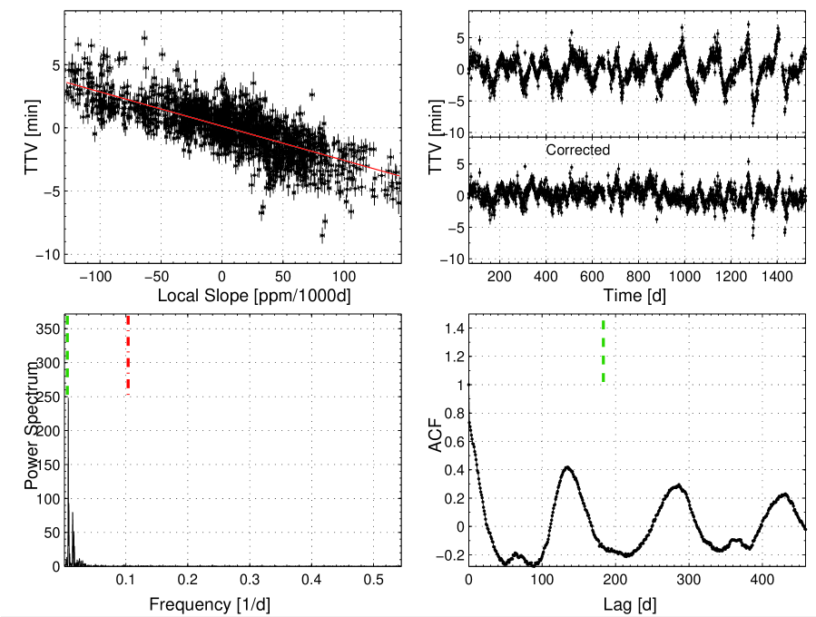
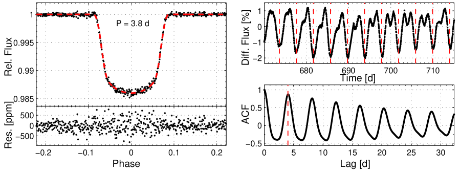
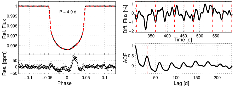
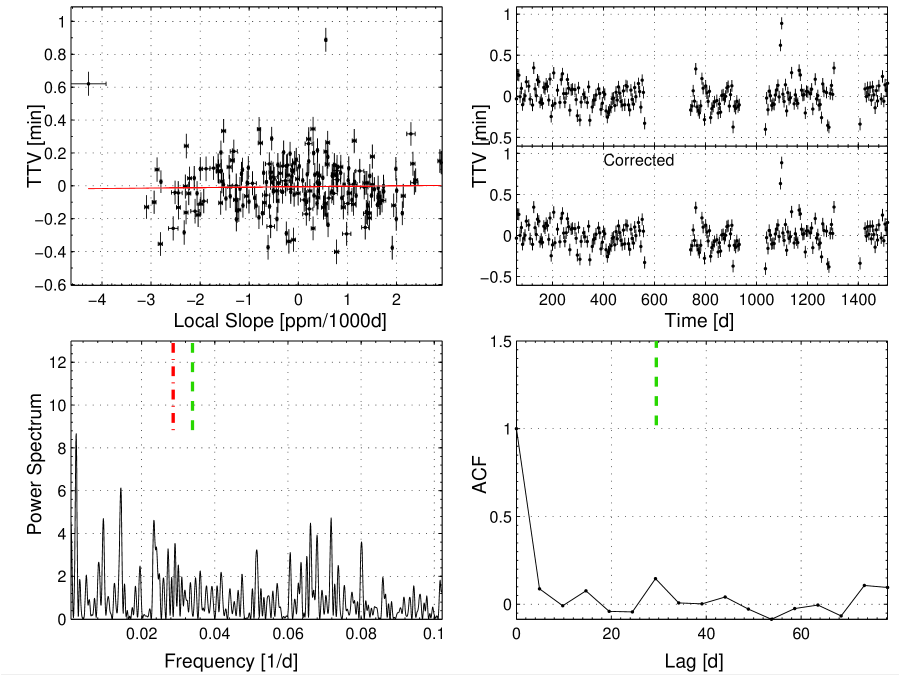
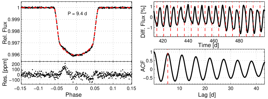
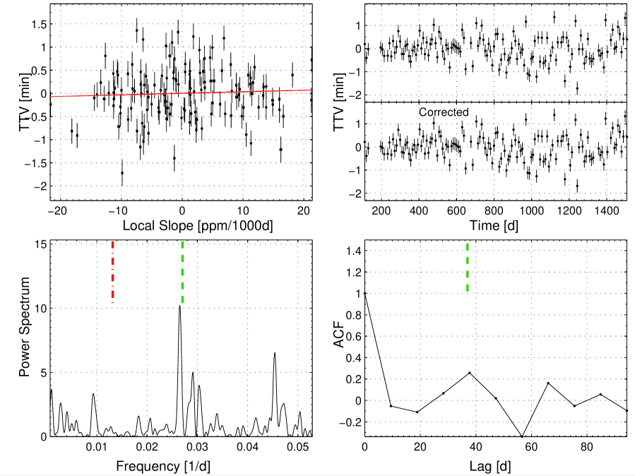
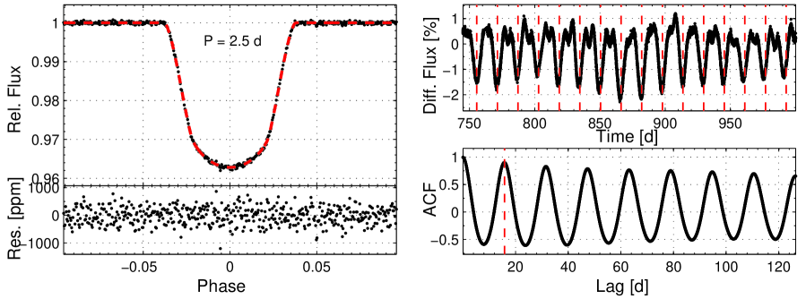
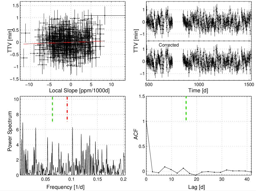
In this section we present the six systems that show a highly significant anticorrelation between their TTV and the corresponding local slope, with $\mathcal{GS}/\sigma_{\mathcal{GS}}$ p-value lower than 10^-5. Their analysis, based on the long cadence, are presented in Figures 3–14. Figures 3, 5, 7, 9, 11 and 13 show the light curve analysis, and Figures 4, 6, 8, 10, 12 and 14 show the TTV analysis.

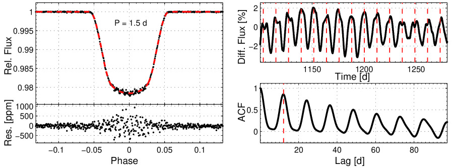
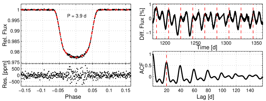
In Figures 3, 5, 7, 9, 11 and 13, the left panel presents the phase folded light curve around the transit, overplotted by the fitted model (red dashed line), with the residuals at the bottom. In all six systems, the larger scatter in the residuals during transit compared to out of transit is probably due to spot-crossing events.

The top right panel presents a segment of the light curve as a function of time, where the photometric modulation due to stellar rotation and activity is clearly noticeable. We can see that the modulation is not strictly periodic, as the spots evolve in size and location. The spacing between the vertical red dashed lines is the rotation period identified by McQuillan, Mazeh & Aigrain (2013, 2014). They used the Auto-Correlation Function (ACF), presented in the bottom right panel, where the red dashed line marks the rotation period, which, as expected, coincides with the shortest time lag ACF peak.

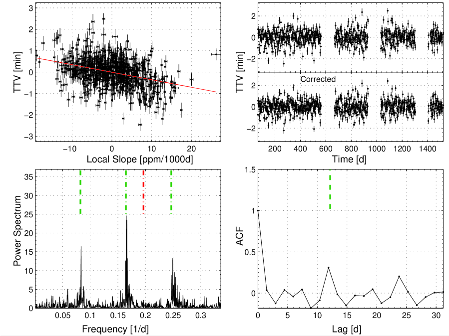
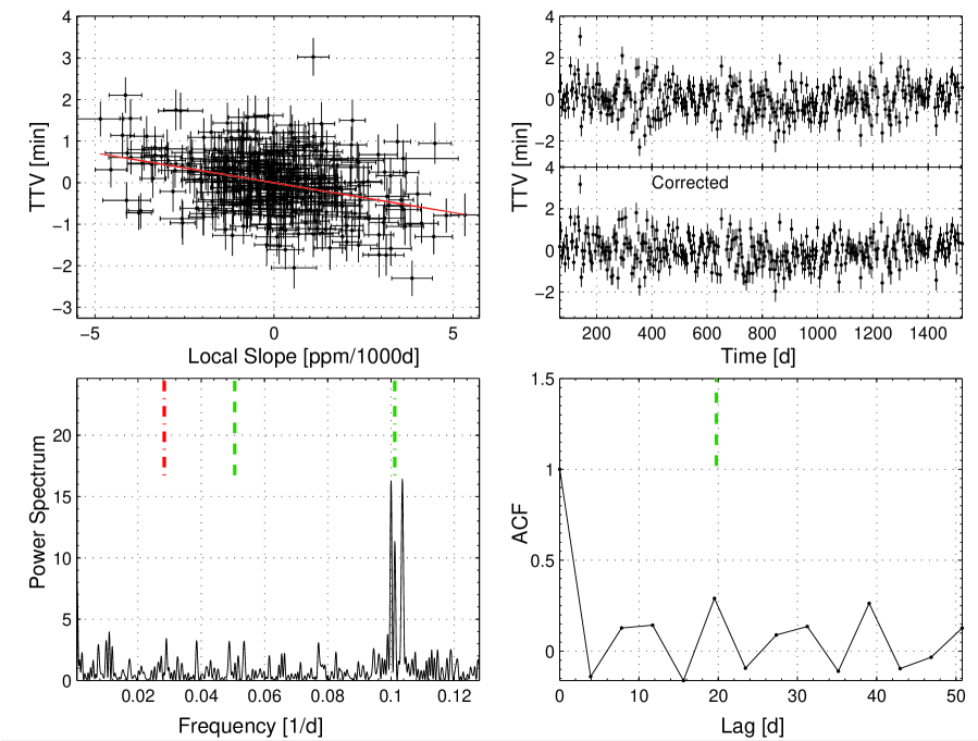
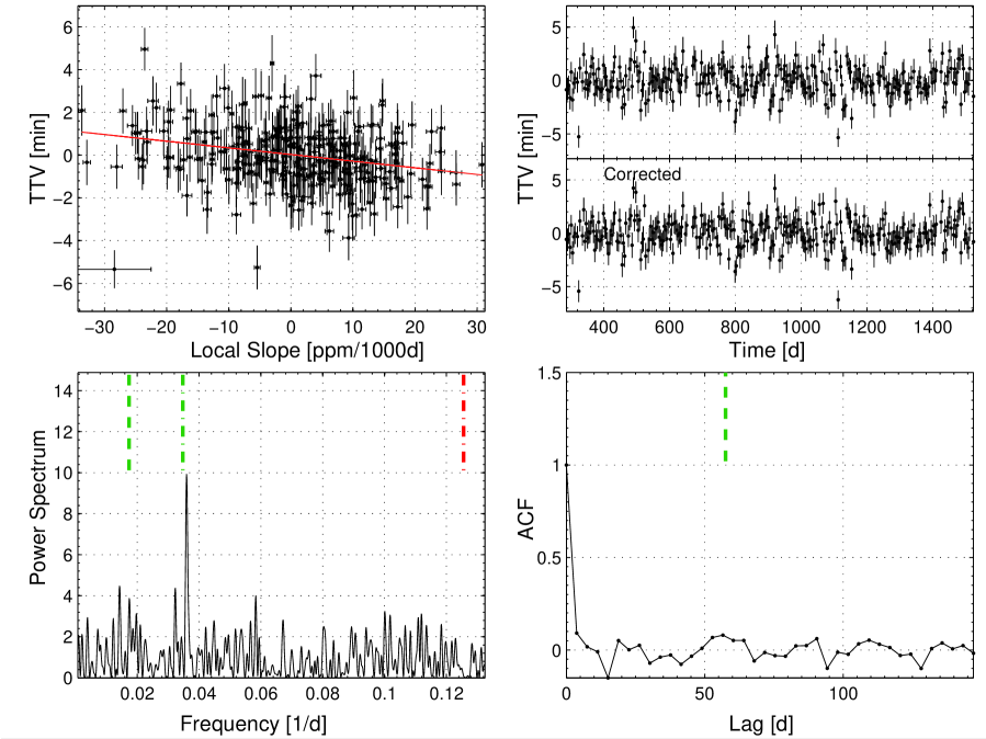
In Figures 4, 6, 8, 10, 12 and 14, the top left panel shows the TTV vs. the local photometric slope with the linear fit overplotted as a solid red line. The clear anti-correlation between the TTV and the local slope indicates prograde motion. The top right panel shows the measured TTV as a function of time (top) and the corrected TTV (bottom) after subtracting the linear fit of the TTV vs. local slope. The corrected TTV does not show much difference relative to the measured TTV (except maybe in KOI-1546.01).

The bottom left panel shows the TTV frequency power spectrum, with a green dashed line marking the stellar rotation frequency. When relevant, another green dotted-dashed line or two mark the harmonics of this frequency. The red dotted-dashed line marks the sampling stroboscopic frequency—the TTV signal induced by the sampling of the Kepler long cadence data (Szabó et al., 2013; Mazeh et al., 2013). The power spectrum is plotted up to the Nyquist frequency, which in this case is half the orbital frequency, at which the TTV signal is sampled. The bottom right panel shows the TTV ACF with the stellar rotation period marked by a green dashed line.

In two cases, KOI-203 and KOI-883, we see a clear TTV periodicity with the rotational period. This is another indication that the TTV signal is related to the stellar rotation. In the case of KOI-217.01 and KOI-1074 (Figures 6 and 14) the strongest power spectrum (PS) peak is at twice the stellar rotation frequency. This is consistent with a scenario in which the star has two significant spots (or groups of spots), each at opposite hemispheres, as can be seen also in the stellar light curves (Figures 5 and 13 top right panel).

Note that for KOI-895, KOI-1074, and KOI-1546.01, the rotational frequency $f_{\rm rot}$ is larger than the Nyquist frequency of the sampling, which is half the orbital frequency, $f_{\rm Nyq}=0.5f_{\rm orb}$ (see the orbital and rotation periods listed in Table 3). Therefore the rotational frequency is aliased to a smaller frequency.

Out of the six KOIs, two are confirmed planet hosts. KOI-$203.01$ (Figure 3) was confirmed by Désert et al. (2011, Kepler-17b), who used Kepler short cadence data and found it to be prograde with a spin-orbit angle smaller than 15^∘, which agrees well with our findings. The second confirmed planet is KOI-217.01 (Howell et al., 2010, Kepler-71b).

5 KOIs with no significant correlation

In this section we present the three KOIs with high sensitivity but with no detected correlation between the TTV and the corresponding local-slope. All three, KOI-3.01 (= Kepler-3b = HAT-P-11b; Bakos et al. 2010), KOI-63.01 (= Kepler-63b; Sanchis-Ojeda et al. 2013), and KOI-254.01 (= Kepler-45b; Johnson et al. 2012) are confirmed planets. They are presented in Figures 15 through 20 in the same format as the KOIs showing significant correlation (see Section 4 and Figures 3 through 14). It can be visually seen that the TTV vs. local slope does not show a significant correlation for all three systems (see Figures 16, 18, and 20).

In order to allow a more careful examination of the light curves of these three systems, and specifically to try and understand why they do not show a significant correlation, we use here the Kepler short cadence data and the Mandel & Agol (2002) transit model for generating Figures 15 through 20.

For KOI-3.01 (= Kepler-3b = HAT-P-11b; see Figures 15 and 16) the residuals of the phase folded and binned light curve are not consistent with white noise but instead show clear systematic features (Figure 15 left panel). This is in contrast to the other systems (see Figures 3, 5, 7, 9, 11, and 13) where the residuals of the in-transit light curve show an increased noise level but no systematic features. This distribution of the residuals suggests that the same features occur in many transit events at the same phases, so they do not average out in the folded light curve. Assuming these residuals are caused by spot-crossing events, this might suggest that the spot crossings occur primarily at specific phases during the transit.

Fortunately, the Kepler light curve of KOI-3.01 was carefully studied by several authors (Sanchis-Ojeda & Winn, 2011; Deming et al., 2011; Béky et al., 2014), in addition to observations of the RM effect (Winn et al., 2010b; Hirano et al., 2011). These studies found that the system has a sky-projected spin-orbit angle close to 90^∘, and that the host star has two active latitudes. Hence, spot-crossing events occur when the planet moves across the active stellar latitudes, explaining why they are seen only at specific phases during the transit. Since those phases sample only part of the transit and not the entire transit it reduces the TTV range induced by the spot-crossing events. This is also consistent with a weak TTV periodicity identified at the rotation period (see Figure 16), where no significant peak is seen at the rotation frequency (bottom left panel) and only a small peak, close to the noise level at the ACF (bottom right panel). Moreover, in this configuration, when a spot is crossed by the planet the star is at a similar phase in its rotation, resulting in a small range of local slopes. The combined result is that although this system posses the sensitivity for TTV–local-slope correlation, its characteristics suppress that correlation.

KOI-63.01 (= Kepler-63b; see Figures 17 and 18) also shows systematic features in the phase folded light curve residuals (Figure 17 left panel). Sanchis-Ojeda et al. (2013) have already studied the Kepler-63b Kepler light curve and observed the RM effect. They determined the system has a sky-projected spin-orbit misalignment of -110${}^{+22}_{-14}$ deg and a stellar spin axis inclination angle of 138$\pm$7 deg. Therefore, in this configuration the spot-crossing events are confined to the same parts of the transit. This explains the features in the phased light curve residuals and the non-detection of a spots-induced TTV signal, where the latter leads to no TTV–local-slope correlation. Yet, the TTV period analysis (Figure 18) does show a significant TTV periodicity at the rotation frequency, which in this case is aliased to $f_{\rm rot,alias}=2f_{\rm orb}-f_{\rm rot}$, as $3f_{\rm Nyq}<f_{\rm rot}<4f_{\rm Nyq}$. This could be explained by assuming there are one or two spot latitudes and therefore one or two transit phases that allow spot crossing, not enough to produce a detectable correlation, but enough to induce a TTV modulation with the rotation period.

For KOI-254.01 (= Kepler-45b, Johnson et al. 2012; see Figures 19 and 20), the spin-orbit angle is currently not known. We hypothesize that the planet does not cross spots during the transit and that the system is spin-orbit aligned, similar to, e.g., Kepler-77 (Gandolfi et al., 2013). This is consistent with the noise level of the in-transit light curve being similar to the noise level of the out-of-transit phases, which is different from the six systems with significant correlation that show an increased in-transit residuals noise level (see Section 4 and Figures 3, 5, 7, 9, 11, and 13). For this system we have determined here a transit impact parameter of 0.5732 $\pm$ 0.0027, consistent with Johnson et al. 2012 value of 0.6 $\pm$ 0.2, who used less Kepler data than used here. This impact parameter is larger than the ones of the systems with significant correlation (see Figure 2), suggesting that KOI-254.01 impact parameter is larger than the impact parameter corresponding to the typical active stellar latitudes. For this object the TTV period analysis (Figure 20) does not show a periodicity at the rotation period, as expected.

Another possible scenario that can weaken the correlation between the TTV and the local slope and was not mentioned above is a dynamical TTV signal, following the gravitational interaction with another body in the systems (e.g., Fabrycky et al., 2012; Ford et al., 2012; Steffen et al., 2012). However, there is no evidence for such a signal in any of the three systems discussed above.

To summarize this section, for all three systems we are able to provide plausible scenarios that explain why despite having the sensitivity to a TTV signal induced by spot-crossing events, these systems do not show a detected correlation.

6 Discussion

We presented here the application of a simple method to distinguish between prograde and retrograde transiting star-planet systems, where the brightness of the host star is modulated by stellar spots, and the transits include spot-crossing events. The method is based on the assumption that even when spot-crossing events are not resolved, they induce a shift in the derived mid-transit timing, when fitting a model that ignores the spot-crossings. We have applied our method to a sample of 2,600 KOIs whose transit timings were measured by Holczer et al. (2015, in preparation) using the long cadence data, and are publicly available (ftp://wise-ftp.tau.ac.il/pub/tauttv/TTV/ver$\_$112). We have concentrated on 862 systems with published stellar rotation periods (McQuillan, Mazeh & Aigrain, 2013, 2014), out of which only 726 had at least 20 measurements of the TTV and local slope.

Using the formalism of Paper I, we identified nine systems, listed in Table 3, with high enough stellar modulations and large enough planets to allow the detection of the TTV local-slope correlation. The nine systems have relatively large photometric modulation amplitudes due to rotation ($\gtrsim 5000$ ppm), all of them well above the median of the whole analyzed sample ($\sim$3000 ppm). The precision of the transit timing for these nine systems is high, with a median of 0.45 min, while the sample median is $\sim$13 min. This indicates that our method requires objects showing relatively strong rotation modulation and high SNR transits, the latter leading to highly precise mid-transit timings. The nine systems we have identified have orbital periods in the range of 0.9–9.4 d and transit depth of 0.4–4.0%, consistent with the typical parameters range of hot Jupiters. The small size of the sample is not surprising, given the fact that we are looking for a minor effect that is hiding in the noise in most cases. One of the nine cases is KOI-1546, which recently has been found to be a stellar binary, so we are left with eight bona fide planet-candidate systems (five of which already confirmed as planets).

It turned out that out of these eight systems five show a clear negative correlation, indicating prograde motion, and none a positive correlation, which could have indicated a retrograde motion. This is consistent with the finding of the seminal work of Winn et al. (2010a), who showed that most cool planet-host stars have close to zero obliquity, as four out of our five systems have lower surface temperature. However, this could also result from an intrinsic bias in our approach, since it requires active host stars, which are typically convective and hence relatively cold.

As shown in Figure 2, the five systems with detected correlation (not including KOI-1546, which is a binary) all have an impact parameter in the range of $0.2\lesssim b\lesssim 0.5$. Assuming those systems have their spots moving on similar latitudes as the planetary chord as seen from Earth, this result shows a similarity to the Sun, where the spots reach up to about $30^{\circ}$ latitude and decrease in the size as they move closer to the Sun’s equator.

To summarize, we have found evidence for prograde motion of transiting planets but no retrograde motion. Furthermore, we found some hints that stellar spots might preferentially be at low, Sun-like, latitudes on the stellar disc ($<30^{\circ}$) but not exactly along the stellar equator, although our search suffers from an observational bias against detection of high latitude spots, and the detected sample is extremely small. The original goal of this project was to learn about the planetary motion, but we were surprised to find a possible hint about a feature of spot motion. In principle this is possible, as the planet with its small radius is sampling the stellar surface with high resolution that is not available in present-day observational techniques. The high precision, evenly spaced, long-span light curves of Kepler make this possible.

The approach described here is not limited to Kepler star-planet systems and can, in principle, be applied to Kepler stellar binary systems (Prša et al., 2011; Slawson et al., 2011), an analysis that we are preparing in a forthcoming paper. In fact, a negative correlation between TTV and local slope was identified already for the eclipsing stellar binary system within the circumbinary planetary system Kepler-47 (Orosz et al., 2012), where a more detailed analysis of the spot-crossing events indicates a prograde motion (Orosz et al., 2012).

In the future the method used here can be applied to a large sample of systems monitored by current and future space-based surveys delivering high-quality photometry, including K2 (Howell et al., 2014), TESS (Ricker et al., 2014), and PLATO (Rauer et al., 2014). A larger sample can reveal the typical characteristics of prograde and retrograde systems, which in turn will allow constraining formation and orbital evolution processes. In addition, a larger sample of systems where spot-crossing events are identified will also better constrain spots’ behavior.

Figure 3: KOI-203.01 (= Kepler-17b): Transit light curve and stellar modulation and its autocorrelation. Left: Model fit to the detrended phase folded transit light curve (top) and its residuals (bottom, in ppm). The fitted model is overplotted in a red dashed line. Upper right: A segment of the light curve. The spacing between the vertical red dashed lines equals the host star’s rotation period. One can follow the stellar rotation modulation with the detected period. The modulation changes its shape and amplitude, but retains its period. Bottom right: The Auto-Correlation Function (ACF), with a vertical red dashed line where the rotation period is found. One can clearly see the ACF peaks at lags equal to integer multiples of the rotation period.

Figure 4: Analysis of the TTV of KOI-203.01 (= Kepler-17b). Upper left: The TTV, in minutes, as a function of the corresponding local slope, in ppm per thousand days. The overplotted solid line (red) is a linear fit whose slope is defined as the global slope. Upper right: The derived TTVs as function of time. The upper panel shows the derived TTV, while the lower panel displays the corrected one, after subtracting the linear fit plotted in upper left panel. Bottom left: The TTV power spectrum. One can clearly see strong peaks corresponding to the stellar rotation period, marked by a green dashed line, and its first two harmonics, marked by green dotted-dashed lines. The red dotted-dashed line marks the sampling stroboscopic frequency which is the TTV signal induced by the sampling of the Kepler long cadence data (Szabó et al., 2013; Mazeh et al., 2013). The power spectrum is plotted up to the Nyquist frequency which in this case is half the orbital frequency. Bottom right: The ACF of the derived TTV. The green dashed line presents the lag corresponding to the stellar rotation. One can notice a small peak at this lag and another one at a lag twice the rotation period.

Figure 5: KOI-217.01 (= Kepler-71b) transit light curve and stellar modulation and its autocorrelation. See Figure 3 for details.

Figure 6: Analysis of the TTV of KOI-217.01 (= Kepler-71b). See Figure 4 for details. The green dashed line in the bottom left panel mark the stellar rotation frequency, and its first harmonic is marked by a green dotted-dashed line.

Figure 7: KOI-883.01 transit light curve and stellar modulation and its autocorrelation. See Figure 3 for details.

Figure 8: Analysis of the TTV of KOI-883.01. See Figure 4 for details. The green dashed line in the bottom left panel marks the stellar rotation frequency.

Figure 9: KOI-895.01 transit light curve and stellar modulation and its autocorrelation. See Figure 3 for details.

Figure 10: Analysis of the TTV of KOI-895.01. See Figure 4 for details. The green dashed line in the bottom left panel mark the stellar rotation frequency, and its first harmonic is marked by a green dotted-dashed line.

Figure 11: KOI-1546.01 transit light curve and stellar modulation and its autocorrelation. See Figure 3 for details.

Figure 12: Analysis of the TTV of KOI-1546.01. See Figure 4 for details. The green dashed line in the bottom left panel marks the stellar rotation frequency.

Figure 13: KOI-1074.01 transit light curve and stellar modulation and its autocorrelation. See Figure 3 for details.

Figure 14: Analysis of the TTV of KOI-1074.01. See Figure 4 for details. The green dashed line in the bottom left panel mark the stellar rotation frequency, and its first harmonic is marked by a green dotted-dashed line.

Figure 15: KOI-3.01 transit light curve and stellar modulation and its autocorrelation. See Figure 3 for details.

Figure 16: Analysis of the TTV of KOI-3.01. See Figure 4 for details. The green dashed line in the bottom left panel mark the stellar rotation frequency.

Figure 17: KOI-63.01 transit light curve and stellar modulation and its autocorrelation. See Figure 3 for details.

Figure 18: Analysis of the TTV of KOI-63.01. See Figure 4 for details. The green dashed line in the bottom left panel mark the stellar rotation frequency.

Figure 19: KOI-254.01 transit light curve and stellar modulation and its autocorrelation. See Figure 3 for details.

Figure 20: Analysis of the TTV of KOI-254.01. See Figure 4 for details. The green dashed line in the bottom left panel mark the stellar rotation frequency.

References

- Albrecht et al. (2012) Albrecht, S., Winn, J. N., Johnson, J. A., et al. 2012, ApJ, 757, 18
- Albrecht et al. (2013) Albrecht, S., Winn, J. N., Marcy, G. W., et al. 2013, ApJ, 771, 11
- Bakos et al. (2010) Bakos, G. Á., Torres, G., Pál, A., et al. 2010, ApJ, 710, 1724
- Barnes (2009) Barnes, J. W. 2009, ApJ, 705, 683
- Barnes et al. (2011) Barnes, J. W., Linscott, E., & Shporer, A. 2011, ApJS, 197, 10
- Batygin (2012) Batygin, K. 2012, Nature, 491, 418
- Béky et al. (2014) Béky, B., Holman, M. J., Kipping, D. M., & Noyes, R. W. 2014, ApJ, 788, 1
- Chaplin et al. (2013) Chaplin, W. J., Sanchis-Ojeda, R., Campante, T. L., et al. 2013, ApJ, 766, 101
- Cresswell et al. (2007) Cresswell, P., Dirksen, G., Kley, W., & Nelson, R. P. 2007, A&A, 473, 329
- Dawson (2014) Dawson, R. I. 2014, ApJ, 790, LL31
- Deming et al. (2011) Deming, D., Sada, P. V., Jackson, B., et al. 2011, ApJ, 740, 33
- Désert et al. (2011) Désert, J.-M., Charbonneau, D., Demory, B.-O., et al. 2011, ApJS, 197, 14
- Van Eylen et al. (2014) Van Eylen, V., Lund, M. N., Silva Aguirre, V., et al. 2014, ApJ, 782, 14
- Fabrycky & Tremaine (2007) Fabrycky, D., & Tremaine, S. 2007, ApJ, 669, 1298
- Fabrycky & Winn (2009) Fabrycky, D. C., & Winn, J. N. 2009, ApJ, 696, 1230
- Fabrycky et al. (2012) Fabrycky, D. C., Ford, E. B., Steffen, J. H., et al. 2012, ApJ, 750, 114
- Ford et al. (2012) Ford, E. B., Fabrycky, D. C., Steffen, J. H., et al. 2012, ApJ, 750, 113
- Gandolfi et al. (2013) Gandolfi, D., Parviainen, H., Fridlund, M., et al. 2013, A&A, 557, A74
- Gaudi & Winn (2007) Gaudi, B. S., & Winn, J. N. 2007, ApJ, 655, 550
- Gizon & Solanki (2003) Gizon, L., & Solanki, S. K. 2003, ApJ, 589, 1009
- Groot (2012) Groot, P. J. 2012, ApJ, 745, 55
- Hébrard et al. (2011) Hébrard, G., Ehrenreich, D., Bouchy, F., et al. 2011, A&A, 527, L11
- Hirano et al. (2011) Hirano, T., Narita, N., Shporer, A., et al. 2011, PASJ, 63, 531
- Hirano et al. (2012) Hirano, T., Sanchis-Ojeda, R., Takeda, Y., et al. 2012, ApJ, 756, 66
- Hirano et al. (2014) Hirano, T., Sanchis-Ojeda, R., Takeda, Y., et al. 2014, ApJ, 783, 9
- Holczer et al. (2015, in preparation) Holczer, T., et al., 2015, in preparation
- Howell et al. (2010) Howell, S. B., Rowe, J. F., Sherry, W., et al. 2010, ApJ, 725, 1633
- Howell et al. (2014) Howell, S. B., Sobeck, C., Haas, M., et al. 2014, PASP, 126, 398
- Johnson et al. (2012) Johnson, J. A., Gazak, J. Z., Apps, K., et al. 2012, AJ, 143, 111
- Li et al. (2000) Li, K., Gu, X., Xiang, F., Liu, X., & Chen, X. 2000, MNRAS, 317, 897
- Lund et al. (2014) Lund, M. N., Lundkvist, M., Silva Aguirre, V., et al. 2014, A&A, 570, A54
- Mandel & Agol (2002) Mandel, K., & Agol, E. 2002, ApJ, 580, L171
- Markwardt (2009) Markwardt, C. B. 2009, Astronomical Data Analysis Software and Systems XVIII, 411, 251
- Mazeh et al. (2013) Mazeh, T., Nachmani, G., Holczer, T., et al. 2013, ApJS, 208, 16
- Mazeh et al. (2015a) Mazeh, T., Holczer, T., & Shporer, A. 2015a, ApJ, 800, 142 (Paper I)
- Mazeh et al. (2015b) Mazeh, T., Perets, H. B., McQuillan, A., & Goldstein, E. S. 2015b, ApJ, 801, 3
- McQuillan, Mazeh & Aigrain (2013) McQuillan, A., Mazeh, T., & Aigrain, S. 2013, ApJ, 775, L11
- McQuillan, Mazeh & Aigrain (2014) McQuillan, A., Mazeh, T., & Aigrain, S. 2014, ApJS, 211, 24
- Morton & Winn (2014) Morton, T. D., & Winn, J. N. 2014, ApJ, 796, 47
- Nagasawa et al. (2008) Nagasawa, M., Ida, S., & Bessho, T. 2008, ApJ, 678, 498
- Naoz et al. (2011) Naoz, S., Farr, W. M., Lithwick, Y., Rasio, F. A., & Teyssandier, J. 2011, Nature, 473, 187
- Nutzman et al. (2011) Nutzman, P. A., Fabrycky, D. C., & Fortney, J. J. 2011, ApJ, 740, L10
- Orosz et al. (2012) Orosz, J. A., Welsh, W. F., Carter, J. A., et al. 2012, Science, 337, 1511
- Oshagh et al. (2013) Oshagh, M., Santos, N. C., Boisse, I., et al. 2013, A&A, 556, A19
- Prša et al. (2011) Prša, A., et al. 2011, AJ, 141, 83
- Rauer et al. (2014) Rauer, H., Catala, C., Aerts, C., et al. 2014, Experimental Astronomy, 38, 249
- Ricker et al. (2014) Ricker, G. R., Winn, J. N., Vanderspek, R., et al. 2014, Proc. SPIE, 9143, 914320
- Sanchis-Ojeda et al. (2011) Sanchis-Ojeda, R., Winn, J. N., Holman, M. J., et al. 2011, ApJ, 733, 127
- Sanchis-Ojeda & Winn (2011) Sanchis-Ojeda, R., & Winn, J. N. 2011, ApJ, 743, 61
- Sanchis-Ojeda et al. (2012) Sanchis-Ojeda, R., Fabrycky, D. C., Winn, J. N., et al. 2012, Nature, 487, 449
- Sanchis-Ojeda et al. (2013) Sanchis-Ojeda, R., Winn, J. N., Marcy, G. W., et al. 2013, ApJ, 775, 54
- Schlaufman (2010) Schlaufman, K. C. 2010, ApJ, 719, 602
- Shporer et al. (2012) Shporer, A., Brown, T., Mazeh, T., & Zucker, S. 2012, New A, 17, 309
- Slawson et al. (2011) Slawson, R. W., Prša, A., Welsh, W. F., et al. 2011, AJ, 142, 160
- Steffen et al. (2012) Steffen, J. H., Fabrycky, D. C., Ford, E. B., et al. 2012, MNRAS, 421, 2342
- Szabo et al. (2011) Szabo, G. M., et al. 2011, ApJ, 736, 4
- Szabó et al. (2013) Szabó, R., Szabó, G. M., Dálya, G., et al. 2013, A&A, 553, A17
- Triaud et al. (2010) Triaud, A. H. M. J., Collier Cameron, A., Queloz, D., et al. 2010, A&A, 524, A25
- Wilson et al. (1996) Wilson, R. M., Hathaway, D. H., & Reichmann, E. J. 1996, J. Geophys. Res., 101, 19967
- Winn et al. (2010a) Winn, J. N., Fabrycky, D., Albrecht, S., & Johnson, J. A. 2010a, ApJ, 718, L145
- Winn et al. (2010b) Winn, J. N., Johnson, J. A., Howard, A. W., et al. 2010b, ApJ, 723, L223