Fast quantum non-demolition readout from longitudinal qubit-oscillator interaction

Abstract

We show how to realize high-fidelity quantum non-demolition qubit readout using longitudinal qubit-oscillator interaction. This is realized by modulating the longitudinal coupling at the cavity frequency. The qubit-oscillator interaction then acts as a qubit-state dependent drive on the cavity, a situation that is fundamentally different from the standard dispersive case. Single-mode squeezing can be exploited to exponentially increase the signal-to-noise ratio of this readout protocol. We present an implementation of this idea in circuit quantum electrodynamics and a possible multi-qubit architecture.

Introduction – Measurement in quantum information processors is generally realized by entangling a qubit to an ancillary system, with the states of the latter strongly depending on the qubit states. The ability to resolve these ancillary, or pointer, states can then result in a qubit measurement. This readout should be fast, quantum non-demolition (QND) and of high-fidelity. A common approach to realize this is the dispersive regime of cavity QED where the electric dipole moment of an atom strongly couples to the electric field of a high-Q cavity Haroche and Raimond (2006). In the dispersive regime where the qubit-cavity detuning $\Delta$ is large with respect to the coupling strength $g_{\mathrm{x}}$, the cavity frequency $\omega_{\mathrm{r}}$ is modified to take a qubit-state dependent value $\omega_{\mathrm{r}}\pm\chi$, with $\chi=g_{\mathrm{x}}^{2}/\Delta$ the dispersive qubit-cavity interaction. Starting in the vacuum state, a drive then displaces the cavity to qubit-state dependent coherent states $|\alpha_{0,1}\rangle$. Resolving these two pointer states by homodyne detection of the transmitted or reflected signal completes the qubit readout. Combined with recent advances in near quantum-limited amplification Castellanos-Beltran et al. (2008); Bergeal et al. (2010); Eichler and Wallraff (2014), this approach has led to high-fidelity readout with superconducting qubits Vijay et al. (2011, 2012); Hatridge et al. (2013); Jeffrey et al. (2014).

Figure 1: (a) Evolution in phase space of the cavity output field $\hat{a}_{\mathrm{out}}$ for longitudinal (full lines) and dispersive coupling (dashed lines, $\chi=\kappa/2$). Blue and red refer to qubit states. For the chosen parameters, the field starts at $(0,0)$ to reach $(0,\pm 1)$ in steady-state; the circles illustrate the position of the pointer states at characteristic times. Longitudinal coupling modulation and coherent drive are switched on as $(2/\pi)\arctan(10\kappa t)$. (b) Pointer state separation as a function of time. Vertical lines correspond to the circles of panel (a).

Despite these successes, current state-of-the-art dispersive readout suffers from several problems. First, readout must be made faster to meet the stringent requirements of fault-tolerant quantum computation Raussendorf and Harrington (2007). This is however challenging with the dispersive qubit-cavity interaction taking the form $H_{\mathrm{disp}}=\chi\hat{a}^{\dagger}\hat{a}\hat{\sigma}_{z}$. Indeed as illustrated by the dashed lines in Fig. 1(a) under this interaction a coherent drive at the input of the cavity first pushes the two pointer states in the same direction in phase space before pulling them apart. There is therefore little information about the qubit state at small measurement times. Second, $H_{\mathrm{disp}}$ derives in second-order perturbation theory from the electric-dipole interaction $g_{\mathrm{x}}(\hat{a}^{\dagger}+\hat{a})\hat{\sigma}_{x}$ Haroche and Raimond (2006). Since the latter does not commute with the measured qubit observable, $\hat{\sigma}_{z}$, dispersive readout is only QND in a perturbative sense. This non-QNDness manifests itself with Purcell decay $\gamma_{\kappa}=(g_{\mathrm{x}}/\Delta)^{2}\kappa$ Houck et al. (2008), where $\kappa$ is the cavity damping rate, and with the experimentally observed measurement-induced qubit transitions Boissonneault et al. (2009); Slichter et al. (2012). For this reason, the cavity damping rate cannot be made arbitrarily large and the measurement photon number $\bar{n}$ is typically kept well below the critical photon number $n_{\mathrm{crit}}=(\Delta/2g_{\mathrm{x}})^{2}$ Blais et al. (2004). Increasing $\kappa$ and $\bar{n}$ would otherwise lead to faster qubit measurement.

In this letter, we study an alternative approach that addresses both the slow measurement time and the non-QNDness. This proposal is based on a longitudinal qubit-cavity interaction of the form $g_{\mathrm{z}}(\hat{a}^{\dagger}+\hat{a})\hat{\sigma}_{z}$. As already noted in Refs. Kerman (2013); Billangeon et al. (2015), this coupling is purely QND and therefore avoids Purcell decay. Here, we show that under appropriate driving, longitudinal interaction leads to an optimal separation of the two pointer states in phase space, without the initial slow separation that is characteristic of the dispersive interaction. In contrast to the dispersive case Barzanjeh et al. (2014); Didier et al. (2015), we moreover find that the signal-to-noise ratio (SNR) of qubit readout can be exponentially improved by injecting a single-mode squeezed state in the cavity. As a possible realization of this idea, we discuss a circuit QED implementation based on a transmon qubit Koch et al. (2007) strongly coupled to the flux degree of freedom of an oscillator. The effect of imperfections and a possible multi-qubit architecture are also presented.

Longitudinal readout – Under longitudinal coupling, the qubit-cavity Hamiltonian reads ($\hbar=1$)

$$\hat{H}=\omega_{\mathrm{r}}\hat{a}^{\dagger}\hat{a}+\tfrac{1}{2}\omega_{\mathrm{a}}\hat{\sigma}_{z}+g_{\mathrm{z}}\hat{\sigma}_{z}(\hat{a}^{\dagger}+\hat{a}),$$ (1)

where $\omega_{\mathrm{r}}$ and $\omega_{\mathrm{a}}$ are respectively the cavity and qubit frequencies, while $g_{\mathrm{z}}$ is the longitudinal coupling strength. The realization of multi-qubit gates based on this interaction has already been discussed in the context of trapped ions Milburn et al. (2000); Sørensen and Mølmer (2000); Garcia-Ripoll et al. (2003); Leibfried et al. (2003) and superconducting qubits Blais et al. (2007); Kerman (2013); Billangeon et al. (2015). In particular, Ref. Kerman (2013) proposes to modulate the bias of a flux qubit to realize two-qubit gates. In the absence of external perturbations however, this interaction leads in steady-state to a qubit-state dependent displacement of the cavity field of amplitude $\pm g_{\mathrm{z}}/(\omega_{\mathrm{r}}+i\kappa/2)$. In other words, longitudinal interaction is of no consequences for the typical case where $\omega_{\mathrm{r}}\gg g_{\mathrm{z}},\kappa$.

Here we propose to render this interaction resonant for readout by modulating the coupling at the resonator frequency: $g_{\mathrm{z}}(t)=\bar{g}_{\mathrm{z}}+\tilde{g}_{\mathrm{z}}\cos(\omega_{\mathrm{r}}t)$. In the interaction picture and neglecting fast-oscillating terms we obtain

$$\tilde{H}=\tfrac{1}{2}\tilde{g}_{\mathrm{z}}\hat{\sigma}_{z}(\hat{a}^{\dagger}+\hat{a}).$$ (2)

This now leads to a large qubit-state dependent displacement $\pm\tilde{g}_{\mathrm{z}}/\kappa$. Even with a conservative modulation amplitude $\tilde{g}_{\mathrm{z}}\sim 10\kappa$, the steady-state displacement corresponds to 100 photons and the two qubit states are easily distinguishable by homodyne detection. We note that with this longitudinal coupling there is no concept of critical photon number and large intra-cavity photon population is therefore not expected to perturb the qubit.

Figure 2: (a) SNR in units of $\tilde{g}_{\mathrm{z}}/\kappa$ as a function of integration time $\tau$. Longitudinal coupling (green line) is compared to dispersive coupling (dashed black line, $\chi=\kappa/2$) for the same pointer state separation, $|\tilde{g}_{\mathrm{z}}|=|\epsilon|$. The dotted cyan line accounts for a residual dispersive coupling of $\chi=\kappa/5$. The full brown line shows the exponential improvement obtained for a single-mode squeezed input state with $e^{2r}=20\,\mathrm{dB}$. (b) Integration time $\tau$ required to achieve a fidelity $F=99.99\,\%$ versus longitudinal coupling. (c) Cavity damping rate to reach a fidelity of 99.99% in 50 ns versus intra-cavity photon number $\bar{n}=(g_{\mathrm{z}}/\kappa)^{2}=2(\epsilon/\kappa)^{2}$. Squeezing (full brown line) helps in further reducing the required photon number or cavity decay rate. The squeeze strength is optimized for each $\kappa$, with a maximum set to 20 dB reached close to $\kappa/2\pi=1$ MHz.

While large pointer state separation can be obtained under a strong measurement tone in the dispersive case, here crucially the separation of the two pointer states occurs much faster. This is illustrated in Fig. 1(a) which shows the path in phase space for both measurement protocols (full lines: longitudinal; dashed lines: dispersive). The circles on this figure show the position of the pointer states at characteristic times until steady-state is reached. Clearly, with the proposed scheme the pointer states take the optimal path in phase space towards their maximal separation reached at steady-state. As shown in Fig. 1(b), this leads to a larger pointer state separation at short times.

The consequence of this observation on qubit measurement can be quantified with the signal-to-noise ratio. The SNR is evaluated from $\hat{M}(\tau)=\sqrt{\kappa}\int_{0}^{\tau}\mathrm{d}t[\hat{a}^{\dagger}_{\mathrm{out}}(t)+\hat{a}_{\mathrm{out}}(t)]$, the measurement operator for homodyne detection of the output signal $\hat{a}_{\mathrm{out}}$ with a measurement time $\tau$. From this expression, the signal is defined as $|\langle\hat{M}\rangle_{1}-\langle\hat{M}\rangle_{0}|$, where the label $\{0,1\}$ indicates the qubit state, while the imprecision noise is $[\langle\hat{M}_{N1}^{2}(\tau)\rangle+\langle\hat{M}_{N0}^{2}(\tau)\rangle]^{1/2}$ with $\hat{M}_{N}=\hat{M}-\langle\hat{M}\rangle$ Didier et al. (2015). Combining these two expressions, the SNR for the longitudinal case then reads SM

$$\begin{split}\mathrm{SNR}_{\mathrm{z}}&=\sqrt{8}\frac{|\tilde{g}_{\mathrm{z}}|}{\kappa}\sqrt{\kappa\tau}\left[1-\frac{2}{\kappa\tau}\left(1-e^{-\frac{1}{2}\kappa\tau}\right)\right].\end{split}$$ (3)

This is to be contrasted to the SNR obtained for dispersive qubit readout under a coherent drive of amplitude $\epsilon$ and optimal dispersive coupling $\chi=\kappa/2$ Didier et al. (2015); SM ; Gambetta et al. (2008)

$$\begin{split}\mathrm{SNR}_{\chi}&=\sqrt{8}\frac{|\epsilon|}{\kappa}\,\sqrt{\kappa\tau}\left[1-\frac{2}{\kappa\tau}\left(1-e^{-\frac{1}{2}\kappa\tau}\cos\tfrac{1}{2}\kappa\tau\right)\right].\end{split}$$ (4)

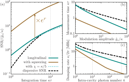
Both expressions have a similar structure, making very clear the similar role of $\tilde{g}_{\mathrm{z}}$ and $\epsilon$, except for the cosine that is a signature of the complex path in phase space of the dispersive case. Importantly, for short measurement times $\kappa\tau\ll 1$, we find a favorable scaling for longitudinal readout with $\mathrm{SNR}_{\mathrm{z}}\propto\mathrm{SNR}_{\chi}/\kappa\tau$. This advantage is illustrated in Fig. 2(a) that shows the SNR versus integration time for longitudinal (full green line) and dispersive (dashed black line) coupling. At equivalent steady-state separation ($\tilde{g}_{\mathrm{z}}=\epsilon$), this leads to shorter measurement time for longitudinal coupling. This is made clear in Fig. 2(b) presenting the measurement time required to reach a fidelity of $99.99\%$ as a function of the modulation amplitude.

As evidenced by the above discussion, for $\tilde{g}_{\mathrm{z}}=\epsilon$ the advantage over dispersive readout is found at short integration times. This is especially true when considering the non-perturbative effects that affect the QNDness of dispersive readout. As an illustration of this, Fig. 2(c) shows the cavity damping rate vs photon number required to reach a fidelity of 99.99% in the short measurement time $\tau=50$ ns. The full green line again represents longitudinal readout and the dashed black line the dispersive case. The horizontal dotted line at $\kappa/2\pi=4$ MHz is a typical value for circuit QED experiments and in particular corresponds to Ref. Jeffrey et al. (2014) where a fidelity of 99.8% was achieved in 140 ns. With this $\kappa$, reaching a fidelity of 99.99% in 50 ns with dispersive readout would require as many as 500 photons (see vertical dotted line). For most circuit QED experiments, this is well above $n_{\mathrm{crit}}$ where non-perturbative effects are expected to reduce the readout fidelity. On the other hand, reaching the same goal with longitudinal readout only requires $\sim 40$ photons. Importantly, working at larger photon number is also a possibility here since there is no critical photon number. Alternatively, working with $\sim 10$ photons requires a large cavity damping rate $\kappa/2\pi\sim 10$ MHz to reach the above goal. Under transverse coupling, this would lead to significant Purcell decay. Indeed, for the typical value $g_{\mathrm{x}}/\Delta\sim 1/10$, the cavity-induced relaxation time $1/\gamma_{\kappa}\sim 1.6~{}\mu$s is much smaller than current qubit relaxation times. As already mentioned above, longitudinal coupling does not lead to Purcell decay Kerman (2013); Billangeon et al. (2015).

In short, the proposed approach allows to reach large readout fidelities in short measurement times. Reaching the same goal with dispersive readout requires either large $\kappa$ or large $\bar{n}$, something that in practice would lead to a reduction of the readout fidelity. It is also interesting to point out that longitudinal readout saturates the inequality $\Gamma_{\varphi\mathrm{m}}\geq\Gamma_{\mathrm{meas}}$ linking the measurement-induced dephasing rate $\Gamma_{\varphi\mathrm{m}}$ to the measurement rate $\Gamma_{\mathrm{meas}}$ and is therefore quantum limited SM .

Single-mode squeezing – The SNR of longitudinal readout can also be exponentially improved with a single-mode squeezed input state on the cavity. For this it suffices to chose the squeeze axis to be orthogonal to the qubit-state dependent displacement generated by $g_{\mathrm{z}}(t)$. In Fig. 1(a), this corresponds to orienting the squeeze axis along the vertical axis. With this choice, and since the squeeze angle is unchanged under evolution with longitudinal coupling, the imprecision noise is exponentially reduced and the signal-to-noise ratio simply becomes $e^{r}\mathrm{SNR}_{\mathrm{z}}$, with $r$ the squeeze parameter SM . This exponential enhancement is apparent from the full brown line in Fig. 2(a) and in the corresponding reduction of the measurement time in Fig. 2(b).

This is in stark contrast to standard dispersive readout where single-mode squeezing can lead to an increase of the measurement time Barzanjeh et al. (2014); Didier et al. (2015). Indeed, under dispersive coupling, the squeeze angle undergoes a qubit-state dependent rotation. As a result, both the squeezed and the anti-squeezed quadrature contributes to the imprecision noise. We note that the situation can be different in the presence of two-mode squeezing Barzanjeh et al. (2014) where the present exponential increase in SNR can be recovered by engineering the dispersive coupling of the qubit to two cavities Didier et al. (2015).

Figure 3: (a) Circuit QED implementation of longitudinal coupling with a transmon qubit of Josephson energies $E_{J1}=E_{J}(1+d)/2$, $E_{J2}=E_{J}(1-d)/2$ with $d\in[0,1]$. (b) $g_{\mathrm{z}}$ and $g_{\mathrm{x}}$ versus flux. Around $\Phi_{\mathrm{x}}=0$, $g_{\mathrm{z}}$ as a linear dependence with flux. The spurious transverse coupling $g_{\mathrm{x}}$ results from qubit asymmetry, here $d=0.02$. The dashed lines represent the asymptotic expressions Eqs. (5) and (6), the full lines to exact numerical result SM . (c) Transmon frequency versus flux for $E_{J}/h=20$ GHz, $E_{J}/E_{C}=67$ and $d=0.02$.

Circuit QED implementation – We now turn to a possible realization of this protocol in circuit QED. Longitudinal coupling of a flux or a transmon qubit to a LC oscillator was already discussed in Refs. Kerman (2013); Billangeon et al. (2015). There, longitudinal coupling results from the mutual inductive coupling between a flux-tunable qubit and the oscillator. As another example, we follow the general approach developed in Ref. Bourassa et al. (2009) and focus on a transmon qubit that is phase-biased by the oscillator. Fig. 3(a) schematically represents a lumped version of this circuit. In practice, the inductors can be replaced by a junction array Manucharyan et al. (2009), both to increase the coupling and to reduce the size of the qubit’s flux-bias loop. An in-depth analysis of an alternative realization based on a transmission-line resonator can be found in Ref. SM .

The Hamiltonian of the circuit of Fig. 3(a) is similar to that of a flux-tunable transmon, but where the external flux $\Phi_{\mathrm{x}}$ is replaced by $\Phi_{\mathrm{x}}+\delta$ with $\delta$ the phase drop at the oscillator Vion et al. (2002). Taking the junction capacitances to be equal and assuming for simplicity that $Z_{0}/R_{K}\ll 1$ with $Z_{0}=\sqrt{L/C}$ and $R_{K}$ the resistance quantum, this Hamiltonian can be expressed as $\hat{H}=\hat{H}_{\mathrm{r}}+\hat{H}_{\mathrm{q}}+\hat{H}_{\mathrm{qr}}$. In this expression, $\hat{H}_{\mathrm{r}}=\omega_{\mathrm{r}}\hat{a}^{\dagger}\hat{a}$ is the oscillator Hamiltonian and $\hat{H}_{\mathrm{q}}=\omega_{\mathrm{a}}\hat{\sigma}_{z}/2$ is the Hamiltonian of a flux-tunable transmon that we write here in its two-level approximation Koch et al. (2007). The qubit-oscillator interaction takes the form $\hat{H}_{\mathrm{qr}}=g_{\mathrm{x}}(\hat{a}^{\dagger}+\hat{a})\hat{\sigma}_{x}+g_{z}(\hat{a}^{\dagger}+\hat{a})\hat{\sigma}_{z}$ with SM

$$g_{\mathrm{z}} =-\frac{E_{J}}{2}\left(\frac{2E_{C}}{E_{J}}\right)^{1/2}\sqrt{\frac{\pi Z_{0}}{R_{K}}}\sin\left(\frac{\pi\Phi_{\mathrm{x}}}{\Phi_{0}}\right),$$ (5)

$$g_{\mathrm{x}} =dE_{J}\left(\frac{2E_{C}}{E_{J}}\right)^{1/4}\sqrt{\frac{\pi Z_{0}}{R_{K}}}\cos\left(\frac{\pi\Phi_{\mathrm{x}}}{\Phi_{0}}\right),$$ (6)

and where $E_{J}$ is the mean Josephson energy, $d$ the Josephson energy asymmetry and $E_{C}$ the qubit’s charging energy. Expressions for these quantities in terms of the elementary circuit parameters are given in Ref. SM . As desired, the transverse coupling $g_{\mathrm{x}}$ vanishes exactly for a symmetric transmon with $d=0$, leaving only longitudinal coupling $g_{\mathrm{z}}$. Thanks to the phase bias rather than inductive coupling, $g_{\mathrm{z}}$ can be made large Bourassa et al. (2009). For example, with the realistic values $E_{J}/h=20$ GHz, $E_{J}/E_{C}=67$ and $Z_{0}=50~{}\Omega$ we find $g_{\mathrm{z}}/2\pi\approx 135~{}\mathrm{MHz}\times\sin\left(\pi\Phi_{\mathrm{x}}/\Phi_{0}\right)$. The flux dependence of both $g_{\mathrm{z}}$ (blue lines) and $g_{\mathrm{x}}$ (red lines) for a finite asymmetry $d=0.02$ are illustrated in Fig. 3(b). The dashed lines refer to the above asymptotic expressions for $g_{\mathrm{z}}$ and $g_{\mathrm{x}}$ while the full lines are exact numerical results. Modulating the flux by $0.05\Phi_{0}$ around $\Phi_{\mathrm{x}}=0$, we find $\tilde{g}_{\mathrm{z}}/2\pi\sim 21$ MHz. This is accompanied by a small change of the qubit frequency of $\sim 40$ MHz, see Fig. 3(c). Importantly, this frequency change does not affect the SNR under longitudinal readout SM .

Tolerance to imperfections – When $d\neq 0$, a finite transversal coupling is present. This is illustrated in Fig. 3(b) where for a realistic value of $d=0.02$ Fink et al. (2009) and the above parameters we find $g_{\mathrm{x}}/2\pi\approx 13~{}\mathrm{MHz}\times\cos\left(\pi\Phi_{\mathrm{x}}/\Phi_{0}\right)$. The effect of this unwanted coupling can be mitigated by working at large qubit-resonator detuning $\Delta$ where the resulting dispersive interaction $\chi=g_{\mathrm{x}}^{2}/\Delta$ can be made small. For exemple, the above numbers correspond to a detuning of $\Delta/2\pi=3$ GHz where $\chi/2\pi\sim 5.6$ kHz. It is important to emphasize that, contrary to dispersive readout, the longitudinal approach is not negatively affected by a large detuning. The large detuning moreover reduces Purcell decay which, for the above $g_{\mathrm{x}}$, can very easily be made small enough to avoid the qubit from being Purcell limited.

When considering higher-order terms in $Z_{0}/R_{K}$, the Hamiltonian of the circuit of Fig. 3(a) contains a dispersive-like interaction $\chi_{\mathrm{z}}\hat{a}^{\dagger}\hat{a}\hat{\sigma}_{z}$ even at $d=0$. For the parameters already used above, we find $\chi_{\mathrm{z}}/2\pi\sim$ 5.3 MHz SM . Contrary to the standard dispersive coupling, $\chi_{\mathrm{z}}$ cannot be made small by detuning the qubit from the resonator. However since it is not derived from a transverse coupling, it is not linked to any Purcell decay. Moreover, at small integration times $\mathrm{SNR}_{\mathrm{z}}$ is not affected by a finite dispersive-like coupling SM . This is illustrated in Fig. 2(a) where the cyan dotted line, corresponding $\mathrm{SNR}_{\mathrm{z}}$ in the presence of $\chi=\kappa/5$, is barely distinguishable from the ideal case.

Finally, when discussing the exponential gain in SNR provided by single-mode squeezing, we have assumed a source of broadband pure squeezing. The effect of a finite squeezing bandwidth $\Gamma$ was already studied in Ref. Didier et al. (2015) and only leads to a small reduction of the SNR for $\Gamma\gg\kappa$. On the other hand, deviation from unity of the squeezing purity $P$ leads to a reduction of the SNR by $1/\sqrt{P}$. The SNR being decoupled from the anti-squeezed quadrature, the purity simply renormalizes the squeeze parameter.

Multi-qubit architecture – A possible mutli-qubit architecture consists of qubits longitudinally coupled to a readout resonator (of annihilation operator $\hat{a}_{\mathrm{z}}$) and transversally coupled to a high-Q bus resonator ($\hat{a}_{\mathrm{x}}$). The Hamiltonian describing this system is

$$\begin{split}\hat{H}&=\omega_{\mathrm{rz}}\hat{a}_{\mathrm{z}}^{\dagger}\hat{a}_{\mathrm{z}}+\omega_{\mathrm{rx}}\hat{a}_{\mathrm{x}}^{\dagger}\hat{a}_{\mathrm{x}}+\sum_{j}\tfrac{1}{2}\omega_{\mathrm{a}j}\hat{\sigma}_{zj}\\ &+\sum_{j}g_{\mathrm{z}j}\hat{\sigma}_{zj}(\hat{a}_{\mathrm{z}}^{\dagger}+\hat{a}_{\mathrm{z}})+\sum_{j}g_{\mathrm{x}j}\hat{\sigma}_{xj}(\hat{a}_{\mathrm{x}}^{\dagger}+\hat{a}_{\mathrm{x}}).\end{split}$$ (7)

In this architecture, readout is realized by taking advantage of the longitudinal coupling while logical operation are realized using the bus resonator. A scalable architecture taking advantage of longitudinal coupling is discussed at length in Ref. Billangeon et al. (2015). Here, we again consider that the longitudinal coupling of each qubit can be modulated independently. We take this modulation to be $g_{\mathrm{z}j}(t)=\bar{g}_{\mathrm{z}}+\tilde{g}_{\mathrm{z}}\cos(\omega_{\mathrm{r}}t+\varphi_{j})$ where the phase $\varphi_{j}$ is adjustable. In the interaction picture and neglecting fast-oscillating terms, the longitudinal coupling becomes

$$\tilde{H}_{\mathrm{z}}=\Big{(}\tfrac{1}{2}\tilde{g}_{\mathrm{z}}\sum_{j}\hat{\sigma}_{zj}e^{-i\varphi_{j}}\Big{)}\hat{a}_{\mathrm{z}}+\mathrm{h.c.}$$ (8)

This effective drive on the resonator displaces the field to a multi-qubit-state dependent coherent state allowing single-shot multi-qubit measurements. For two qubits, $\varphi_{j}=j\pi/2$ leads to four well separated states in phase space. Other choices of phase lead to overlapping pointer states corresponding to different multi-qubit states. Exemples are $\varphi_{j}=0$ for which the two-qubit states $|01\rangle$ and $|10\rangle$ are indistinguishable, and $\varphi_{j}=j\pi$ where these states are replaced by $|00\rangle$ and $|11\rangle$. This can be exploited to create entanglement by measurement Lalumière et al. (2010). The 3-qubit GHZ state is obtained with $\varphi_{j}=j2\pi/3$ SM .

Conclusion– We have shown that modulating longitudinal coupling between a qubit and an oscillator leads to fast QND qubit readout. Because of the optimal motion of the pointer states in phase, the measurement time is reduced with respect to standard dispersive readout. For the same reason, this approach can be further improved by using single-mode squeezing.

Acknowledgements– We thank A. Clerk for useful discussions. This work was supported by the Army Research Office under Grant W911NF-14-1-0078, INTRIQ and NSERC.

See pages 1 of longitudinal_SM See pages 2 of longitudinal_SM See pages 3 of longitudinal_SM See pages 4 of longitudinal_SM See pages 5 of longitudinal_SM See pages 6 of longitudinal_SM See pages 7 of longitudinal_SM See pages 8 of longitudinal_SM See pages 9 of longitudinal_SM

References

- Haroche and Raimond (2006) S. Haroche and J.-M. Raimond, Exploring the Quantum: Atoms, Cavities, and Photons (Oxford University Press, Oxford, 2006).
- Castellanos-Beltran et al. (2008) M. A. Castellanos-Beltran, K. D. Irwin, G. C. Hilton, L. R. Vale, and K. W. Lehnert, Nature Phys. 4, 929 (2008).
- Bergeal et al. (2010) N. Bergeal, F. Schackert, M. Metcalfe, R. Vijay, V. E. Manucharyan, L. Frunzio, D. E. Prober, R. J. Schoelkopf, S. M. Girvin, and M. H. Devoret, Nature 465, 64 (2010).
- Eichler and Wallraff (2014) C. Eichler and A. Wallraff, EPJ Quantum Technology 1, 2 (2014).
- Vijay et al. (2011) R. Vijay, D. H. Slichter, and I. Siddiqi, Phys. Rev. Lett. 106, 110502 (2011).
- Vijay et al. (2012) R. Vijay, C. Macklin, D. H. Slichter, S. J. Weber, K. W. Murch, R. Naik, A. N. Korotkov, and I. Siddiqi, Nature 490, 77 (2012).
- Hatridge et al. (2013) M. Hatridge, S. Shankar, M. Mirrahimi, F. Schackert, K. Geerlings, T. Brecht, K. M. Sliwa, B. Abdo, L. Frunzio, S. M. Girvin, R. J. Schoelkopf, and M. H. Devoret, Science 339, 178 (2013).
- Jeffrey et al. (2014) E. Jeffrey, D. Sank, J. Y. Mutus, T. C. White, J. Kelly, R. Barends, Y. Chen, Z. Chen, B. Chiaro, A. Dunsworth, A. Megrant, P. J. J. O’Malley, C. Neill, P. Roushan, A. Vainsencher, J. Wenner, A. N. Cleland, and J. M. Martinis, Phys. Rev. Lett. 112, 190504 (2014).
- Raussendorf and Harrington (2007) R. Raussendorf and J. Harrington, Phys. Rev. Lett. 98, 190504 (2007).
- Houck et al. (2008) A. A. Houck, J. A. Schreier, B. R. Johnson, J. M. Chow, J. Koch, J. M. Gambetta, D. I. Schuster, L. Frunzio, M. H. Devoret, S. M. Girvin, and R. J. Schoelkopf, Phys. Rev. Lett. 101, 080502 (2008).
- Boissonneault et al. (2009) M. Boissonneault, J. Gambetta, and A. Blais, Phys. Rev. A 79, 013819 (2009).
- Slichter et al. (2012) D. H. Slichter, R. Vijay, S. J. Weber, S. Boutin, M. Boissonneault, J. M. Gambetta, A. Blais, and I. Siddiqi, Phys. Rev. Lett. 109, 153601 (2012).
- Blais et al. (2004) A. Blais, R.-S. Huang, A. Wallraff, S. Girvin, and R. Schoelkopf, Phys. Rev. A 69, 062320 (2004).
- Kerman (2013) A. J. Kerman, New Journal of Physics 15, 123011 (2013).
- Billangeon et al. (2015) P.-M. Billangeon, J. S. Tsai, and Y. Nakamura, Phys. Rev. B 91, 094517 (2015).
- Barzanjeh et al. (2014) S. Barzanjeh, D. P. DiVincenzo, and B. M. Terhal, Phys. Rev. B 90, 134515 (2014).
- Didier et al. (2015) N. Didier, A. Kamal, A. Blais, and A. A. Clerk, ArXiv e-prints (2015), arXiv:1502.00607 [quant-ph] .
- Koch et al. (2007) J. Koch, T. Yu, J. Gambetta, A. Houck, D. Schuster, J. Majer, A. Blais, M. Devoret, S. Girvin, and R. Schoelkopf, Phys. Rev. A 76, 042319 (2007).
- Milburn et al. (2000) G. Milburn, S. Schneider, and D. James, Fortschritte der Physik 48, 801 (2000).
- Sørensen and Mølmer (2000) A. Sørensen and K. Mølmer, Phys. Rev. A 62, 022311 (2000).
- Garcia-Ripoll et al. (2003) J. J. Garcia-Ripoll, P. Zoller, and J. I. Cirac, Phys. Rev. Lett. 91, 157901 (2003).
- Leibfried et al. (2003) D. Leibfried, B. DeMarco, V. Meyer, D. Lucas, M. Barrett, J. Britton, W. M. Itano, B. Jelenkovic, C. Langer, T. Rosenband, and D. J. Wineland, Nature 422, 412 (2003).
- Blais et al. (2007) A. Blais, J. Gambetta, A. Wallraff, D. I. Schuster, S. M. Girvin, M. H. Devoret, and R. J. Schoelkopf, Physical Review A (Atomic, Molecular, and Optical Physics) 75, 032329 (2007).
- (24) See Supplemental Material for more information.
- Gambetta et al. (2008) J. Gambetta, A. Blais, M. Boissonneault, A. A. Houck, D. I. Schuster, and S. M. Girvin, Phys. Rev. A 77, 012112 (2008).
- Bourassa et al. (2009) J. Bourassa, J. M. Gambetta, J. A. A. Abdumalikov, O. Astafiev, Y. Nakamura, and A. Blais, Phys. Rev. A 80, 032109 (2009).
- Manucharyan et al. (2009) V. E. Manucharyan, J. Koch, L. I. Glazman, and M. H. Devoret, Science 326, 113 (2009).
- Vion et al. (2002) D. Vion, A. Aassime, A. Cottet, P. Joyez, H. Pothier, C. Urbina, D. Esteve, and M. Devoret, Science 296, 886 (2002).
- Fink et al. (2009) J. M. Fink, R. Bianchetti, M. Baur, M. Göppl, L. Steffen, S. Filipp, P. J. Leek, A. Blais, and A. Wallraff, Phys. Rev. Lett. 103, 083601 (2009).
- Lalumière et al. (2010) K. Lalumière, J. M. Gambetta, and A. Blais, Phys. Rev. A 81, 040301 (2010).