Numerical approximation of positive power curvature flow via deterministic games.

Abstract

We approximate the level set solution for the motion of an embedded closed curve in the plane with normal speed $\max(0,\kappa)^{\gamma}$ where $\kappa$ is the curvature of the curve and $\frac{1}{3}<\gamma<1$ by the value functions of a family of deterministic two person games. We show convergence of the value functions to the viscosity solution of the level set equation and propose a numerical scheme for the calculation of the value function. We illustrate the convergence properties of the scheme for different parameter values in some example cases.

mmsxxxxxxxx–x

1 Introduction

In [24] R. Kohn and S. Serfaty present a game theoretic approach to the curve-shortening flow, i.e. the mean curvature flow of curves in the plane. The (time-dependent) level set formulation of this flow is a degenerate parabolic, possibly singular equation and is interpreted as the limit of the value functions of a family of discrete-time, two-person games. It is proved that these value functions converge to the viscosity solution of the level set equation, cf. [24, Theorem 2]. Furthermore, using a ’minimal exit time game’ a rate for the convergence of the value functions of this game to the time-independent level set formulation of the (mean) curvature flow is proved in [24]. We note, that the corresponding convergence result (without rates) for the positive curvature flow (here the normal speed is the curvature if it is nonnegative and zero otherwise) is given in [24, Theorem 5]. In contrast to the curve shortening flow not much is known about the behavior of a non convex initial curve in the plane moving by positive curvature flow. But the latter has been used for image processing, see the remarks in [24, page 16] and [29]. In form of examples modified flows are presented in [24, Section 1.7] which have a game theoretic interpretation. But proofs of convergence for the value functions of the corresponding games for these modified examples are not given therein. Among these is a game, cf. [24, Example 3, Section 1.7], which can handle the case of the curvature flow of a convex curve in the plane at which the normal speed is given – instead of the curvature – by a power $\gamma>0$ of the (mean) curvature. We call this power curvature flow (PCF) (and the analogous flow for hypersurfaces power mean curvature flow (PMCF)). PCF is only a well-defined flow when the initial curve is convex. In [24] five open questions are formulated, cf. [24, Section 1.8]; among these is the question of numerical advantages or disadvantages of this approach.

In this paper we consider for $\frac{1}{3}<\gamma<1$ the more general, so-called positive power curvature flow PPCF for which the normal speed is given by $\kappa_{+}^{\gamma}$ (where $\kappa_{+}=\max(0,\kappa)$) and which coincides with PCF if the initial curve is convex. Our aim is to approximate this flow by a family of value functions of suitable games. We show convergence of the value functions to the unique viscosity solution of the time-dependent level set formulation of PPCF and present a numerical algorithm for this approach. We demonstrate the convergence of the algorithm for some example cases and analyze the effect of different choices for the numerical parameters.

Let us relate the content of our paper to [24]. There is no game in [24] for PPCF. The game in [24, Example 3, Section 1.7] is suggested therein to approximate PCF in case $0<\gamma<1$. The corresponding limit equation [24, (1.23)] has the (formal) disadvantage that its left-hand side becomes $-\infty$ if there are non convex zero-level sets (in case they are curves) of the continuum solution (e.g. at the initial time outside of the initial curve). By considering PPCF we avoid this convexity issue, especially we can use non convex initial curves. The game we use for the approximation of PPCF is essentially the one in [24, Example 3, Section 1.7] but it turns out that it is necessary (at least for our proof) to use a slightly different definition of the value function. The difference is that we take the minimum in the definition of the value function over a ($\epsilon$-dependent) compact subinterval of $(0,\infty)$ instead over $(0,\infty)$, cf. (9). This difference is not due to the fact that we consider PPCF instead of PCF but is of general nature. The initial and endpoints of the subintervals $I_{\epsilon}$ have to satisfy some technical relations, cf. (10)-(12), which imply that we need the restriction $\frac{1}{3}<\gamma<1$. The interesting point is that $\frac{1}{3}$ is exactly the critical value at which the convergence behavior of PCF changes, see Theorem 2 and the following remarks.

Concerning a numerical application of the Kohn-Serfaty approach to the curve shortening flow (i.e. $\gamma=1$) we refer to [11]. In addition therein a semi-Lagrangian approximation of the curve shortening flow is considered. A semi-Lagrangian approach for the affine curvature flow case which corresponds to $\gamma=\frac{1}{3}$ is content of [12].

We give some references for the numerical approximation of flows by powers of the curvature (which do not use the Kohn-Serfaty approach). A numerical approximation of the stationary level set solution of PCF in case $\gamma\geq 1$ is content of our two previous papers [26] and [27]. There we approximate the regularized stationary level set equation (used in [36] to prove existence of the stationary level set PMCF) by finite elements and prove rates for the approximation errors. The stationary level set equation of mean curvature flow is also content of [10].

There are only few numerical papers which deal with PCF for $\gamma\neq 1$.

In [7] and [8] stability bounds for a finite element approximation of PCF for curves is derived, see also [9]. In [30] the parametric formulation of the evolution of plane curves driven by a nonlinear function of curvature and anisotropy is considered. Concerning PCF from the perspective of image processing we refer to [1] [2], [34], [28] and [29].

For estimates of the regularization error for the instationary level set formulation of mean curvature flow we refer to [31] and [17]. For more general references to the numerical treatment of motion by curvature we refer to [31], [19], [17], [32], [18] , [20], [33] and [40] where the instationary level set formulation is considered.

Our paper is organized as follows. In the remaining part of the present section we formulate some known results about the behavior of curves evolving under PCF. In Section 2 we define the value functions $u^{\epsilon}$. In Section 3 we show convergence of the value functions to the solution of the continuous problem. In Section 4 we present the algorithm in order to calculate $u^{\epsilon}$. Its application in some example cases as well as the effect of the choice of different numerical parameters is content of Section 5.

As for the positive curvature flow little is known about the behavior of PPCF for not convex initial curves. We state some well-known facts about the behavior of curves evolving under PCF in case $0<\gamma\leq 1$, see [4] and [3], and remark that in these references also the case $\gamma>1$ is treated.

Theorem 1.

Let $\gamma=1$ and $\Gamma_{0}$ a smooth, embedded closed curve given by an embedding $x_{0}:S^{1}\rightarrow\mathbb{R}^{2}$. Then there exists a unique smooth solution $x:S^{1}\times[0,T)\rightarrow\mathbb{R}^{2}$ of

(1) $$\frac{d}{dt}x=-\kappa^{\gamma}\nu\quad(=-\kappa\nu)$$

where $\nu$ denotes the outer unit normal, with initial data $x_{0}$. $\Gamma_{t}=x(S^{1},t)$ converges to a point $p\in\mathbb{R}^{2}$ as $t\rightarrow T$. The rescaled curves $(\Gamma_{t}-p)/\sqrt{2(T-t)}$ converge to the unit circle about the origin as $t\rightarrow T$.

The assumption of smoothness of the initial curve in Theorem 1 can be relaxed to allow $\Gamma_{0}$ to be the boundary of a bounded open convex region and the curves $\Gamma_{t}$ are converging to $\Gamma_{0}$ in Hausdorff distance as $t\rightarrow 0$, see [5].

If $\gamma=\frac{1}{3}$ and $\Gamma_{0}$ a smooth, convex, embedded closed curve then Theorem 1 still holds with a different rescaling, namely $(\Gamma_{t}-p)/(4(T-t)/3)^{\frac{3}{4}}$ converges to an ellipse of enclosed area $\pi$ centered at the origin. The regularity assumption on the initial curve can be weakened to allow boundaries of open bounded convex regions. For $\gamma\in[\frac{1}{3},1]$ we get the following result.

Theorem 2.

If $\gamma\in[\frac{1}{3},1]$ and $\Gamma_{0}$ the boundary curve of an open bounded convex set in $\mathbb{R}^{2}$ then (1) has a smooth and strictly convex solution for $0<t<T$ which converges to a point $p\in\mathbb{R}^{2}$ and the rescaled curves $(\Gamma_{t}-p)/(T-t)^{\frac{1}{1+\gamma}}$ converge smoothly to a limit curve $\Gamma_{\gamma}$ which satisfies $\kappa^{\gamma}=\lambda\left<x,\nu\right>$ for some $\lambda>0$.

Curves $\Gamma_{\lambda}$ are called homothetic solutions and in case $\gamma>\frac{1}{3}$ all homothetic solutions are circles. For $\gamma=\frac{1}{3}$ the only homothetic solutions are ellipses. For $0<\gamma<\frac{1}{3}$ a classification of homothetic solutions is given in [4, Theorem 1.5].

There are results for non-convex initial curves in [6] and [15, Chapter 8].

For $0<\gamma<\frac{1}{3}$ the isoperimetrical ratio becomes unbounded near the final time for generic symmetric initial data, cf. the remarks in [4, Section 1].

There are results on PMCF in case of $n$-dimensional hypersurfaces in Euclidean space, $n\geq 2$, see for example [35] and [37] for the parametric formulation and [36] for the time-independent level set formulation in case $\gamma\geq 1$ and [31] (and references therein) for the time-dependent level set formulation of PCF in case $0<\gamma\leq 1$.

Concerning a time-dependent level set equation for PCF we only know the equation

(2) $$u_{t}= |Du|\left\{\operatorname{div}\left(\frac{Du}{|Du|}\right)\right\}^{\gamma}$$

$$= \left\{\sum_{i,j}\left(\delta_{ij}-\frac{D_{i}uD_{j}u}{|Du|^{2}}\right)D_{i}D_{j}u\right\}^{\gamma}|Du|^{1-\gamma}$$

in case $\gamma=\frac{1}{2n-1}$, $n\in\mathbb{N}$, which is a little bit different from PCF since here negative curvatures are allowed. For PPCF the time-dependent level set equation is given by

(3) $$u_{t}= |Du|\left\{\operatorname{div}\left(\frac{Du}{|Du|}\right)\right\}_{+}^{\gamma}$$

$$= \left\{\sum_{i,j}\left(\delta_{ij}-\frac{D_{i}uD_{j}u}{|Du|^{2}}\right)D_{i}D_{j}u\right\}_{+}^{\gamma}|Du|^{1-\gamma}$$

for general $0<\gamma\leq 1$. We consider these equations in $\mathbb{R}^{2}\times(0,\infty)$ with initial condition $u(\cdot,0)=u_{0}$. We assume that $u_{0}\in C^{0,1}(\mathbb{R}^{2})$, $|u_{0}|\leq 1$ and $u_{0}(x)=1$ for $x\in\mathbb{R}^{2}\backslash B_{R}(0)$ where $R>0$ is a sufficiently large radius.

Equations (2), (3) are fundamental equations in image processing, especially in the case $\gamma=\frac{1}{3}$ where these equations are the so-called affine curvature equations, cf. [1] and [22]. Equations (2), (3) are included by the general geometric equations which are dealt in [14], [23] and [22] and therefore for each equation exists a unique viscosity solution. We mention [31] where convergence with rates of a regularization of (2) is proved.

2 Game theoretic interpretation and definition of $u^{\epsilon}$

Let $\Omega$ be a smooth, bounded domain in the plane and $T>0$. Let $u_{0}$ be a Lipschitz continuous function in the plane with $u_{0}<0$ in $\Omega$, $u_{0}\geq 0$ in $\mathbb{R}^{2}\backslash\bar{\Omega}$ and $|u_{0}|\leq 1$. We assume $\frac{1}{3}<\gamma<1$ and consider the following continuum equation

(4) $$\begin{cases}u_{t}-|\nabla u|\varphi(\operatorname{curv}(u))&=0\\ u(\cdot,T)&=u_{0}\end{cases}$$

where

(5) $$\operatorname{curv}(u)=-\operatorname{div}(\nabla u/|\nabla u|)$$

is the curvature of the level set and

(6) $$\varphi(\kappa)=\begin{cases}-|\kappa|^{\gamma},\quad&\kappa\leq 0\\ 0,\quad&\kappa>0.\end{cases}$$

We note, that in this sense the curvature of the unit circle is $-1$ because in $\{x\in\mathbb{R}^{n+1}:|x|-1=0\}$ we have $\operatorname{curv}(|x|)=-\operatorname{div}\left(\frac{x}{|x|}\right)=-n<0$ in view of (5). Furthermore, (4) is not PPCF but after transforming the time variable $t\mapsto T-t$ we get the correct equation, i.e. PPCF (3). As already explained above our equation (4) differs from the continuum equation in [24, Section 1.7, Example 3] in the fact that the latter requires $u_{t}=\infty$ if $\operatorname{curv}(u)>0$.

The goal is to approximate (4) by the value functions of certain deterministic, time-discrete two person games. For the convergence proof it will be crucial that for $\kappa\leq 0$ we can write

(7) $$\varphi(\kappa)=\sup_{s>0}\left(\frac{1}{2}\kappa s^{2}-f(s)\right)$$

where

(8) $$f(s)=c_{\gamma}s^{\frac{2\gamma}{\gamma-1}},\quad c_{\gamma}=(1-\gamma)(2\gamma)^{\frac{\gamma}{1-\gamma}}.$$

The value functions $u^{\epsilon}$, $\epsilon>0$, are defined for $x\in\Omega$ and $0\leq t\leq T$ by

(9) $$u^{\epsilon}(x,t)=\min_{\|v\|=1,s\in I_{\epsilon}}\max_{b,\beta\in\{-1,1\}}u^{\epsilon}(x+b\epsilon sv+\beta\epsilon^{2}f(s)v^{\perp},t+\epsilon^{2})$$

where

(10) $$I_{\epsilon}=[\epsilon^{\alpha_{1}},\epsilon^{-\alpha_{2}}]$$

with

(11) $$\frac{1-\gamma}{2\gamma}<\alpha_{1}<\min\left(1,\frac{1-\gamma}{\gamma}\right)$$

and

(12) $$0<\alpha_{2}<\min\left(\alpha_{1}\frac{2\gamma}{1-\gamma}-1,\frac{1}{3}\right).$$

The difference from our definition to the definition in [24, Example 3, Section 1.7] is that we minimize over $s\in I_{\epsilon}$ instead of $s>0$. The first inequality in (11) implies that the RHS of (12) is positive so that there exists a corresponding $\alpha_{2}$. The $\alpha_{1}<1$ part of the second inequality in (11) is needed for Case (1) in part (ii) of the proof of Lemma 5. The other part of the second inequality in (11) implies that the step size is at most a fixed positive power of $\epsilon$. The first part of the second inequality in (12) is needed for part (i) of the proof of Lemma 5 while the second part is used for Case (2ba) of part (ii) of the proof of Lemma 5. Inequality (11) implies $\gamma>\frac{1}{3}$ which is the reason why we have only a convergence result for this case.

We can calculate $u^{\epsilon}$ numerically by setting $u^{\epsilon}(\cdot,T)=u_{0}$ and ’playing the game backwards in time’, i.e. we calculate $u^{\epsilon}(\cdot,T-\epsilon^{2})$, etc..

3 Convergence of the value functions

In this section we show that the value functions converge to a solution of (4). For completeness we give the following definition.

Definition 3.

(i) A lower semicontinuous function $u$ is a viscosity supersolution of (4) if whenever $\phi(x,t)$ is smooth and $u-\phi$ has a local minimum at $(x_{0},t_{0})$ we have

(13) $$\phi_{t}-|\nabla\phi|\varphi(\operatorname{curv}(\phi))\leq 0$$

at $(x_{0},t_{0})$ if $\nabla\phi(x_{0},t_{0})\neq 0$, and

(14) $$\phi_{t}\leq 0$$

at $(x_{0},t_{0})$ if $\nabla\phi(x_{0},t_{0})=0$.

(ii) An upper semicontinuous function $u$ is a viscosity subsolution of (4) if whenever $\phi(x,t)$ is smooth and $u-\phi$ has a local maximum at $(x_{0},t_{0})$ we have

(15) $$\phi_{t}-|\nabla\phi|\varphi(\operatorname{curv}(\phi))\geq 0$$

at $(x_{0},t_{0})$ if $\nabla\phi(x_{0},t_{0})\neq 0$, and

(16) $$\phi_{t}\geq 0$$

at $(x_{0},t_{0})$ if $\nabla\phi(x_{0},t_{0})=0$.

We define

(17) $$\bar{u}(X)= \limsup_{Y\rightarrow X,\epsilon\rightarrow 0}u^{\epsilon}(Y)$$

$$\underline{u}(X)= \liminf_{Y\rightarrow X,\epsilon\rightarrow 0}u^{\epsilon}(Y).$$

$\bar{u}$ is upper semicontinuous, $\underline{u}$ is lower semicontinuous and $\underline{u}\leq\bar{u}$ We will show that $\bar{u}$ is a viscosity subsolution of (4) and that $\underline{u}$ is a viscosity supersolution of (4). Then from a comparison principle we get that $\bar{u}=\underline{u}$ is a solution and that $u^{\epsilon}\rightarrow u$. The proof strategy starts with an argumentation adapted from [24, Section 4.3] and then we distinguish several cases to handle our flow.

Lemma 4.

$\bar{u}$ is a viscosity subsolution of (4).

Proof.

We argue by contradiction. If not, then there is a smooth $\phi$ such that $(x_{0},t_{0})$ is a local maximum of $\bar{u}-\phi$ with

(18) $$\phi_{t}-|\nabla\phi|\varphi(\operatorname{curv}(\phi))\leq\theta_{0}<0\text{ at }(x_{0},t_{0})$$

if $\nabla\phi(x_{0},t_{0})\neq 0$ or we have $\nabla\phi(x_{0},t_{0})=0$ and

(19) $$\phi_{t}\leq\theta_{0}<0$$

in $(x_{0},t_{0})$. Adding to $\phi$ a nonnegative function whose derivatives at $(x_{0},t_{0})$ are all zero up to second order, we can assume that $(x_{0},t_{0})$ is a strict local maximum of $\bar{u}-\phi$ in a $\delta$-neighborhood of $(x_{0},t_{0})$. Let $(x^{0}_{\epsilon},t^{0}_{\epsilon})\rightarrow(x_{0},t_{0})$ such that $u^{\epsilon}(x^{0}_{\epsilon},t^{0}_{\epsilon})\rightarrow\bar{u}(x_{0},t_{0})$.

(i) Let us consider the case $\nabla\phi(x_{0},t_{0})\neq 0$. We may assume that $\nabla\phi\neq 0$ in the above $\delta$-neighborhood. We construct the following sequence

(20) $$X^{\epsilon}_{0}= (x^{0}_{\epsilon},t^{0}_{\epsilon})$$

$$X^{\epsilon}_{1}= \left(x^{0}_{\epsilon}+b_{0}\epsilon s_{0}\frac{\nabla^{\perp}\phi(X^{\epsilon}_{0})}{|\nabla\phi(X^{\epsilon}_{0})|}+\beta_{0}\epsilon^{2}f(s_{0})\frac{\nabla\phi(X^{\epsilon}_{0})}{|\nabla\phi(X^{\epsilon}_{0})|},t^{0}_{\epsilon}+{\epsilon}^{2}\right)$$

$$X^{\epsilon}_{k+1}= X^{\epsilon}_{k}+\left(b_{k}\epsilon s_{k}\frac{\nabla^{\perp}\phi(X^{\epsilon}_{k})}{|\nabla\phi(X^{\epsilon}_{k})|}+\beta_{k}\epsilon^{2}f(s_{k})\frac{\nabla\phi(X^{\epsilon}_{k})}{|\nabla\phi(X^{\epsilon}_{k})|},{\epsilon}^{2}\right)$$

where the $b_{k}$ and $\beta_{k}$ are maximizing $u^{\epsilon}(X^{\epsilon}_{k+1})$ for given $s_{k}$ and $s_{k}\in I_{\epsilon}$ is chosen as will become clear in the following. Then $u^{\epsilon}(X^{\epsilon}_{k})\leq u^{\epsilon}(X^{\epsilon}_{k+1})$ in view of (9) and hence

(21) $$u^{\epsilon}(X^{\epsilon}_{0})\leq u^{\epsilon}(X^{\epsilon}_{k}).$$

We let $X(s)$ be the continuous path that affinely interpolates between these points i.e. $X(t)=X^{\epsilon}_{k}+(\frac{t-k\epsilon^{2}-t^{0}_{\epsilon}}{\epsilon^{2}})(X^{\epsilon}_{k+1}-X^{\epsilon}_{k})$ for $t^{0}_{\epsilon}+k\epsilon^{2}\leq t\leq t^{0}_{\epsilon}+(k+1)\epsilon^{2}$, and write $(x(t),t)=X(t)$. We have

(22) $$\frac{\partial}{\partial t}\phi(X(t))= \partial_{t}\phi(x(t),t)+\nabla\phi(x(t),t)\cdot d_{t}x(t)$$

$$\frac{\partial}{\partial t}\nabla\phi(x(t),t)= \nabla\phi_{t}(x(t),t)+D^{2}\phi(x(t),t)d_{t}x(t)$$

and since

(23) $$d_{t}x(t)=\frac{b_{k}s_{k}}{\epsilon}\frac{\nabla^{\perp}\phi(X^{\epsilon}_{k})}{|\nabla\phi(X^{\epsilon}_{k})|}+\beta_{k}f(s_{k})\frac{\nabla\phi(X^{\epsilon}_{k})}{|\nabla\phi(X^{\epsilon}_{k})|}$$

is constant we get

(24) $$\frac{\partial^{2}}{\partial t^{2}}\phi(X(t))=\partial_{t}^{2}\phi(X(t))+2\nabla\phi_{t}(X(t))\cdot d_{t}x(t)+\left<D^{2}\phi(X(t))d_{t}x(t),d_{t}x(t)\right>.$$

Taylor expansion of $t\mapsto\phi(X(t))$ at $t^{0}_{\epsilon}+k\epsilon^{2}$ gives

(25) $$\phi(X^{\epsilon}_{k+1})- \phi(X^{\epsilon}_{k})$$

$$= \epsilon^{2}\frac{d}{dt}\phi(X(t^{0}_{\epsilon}+k\epsilon^{2}))+\frac{\epsilon^{4}}{2}\frac{d^{2}}{dt^{2}}\phi(X(t^{0}_{\epsilon}+k\epsilon^{2}))$$

$$= \epsilon^{2}\left(\partial_{t}\phi(X^{\epsilon}_{k})+\nabla\phi(X^{\epsilon}_{k})d_{t}x(t)\right)$$

$$+\frac{\epsilon^{4}}{2}\left(\partial_{t}^{2}\phi(X^{\epsilon}_{k})+2\nabla\phi_{t}(X^{\epsilon}_{k})d_{t}x(t)+\left<D^{2}\phi(X^{\epsilon}_{k})d_{t}x(t),d_{t}x(t)\right>\right)$$

$$+o(\epsilon^{2})$$

$$= \epsilon^{2}\left(\partial_{t}\phi(X^{\epsilon}_{k})+|\nabla\phi(X^{\epsilon}_{k})|\beta_{k}f(s_{k})\right)$$

$$+\frac{\epsilon^{2}}{2}b_{k}^{2}s_{k}^{2}\left<D^{2}\phi(X^{\epsilon}_{k})\frac{\nabla^{\perp}\phi(X^{\epsilon}_{k})}{|\nabla\phi(X^{\epsilon}_{k})|},\frac{\nabla^{\perp}\phi(X^{\epsilon}_{k})}{|\nabla\phi(X^{\epsilon}_{k})|}\right>+o(\epsilon^{2})$$

$$= \epsilon^{2}\left(\partial_{t}\phi(X^{\epsilon}_{k})+|\nabla\phi(X^{\epsilon}_{k})|(\beta_{k}f(s_{k})-\frac{b_{k}^{2}s_{k}^{2}}{2}\operatorname{curv}(\phi)_{|X^{\epsilon}_{k}})\right)+o(\epsilon^{2})$$

in view of

(26) $$-\operatorname{curv}(\phi)|D\phi|=|\nabla\phi|\operatorname{div}\left(\frac{\nabla\phi}{|\nabla\phi|}\right)=\left<D^{2}\phi\frac{\nabla^{\perp}\phi}{|\nabla\phi|},\frac{\nabla^{\perp}\phi}{|\nabla\phi|}\right>.$$

We use the notation

(27) $$\varphi_{s}(\kappa)=\kappa\frac{s^{2}}{2}-f(s)$$

for $\kappa\in\mathbb{R}$ and $s>0$ and we get

(28) $$\phi(X^{\epsilon}_{k+1})-\phi(X^{\epsilon}_{k}) \leq\epsilon^{2}\left\{\partial_{t}\phi(X^{\epsilon}_{k})-|\nabla\phi(X^{\epsilon}_{k})|\varphi_{s_{k}}(\operatorname{curv}(\phi)_{|X^{\epsilon}_{k}})\right\}+o(\epsilon^{2})$$

We want to show by using (18) that

(29) $$\partial_{t}\phi(X^{\epsilon}_{k})-|\nabla\phi(X^{\epsilon}_{k})|\varphi_{s_{k}}(\operatorname{curv}(\phi)_{|X^{\epsilon}_{k}})\leq\frac{\theta_{0}}{2}$$

for small $\epsilon$. Let us assume for a moment that this is already shown then we have

(30) $$\phi(X^{\epsilon}_{k+1})-\phi(X^{\epsilon}_{k}) \leq\epsilon^{2}\frac{\theta_{0}}{2}$$

and hence

(31) $$\phi(X^{\epsilon}_{k})-\phi(X^{\epsilon}_{0})\leq\frac{k}{2}\epsilon^{2}\theta_{0}<0.$$

Adding this inequality to (21) gives

(32) $$u^{\epsilon}(X^{\epsilon}_{0})-\phi(X^{\epsilon}_{0})\leq u^{\epsilon}(X^{\epsilon}_{k})-\phi(X^{\epsilon}_{k})+\frac{k}{2}\epsilon^{2}\theta_{0}.$$

For each $\epsilon$ we consider the finite sequence $(X^{\epsilon}_{k})_{0\leq k\leq k(\epsilon)}$ where $k(\epsilon)$ is as follows. Let

(33) $$U=B_{\delta}(x_{0},t_{0})\backslash B_{\delta_{1}}(x_{0},t_{0}),\quad 0<\delta_{1}<\delta,$$

we may assume that $X^{\epsilon}_{0}\in B_{\delta_{1}}(x_{0},t_{0})$ and that

(34) $$u^{\epsilon}(X^{\epsilon}_{0})-\phi(X^{\epsilon}_{0})\geq\bar{u}(x_{0},t_{0})-\phi(x_{0},t_{0})-\frac{\theta_{0}}{4}.$$

Let

(35) $$k(\epsilon)=\min\{k\in\mathbb{N}:X^{\epsilon}_{k}\in U\}.$$

Note, that $k(\epsilon)$ is well-defined since (32) and (34) imply that the sequence $(X^{\epsilon}_{k})$ leaves $B_{\delta_{1}}(x_{0},t_{0})$ at the latest for $k=[\epsilon^{-2}]$. Hence (for small $\epsilon$ compared to $\delta$) there must be an element $X^{\epsilon}_{k}\in U$.

For a subsequence $X^{\epsilon}_{k(\epsilon)}\rightarrow(x^{\prime},t^{\prime})\neq(x_{0},t_{0})$ and by (32) we get

(36) $$(\bar{u}-\phi)(x_{0},t_{0})\leq(\bar{u}-\phi)(x^{\prime},t^{\prime})$$

in contradiction to the fact that $(x_{0},t_{0})$ is the unique maximum in $B_{\delta}(x_{0},t_{0})$.

We show (29) by distinguishing cases, thereby we assume $\delta$ to be sufficiently small. We set $\kappa_{0}=\operatorname{curv}(\phi)_{|X_{0}}$ and $\kappa_{k}=\operatorname{curv}(\phi)_{|X^{\epsilon}_{k}}$.

Case (1): If $\kappa_{0}<0$ then there exists $\epsilon_{0}=\epsilon_{0}(\kappa_{0})>0$ so that we can choose $s_{k}\in I_{\epsilon}$ with

(37) $$\varphi_{s_{k}}(\kappa_{k})=\varphi(\kappa_{k})$$

for all $0<\epsilon<\epsilon_{0}$. Then we use (18).

Case (2): We assume $\kappa_{0}>0$. For small $\epsilon$ we have

(38) $$\varphi_{\epsilon^{\alpha_{1}}}(\kappa_{0})<0<\varphi_{\epsilon^{-\alpha_{2}}}(\kappa_{0})$$

so that there is a $s_{k}\in I_{\epsilon}$ (actually not depending on $k$) with

(39) $$\varphi_{s_{k}}(\kappa_{0})=0.$$

It follows that (for $\delta\rightarrow 0$)

(40) $$\varphi_{s_{k}}(\kappa_{k})\rightarrow 0=\varphi(\kappa_{0}).$$

Case (3): We assume $\kappa_{0}=0$.

Case (3a): Let $\kappa_{k}\geq 0$. For small $\epsilon$ we have

(41) $$\varphi_{\epsilon^{\alpha_{1}}}(\kappa_{k})<0.$$

If

(42) $$\varphi_{\epsilon^{-\alpha_{2}}}(\kappa_{k})>0$$

we choose $s_{k}\in I_{\epsilon}$ with

(43) $$\varphi_{s_{k}}(\kappa_{k})=0$$

and are ready, otherwise we set $s_{k}=\epsilon^{-\alpha_{2}}$ and get (as $\epsilon\rightarrow 0$)

(44) $$0\leftarrow-f(\epsilon^{-\alpha_{2}})\leq\varphi_{s_{k}}(\kappa_{k})\leq 0$$

which also implies the claim.

Case (3b): Let $\kappa_{k}<0$. Let

(45) $$\frac{2\alpha_{2}}{1-\gamma}>\mu>2\alpha_{2}$$

and distinguish the following cases.

Case (3ba): If $|\kappa_{k}|\leq\epsilon^{\mu}$ we set $s_{k}=\epsilon^{-\alpha_{2}}$ and can estimate

(46) $$-\varphi_{s_{k}}(\kappa_{k})\leq\epsilon^{\mu-2\alpha_{2}}+c\epsilon^{\alpha_{2}\frac{2\gamma}{1-\gamma}}.$$

Case (3bb): Let $|\kappa_{k}|>\epsilon^{\mu}$. We calculate the maximizing $s>0$ of $\varphi_{s}(\kappa_{k})$. For general $\kappa<0$ the maximizing $s>0$ of $\varphi_{s}(\kappa)$ is given by

(47) $$\frac{d}{ds}\varphi_{s}(\kappa)=0$$

hence

(48) $$s_{\max}= \left\{\frac{\gamma-1}{2\gamma c_{\gamma}}\kappa\right\}^{\frac{\gamma-1}{2}}.$$

Evaluated for $\kappa=\kappa_{k}$ we get the maximizing

(49) $$s_{k}= \left\{\frac{\gamma-1}{2\gamma c_{\gamma}}\kappa_{k}\right\}^{\frac{\gamma-1}{2}}$$

$$\leq c\epsilon^{\mu\frac{\gamma-1}{2}}.$$

The so defined $s_{k}$ lies in $I_{\epsilon}$ if

(50) $$\mu\frac{\gamma-1}{2}>-\alpha_{2}$$

which is the case in view of (45).

(ii) Let us consider the case $\nabla\phi(x_{0},t_{0})=0$. We define the $X^{\epsilon}_{k}$ as before by (20) but we replace in equation (20) the directions $\frac{\nabla^{\perp}\phi(X^{\epsilon}_{k})}{|\nabla\phi(X^{\epsilon}_{k}|}$ and $\frac{\nabla\phi(X^{\epsilon}_{k})}{|\nabla\phi(X^{\epsilon}_{k}|}$ by $v_{k}^{\perp}$ and $v_{k}$ respectively, $v_{k}$ an unit vector with

(51) $$\left<v_{k}^{\perp},\nabla\phi(X^{\epsilon}_{k})\right>=0.$$

The $s_{k}$ are chosen as will become clear in the following and the $\beta_{k}$ and $b_{k}$ are chosen as before, i.e. so that they maximize $u^{\epsilon}(X^{\epsilon}_{k+1})$ for given $s_{k},v_{k}$. Then we have $u^{\epsilon}(X^{\epsilon}_{0})\leq u^{\epsilon}(X^{\epsilon}_{k})$ as before. Looking at (25) and (23) and adapting it to the present situation gives

(52) $$\phi(X^{\epsilon}_{k+1})- \phi(X^{\epsilon}_{k})$$

$$= \epsilon^{2}\left(\partial_{t}\phi(X^{\epsilon}_{k})+\left<\nabla\phi(X^{\epsilon}_{k}),v_{k}\right>\beta_{k}f(s_{k})\right)$$

$$+\frac{\epsilon^{2}}{2}b_{k}^{2}s_{k}^{2}\left<D^{2}\phi(X^{\epsilon}_{k})v_{k}^{\perp},v_{k}^{\perp}\right>+o(\epsilon^{2}).$$

Our goal is to ensure that (30) also holds in this case. We set

(53) $$\lambda^{\epsilon}_{k}:=|\left<\nabla\phi(X^{\epsilon}_{k}),v_{k}\right>|\rightarrow 0$$

as $\delta\rightarrow 0$. If $\lambda^{\epsilon}_{k}=0$ then we are ready by setting $s_{k}=\epsilon^{\alpha_{1}}$. Let us assume that $\lambda^{\epsilon}_{k}\neq 0$. We get the following inequality

(54) $$\phi(X^{\epsilon}_{k+1})-\phi(X^{\epsilon}_{k}) \leq\epsilon^{2}\left\{\partial_{t}\phi(X^{\epsilon}_{k})-\lambda^{\epsilon}_{k}\varphi_{s_{k}}(A^{\epsilon}_{k})\right\}+o(\epsilon^{2})$$

where

(55) $$A^{\epsilon}_{k}=-{\lambda^{\epsilon}_{k}}^{-1}|\left<D^{2}\phi(X^{\epsilon}_{k})v^{\perp}_{k},v^{\perp}_{k}\right>|.$$

Case (1): For those $A^{\epsilon}_{k}$ which are contained in some sufficiently large interval $[a,b]\subset(-\infty,0)$ (where $a,b$ do not depend on $\epsilon$ and $k$) we choose $s_{k}\in I_{\epsilon}$ so that $\varphi_{s_{k}}(A^{\epsilon}_{k})=\varphi(A^{\epsilon}_{k})$ for small $\epsilon$.

Case (2): If $A^{\epsilon}_{k}\geq 0$ we set $s_{k}=\epsilon^{-\alpha_{2}}$ and are ready.

Case (3): If $0>A^{\epsilon}_{k}>b$ we choose $\mu$ according to (45) and distinguish cases.

Case (3a): If $|\lambda^{\epsilon}_{k}A^{\epsilon}_{k}|\leq\epsilon^{\mu}$ then we set $s_{k}=\epsilon^{-\alpha_{2}}$ and have

(56) $$|\lambda^{\epsilon}_{k}\varphi_{s_{k}}(A^{\epsilon}_{k})|\leq c\epsilon^{\mu-2\alpha_{2}}+c\epsilon^{\frac{2\alpha_{2}\gamma}{1-\gamma}}.$$

Case (3b): If $|\lambda^{\epsilon}_{k}A^{\epsilon}_{k}|>\epsilon^{\mu}$ then $|A^{\epsilon}_{k}|>\frac{\epsilon^{\mu}}{\lambda^{\epsilon}_{k}}$. We calculate the maximizing $s>0$ of $\varphi_{s}(A^{\epsilon}_{k})$ according to (48) and get

(57) $$s_{k}= \left\{\frac{\gamma-1}{2\gamma c_{\gamma}}A^{\epsilon}_{k}\right\}^{\frac{\gamma-1}{2}}$$

$$\leq c\epsilon^{\mu\frac{\gamma-1}{2}}{\lambda^{\epsilon}_{k}}^{\frac{1-\gamma}{2}}.$$

The so defined $s_{k}$ lies in $I_{\epsilon}$ if

(58) $$\mu\frac{\gamma-1}{2}>-\alpha_{2}$$

which is the case in view of (45).

Case (4): If $A^{\epsilon}_{k}<a$ we choose

(59) $$\frac{2\alpha_{1}}{1-\gamma}>\mu>\gamma\frac{2\alpha_{1}}{1-\gamma}$$

and distinguish cases.

Case (4a): We assume $\lambda^{\epsilon}_{k}\leq\epsilon^{\mu}$. We set $s_{k}=\epsilon^{\alpha_{1}}$, calculate

(60) $$\lambda^{\epsilon}_{k}f(s_{k})\leq c\epsilon^{\mu+\alpha_{1}\frac{2\gamma}{\gamma-1}}\rightarrow 0$$

so that (30) follows as well.

Case (4b): We assume $\lambda^{\epsilon}_{k}>\epsilon^{\mu}$. Then

(61) $$|A^{\epsilon}_{k}|\leq c\epsilon^{-\mu}.$$

We calculate the maximizing $s>0$ of $\varphi_{s}(A^{\epsilon}_{k})$ and get

(62) $$s_{k}= \left\{\frac{\gamma-1}{2\gamma c_{\gamma}}A^{\epsilon}_{k}\right\}^{\frac{\gamma-1}{2}}$$

$$\geq c\epsilon^{\mu\frac{1-\gamma}{2}}.$$

To ensure that the so defined $s_{k}$ lies in $I_{\epsilon}$ we need

(63) $$\alpha_{1}>\mu\frac{1-\gamma}{2}$$

which follows from (59). There holds

(64) $$\varphi_{s_{k}}(A^{\epsilon}_{k})=\varphi(A^{\epsilon}_{k})=-|A^{\epsilon}_{k}|^{\gamma}$$

and hence

(65) $$\lambda^{\epsilon}_{k}\varphi_{s_{k}}(A^{\epsilon}_{k})=-{\lambda^{\epsilon}_{k}}^{1-\gamma}{|\left<D^{2}\phi_{t}(X^{\epsilon}_{k})v_{k}^{\perp},v_{k}^{\perp}\right>|}^{\gamma}\rightarrow 0.$$

In all cases we get

(66) $$\phi(X^{\epsilon}_{k+1})-\phi(X^{\epsilon}_{k})\leq\epsilon^{2}\frac{\theta_{0}}{2}.$$

Now, we argument as in (i). ∎

Lemma 5.

$\underline{u}$ is a viscosity supersolution of (4).

Proof.

We argue by contradiction. If not, then there is a smooth $\phi$ such that $(x_{0},t_{0})$ is a local minimum of $\underline{u}-\phi$ with

(67) $$\phi_{t}-|\nabla\phi|\varphi(\operatorname{curv}(\phi))\geq\theta_{0}>0\text{ at }(x_{0},t_{0})$$

if $\nabla\phi(x_{0},t_{0})\neq 0$ or we have $\nabla\phi(x_{0},t_{0})=0$ and

(68) $$\phi_{t}\geq\theta_{0}>0$$

in $(x_{0},t_{0})$. Again without loss of generality, we can assume the minimum is strict. Changing $\theta_{0}$ if necessary, we can also find a $\delta$-neighborhood of $(x_{0},t_{0})$ in which these assertions hold. Again we can find $(x^{0}_{\epsilon},t^{0}_{\epsilon})\rightarrow(x_{0},t_{0})$ such that $u^{\epsilon}(x^{0}_{\epsilon},t^{0}_{\epsilon})\rightarrow\underline{u}(x_{0},t_{0})$. Taking $s_{0}$ and the unit-norm $v_{0}$ that achieve the minimum in the characterization (9) we find

(69) $$u^{\epsilon}(x^{0}_{\epsilon},t^{0}_{\epsilon})=\max_{b,\beta\in\{-1,1\}}u^{\epsilon}(x^{\epsilon}_{0}+b\epsilon s_{0}v_{0}^{\perp}+\beta\epsilon^{2}f(s_{0})v_{0},t^{\epsilon}_{0}+\epsilon^{2}).$$

We set $X^{\epsilon}_{0}=(x^{0}_{\epsilon},t^{0}_{\epsilon})$, $X^{\epsilon}_{1}=(x+b_{0}\epsilon s_{0}v_{0}^{\perp}+\beta\epsilon^{2}f(s_{0})v_{0},t^{\epsilon}_{0}+\epsilon^{2})$ and inductively

(70) $$X^{\epsilon}_{k+1}=X^{\epsilon}_{k}+(b_{k}\epsilon s_{k}v_{k}^{\perp}+\beta_{k}\epsilon^{2}f(s_{k})v_{k},\epsilon^{2})$$

where $s_{k},v_{k}$ are chosen recursively (and also depend on $\epsilon)$ so that the minimum is attained and $b_{k},\beta_{k}$ will be chosen later. We have for all $b_{k},\beta_{k}\in\{1,-1\}$

(71) $$u^{\epsilon}(X^{\epsilon}_{k})\geq u^{\epsilon}(X^{\epsilon}_{k+1})$$

and thus

(72) $$u^{\epsilon}(X_{0})\geq u^{\epsilon}(X_{k}).$$

On the other hand, extending the $X^{\epsilon}_{k}$ into an affine path by affine interpolation as before and doing a Taylor expansion gives – adapting (25) and (23) to the present situation –

(73) $$\phi(X^{\epsilon}_{k+1}) -\phi(X^{\epsilon}_{k})=\epsilon b_{k}s_{k}\left<\nabla\phi(X^{\epsilon}_{k}),v_{k}^{\perp}\right>$$

$$+\epsilon^{2}\left(\partial_{t}\phi(X^{\epsilon}_{k})+\beta_{k}f(s_{k})\left<\nabla\phi(X^{\epsilon}_{k}),v_{k}\right>+\frac{b_{k}^{2}s_{k}^{2}}{2}\left<D^{2}\phi(X^{\epsilon}_{k})v_{k}^{\perp},v_{k}^{\perp}\right>\right)$$

$$+O(\epsilon^{3}).$$

Our goal is to show

(74) $$\phi(X^{\epsilon}_{k+1})-\phi(X^{\epsilon}_{k}) \geq\epsilon^{2}\frac{\theta_{0}}{2}$$

for all sufficiently small $\delta>0$.

(i) Let us consider the case where $\nabla\phi(x_{0},t_{0})=0$. Let us denote the RHS of (70) for $b_{k}=\beta_{k}=1$ by $z_{1}$ and for $b_{k}=\beta_{k}=-1$ by $z_{2}$. By replacing $v_{k}$, $s_{k}$, $b_{k}$ and $\beta_{k}$ by suitable $\tilde{v}_{k}$, $\tilde{s}_{k}$, $\tilde{b}_{k}$ and $\tilde{\beta}_{k}$ respectively, we may assume that

(75) $$z_{1}=X^{\epsilon}_{k}+(\tilde{b}_{k}\epsilon\tilde{s}_{k}\tilde{v}_{k}^{\perp}+\tilde{\beta}_{k}\epsilon^{2}f(\tilde{s}_{k})\tilde{v}_{k},\epsilon^{2})$$

with $|\tilde{s}_{k}|\leq\epsilon^{\mu}$ where $0<\mu<1$. We note that if we change the signs of $\tilde{b}_{k}$ and $\tilde{\beta}_{k}$ on the RHS of (75) then this RHS is equal to $z_{2}$. We explain why (75) holds. Let us denote for $0<a<b$ the following piece of a graph by

(76) $$\Gamma(a,b)=\left\{(\epsilon s,\epsilon^{2}f(s)):a\leq s\leq b\right\}.$$

The minimum of $\operatorname{dist}(0,\cdot)$ on $\Gamma=\Gamma(\epsilon^{\alpha_{1}},\epsilon^{-\alpha_{2}})$ is attained in $(\epsilon\tilde{s},\epsilon^{2}f(\tilde{s}))$ where

(77) $$\tilde{s}=\left\{\frac{1-\gamma}{2\gamma\epsilon^{2}}\right\}^{\frac{\gamma-1}{2\gamma+2}},$$

here and in the following we denote by the origin 0 the point $X^{\epsilon}_{k}$. Furthermore, the distance of the left endpoint of $\Gamma$ to the origin is larger than the distance of the right endpoint of $\Gamma$ to the origin, to see this we omit constants and check the orders of $\epsilon$ in the squares of these distances. We get

(78) $$\epsilon^{2+2\alpha_{1}}+\epsilon^{4-\alpha_{1}\frac{4\gamma}{1-\gamma}}$$

for the left endpoint and

(79) $$\epsilon^{2-2\alpha_{2}}+\epsilon^{4+\alpha_{2}\frac{4\gamma}{1-\gamma}}$$

for the right endpoint. Therefore we must have

(80) $$4-\alpha_{1}\frac{4\gamma}{1-\gamma}<2-2\alpha_{2}$$

which follows from (12). Hence all points $p\in\Gamma(\tilde{s},\epsilon^{-\alpha_{2}})$ can be ’covered’ by rotating $\Gamma(\epsilon^{\alpha_{1}},\tilde{s})$ around the origin, i.e. there is a rotation $O_{p}$ of the plane around the origin (depending on $p$) such that

(81) $$p\in O_{p}\Gamma(\epsilon^{\alpha_{1}},\tilde{s}).$$

But this rotation can be realized by choosing the quantities with a tilde suitable.

Now, we look at the RHS of (73) in the situation that $s_{k},v_{k},b_{k},\beta_{k}$ carry a tilde. The only possibly ’bad’ summands therein are the summand which contains $\tilde{b}_{k}$ and the one with $\tilde{\beta}_{k}$ (note, that $\tilde{s}_{k}$ is small). Let us denote the first by $A$ and the second by $B$. If $A+B\geq 0$ we set $X^{\epsilon}_{k+1}=z_{1}$ and if $A+B<0$ we set $X^{\epsilon}_{k+1}=z_{2}$.

(ii) Let us consider the case where $\nabla\phi(x_{0},t_{0})\neq 0$ and set $d_{0}=|\nabla\phi(x_{0},t_{0})|$. We let $p$, $-p$, $q$ and $-q$ be the four possible points for $X^{\epsilon}_{k+1}$ depending on the choice of $b_{k},\beta_{k}$ where we let $p$ be the point with $b_{k}=\beta_{k}=1$. We choose $b_{k},\beta_{k}$ so that the summands in which they appear are non-negative. Let $c_{0}>\tilde{s}$ be a sufficiently small fixed constant (not depending on $\epsilon$) then (74) follows from (73) as can be seen from the following cases.

Case (1): We assume $s_{k}\leq c_{0}$. Let us denote the summands of the resulting RHS of (73) from left to right by $A$, $B$, $C$, and $D$. If $|\left<\nabla\varphi(X^{\epsilon}_{k}),v_{k}^{\perp}\right>|>\frac{d_{0}}{2}$ then $A\geq\frac{d_{0}}{2}\epsilon^{1+\alpha_{1}}\geq\theta_{0}\epsilon^{2}$ is the dominating summand, otherwise $|\left<\nabla\varphi(X^{\epsilon}_{k}),v_{k}\right>|>\frac{d_{0}}{2}$ so that $C\geq\theta_{0}\epsilon^{2}$ dominates $B$ and $D$ and hence the claim follows.

Case (2): We assume $s_{k}>c_{0}$.

Case (2a): Assume that there is a sufficiently large constant $c_{1}>0$ so that

(82) $$\left<\nabla\phi(X^{\epsilon}_{k}),v_{k}^{\perp}\right>>c_{1}\epsilon s_{k}.$$

Then the first summand on the RHS of (73) is dominating and gives the desired estimate.

Case (2b): Let

(83) $$\left<\nabla\phi(X^{\epsilon}_{k}),v_{k}^{\perp}\right>\leq c_{1}\epsilon s_{k}.$$

Case (2ba): Let $\operatorname{curv}(\phi)_{|X^{\epsilon}_{k}}\leq 0$.

We have

(84) $$v_{k}^{\perp}=\frac{\nabla\phi(X^{\epsilon}_{k})^{\perp}}{|\nabla\phi(X^{\epsilon}_{k})|}+c\epsilon s_{k}$$

where we possibly have to change the signs of both $b_{k}$ and $\beta_{k}$. We denote the summands of the RHS of (73) from left to right by $A$, $B$, $C$ and $D$. We have

(85) $$|A|\leq c\epsilon^{2}s_{k}^{2}.$$

and

(86) $$\epsilon^{-2} (B+C+D)$$

$$\geq \partial_{t}\phi(X^{\epsilon}_{k})+f(s_{k})|\nabla\phi(X^{\epsilon}_{k})|$$

$$+\frac{s_{k}^{2}}{2}\left<D^{2}\phi(X^{\epsilon}_{k})\frac{\nabla\phi(X^{\epsilon}_{k})^{\perp}}{|\nabla\phi(X^{\epsilon}_{k})|},\frac{\nabla\phi(X^{\epsilon}_{k})^{\perp}}{|\nabla\phi(X^{\epsilon}_{k})|}\right>-c\epsilon s_{k}^{3}$$

$$= \partial_{t}\phi(X^{\epsilon}_{k})+f(s_{k})|\nabla\phi(X^{\epsilon}_{k})|-|\nabla\phi(X^{\epsilon}_{k})|\frac{s_{k}^{2}}{2}\operatorname{curv}(\phi)_{|X^{\epsilon}_{k}}-c\epsilon s_{k}^{3}$$

$$= \partial_{t}\phi(X^{\epsilon}_{k})-|\nabla\phi(X^{\epsilon}_{k})|\varphi_{s_{k}}(\operatorname{curv}(\phi)_{|X^{\epsilon}_{k}})-c\epsilon s_{k}^{3}$$

$$\geq \partial_{t}\phi(X^{\epsilon}_{k})-|\nabla\phi(X^{\epsilon}_{k})|\varphi(\operatorname{curv}(\phi)_{|X^{\epsilon}_{k}})-c\epsilon s_{k}^{3}$$

$$\geq \frac{\Theta_{0}}{2}-c\epsilon s_{k}^{3}$$

Now, the claim follows from assumption (12).

Case (2bb): Let $\operatorname{curv}(\phi)_{|X^{\epsilon}_{k}}>0$. W.l.o.g. we may assume that

(87) $$\operatorname{curv}(\phi)_{|(x_{0},t_{0})}\geq 0,$$

otherwise we choose a smaller $\delta$-neighborhood. Then $\partial_{t}\phi(X^{\epsilon}_{k})\geq\frac{\Theta}{2}$. We define

(88) $$\tilde{v}_{k}=O_{p}v_{k},\quad\tilde{v}_{k}^{\perp}=O_{p}v_{k}^{\perp}$$

where $O_{p}$ as in (81) (and $p$ the point corresponding to $b_{k}=\beta_{k}=1$) then

(89) $$p=X^{\epsilon}_{k}+(\epsilon\tilde{s}_{k}\tilde{v}_{k}^{\perp}+\tilde{\epsilon}^{2}f(\tilde{s}_{k})\tilde{v}_{k},\epsilon^{2})$$

with suitable small $\tilde{s}_{k}$. Then

(90) $$\left|\left<\nabla\phi(X^{\epsilon}_{k}),\tilde{v}_{k}^{\perp}\right>\right|\geq\tilde{c}_{0}>0.$$

We denote the terms on the RHS of (73) (now in the situation of the quantities with a tilde) from left to right by $A$, $B$, $C$ and $D$. There holds $\frac{B}{2}\geq|D|$. By considering $-p$ instead of $p$ we may assume that $A+C\geq 0$. Since $B\geq\epsilon^{2}\frac{\Theta}{2}$ the claim follows.

We used that the rotation angle $\alpha$ of $O_{p}$ is almost $\frac{\pi}{2}$, hence we supplement an estimate for $\alpha$. We write $\alpha=\alpha_{2}-\alpha_{1}$ with

(91) $$\tan\alpha_{1}=\frac{\epsilon^{2}f(s_{k})}{\epsilon s_{k}}=c\epsilon s_{k}^{\frac{1+\gamma}{\gamma-1}},\quad s_{k}\geq c_{0}$$

and

(92) $$\tan\alpha_{2}=\frac{\epsilon^{2}f(\tilde{s}_{k})}{\epsilon\tilde{s}_{k}},\quad\tilde{s}_{k}\leq\tilde{s}$$

where

(93) $$\epsilon^{2}f(\tilde{s}_{k})\geq c\epsilon s_{k},$$

or, equivalently,

(94) $$\tilde{s}_{k}\leq c\epsilon^{\frac{1-\gamma}{2\gamma}}s_{k}^{\frac{\gamma-1}{2\gamma}}$$

so that

(95) $$\tan\alpha_{2}\geq\epsilon^{\frac{\gamma-1}{2\gamma}}s_{k}^{\frac{1+\gamma}{2\gamma}}.$$

Altogether this gives

(96) $$\alpha_{1}=O(\epsilon s_{k}^{\frac{1+\gamma}{\gamma-1}})\quad\wedge\quad\left|\alpha_{2}-\frac{\pi}{2}\right|=O\left(\epsilon^{\frac{1-\gamma}{2\gamma}}s_{k}^{-\frac{1+\gamma}{2\gamma}}\right).$$

∎

4 Numerical scheme

Let $\epsilon>0$ be a small step size and $h>0$ the spatial step size. We consider the points $\Omega_{h}=h\mathbb{Z}^{2}$ forming a rectangular grid in the plane. Our value function is given at the final time $T>0$,

(97) $$u^{\epsilon}(\cdot,T)=u_{0}$$

where we assume that $u_{0}=0$ in $\mathbb{R}^{2}\setminus\bar{\Omega}$. The calculation of the value function is backward in time. Let $x\in\Omega_{h}$ be a grid point. In order to calculate $u^{\epsilon}(x,t-\epsilon^{2})$ from $u^{\epsilon}(\cdot,t)$ we propose the following stategy.

We discretize the control set $I_{\epsilon}$ by

(98) $$I^{\Delta s}_{\epsilon}=\{\epsilon^{\alpha_{1}}+r\Delta s:0\leq r\leq r_{0}\},\quad\Delta s=\frac{\epsilon^{-\alpha_{2}}-\epsilon^{\alpha_{1}}}{r_{0}}$$

and the set of unit vectors $\{v\in\mathbb{R}^{2}:\|v\|=1\}$ by the discrete subset

(99) $$S_{l_{0}}=\{(\cos\alpha,\sin\alpha)):\alpha=\frac{2\pi l}{l_{0}},0\leq lÊ\leq l_{0}\}$$

where $r_{0},l_{0}$ are sufficiently large natural numbers. We then set

(100) $$u^{\epsilon}(x,t-\epsilon^{2})=\min_{v\in S_{l_{0}},s\in I^{\Delta s}_{\epsilon}}\max_{b,\beta\in\{-1,1\}}u^{\epsilon}(z,t)$$

where

(101) $$z=x+b\epsilon sv+\beta\epsilon^{2}f(s)v^{\perp}$$

and $u^{\epsilon}$ on the RHS of (100) is replaced by the value of a bilinear interpolating function if $z$ is not a grid point.

Let us look at the relative scaling of $\epsilon$ and $h$ in the special case of $\gamma=0.5$. From (77) and (78) we know that the distance from $z$ to $x$ is at least $c\epsilon^{\frac{4}{3}}$ and at most $c\epsilon^{2(1-\alpha_{1})}$, note, that $\frac{1}{2}<\alpha_{1}<1$ and $0<\alpha_{2}<\min(2\alpha_{1}-1,\frac{1}{3})$. In order to include second order information of the value function in the optimization problem (100) it is natural to assume that the range of the control variable $z$ is not covered by a square of size $h^{2}$, so that we assume $h<\epsilon^{\frac{4}{3}}$. Then we get for the time step size the estimate $\epsilon^{2}>h^{\frac{3}{2}}$ and the standard interpolation error in the supremum norm is of order $h^{2}=o(\epsilon^{2})$.

5 Numerical examples

We consider the case of a shrinking circle with initial radius $R_{0}=1$ and different values of $\frac{1}{3}<\gamma<1$. As initial function we use

(102) $$u_{0}(x)=\max(|x|^{\gamma+1}-R_{0}^{\gamma+1},0)^{2}$$

with solution

(103) $$u(x,t)=\max(|x|^{\gamma+1}-R_{0}^{\gamma+1}+(\gamma+1)t,0)^{2}$$

for $0\leq t<T_{\max}=\frac{R_{0}^{\gamma+1}}{\gamma+1}$. To define the value function $u^{\epsilon}$ completely we have to specify the parameters $\epsilon,\alpha_{1}$ and $\alpha_{2}$. For the numerical approximation of $u^{\epsilon}$ we have to specify the discretization parameters $h,l_{0},r_{0}$.

5.1 Search of good parameters $\alpha_{1},\alpha_{2}$ for the example case $\epsilon=0.08$ and $\gamma=0.7$

In this subsection we consider the case $\epsilon=0.08$ and $\gamma=0.7$ (then $T_{\max}\approx 0.59$) and test different values of $\alpha_{1},\alpha_{2}$ while the numerical parameters $h=0.01$, $l_{0}=160$ are fixed and $r_{0}$ is adapted so that $I_{\epsilon}$ is discretized equidistantly with step size $0.01$.

In order to determine good values for $\alpha_{1}$ and $\alpha_{2}$ we denote the lower bound for $\alpha_{1}$ in (11) by $m_{1}$, the upper bound by $m_{2}$ and the upper bound for $\alpha_{2}$ in (12) by $m_{3}$. We introduce a scaling factor $\operatorname{scale}$ and set

(104) $$\alpha_{1}=m_{1}+\operatorname{scale}\cdot(m_{2}-m_{1})\quad\wedge\quad\alpha_{2}=\operatorname{scale}\cdot m_{3}.$$

The approximation error, i.e. the difference $u-u^{\epsilon}$, is measured with respect to the $l_{\infty}({h\mathbb{Z}^{2}})$-norm and with respect to the $l_{1}(h\mathbb{Z}^{2})$-norm (more precisely, we scale the latter norm by $h^{2}$) at each time step. Then the supremum over all time steps until time $T=0.12$ of both norms is taken and denoted by $l_{\infty}$-error and $l_{1}$-error.

Table 1 confirms the expected behavior that a larger control interval $I_{\epsilon}$ leads to better convergence properties.

Table 1: Error for $\epsilon=0.08$ and $\gamma=0.7$

	$\operatorname{scale}=0.1$	$\operatorname{scale}=0.3$	$\operatorname{scale}=0.9$
$l_{\infty}$-error	0.1085	0.08432	0.08431
$l_{1}$-error	0.1571	0.1006	0.0988

5.2 Influence of the numerical parameters $h$, $l_{0}$ and $r_{0}$

We consider for the case $\epsilon=0.08$, $\gamma=0.7$ and $\operatorname{scale}=0.9$ three scenarios in which we analyze the influence of the numerical parameters $h$, $r_{0}$ and $l_{0}$ on the accuracy of our algorithm. Therefore we keep hold two of these three numerical parameters in each scenario while the remaining one runs through some test values. The corresponding errors are presented in Tables 2, 3 and 4.

Table 2: Influence of $h$ on the error for $\epsilon=0.08$, $\gamma=0.7$, $\operatorname{scale}=0.9$, $l_{0}=160$ and $r_{0}=160$

	$l_{\infty}$-error	$l_{1}$-error
$h=0.16$	0.2639	0.1876
$h=0.08$	0.1180	0.0999
$h=0.04$	0.0947	0.1035
$h=0.02$	0.0868	0.1045

Table 3: Influence of $r_{0}$ on the error for $\epsilon=0.08$, $\gamma=0.7$, $\operatorname{scale}=0.9$, $h=0.01$ and $l_{0}=160$

	$l_{\infty}$-error	$l_{1}$-error
$r_{0}=10$	0.0902	0.1075
$r_{0}=20$	0.0860	0.1014
$r_{0}=40$	0.0848	0.0998
$r_{0}=80$	0.0844	0.0991
$r_{0}=160$	0.0843	0.0988

Table 4: Influence of $l_{0}$ on the error for $\epsilon=0.08$, $\gamma=0.7$, $\operatorname{scale}=0.9$, $h=0.01$ and $r_{0}=160$

	$l_{\infty}$-error	$l_{1}$-error
$l_{0}=10$	0.4254	0.4333
$l_{0}=20$	0.1885	0.2463
$l_{0}=40$	0.1291	0.1327
$l_{0}=80$	0.0922	0.1114
$l_{0}=160$	0.0843	0.0988

5.3 Convergence of the value functions

In Tables 5 and 6 we present the approximation errors in dependence of $\epsilon$ for $\gamma=0.8$ and $\gamma=0.9$ (we set $\operatorname{scale}=0.9$).

Table 5: Convergence of the value functions $u^{\epsilon}$ for $\gamma=0.8$

	$l_{\infty}$-error	$l_{1}$-error	h	$r_{0}$	$l_{0}$
$\epsilon=0.09$	0.0339	0.0261	0.01	100	360
$\epsilon=0.08$	0.0325	0.0253	0.01	100	360
$\epsilon=0.05$	0.0250	0.0170	0.01	100	360
$\epsilon=0.04$	0.0205	0.0112	0.01	100	360
$\epsilon=0.02$	0.0139	0.0130	0.01	100	360

Table 6: Convergence of the value functions $u^{\epsilon}$ for $\gamma=0.9$

	$l_{\infty}$-error	$l_{1}$-error	h	$r_{0}$	$l_{0}$
$\epsilon=0.08$	0.1121	0.1234	0.01	80	300
$\epsilon=0.04$	0.1060	0.1127	0.01	80	300
$\epsilon=0.02$	0.0781	0.0756	0.01	80	300

5.4 Zero level sets of the value function

Figure 1 shows the zero level sets of $u^{\epsilon}$ for different times. The parameters are chosen as follows: $\gamma=0.9$, $\epsilon=0.04$, $h=0.02$, $\operatorname{scale}=0.9$, $r_{0}=100$ and $l_{0}=160$. Figure 2 shows the same but now the initial function is replaced by

(105) $$\tilde{u}_{0}(x)=\max\left((x_{1}^{2}+1.7x_{2}^{2})^{\frac{\gamma+1}{2}}-1,0\right)^{2},\quad x=(x_{1},x_{2})$$

so that the initial curve is an ellipse. One can see that the evolving curves, i.e. the zero level sets of $u^{\epsilon}$, become circular and shrink to a point which is the known behavior for the level sets of the limit function $u$.

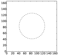
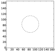
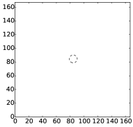
Fig. 1: Circle-case: zero-level set (numerically -0.07-level) of $u^{\epsilon}$ with initial function $u_{0}$ for $T=0$, $T=0.24$ and $T=0.48$.

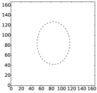
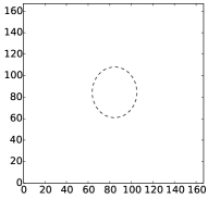
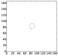
Fig. 2: Ellipse-case: zero-level set (numerically -0.07-level) of $u^{\epsilon}$ with initial function $\tilde{u}_{0}$ for $T=0$, $T=0.24$ and $T=0.36$.

5.5 Discussion of the numerical results

We recall that there are four numerical parameters, i.e. $h$, $\epsilon$, $r_{0}$ and $l_{0}$, in our approach. Incorporating the two space dimensions we are confronted with a de facto five dimensional problem which we discretize. Still, our best error is 0.0139 and in Table 5, attained for the moderate parameter values $h=0.01$, $\Delta t=\epsilon^{2}=0.0004$, $r_{0}=100$ and $l_{0}=360$. We observed that the convergence properties improve when $\gamma$ is closer to $1$.

To classify our errors we compare with [11] where for the Kohn-Serfaty scheme of the curve shortening flow a $l_{\infty}$-error of $0.0078$ is obtained where $\Delta t=0.02$ and $\Delta x=0.0098$ , cf. [11, Table 2]. For the same flow the semi-Lagrangian scheme leads to a $l_{\infty}$-error of $0.00832$, cf. [11, Table 2]. Note, that therein the initial function is a higher order power of the difference $|x|^{2}-R_{0}^{2}$ than in our paper and this effects the error. Furthermore, we refer to [12, Table 1] where a semi-Lagrangian approximation for our equation (2) in the case $\gamma=\frac{1}{3}$ is considered. For $\Delta x=0.01$ and $\Delta t=0.001$ the authors obtain there a $l_{\infty}$-error of $0.0542$ and of $0.0306$ for a modified scheme. Note, that the time interval for the calculation in each of the above cases is—as in our case—approximately $20\%$ of the time interval $[0,T^{*})$ where $T^{*}$ is the time at which the evolving curve ’becomes a point’. Hence our Tables 5 and 6 contain values of adequate size.

References

• [1] L. Alvarez, F. Guichard, P.-L. Lions and J.-M. Morel: Axioms and fundamental equations of image processing. Arch. Rational Mech. Anal., 123, no. 3, 199-257, 1993.
• [2] L. Alvarez and J.-M. Morel: Formalization and computational aspects of image analysis. Acta Numer., Cambridge University Press, Cambridge, UK, pp. 200-257, 1993.
• [3] B. Andrews: Evolving convex curves. Calc. Var. Partial Differential Equations, 7: 315-371, 1998.
• [4] B. Andrews: Classification of limitting shapes for isotropic curve flows. J. Amer. Math. Soc., 16: 443–459, 2003.
• [5] B. Andrews: Contraction of convex hypersurfaces by their affine normal. J. Differ. Geom., 43: 207-230, 1996.
• [6] S. B. Angement, G. Sapiro and A. Tannenbaum: On affine heat equation for non-convex curves. J. Amer. Math. Soc., 11: 601-634, 1998.
• [7] J. W. Barrett, H. Garcke and R. Nürnberg: On the Variational Approximation of Combined Second and Fourth Order Geometric Evolution Equations. SIAM J. Sci. Comput., 29 (3): 1006-1041, 2007.
• [8] J. W. Barrett, H. Garcke and R. Nürnberg: On the parametric finite element approximation of evolving hypersurfaces in $\mathbb{R}^{3}$. J. Comp. Phys., 227 (9): 4281-4307, 2008.
• [9] J. W. Barrett, H. Garcke and R. Nürnberg: Parametric approximation of isotropic and anisotropic elastic flow for closed and open curves. Numer. Math., 120: 489-542, 2012.
• [10] E. Carlini and R. Ferretti: A Semi-Lagrangian Approximation of Min-Max Type for the Stationary Mean Curvature Equation. K. Kunisch, G. Of and O. Steinbach (Eds.): Numerical Methods and Advanced Applications, Springer, pp 679-686, 2008.
• [11] E. Carlini, M. Falcone and R. Ferretti: Convergence of a large time-step scheme for mean curvature motion. Interfaces Free Bound., 12: 409-441, 2010.
• [12] E. Carlini and R. Ferretti: A semi-Lagrangian approximation for the AMSS model of image processing. Appl. Numer. Math., 73: 16-32, 2013.
• [13] Y. G. Chen, Y. Giga and S. Goto: Uniqueness and existence of viscosity solutions of generalized mean curvature flow equations. Proc. Japan. Acad., 65: 207-210, 1989.
• [14] Y. G. Chen, Y. Giga and S. Goto: Uniqueness and existence of viscosity solutions of generalized mean curvature flow equations. J. Differ. Geom., 33, no. 3: 749-786, 1991.
• [15] K.-S. Chou and X.-P. Zhu: The Curve Shortening Problem. Chapman and Hall/CRC, 2000.
• [16] M. G. Crandall, H. Ishii. and P.-L. Lions: User’s guide to viscosity solutions of second order partial differential equations. Bulletin (new Series) of the American Mathematical Society, 27, no. 1: 1-67, 1992.
• [17] K. Deckelnick: Error bounds for a difference scheme approximating viscosity solutions of mean curvature flow. Interfaces Free Bound., 2: 117-142, 2000.
• [18] K. Deckelnick and G. Dziuk: Convergence of a finite element method for non–parametric mean curvature flow. Numer. Math., 72: 197-222, 1995.
• [19] K. Deckelnick, G. Dziuk and C. M. Elliott: Computation of geometric partial differential equations and mean curvature flow. Acta Numer., 14: 139-232, 2005.
• [20] K. Deckelnick and G. Dziuk: Convergence of numerical schemes for the approximation of level set solutions to mean curvature flow. M. Falcone and C. Makridakis (Eds.): Numerical Methods for Viscosity Solutions and Applications, Vol. 59, Series Adv. Math. Appl. Sciences, Springer, pp 77-94, 2001.
• [21] L. C. Evans and J. Spruck: Motion of level sets by mean curvature. J. Differ. Geom., 33: 635–681, 1991.
• [22] Y. Giga: Surface evolution equations. A level set approach. Monographs in Mathematics 99, Birkhäuser Verlag, Basel, 2006.
• [23] Y. Giga and S. Goto: Motion of hypersurfaces and geometric equations. J. Math. Soc. Japan, 44: 99-111, 1992.
• [24] R. Kohn and S. Serfaty: A deterministic-control-based approach to motion by curvature. Commun. Pure Appl. Math., 59, no. 3: 344-407, 2006.
• [25] R. Kohn and S. Serfaty: A deterministic-control-based approach to fully nonlinear parabolic and elliptic equations. Commun. Pure Appl. Math., 63, no. 10: 1298–1350, 2010.
• [26] H. Kröner: Finite element approximation of power mean curvature flow. Preprint, arXiv:1308.2392 [math.NA], 2013.
• [27] A. Kröner, E. Kröner, H. Kröner: Numerical approximation of level set power mean curvature flow. Preprint, arXiv:1503.07382 [math.NA], 2015.
• [28] R. Malladi, J. A: Sethian: Level set methods for curvature flow, image enhancement, and shape recovery in medical images. H. C. Helde, K. Polthier (Eds.): Visualization and Mathematics. Experiments, Simulation and Environments, 329-345, Springer, Berlin, 1997.
• [29] R. Malladi, J. A: Sethian: Image processing: Flows under min/max curvature and mean curvature. Graphical Models and Image Processing, 58: 127–141, 1996.
• [30] K. Mikula, D. Ševčovč: Evolution of plane curves driven by a nonlinear function of curvature and anistropy. SIAM Journal on Applied Mathematics, 61, no. 5: 1473-1501, 2001.
• [31] H. Mitake: On convergence rates for solutions of approximate mean curvature equations. Proceedings of the American Mathematical Society, 139, no. 10: 3691–3696, 2011.
• [32] R. H. Nochetto and C. Verdi: Convergence Past Singularities for a Fully Discrete Approximation of Curvature-Driven Interfaces. SIAM J. Numer. Anal., 34, no. 2: 490-512, 1997.
• [33] K. Osher, J. A. Sethian: Fronts Propagating with Curvature Dependent speed: Algorithms Based on Hamilton-Jacobi Formulation. Journal of Computational Physics, 79: 12-49, 1988.
• [34] G. Sapiro and A. Tannenbaum: On affine plane curve evolution. J. Func. Anal., 119: 79-120, 1994.
• [35] F. Schulze: Evolution of convex hypersurfaces by powers of the mean curvature. Math. Z., 251, no. 4: 721-733, 2005.
• [36] F. Schulze: Nonlinear evolution by mean curvature and isoperimetric inequalities. J. Diff. Geom., 79: 197–241, 2008.
• [37] F. Schulze, appendix with Oliver Schnürer: Convexity estimates for flows by powers of the mean curvature. Ann. Sc. Norm. Super. Pisa Cl. Sci., 5 (5), no 2: 261–277, 2006.
• [38] J. A. Sethian: Theory, Algorithms, and Applications of Level Set Methods for Propagating Interfaces. Acta Numerica, 5: 309-395, 1996.
• [39] J. A. Sethian: Level Set Methods and Fast Marching Methods. Cambridge Monographs on Applied and Computational Mathematics, Vol. 3, Cambridge University Press, 1999.
• [40] N. J. Walkington: Algorithms for computing motion by mean curvature. SIAM J. Numer. Anal, 33: 2215-2238, 1996.