Wireless Compressive Sensing Over Fading Channels with Distributed Sparse Random Projections

Abstract

We address the problem of recovering a sparse signal observed by a resource constrained wireless sensor network under channel fading. Sparse random matrices are exploited to reduce the communication cost in forwarding information to a fusion center. The presence of channel fading leads to inhomogeneity and non Gaussian statistics in the effective measurement matrix that relates the measurements collected at the fusion center and the sparse signal being observed. We analyze the impact of channel fading on nonuniform recovery of a given sparse signal by leveraging the properties of heavy-tailed random matrices. We quantify the additional number of measurements required to ensure reliable signal recovery in the presence of nonidentical fading channels compared to that is required with identical Gaussian channels. Our analysis provides insights into how to control the probability of sensor transmissions at each node based on the channel fading statistics in order to minimize the number of measurements collected at the fusion center for reliable sparse signal recovery. We further discuss recovery guarantees of a given sparse signal with any random projection matrix where the elements are sub-exponential with a given sub-exponential norm. Numerical results are provided to corroborate the theoretical findings.

EDICS: ADEL-DIP, CNS-SPDCN

I Introduction

Consider a wireless sensor network (WSN) deployed to observe a compressible signal. The goal is to reconstruct the observed signal at a distant fusion center utilizing available network resources efficiently. In order to reduce the energy consumption while forwarding observations to a fusion center, some preprocessing is desired so that the fusion center has access to only informative data just querying only a subset of sensors. Use of compressive sensing (CS) techniques for compressible data processing in wireless sensor networks has attracted attention in the recent literature [1, 2, 3, 4, 5, 6, 7, 8, 9, 10, 11, 12, 13]. In [1], the authors have proposed a multiple access channel (MAC) communication architecture so that the fusion center receives a compressed version (represented by a low dimensional linear transformation) of the original signal observed at multiple nodes. According to that model, the corresponding linear operator is a dense random matrix. Thus, almost all the sensors in the network have to participate in forwarding observations consuming a large amount of energy. The application of sparse random matrices to reduce the communication burden for wireless compressive sensing (WCS) has been addressed by several authors [2, 3, 4] so that not all the sensors forward observations. In [11], the authors provide a probabilistic sensor management scheme for target tracking in a WSN exploiting sparse random matrices. In these approaches, the sparse random matrix is considered to be a sparse Rademacher matrix in which elements may take values $(+1,0,-1)$ with desired probabilities. The use of sparse random matrices instead of dense matrices in signal recovery in a general framework (not necessarily in sensor networks) has been further discussed in several works [14, 15, 16, 17].

In practical communication networks, the communication channels between sensor nodes and the fusion center undergo fading. The presence of fading affects the recovery capabilities since it leads to inhomogeneity and non Gaussian statistics in measurement matrices. In [4], the problem of sparse signal recovery in the presence of fading is addressed where the authors provide uniform recovery guarantees based on restricted isometry property (RIP) considering sparse Bernoulli matrices. Two kinds of recovery guarantees with low dimensional random projection matrices are widely discussed in the CS literature [18, 19, 20, 21, 22]: uniform and nonuniform recovery guarantees. A uniform recovery guarantee ensures that for a given draw of the random projection matrix, all possible $k$-sparse signals are recovered with high probability. On the other hand, nonuniform recovery guarantee provides the conditions under which a given $k$-sparse signal (but not any $k$-sparse signal as considered in uniform recovery) can be reconstructed with a given draw of a random measurement matrix. Thus, uniform recovery focuses on the worst case recovery guarantees while nonuniform recovery captures the typical recovery behavior of the measurement matrix.

In this paper, the goal is to enhance our understanding of recovering a given sparse signal with sparse random matrices in the presence of channel fading. More specifically, we provide lower bounds on the number of measurements that should be collected by the fusion center in order to achieve nonuniform recovery guarantees with $l_{1}$ norm minimization based recovery with independent (not necessarily identical) channel fading. With sparse random projections, the nodes transmit their observations with a certain probability. We further discuss how to design probabilities of transmissions by each node (equivalently the sparsity parameter of the random projection matrix) based on the channel fading statistics so that the number of measurements required for signal recovery at the fusion center is minimized.

While the authors in [4] consider a similar problem of WCS, our analysis is different from that in [4] in several ways. In this paper, we derive nonuniform recovery guarantees which require different derivations (not based on RIP) and provide better recovery results compared to uniform recovery as considered in [4]. It is noted that, the RIP measure is defined with respect to the worst-possible performance. Eventhough RIP analysis adopts a probabilistic point of view, the subsequent results tend to be overly restrictive, leading to a wide gap between theoretical predictions and actual performance [20]. With a given signal of interest, one can obtain stronger results. To that end, nonuniform recovery guarantees, as considered in this paper are able to capture the typical recovery behavior of the projection matrix leading to stronger results. We assume envelope detection at the fusion center which is employed in practice in many sensor networks. More specifically, we assume that the channel phase is corrected to ensure phase coherence which is a widely used assumption in the sensor network literature. As discussed in [23, 24], this can be achieved by transmitting a pilot signal by the fusion center before the sensor transmissions to estimate the channel phase. Further, the nonzero elements of the sparse matrices are assumed to be Gaussian. Thus, the statistics of the low dimensional linear operator that relates the input and the output at the fusion center are different from that in [4]. In particular, with the model considered in this paper, the elements of the random projection matrix after taking channel fading into account reduce to independent but nonidentical sub-exponential random variables. To the best of our knowledge, nonuniform recovery of a given sparse signal with nonidentical sub-exponential (or heavy-tailed) random matrices has not been well investigated in the literature. Thus, the analysis in this paper further enhances our understanding on sparse recovery with sub-exponential random matrices in general. Further, we show that the number of measurements required to reconstruct a given sparse signal can be reduced by designing probabilities of transmission at each node based on fading channel statistics. In addition, our results are in general not asymptotic while the results in [4] are asymptotic in nature.

Our main results are summarized below. In the presence of independent channel fading with Rayleigh distribution, we show that the nodes should transmit with a probability that is inversely proportional to the fading channel statistics (channel power) in order to reduce the number of measurements collected at the fusion center in recovering a given sparse signal. With this design of probabilities of transmissions, the number of measurements required to recover a given sparse signal with sparsity index $k$ scales as $\left(\sqrt{\frac{\nu_{\max}^{2}}{\nu_{\min}^{2}}}k\log N\right)$ where $2\nu_{\max}^{2}$ and $2\nu_{\min}^{2}$ are the largest and smallest average mean power coefficients of Rayleigh fading channels, and $N$ is the number of nodes in the network (which is assumed to be the same as the dimension of the sparse signal). This says, by controlling the probability of transmission based on fading channel statistics, the impact of inhomogeneity of the elements of the measurement matrix on signal recovery can be reduced leading to better recovery guarantees. In the special case where the fading channels are assumed to be identical and all the nodes transmit with the same probability (say $0<\gamma\leq 1$), we show that $\mathcal{O}\left(\frac{k}{\sqrt{\gamma}}\log N\right)$ MAC transmissions are sufficient to recover a given sparse signal. We further, provide detailed analysis on recovery guarantees of a given sparse signal with any random projection matrix where the elements are sub-exponential with a given sub-exponential norm.

The rest of the paper is organized as follows. In Section II, the problem formulation is given. Recovery guarantees of a given sparse signal under independent channel fading are provided in Section III. We discuss how to design probabilities of transmission based on channel fading statistics. Further, the results are specified when the fading channels are identical. In Section IV, the conditions under which a given sparse signal can be recovered with any sub-exponential random matrix are discussed. Numerical results are presented in Section V and concluding remarks are given in Section VI.

I-A Notation

The following notation is used throughout the paper. Lower case boldface letters, e.g., $\mathbf{x}$ are used to denote vectors and the $j$-th element of $\mathbf{x}$ is denoted by $\mathbf{x}(j)$. Lower case letters are used to denote scalars, e.g., $x$. Both upper case boldface letters and boldface symbols are used to denote matrices, e.g., $\mathbf{A}$, $\bm{\Phi}$. The notations, $\mathbf{A}_{i}$, $\mathbf{a}_{i}$ and $\mathbf{A}_{ij}$ are used to denote the $i$-th row, $i$-th column and the $(i,j)$-th element of the matrix $\mathbf{A}$, respectively. The transpose of a matrix or a vector is denoted by $(.)^{T}$ and $(\mathbf{A})^{\dagger}$ denotes the Moore-Penrose pseudo inverse of $\mathbf{A}$. The notation $\otimes$ denotes the outer product of two vectors. Upper case letters with calligraphic font, e.g., $\mathcal{S}$, are used to denote sets. The $l_{p}$ norm of a vector $\mathbf{x}$ is denoted by $||\mathbf{x}||_{p}$. The spectral norm of a matrix $\mathbf{A}$ is denoted by $||\mathbf{A}||$. We use the notation $|.|$ to denote the absolute value of a scalar, as well as the cardinality of a set. We use $\mathbf{I}_{N}$ to denote the identity matrix of dimension $N$ (we avoid using subscript when there is no ambiguity). A diagonal matrix in which the main diagonal consists of the vector $\mathbf{x}$ is denoted by $\mathrm{diag}(\mathbf{x})$. By $s_{\min}(\mathbf{A})$ and $s_{\max}(\mathbf{A})$, we denote the minimum and maximum singular values, respectively, of the matrix $\mathbf{A}$. The notation $\mathrm{Rayleigh}(\sigma)$ denotes that a random variable $x$ has a Rayleigh distribution with the probability density function (pdf) $f(x)=\frac{x}{\sigma^{2}}e^{-\frac{x^{2}}{2\sigma^{2}}}$ for $x\geq 0$. The notation $x\sim\mathcal{N}(\mu,\sigma^{2})$ denotes that the random variable $x$ is distributed as Gaussian with the pdf $f(x)=\frac{1}{\sqrt{2\pi\sigma^{2}}}e^{-\frac{(x-\mu)^{2}}{2\sigma^{2}}}$.

II Problem Formulation

II-A Observation model

Consider a distributed sensor network measuring compressible (sparse) data using $N$ number of nodes. The observation collected at the $i$-th sensor node is denoted by $x_{i}$ for $i=0,1,\cdots,N-1$. Let $\mathbf{x}=[x_{0},\cdots,x_{N-1}]^{T}$ be the vector containing all the measurements of sensors. Sparsity is a common characteristic observed with the data collected in sensor networks. The sparsity may appear as an inherent property of the signal being observed by multiple sensors, e.g., most acoustic data has a sparse representation in Fourier domain. On the other hand, not all the observations collected at nodes are informative; for example, the sensors located far away from the phenomenon being observed may contain poor observations making the observation vector $\mathbf{x}$ sparse in the canonical basis. In a general framework, assume that the signal $\mathbf{x}$ is sparse in some basis $\bm{\Phi}$. One of the fundamental tasks in many sensor networking applications is to reconstruct the signal observed by nodes at a distant fusion center. Due to inherent resource constraints in sensor networks, it is desirable that sensors use only small amount of energy and low bandwidth while forwarding information to the fusion center. With recent advances in the theory of CS, WCS with random measurement matrices is becoming attractive. A compressed version of $\mathbf{x}$ can be transmitted to a fusion sensor exploiting coherent transmission schemes developed for sensor networks [1].

Consider that the $j$-th sensor multiplies its observation during the $i$-th transmission by $\mathbf{A}_{ij}$ which is a scalar (to be defined later). All the nodes transmit their scaled observations coherently using $M$ (time or frequency) slots. In this paper, we consider the amplify-and-forward (AF) approach for sensor transmissions. It is noted that a digital approach can be used where we digitize the observation into bits, possibly apply channel coding, and then use digital modulation schemes to transmit the data, for example, as considered in [25]. However, as shown in [26] for a single Gaussian source with an AWGN channel, the AF approach is optimal. Analog transmission schemes over MAC for detection and estimation using WSN have been widely investigated, for example, in [27, 28, 29]. Thus, we restrict our analysis in this paper to analog transmission, while digital modulated signals will be considered in a future work. We further assume that the channels between the sensors and the fusion center undergo flat fading. We further assume phase coherent reception, thus the effect of fading is reflected as a scalar multiplication. The received signal at the fusion center with the $i$-th MAC transmission is given by,

$$y_{i}=\sum_{j=0}^{N-1}h_{ij}\mathbf{A}_{ij}x_{j}+v_{i}$$ (1)

for $i=0,1,\cdots,M-1$ where $h_{ij}$ is the channel coefficient for the channel between the $j$-th sensor and the fusion center during the $i$-th transmission and $v_{i}$ is the additive noise with mean zero and variance $\sigma_{v}^{2}$.

Due to energy constraints in sensor networks, we consider a scenario where not all the nodes transmit during each MAC transmission. To achieve this, $\mathbf{A}_{ij}$ is selected as:

$$\mathbf{A}_{ij}=\left\{\begin{array}[]{cc}a_{ij}&\mathrm{with}~{}\mathrm{prob}~{}\gamma_{j}\\ 0&\mathrm{with}~{}\mathrm{prob}~{}1-\gamma_{j}\end{array}\right.$$ (4)

where $a_{ij}\sim\mathcal{N}(0,\sigma_{j}^{2})$ and $0<\gamma_{j}\leq 1$ is the probability of transmission of the $j$-th node. The average power used by the $j$-th sensor during the $i$-th MAC transmission is $\mathbb{E}\{\mathbf{A}_{ij}^{2}\}=\gamma_{j}\sigma_{j}^{2}$ which is assumed to be less than $E_{j}$ where $E_{j}$ is determined based on the available energy at the $j$-th node. We assume that the $j$-th node uses the same transmit power on an average during all MAC transmissions. Let $\mathbf{A}$ be a $M\times N$ matrix in which $(i,j)$-th element is given by $\mathbf{A}_{ij}$ as in (4). Further, let $\mathbf{H}$ be a $M\times N$ matrix in which $(i,j)$-th element is given by $h_{ij}$. With vector-matrix notation, (1) can be written as,

$$\mathbf{y}=\mathbf{B}\mathbf{x}+\mathbf{v}$$ (5)

where $\mathbf{B}=\mathbf{H}\odot\mathbf{A}$, $\odot$ is the Hadamard (element-wise) product, $\mathbf{y}=[y_{0},\cdots,y_{M-1}]^{T}$ and $\mathbf{v}=[v_{0},\cdots,v_{M-1}]^{T}$. Let $\bm{\gamma}=[\gamma_{0},\cdots,\gamma_{N-1}]^{T}$. The vector $\bm{\gamma}$ is used to refer to the measurement sparsity of the matrix $\mathbf{B}$ or equivalently the probabilities of transmission of all the nodes. The goal is to recover $\mathbf{x}$ based on (5). One of the widely used approaches for sparse recovery is to solve the following optimization problem [21]:

$$\underset{\mathbf{x}}{\min}||\mathbf{x}||_{1}~{}\mathrm{such}~{}\mathrm{that}~{}\mathbf{y}=\mathbf{B}\mathbf{x}$$ (6)

with no noise, or

$$\underset{\mathbf{x}}{\min}||\mathbf{x}||_{1}~{}\mathrm{such}~{}\mathrm{that}~{}||\mathbf{y}-\mathbf{B}\mathbf{x}||_{2}\leq\epsilon_{v}$$ (7)

with noise where $\epsilon_{v}$ bounds the size of the noise term $\mathbf{v}$.

It is noted that, when $\gamma_{j}=1$ and $\sigma_{j}^{2}=\sigma_{a}^{2}$ for all $j$, the elements of $\mathbf{A}$ are independent and identically distributed (iid) Gaussian with mean zero and variance $\sigma_{a}^{2}$. Then, if we further assume AWGN channels so that $\mathbf{B}=\mathbf{A}$, $\mathbf{B}$ is a random matrix with iid Gaussian random variables. Sparse signal recovery with iid Gaussian random matrices has been extensively studied [21, 20]. Under fading, the matrix $\mathbf{A}$ is multiplied (element-wise) by another random matrix $\mathbf{H}$ which has independent and nonidentical elements. Thus, the recovery capability of (6) (or (7)) depends on the properties of the matrix $\mathbf{B}=\mathbf{H}\odot\mathbf{A}$. In this paper, we assume that the fading coefficients $h_{ij}$ are independent Rayleigh random variables with $h_{ij}\sim\mathrm{Rayleigh}(\nu_{j})$ for $i=0,\cdots,M-1$ and $j=0,1,\cdots,N-1$ where $\mathbb{E}\{h_{ij}^{2}\}=2\nu_{j}^{2}$ is assumed to be different in general for the channels between different sensors and the fusion center. The goal is to obtain recovery guarantees of a given $\mathbf{x}$ based on (6) under the above discussed statistics for $\mathbf{A}$ and $\mathbf{H}$.

First, it is important to observe the statistical properties of the matrix $\mathbf{B}$.

II-B Statistics of $\mathbf{B}$

The $(i,j)$-th element of $\mathbf{B}$ is given by,

$$\mathbf{B}_{ij}=\left\{\begin{array}[]{cc}h_{ij}a_{ij}&\mathrm{with}~{}\mathrm{prob}~{}\gamma_{j}\\ 0&\mathrm{with}~{}\mathrm{prob}~{}1-\gamma_{j}\end{array}\right.$$ (10)

for $i=0,\cdots,M-1$ and $j=0,\cdots,N-1$. Since the elements of $\mathbf{A}$ and $\mathbf{H}$ are assumed to be independent, the elements of $\mathbf{B}$ are also independent (but not identical in general).

Proposition 1.

Let $w=h_{ij}a_{ij}$ where $a_{ij}\sim\mathcal{N}(0,\sigma_{a}^{2})$ and $h_{ij}\sim\mathrm{Rayleigh}(\nu_{h})$. Then the pdf of $w$ is doubly exponential (Laplacian) which is given by,

$$f(w)=\frac{1}{2\bar{\sigma}}e^{-{\frac{1}{\bar{\sigma}}}|w|}.$$

where $\bar{\sigma}=\nu_{h}\sigma_{a}$.

Proof.

See Appendix A. ∎

Taking $\bar{\sigma}_{j}=\sigma_{j}\nu_{j}$, the pdf of $u=\mathbf{B}_{ij}$ in (10) can be written as

$$f(u)=\gamma_{j}\frac{1}{2\bar{\sigma}_{j}}e^{-\frac{|u|}{\bar{\sigma}_{j}}}+(1-\gamma_{j})\delta(u)$$ (11)

where $\delta(.)$ is the Dirac delta function. It can be easily proved that

$$Pr(|u|>t)=\left\{\begin{array}[]{ccc}1{}&for~{}t=0\\ \gamma_{j}e^{-\frac{t}{\bar{\sigma}_{j}}}{}&for~{}t>0\end{array}\right..$$

Thus, we can find a constant $K_{1}>0$ such that,

$$Pr(|u|>t)\leq e^{1-t/K_{1}}$$

for all $t\geq 0$. Thus, $u$ is a sub-exponential random variable [30]. In other words, the elements of $\mathbf{B}$ are independent (but not identical in general) sub-exponential random variables. While there is a substantial amount of work in the literature that addresses the problem of sparse signal recovery with Gaussian and sub-Gaussian random matrices, very little is known with random matrices with sub-exponential (or heavy tailed) elements. In the following, we obtain nonuniform recovery guarantees for (6) when the elements of $\mathbf{B}$ have a pdf as given in (11) and simplify the results when the matrix $\mathbf{B}$ is isotropic. We further provide recovery guarantees for general nonidentical sub-exponential random matrices.

III Nonuniform Recovery Guarantees with Independent Channel Fading

We present the following statistical results which are helpful in deriving recovery conditions.

Definition 1 (Isotropic random vectors [20]).

A random vector $\mathbf{x}\in\mathbb{R}^{N}$ is called isotropic if $\mathbb{E}\{\mathbf{x}\mathbf{x}^{T}\}=\mathbf{I}_{N}$.

The row vectors of the matrix $\mathbf{B}$ are in general not isotropic. However, the column vectors of $\mathbf{B}$ with appropriate normalization become isotropic. In the special case where $\gamma_{j}=\gamma$ and $\bar{\sigma}_{j}=\bar{\sigma}$, both row and columns vectors of the normalized matrix $\frac{1}{\sqrt{2\gamma\bar{\sigma}^{2}}}\mathbf{B}$ are isotropic.

Proposition 2 (mgf $u$).

Let $u$ be a random variable with pdf $f(u)$ where $f(u)$ is given in (11). Then for $|t|\leq\frac{1}{\tilde{\eta}_{\max}}$ where $\tilde{\eta}_{\max}=\underset{j}{\max}\{\bar{\sigma}_{j}\}$, we have

$$\mathbb{E}\{e^{tu}\}\leq e^{\eta_{\max}t^{2}}$$

where $\eta_{\max}=\underset{j}{\max}\{\gamma_{j}\bar{\sigma}_{j}^{2}\}$.

Proof.

See Appendix B. ∎

Next, we provide a Bernstein-type inequality to bound the weighted sum of independent but nonidentical random variables with pdf as given in (11). It is noted that, a similar bound is derived in [30] for general sub-exponential random variables which are characterized by the sub-exponential norm. The following results are the same as those in Proposition $5.16$ of [30] only when $\gamma_{j}=1$ for all $j$.

Proposition 3 (Bernstein-type inequality ).

Let $u_{0},\cdots,u_{N-1}$ be $N$ independent random variables where the pdf of $u_{j}$ is as given in (11) for $j=0,\cdots,N-1$. Then for every $\bm{\alpha}=(\alpha_{0},\cdots,\alpha_{N-1})\in\mathbb{R}^{N}$ and every $t>0$, we have,

$$Pr\left(|\sum_{i=0}^{N-1}\alpha_{i}u_{i}|\geq t\right)\leq 2e^{-\min\left(\frac{t^{2}}{4\eta_{\max}||\bm{\alpha}||_{2}^{2}},\frac{t}{2\tilde{\eta}_{\max}||\bm{\alpha}||_{\infty}}\right)}$$ (13)

where $\eta_{\max}=\underset{j}{\max}\{\gamma_{j}\bar{\sigma}_{j}^{2}\}$ and $\tilde{\eta}_{\max}=\underset{j}{\max}\{\bar{\sigma}_{j}\}$ as defined before.

Proof.

See Appendix C. ∎

III-A Nonuniform recovery guarantees in the presence of independent fading channels

In the following, we present our main results on recovery of a given $\mathbf{x}$ based on (6). Before that, we introduce additional notation. Let $\mathcal{U}=\{0,1,\cdots,N-1\}$ and $\mathcal{S}:=\mathrm{supp}(\mathbf{x})=\{i:\mathbf{x}(i)\neq 0,i=0,1,\cdots,N-1\}$ where $\mathbf{x}(i)$ is the $i$-th element of $\mathbf{x}$. For a $k$-sparse vector $\mathbf{x}$, we have $|\mathcal{S}|=k$. Further, by $\mathbf{B}_{S}$, we denote the sub-matrix of $\mathbf{B}$ that contains columns of $\mathbf{B}$ corresponding to the indices in $\mathcal{S}$ and $\mathbf{x}^{S}$ is a $k\times 1$ vector which contains the elements of $\mathbf{x}$ corresponding to indices in $\mathcal{S}$. Further, let $\bar{\bm{\sigma}}=[\bar{\sigma}_{0},\cdots,\bar{\sigma}_{N-1}]^{T}$ and $\bm{\nu}=[\nu_{0},\cdots,\nu_{N-1}]^{T}$.

To ensure recovery of a given signal $\mathbf{x}$ via (6), it is sufficient to show that [31, 32, 22],

$$|\langle(\mathbf{B}_{S})^{\dagger}\mathbf{b}_{l},\mathrm{sgn}(\mathbf{x}^{S})\rangle|<1~{}\mathrm{for}~{}\mathrm{all}~{}l\in\mathcal{U}\setminus\mathcal{S}$$

where $(\mathbf{B}_{S})^{\dagger}=(\mathbf{B}_{S}^{T}\mathbf{B}_{S})^{-1}\mathbf{B}_{S}^{T}$ is the Moore-Penrose pseudo inverse of $\mathbf{B}_{S}$ and $\mathrm{sgn}(\mathbf{x})$ is the sign vector having entries

$$\mathrm{sgn}(\mathbf{x})_{j}:=\left\{\begin{array}[]{ccc}\frac{\mathbf{x}_{j}}{|\mathbf{x}_{j}|}{}&\mathrm{if}~{}\mathbf{x}(j)\neq 0,\\ 0,{}&\mathrm{otherwise},\end{array}\right.\mathrm{for}~{}\mathrm{all}~{}j\in\mathcal{U}.$$

Theorem 1.

Let $\mathcal{S}\subset\mathcal{U}$ with $|\mathcal{S}|=k$. Further, let the elements of $\mathbf{B}$ be given as in (10), $\eta_{\max}(\bm{\gamma},\bar{\bm{\sigma}})=\underset{0\leq j\leq N-1}{\max}(\gamma_{j}\bar{\sigma}_{j}^{2})$, $\eta_{\min}(\bm{\gamma},\bar{\bm{\sigma}})=\underset{0\leq j\leq N-1}{\min}(\gamma_{j}\bar{\sigma}_{j}^{2})$ and $\tilde{\eta}_{\max}(\bar{\bm{\sigma}})=\underset{0\leq j\leq N-1}{\max}\{\bar{\sigma}_{j}\}$. Define $R$ such that

$$\frac{||\mathbf{b}_{S}||_{\infty}}{||\mathbf{b}_{S}||_{2}}\leq R$$

almost surely where $0<R\leq 1$ and $\mathbf{b}_{S}=(\mathbf{B}_{\mathcal{S}}^{\dagger})^{T}\mathrm{sgn}(\mathbf{x}^{S})$. Then, for $0<\epsilon,\epsilon^{\prime}<1$, $\mathbf{x}$ is the unique solution to (6) with probability exceeding $1-\max(\epsilon,\epsilon^{\prime})$ if the following condition is satisfied:

$$M\geq\max\{M_{1},M_{2}\}$$ (15)

where $M_{1}$ and $M_{2}$ are given in (16) and (17) respectively,

$$M_{1} = \frac{\eta_{\max}(\bm{\gamma},\bar{\bm{\sigma}})}{\eta_{\min}(\bm{\gamma},\bar{\bm{\sigma}})}2k\left(\sqrt{\frac{\eta_{\max}(\bm{\gamma},\bar{\bm{\sigma}})}{\eta_{\min}(\bm{\gamma},\bar{\bm{\sigma}})}}\sqrt{\log(2N/\epsilon)}+\sqrt{\frac{\log(k/\epsilon^{\prime})}{2c^{\prime}}}\right)^{2}$$ (16)

$$M_{2} = \frac{\eta_{\max}(\bm{\gamma},\bar{\bm{\sigma}})}{\eta_{\min}(\bm{\gamma},\bar{\bm{\sigma}})}2k\left(\frac{\tilde{\eta}_{\max}(\bar{\bm{\sigma}})}{\sqrt{\eta_{\min}(\bm{\gamma},\bar{\bm{\sigma}})}}R{\log(2N/\epsilon)}+\sqrt{\frac{\log(k/\epsilon^{\prime})}{2c^{\prime}}}\right)^{2}$$ (17)

and $c^{\prime}$ is an absolute constant.

Proof.

See Appendix D. ∎

From Theorem 1, it is observed that the ratio between peak and total energy of $\mathbf{b}_{S}$, $R$, plays an important role in deciding the minimum number of MAC transmissions needed to recover $\mathbf{x}$ with a given support $\mathcal{S}$. As shown in Appendix E, when the elements of $\mathbf{B}$ are distributed according to (11) we can take

$$R=\mathcal{O}\left(\sqrt{\frac{k}{2M}}\right).$$

Then, the dominant part of $M_{2}$ in (17) scales as

$$\mathcal{O}\left(\sqrt{\frac{\eta_{\max}(\bm{\gamma},\bar{\bm{\sigma}})\tilde{\eta}^{2}_{\max}(\bar{\bm{\sigma}})}{\eta^{2}_{\min}(\bm{\gamma},\bar{\bm{\sigma}})}}k{\log(2N/\epsilon)}\right)$$ (18)

while the dominant term of $M_{1}$ scales as

$$\mathcal{O}\left(\frac{\eta^{2}_{\max}(\bm{\gamma},\bar{\bm{\sigma}})}{\eta^{2}_{\min}(\bm{\gamma},\bar{\bm{\sigma}})}k{\log(2N/\epsilon)}\right).$$ (19)

Thus, when

$$\underset{j}{\min}\{\gamma_{j}\bar{\sigma}_{j}^{2}\}\leq\underset{j}{\max}\{\gamma_{j}\bar{\sigma}_{j}^{2}\}\frac{\sqrt{\underset{j}{\max}\{\gamma_{j}\bar{\sigma}_{j}^{2}\}}}{\underset{j}{\max}\{\bar{\sigma}_{j}\}}$$ (20)

$M_{1}$ dominates $M_{2}$ (and vice versa).

III-B Probabilities of transmission and channel fading statistics

From (18) and (19), it is seen that the number of MAC transmissions required for reliable signal recovery depends on the probabilities of transmission $\bm{\gamma}$, and the quality of the fading channels $\bm{\nu}$. Since the designer has the control on $\bm{\gamma}$, we discuss how to design $\bm{\gamma}$ as a function of $\bm{\nu}$ so that $M_{1}$ and $M_{2}$ become minimum with respect to $\bm{\gamma}$. Since $\eta_{\max}\geq\eta_{\min}$, for $M_{1}$ and $M_{2}$ to be minimum, it is desired to have the gap between $\eta_{\max}$ and $\eta_{\min}$ minimum. When $\eta_{\max}=\eta_{\min}$, it is easily seen that $M_{2}$ dominates $M_{1}$, thus, $M=M_{2}$. Let us assume that the maximum available energy at each node for given transmission is the same so that $\sigma_{j}^{2}=\sigma_{a}^{2}$ and $E_{j}=E$ for all $j$. Then the probability of transmission at each node should satisfy the following condition:

$$\gamma_{j}\leq\min\left\{1,\frac{E}{\sigma_{a}^{2}}\right\}=\bar{\gamma}$$ (21)

for $j=0,\cdots,N-1$.

When $\sigma_{j}^{2}=\sigma_{a}^{2}$ for all $j$, the term that depends on $\bm{\gamma}$ in $M_{2}$ in (18) can be expressed as,

$$\Psi(\bm{\gamma})=\sqrt{\frac{\eta_{\max}(\bm{\gamma},\bar{\bm{\sigma}})\tilde{\eta}^{2}_{\max}(\bar{\bm{\sigma}})}{\eta^{2}_{\min}(\bm{\gamma},\bar{\bm{\sigma}})}}=\sqrt{\frac{\underset{j}{\max}\{\gamma_{j}\nu_{j}^{2}\}\underset{j}{\max}\{\nu_{j}^{2}\}}{\left(\underset{j}{\min}\{\gamma_{j}\nu_{j}^{2}\}\right)^{2}}}.$$ (22)

Since $\gamma_{j}\leq 1$ for all $j$, we have $\Psi(\bm{\gamma})\geq 1$ and the equality (of $\Psi(\bm{\gamma})\geq 1$ where $\Psi(\bm{\gamma})$ is given in (22)) holds only if $\gamma_{j}=1$ for all $j$ and the channels are identical so that $\nu_{0}^{2}=\nu_{1}^{2}=\cdots,\nu_{N-1}^{2}$. The goal is to find $\bm{\gamma}$ so that (22) is minimized under the constraint (21). It is noted that $\Psi(\bm{\gamma})$ is minimum with respect to $\bm{\gamma}$ when $\underset{j}{\max}\{\gamma_{j}\nu_{j}^{2}\}=\underset{j}{\min}\{\gamma_{j}\nu_{j}^{2}\}$. Without loss of generality, we sort $\nu_{j}$’s in ascending order so that $\nu_{1}\leq\nu_{2}\leq\cdots,\nu_{N}$. To achieve $\underset{j}{\max}\{\gamma_{j}\nu_{j}^{2}\}=\underset{j}{\min}\{\gamma_{j}\nu_{j}^{2}\}$, we select $\bm{\gamma}$ so that the largest $\gamma_{j}$ is assigned to the node indexed by $0$ while the smallest $\gamma_{j}$ is assigned to the node indexed by $N-1$ for $j=0,\cdots,N-1$. More specifically, let $\gamma_{j}=\frac{d_{0}}{\nu_{j}}$ for $j=0,\cdots,N-1$ where $d_{0}$ is a constant. This leads to

$$\Psi(\bm{\gamma})=\sqrt{\frac{\nu_{N-1}^{2}}{d_{0}}}.$$ (23)

With the constraint for $\gamma_{j}$ in (21), we further have

$$d_{0}\leq\bar{\gamma}\nu_{0}^{2}.$$

Then, $\Psi(\bm{\gamma})$ in (23) is minimum when $d_{0}=\bar{\gamma}\nu_{0}^{2}$. Thus, the probabilities of transmission which minimize $\Psi(\bm{\gamma})$ are given by

$$\gamma_{j}^{\mathrm{opt}}=\bar{\gamma}\frac{\nu_{0}^{2}}{\nu_{j}^{2}}$$ (24)

for $j=0,\cdots,N-1$ and the minimum value of $\Psi(\bm{\gamma})$ is

$$\Psi(\bm{\gamma}^{\mathrm{opt}})=\sqrt{\frac{\nu_{N-1}^{2}}{\bar{\gamma}\nu_{0}^{2}}}.$$

With this design of $\bm{\gamma}$, the number of MAC transmissions required for reliable signal recovery at the fusion center scales as

$$M=\mathcal{O}\left(\sqrt{\frac{C_{1}(\bm{\nu})}{\bar{\gamma}}}k{\log(2N/\epsilon)}\right)$$ (25)

where $C_{1}(\bm{\nu})=\frac{\underset{j}{\max}\{\nu_{j}^{2}\}}{\underset{j}{\min}\{\nu_{j}^{2}\}}$ Thus, the impact of inhomogeneous channel fading with the optimal design of $\bm{\gamma}$ on $M$ appears as the ratio between $\underset{j}{\max}\{\nu_{j}\}$ and $\underset{j}{\min}\{\nu_{j}\}$.

III-C Nonuniform recovery when $\mathbf{B}$ is dense

Here we study the special case where $\gamma_{j}=1$ for $j=0,\cdots N-1$ so that $\mathbf{B}$ is a dense matrix. In this case, $M_{1}$ in (19) dominates $M_{2}$ in (18). Thus, $M=M_{1}$ and we have,

$$M=\mathcal{O}\left(C_{2}(\bm{\nu})k{\log(2N/\epsilon)}\right)$$ (26)

where $C_{2}(\bm{\nu})=\left(\frac{\underset{j}{\max}\{\nu_{j}^{2}\}}{\underset{j}{\min}\{\nu_{j}^{2}\}}\right)^{2}$ and we assume $\sigma_{j}^{2}=\sigma_{a}^{2}$ for all $j$. Note that in this case $\bar{\gamma}=1$. From (25) and (26), it is seen that the scaling of $M$ when $\gamma=1$ is greater than that is with a sparse matrix with properly designed probabilities transmission since $C_{2}(\bm{\nu})\geq C_{1}(\bm{\nu})$. This implies that, with nonidentical fading channels, it is beneficial to use sparse random projections with transmission probabilities matched to fading statistics as in (24) compared to the use of dense matrices in order to reduce the total number of MAC transmissions. While (26) provides a scaling, the exact $M$ required for reliable sparse signal recovery is illustrated in numerical results section (Fig. 4) for dense and sparse matrices with nonidentical channels.

As will be shown in the next section, when the matrix $\mathbf{B}$ has dense iid elements (so that $\gamma_{j}=1$ for $j=0,\cdots N-1$ and $\nu_{0}^{2}=\cdots=\nu_{N-1}^{2}$), we get $M=\mathcal{O}(k\log(2N/\epsilon))$. From (25) and (26), it is seen that, the presence of non identical fading channels (the inhomogeneity) increases the required number of MAC transmissions by a factor of $\sqrt{\frac{C_{1}(\bm{\nu})}{\bar{\gamma}}}$ with sparse projections and $C_{2}(\bm{\nu})$ with dense projections, respectively, compared to that required with identical channels. It is further worth mentioning that we obtain dominant parts of $M_{1}$ and $M_{2}$ as in (19) and (18) using lower bounds for (16) and (17), respectively. Thus, the impact of $C_{1}(\bm{\nu})$ and $C_{2}(\bm{\nu})$ on (25) and (26), respectively, can be scaled versions of them.

III-D Nonuniform recovery when $\mathbf{B}$ is isotropic

Now consider the special case where $\gamma_{j}=\gamma$, $\bar{\sigma}_{j}=\bar{\sigma}=\sigma_{a}\nu_{h}$ for all $j$. Then, the elements of $\mathbf{B}$ are iid random variables and the columns and rows of the scaled random matrix $\frac{1}{\sqrt{2\gamma\bar{\sigma}^{2}}}\mathbf{B}$ are isotropic. From Theorem 1, we have the following Corollary.

Corollary 1.

Assume $\gamma_{j}=\gamma$ and $\bar{\sigma}_{j}=\bar{\sigma}$ for all $j$. Then when

$$M=\mathcal{O}\left(\frac{k}{\sqrt{\gamma}}\log(2N/\epsilon)\right)$$ (27)

$\mathbf{x}$ can be uniquely determined based on (6) with high probability, where $0<\epsilon<1$ is as defined in Theorem 1.

Proof.

When $\gamma_{j}=\gamma$ and $\bar{\sigma}_{j}=\bar{\sigma}$ for all $j$, we have $\eta_{\min}=\eta_{\max}=\gamma\bar{\sigma}^{2}$ and $\tilde{\eta}_{\max}=\bar{\sigma}$. Then, the scaling of $M_{1}$ in (19) reduces to $\mathcal{O}\left(k\log(2N/\epsilon)\right)$ while the scaling of $M_{2}$ in (18) reduces to $\mathcal{O}\left(\frac{k}{\sqrt{\gamma}}\log(2N/\epsilon)\right)$0. Since $\gamma\leq 1$, $M_{2}$ dominates $M_{1}$. ∎

When $\gamma=1$, the matrix $\mathbf{B}$ is dense and the elements are iid doubly exponential. Then $\mathcal{O}(k\log(2N/\epsilon))$ measurements are sufficient for reliable recovery of $\mathbf{x}$. As $\gamma$ decreases, equivalently when the matrix $\mathbf{B}$ becomes more sparse, the minimum $M$ required for sparse signal recovery increases. In particular, when $\gamma<1$, the product $\gamma k$ plays an important role in determining $M$. It is noted that $\gamma k$ reflects the average number of nonzero coefficients of $\mathbf{x}$ that align with the nonzero coefficients in each row of the sparse projection matrix $\mathbf{B}$. In Table I, we summarize the scalings of $M$ required for recovery of $\mathbf{x}$ in different regimes of $\gamma k$. In particular,

• when $\gamma k=\tau_{0}$ where $\tau_{0}$ is a constant, we have $\gamma\propto\frac{1}{k}$. Then, when $k$ is sublinear with respect to $N$ so that $k=o(N)$, $\mathcal{O}(k^{3/2}\log(N))$ measurements are sufficient for reliable recovery of given $\mathbf{x}$. It is noted that this scaling is only slightly greater than $\mathcal{O}(k\log(N))$ which is the scaling required for a dense matrix with iid elements. This observation is intuitive since, when $k=o(N)$, $\gamma$ is not very small and the matrix $\mathbf{B}$ is not ’very’ sparse. On the other hand, when $k$ is linear with respect to $N$ so that $k=\Theta(N)$, and $\gamma\propto\frac{1}{k}$, $\mathcal{O}(N^{3/2}\log(N))$ measurements are required.

• when $\gamma k=\varepsilon N$ with $0<\varepsilon<\frac{k}{N}$, it is required to have $\mathcal{O}\left(\frac{k^{3/2}}{\sqrt{\varepsilon N}}\log(N)\right)$ measurements when $k=o(N)$. It is noted that, with this setting we have $\varepsilon<\frac{k}{N}$ and $\varepsilon\rightarrow 0$ as $N\rightarrow\infty$. On the other hand, when $k=\Theta(N)$ and $\gamma k=\varepsilon N$ with $0<\varepsilon<\frac{k}{N}$, $M$ should be scaled as $\mathcal{O}\left(\frac{N}{\sqrt{\varepsilon}}\log(N)\right)$. With this setting $\varepsilon<\Theta(1)$, thus, $\mathcal{O}(N\log(N))$ measurements are needed for reliable recovery of $\mathbf{x}$.

TABLE I: Minimum M in the different regimes of $\gamma k$

$\gamma k$	$M$ when $k=o(N)$	$M$ when $k=\Theta(N)$
$\gamma k=\tau_{0}$	$\mathcal{O}\left(k^{3/2}\log(N)\right)$	$\mathcal{O}(N^{3/2}\log(N))$
$\gamma k=\varepsilon N$	$\mathcal{O}\left(\frac{k^{3/2}}{\sqrt{\varepsilon N}}\log(N)\right)$	$\mathcal{O}\left(\frac{N}{\sqrt{\varepsilon}}\log(N)\right)$
$0<\varepsilon<\frac{k}{N}$

III-D1 Design of $\gamma$ under total network energy constraints

For given $M$, the average energy required by the network to achieve complete sparse signal recovery in the presence of iid fading channels is given by,

$$E_{req}=M\gamma N\sigma_{a}^{2}.$$

For complete signal recovery with probability at least $1-\epsilon$, we should have

$$M\geq C_{0}\frac{k}{\sqrt{\gamma}}\log(2N/\epsilon)$$

where $C_{0}$ is a constant. Then, we have,

$$E_{req}\geq\sqrt{\gamma}C_{0}\sigma_{a}^{2}kN\log(2N/\epsilon).$$ (28)

Assume that the network is subject to a total energy constraint so that we have to make sure,

$$E_{req}\leq\bar{E}.$$

Then, $\gamma$ should satisfy the following constraint:

$$\sqrt{\gamma}\leq\min\left\{1,\frac{\bar{E}}{C_{0}\sigma_{a}^{2}kN\log(2N/\epsilon)}\right\}.$$

IV Nonuniform Recovery Guarantees with General Sub-exponential Matrices

In the following, we consider recovering $\mathbf{x}$ from $\mathbf{y}=\mathbf{B}\mathbf{x}+\mathbf{v}$ when the elements of $\mathbf{B}$ are general sub-exponential random variables and the rows of $\mathbf{B}$ are non-isotropic.

First, let us define the sub-exponential norm of a sub-exponential random variable which will be helpful in the following analysis.

Definition 2 (sub-exponential norm [30]).

Let $x$ be a sub-exponential random variable. The sub-exponential norm of $x$, $||x||_{\psi_{1}}$, is defined by

$$||x||_{\psi_{1}}=\underset{p\geq 1}{\sup}~{}\frac{1}{p}(\mathbb{E}\{|x|^{p}\})^{1/p}.$$

Further, let us assume that the each row of $\mathbf{B}$ has the same second moment matrix $\Sigma_{B}$. Then, we have the following Theorem.

Theorem 2.

Let $\mathbf{x}$ be a $k$-sparse vector with the support set $\mathcal{S}$ and the matrix $\mathbf{B}$ contain independent sub-exponential random variables. Let $\rho_{\max}$ denotes the maximum sub-exponential norm over all the realizations. Further, assume that rows of $\mathbf{B}$, $\mathbf{B}_{i}$’s have the same second moment matrix $\Sigma_{B}$ and $||\mathbf{B}_{i}||_{2}\leq\sqrt{T_{0}}$ almost surely for all $i$. Let $\lambda_{\min}$ denote the minimum eigenvalue of $\Sigma_{B}^{T}\Sigma_{B}$. Then, when the number of measurements

$$M\geq\frac{1}{\lambda_{\min}}\left(\frac{\sqrt{k}}{\beta_{1}}+\sqrt{\frac{T_{0}\log(k/\epsilon^{\prime}_{1})}{c_{1}^{\prime}}}\right)^{2}$$ (29)

(6) provides the unique solution for $\mathbf{x}$ with a given support $\mathcal{S}$ with probability exceeding $1-\max(\epsilon_{1},\epsilon^{\prime}_{1})$ where

$$\beta_{1}=\min\left(\frac{1}{\rho_{\max}}\sqrt{\frac{c_{1}}{\log(2N/\epsilon_{1})}},\frac{c_{1}}{\rho_{\max}R_{1}\log(2N/\epsilon_{1})}\right)$$

and $R_{1}$ is defined such that $\frac{||\mathbf{b}_{S}||_{\infty}}{||\mathbf{b}_{S}||_{2}}\leq R_{1}$ almost surely, and $\mathbf{b}_{S}=(\mathbf{B}_{S}^{\dagger})^{T}\mathrm{sgn}(\mathbf{x}^{S})$ as defined before.

Proof.

See Appendix F. ∎

The dominant part of $M$ in (29) scales as

$$M=\mathcal{O}\left(\frac{\rho_{\max}^{2}}{\lambda_{\min}}k\tilde{\beta}_{1}(N)\right)$$

where

$$\tilde{\beta}_{1}(N)=\max\left\{\frac{\log(2N/\epsilon_{1})}{c_{1}},\frac{R_{1}^{2}\log^{2}(2N/\epsilon_{1})}{c_{1}^{2}}\right\}.$$

Then, (6) provides a unique solution for $\mathbf{x}$ with high probability if

$$M=\left\{\begin{array}[]{ccc}\mathcal{O}\left(\frac{\rho_{\max}^{2}}{\lambda_{\min}}kR_{1}^{2}\log^{2}(2N/\epsilon_{1})\right){}&if~{}R_{1}\geq\mathcal{O}\left(\frac{1}{\sqrt{\log N}}\right)\\ \mathcal{O}\left(\frac{\rho_{\max}^{2}}{\lambda_{\min}}k\log(2N/\epsilon_{1})\right){}&if~{}R_{1}\leq\mathcal{O}\left(\frac{1}{\sqrt{\log N}}\right)\end{array}\right..$$ (32)

Thus, it is observed that, a threshold on $R_{1}$, the maximum peak-to-average energy of $\mathbf{b}_{s}$ over all $\mathcal{S}$ plays an important role in determining the number of compressive measurements required for reliable sparse signal recovery with random matrices with general sub-exponential random variables.

V Numerical Results

In this section, we provide numerical results to illustrate the performance of sparse signal recovery in the presence of fading. We consider that the nonzero entries of $\mathbf{x}$ are drawn from a uniform distribution in the range $[-20,-10]\cup[10,20]$. For numerical results, the primal-dual interior point method is used to solve for $\mathbf{x}$ in (6) while (7) is solved after converting to the second-order cone program as presented in [33]. In Figures 1-4, the problem posed in (6) is considered where the noise power at the fusion center is assumed to be zero.

V-A iid fading channels and identical measurement sparsity parameters

First, we assume that $\sigma_{j}^{2}=\sigma_{a}^{2}$, $\gamma_{j}=\gamma$ and $\nu_{j}^{2}=\nu_{h}^{2}$ for $j=0,\cdots,N-1$. The performance metric is taken as MSE which is defined as,

$$MSE=\mathbb{E}\left\{\frac{||\mathbf{x}-\hat{\mathbf{x}}||_{2}}{||\mathbf{x}||_{2}}\right\}$$ (33)

where $\hat{\mathbf{x}}$ is the estimated signal.

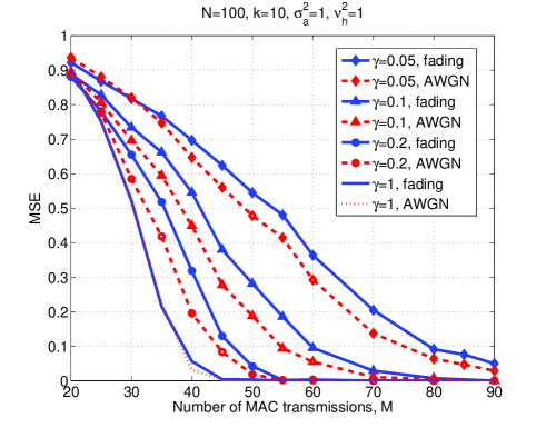
Figure 1: MSE vs number of MAC transmissions with iid fading channels

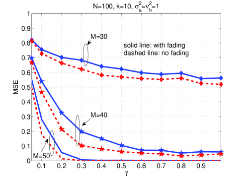
Figure 2: MSE vs measurement sparsity index $\gamma$ with iid fading channels

In Figs. 1 and 2, the MSE vs number of MAC transmissions $M$ and the measurement sparsity index $\gamma$, respectively is plotted for $N=100$, $k=10$, $\sigma_{a}^{2}=1$ and $\nu_{h}^{2}=1$. We further plot the performance in the absence of fading; i.e. assuming AWGN channels so that $\mathbf{B}=\mathbf{A}$. It is observed form both Figs. 1 and 2 that when $\gamma$ is not very small, (i.e. when $\mathbf{B}$ is not very sparse), the impact of fading in recovering a given signal is not significant compared to that with AWGN channels. It is noted that the statistical properties of the measurement matrix changes from light-tailed to heavy-tailed when channels change from AWGN to Rayleigh fading. However, as $M$ and $\gamma$ increase, there is no significant difference in recovery performance with both types of channels. Fig. 2 illustrates the trade-off between $M$ and $\gamma$. It is seen that as $\gamma$ increases beyond $\approx 0.3$, the MSE performance decreases slowly with $\gamma$ for all values of $M$. This corroborates the theoretical results in (27) in which the required number of MAC transmissions that enable recovery of $\mathbf{x}$ based on (6) is proportional to $\frac{1}{\sqrt{\gamma}}$.

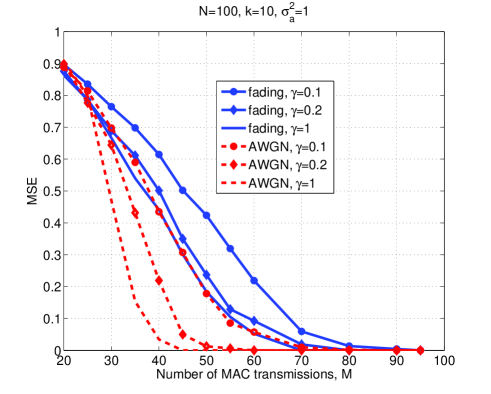
Figure 3: MSE vs number of MAC transmissions with nonidentical fading channels; $\sigma_{a}^{2}=1$, $\nu_{j}\in[1,10]$ for all $j$, $N=100$, $k=10$

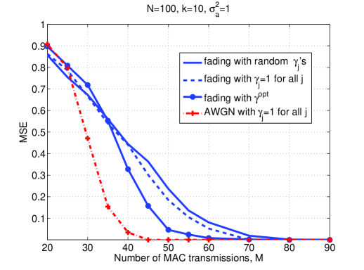
(a) $\nu_{\min}=1$, $\nu_{\max}=10$

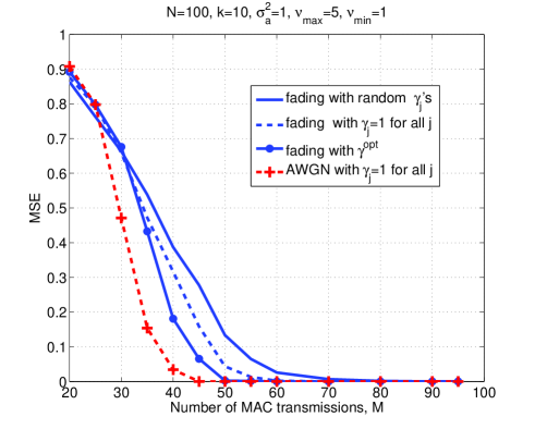
(b) $\nu_{\min}=1$, $\nu_{\max}=5$

Figure 4: MSE vs number of MAC transmissions with nonidentical fading channels; $\sigma_{a}^{2}=1$, $N=100$, $k=10$

V-B Nonidentical fading channels and identical measurement sparsity parameters

Next, we consider the case where fading channels are independent but nonidentical and the measurement sparsity parameter and the power at the each node are the same over all the nodes; i.e. $\gamma_{j}=\gamma$ and $\sigma_{j}^{2}=\sigma_{a}^{2}$ for all $j=0,\cdots,N-1$. Each $\nu_{j}$ is selected uniformly from $[\nu_{\min},\nu_{\max}]$. It is noted that under this case, the elements of the matrix $\mathbf{A}$ are iid but those in $\mathbf{B}$ are non iid. In Fig. 3, we plot the MSE vs $M$. We let $\nu_{\min}=1$, $\nu_{\max}=10$, $k=10$ and $N=100$. In contrast to Fig. 1 with iid fading channels, it can be seen from Fig. 3 that the presence of nonidentical fading channels reduces the capability of sparse recovery quite significantly compared to AWGN channels even when the matrices are dense (i.e. $\gamma=1$). The reason is that, under this case all the nodes transmit with equal probability irrespective of the quality of the fading channels leading to an inhomogeneous measurement matrix. On the other hand, with AWGN, the quality of all the channels is identical and the matrix $\mathbf{A}$ is isotropic. This will be further discussed in the next section.

V-C Nonidentical fading channels and different measurement sparsity parameters

In this section, we consider the case where $\sigma_{j}^{2}=\sigma_{a}^{2}$, and $\nu_{j}$’s are selected uniformly from $[\nu_{\min},\nu_{\max}]$ and arranged in ascending order for $j=0,\cdots,N-1$. The values for $\gamma_{j}$’s are selected as in (24) so that the number of MAC transmissions is minimum with respect to $\bm{\gamma}$. We further assume $\frac{E}{\sigma_{a}^{2}}=1$ so that $\bar{\gamma}=1$ in (24). In Fig. 4, we plot the MSE vs $M$ with $\bm{\gamma}^{\mathrm{opt}}$. We further plot the performance with $\gamma_{j}=1$ for all $j$ considering both AWGN and fading channels. In Fig. 4(a) we let $\nu_{\min}=1$ and $\nu_{\max}=10$ while in Fig. 4(b), we have $\nu_{\min}=1$ and $\nu_{\max}=5$. We make several important observation here. When $\gamma_{j}=1$ and $\sigma_{j}^{2}=\sigma_{a}^{2}$ for all $j$, $\mathbf{A}$ is a iid Gaussian matrix, and $\mathbf{H}$ is a nonidentical (but independent) dense matrix with Rayleigh random variables. In that case, as seen in Fig. 4 , the recovery performance with $\mathbf{B}=\mathbf{A}\odot\mathbf{H}$ (shown in blue dash line) is significantly degraded compared to that with only $\mathbf{A}$ (shown in red marked dash-dot line) due to the inhomogeneity of the matrix $\mathbf{B}$. This corroborates the theoretical results shown in Section III-C. When the matrix $\mathbf{A}$ is made sparse with sparsity parameters as in (24), it can be seen that, recovery performance (blue marked solid line) comparable to AWGN can be achieved especially the ratio $\frac{\nu_{\max}}{\nu_{\min}}$ is small. Further, when the transmission probabilities are selected independent of $\nu_{j}$’s (i.e. randomly) in the presence of nonidentical channel fading, a larger number of MAC transmissions is necessary to achieve negligible MSE compared to having only AWGN channels. When $M$ is small, it is observed that MSE with random $\bm{\gamma}$ is slightly smaller than that with optimal gamma as found in (24). It is worth mentioning that $M$ is optimized over $\bm{\gamma}$ considering perfect signal recovery and this optimality may not hold when $M$ is very small (i.e. in the region where reliable signal recovery is not guaranteed irrespective of $\bm{\gamma}$).

In Figures 1-4, we assumed that the noise power at the fusion center is zero and the recovery is performed based on (6). In Fig. 5, we consider the problem given in (7) where the observations at the fusion center are noisy. Different values for the noise variance $\sigma_{v}^{2}$ are considered and $\epsilon_{v}$ is selected such that $\epsilon_{v}=\sigma_{v}\sqrt{M}\sqrt{1+2\sqrt{2}/\sqrt{M}}$ [33]. As expected, it is observed from Fig. 5 that as $\sigma_{v}^{2}$ increases, the recovery performance is degraded irrespective of the value of $\bm{\gamma}$. However, the use of optimal $\gamma_{j}$, which is obtained in (24) considering the noiseless case, improves the recovery performance even when there is noise compared to the case where each node transmits with arbitrary $\gamma_{j}$ for all $j$.

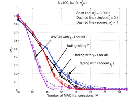
Figure 5: MSE vs number of MAC transmissions with nonidentical fading channels and noise; $\sigma_{a}^{2}=1$, $N=100$, $k=10$, $\nu_{\min}=1$, $\nu_{\max}=10$

VI Conclusion

In this paper, we considered the problem of sparse signal recovery in a distributed sensor network using sparse random matrices. Assuming that the channels between the sensors and the fusion center undergo fading, we derived sufficient conditions that should be satisfied by the number of MAC transmissions to ensure recovery of a given $k$-sparse signal (i.e. for nonuniform recovery). The impact of channel fading makes the corresponding random projection matrix heavy tailed with non identical elements compared to the widely used random matrices in the context of CS which are light tailed (sub-Gaussian). We have exploited the properties of subexponential random matrices with nonidentical elements in deriving nonuniform recovery guarantees under these conditions. We have shown that, when the channels undergo independent and nonidentical fading, by properly designing the probabilities of transmission at each node based on fading channel statistics, the number of measurements required for signal recovery can be reduced. We further provided recovery guarantees of a given sparse signal when the projection matrix is nonidentical sub-exponential in general. An interesting future work is to investigate the impact of channel interference on sparse signal recovery in distributed networks.

Appendix A

Proof of Proposition 1

Let $w=ha$ where we omit the subscripts of $h$ and $a$ for brevity. The pdf of $w$ is given by,

$$f(w)=\int_{-\infty}^{\infty}\frac{h}{\sigma_{h}^{2}}e^{-\frac{h^{2}}{2\sigma_{h}^{2}}}\sqrt{\frac{1}{2\pi\sigma_{a}^{2}}}e^{-\frac{w^{2}}{h^{2}}\frac{1}{2\sigma_{a}^{2}}}\frac{1}{|h|}dh$$ (34)

Since $h\geq 0$, (34) reduces to,

$$f(w)=\sqrt{\frac{1}{2\pi\sigma_{a}^{2}}}\frac{1}{\sigma_{h}^{2}}\int_{0}^{\infty}e^{-\frac{h^{2}}{2\sigma_{h}^{2}}-\frac{w^{2}}{2h^{2}\sigma_{a}^{2}}}dh$$

Using the relation, $\int_{0}^{\infty}e^{-ax^{2}-\frac{b}{x^{2}}}=\frac{1}{2}\sqrt{\frac{\pi}{a}}e^{-2\sqrt{ab}}$ for $a,b>0$, we have,

$$f(w)=\frac{1}{2\bar{\sigma}}e^{-{\frac{1}{\sigma_{h}\sigma_{a}}}|w|}$$

where $\bar{\sigma}=\sigma_{a}\sigma_{h}$, which completes the proof.

Appendix B

Proof of Proposition 2

When the pdf of $u$ is as given in (11), we have,

$$\mathbb{E}\{e^{tu}\} = \int_{-\infty}^{\infty}e^{tu}\left(\gamma_{j}\frac{1}{2\bar{\sigma}_{j}}e^{-\frac{|u|}{\bar{\sigma}_{j}}}+(1-\gamma_{j})\delta(u)\right)du$$

$$= \frac{\gamma_{j}}{2\bar{\sigma}_{j}}\int_{-\infty}^{0}e^{u\left(t+\frac{1}{\bar{\sigma}_{j}}\right)}du$$

$$+ \frac{\gamma_{j}}{2\bar{\sigma}_{j}}\int_{0}^{\infty}e^{u\left(t-\frac{1}{\bar{\sigma}_{j}}\right)}du+(1-\gamma_{j}).$$

When $|t|\leq\frac{1}{\bar{\sigma}_{j}}$, it can be shown that

$$\mathbb{E}\{e^{tu}\}=1+\gamma_{j}\frac{\sigma_{j}^{2}t^{2}}{1-\bar{\sigma}_{j}^{2}t^{2}}.$$ (35)

This holds for any $\bar{\sigma}_{j}$ with $|t|\leq\frac{1}{\underset{j}{\max}\{\bar{\sigma}_{j}\}}$. Thus, when $t^{2}<\frac{1}{\tilde{\eta}_{\max}^{2}}$, based on geometric series formula, we have $\frac{1}{1-\bar{\sigma}_{j}^{2}t^{2}}=\sum_{k=0}^{\infty}(\bar{\sigma}_{j}^{2}t^{2})^{k}$. Thus, (35) can be approximated by,

$$\mathbb{E}\{e^{tu}\} = 1+\gamma_{j}\sum_{k=0}^{\infty}(\bar{\sigma}_{j}^{2}t^{2})^{k+1}$$

$$\approx 1+\gamma_{j}{\sigma_{j}^{2}t^{2}}\leq e^{\gamma_{j}\bar{\sigma}_{j}^{2}t^{2}}\leq e^{\eta_{\max}t^{2}}$$

where $\eta_{\max}=\underset{j}{\max}\{\gamma_{j}\bar{\sigma}_{j}^{2}\}$, completing the proof.

Appendix C

Proof of Proposition 3

Let $\Lambda=\sum_{i=0}^{N-1}\alpha_{i}u_{i}$. Then, using exponential Markov inequality, we have

$$Pr(\Lambda\geq t) = Pr(e^{\lambda\Lambda}\geq e^{\lambda t})\leq e^{-\lambda t}\mathbb{E}\{e^{\lambda\Lambda}\}$$ (36)

$$= e^{-\lambda t}\underset{i}{\prod}\mathbb{E}\{e^{\lambda\alpha_{i}u_{i}}\}.$$

From Proposition 2, we have,

$$Pr(\Lambda\geq t)\leq e^{-\lambda t+\eta_{\max}\lambda^{2}||\bm{\alpha}||_{2}^{2}}$$

when $|\lambda|\leq\frac{1}{\tilde{\eta}_{\max}||\bm{\alpha}||_{\infty}}$. Following similar steps as in the proof of Proposition $5.16$ in [30], we get,

$$Pr(\Lambda\geq t)\leq e^{-\min\left\{\frac{t^{2}}{4\eta_{\max}||\bm{\alpha}||_{2}^{2}},\frac{t}{2\tilde{\eta}_{\max}||\bm{\alpha}||_{\infty}}\right\}}.$$

The same bound is obtained for $Pr(-\Lambda\geq t)$. Thus, we get (13).

Appendix D

Proof of Theorem 1

Proof.

(Theorem 1) We follow similar proof techniques developed for nonuniform recovery with sub-Gaussian matrices in [31] with appropriate modifications to deal with sub-exponential random variables. The failure probability of recovery of $\mathbf{x}$ based on (6) is bounded by

$$P_{e} := Pr(\exists l\notin\mathcal{S}|\langle(\mathbf{B}_{S})^{\dagger}\mathbf{b}_{l},\mathrm{sgn}(\mathbf{x}^{S})\rangle|\geq 1)$$ (37)

$$\leq (N-k)P_{1}^{l}<NP_{1}^{l}$$

where $P_{1}^{l}=Pr(|\langle(\mathbf{B}_{S})^{\dagger}\mathbf{b}_{l},\mathrm{sgn}(\mathbf{x}^{S})\rangle|\geq 1)$.

To bound $P_{1}^{l}$, we use Proposition 3. Conditioned on $\mathbf{B}_{S}$, for given $l$ we have,

$$P_{1}^{l} = Pr(|\langle(\mathbf{B}_{S})^{\dagger}\mathbf{b}_{l},\mathrm{sgn}(\mathbf{x}^{S})\rangle|\geq 1)$$

$$= Pr(|\langle\mathbf{b}_{l},(\mathbf{B}_{S}^{\dagger})^{\star}\mathrm{sgn}(\mathbf{x}^{S})\rangle|\geq 1)$$

$$= Pr\left(|\sum_{j=0}^{M-1}b_{l}(j)[(\mathbf{B}_{\mathcal{S}}^{\dagger})^{*}\mathrm{sgn}(\mathbf{x}^{S})](j)|\geq 1\right)$$

$$\leq 2e^{-\min\left(\frac{1}{4\eta_{\max}||\mathbf{b}_{S}||_{2}^{2}},\frac{1}{2\tilde{\eta}_{\max}||\mathbf{b}_{S}||_{\infty}}\right)}$$

where we define $\mathbf{b}_{S}=(\mathbf{B}_{\mathcal{S}}^{\dagger})^{*}\mathrm{sgn}(\mathbf{x}^{S})$ and $\eta_{\max}$ and $\tilde{\eta}_{\max}$ are as defined in Proposition 2. Thus, we have

$$P_{e}\leq N2e^{-\min\left(\frac{1}{4\eta_{\max}||\mathbf{b}_{S}||_{2}^{2}},\frac{1}{2\tilde{\eta}_{\max}||\mathbf{b}_{S}||_{\infty}}\right)}.$$ (38)

For $P_{e}$ in (38) to be less than $\epsilon$, we have to have,

$$\min\left(\frac{1}{4\eta_{\max}||\mathbf{b}_{S}||_{2}^{2}},\frac{1}{2\tilde{\eta}_{\max}||\mathbf{b}_{S}||_{\infty}}\right)\geq\log(2N/\epsilon).$$ (39)

We can see that (39) is satisfied when,

$$||\mathbf{b}_{S}||_{2}\leq\frac{1}{2\sqrt{\eta_{\max}\log(2N/\epsilon)}}$$

and

$$||\mathbf{b}_{S}||_{\infty}\leq\frac{1}{2\tilde{\eta}_{\max}\log(2N/\epsilon)}.$$

It is noted that $\frac{||\mathbf{b}_{S}||_{\infty}}{||\mathbf{b}_{S}||_{2}}$ is the ratio between peak and total energy of $\mathbf{b}_{S}$ for given $\mathcal{S}$. Let $\frac{||\mathbf{b}_{S}||_{\infty}}{||\mathbf{b}_{S}||_{2}}\leq R$ where $0<R\leq 1$.

Thus, (39) is satisfied when

$$||\mathbf{b}_{S}||_{2}\leq\min\left(\frac{1}{2\sqrt{\eta_{\max}\log(2N/\epsilon)}},\frac{1}{2\tilde{\eta}_{\max}R\log(2N/\epsilon)}\right).$$ (40)

Let $\beta=\min\left(\frac{1}{2\sqrt{\eta_{\max}\log(2N/\epsilon)}},\frac{1}{2\tilde{\eta}_{\max}R\log(2N/\epsilon)}\right)$. To have $Pr(||\mathbf{b}_{S}||_{2}\leq\beta)\geq 1-\epsilon^{\prime}$ for $0<\epsilon^{\prime}<1$, we have to have, $Pr(||\mathbf{b}_{S}||_{2}\geq\beta)\leq\epsilon^{\prime}$. To compute $P_{2}=Pr(||\mathbf{b}_{S}||_{2}\geq\beta)$, we use the following theorem.

Theorem 3 ([30]).

Let $\mathbf{A}$ be a $M\times k$ matrix whose rows $\mathbf{A}_{i}$’s are independent random vectors in $\mathbb{R}^{k}$ with the common second moment matrix $\Sigma=\mathbb{E}\{\mathbf{A}_{i}\otimes\mathbf{A}_{i}\}$. Let $T_{0}$ be a number such that $||\mathbf{A}_{i}||_{2}\leq\sqrt{T_{0}}$ almost surely for all $i$. Then for every $t\geq 0$, the following inequality holds with probability at least $1-ke^{-c^{\prime\prime}t^{2}}$

$$||\frac{1}{M}\mathbf{A}^{T}\mathbf{A}-\Sigma||\leq\max\{||\Sigma||^{1/2}\delta,\delta^{2}\}$$

where $\delta=t\sqrt{\frac{T_{0}}{M}}$ and $c^{\prime\prime}>0$ is an absolute constant. Equivalently, we have,

$$||\Sigma||^{1/2}\sqrt{M}-t\sqrt{T_{0}}\leq s_{\min}(\mathbf{A})\leq s_{\max}(\mathbf{A})$$

$$\leq||\Sigma||^{1/2}\sqrt{M}+t\sqrt{T_{0}}$$ (41)

with probability at least $1-ke^{-c^{\prime\prime}t^{2}}$. Further, when $T_{0}=\mathcal{O}(k)$, (41) reduces to

$$||\Sigma||^{1/2}\sqrt{M}-t\sqrt{k}\leq s_{\min}(\mathbf{A})\leq s_{\max}(\mathbf{A})$$

$$\leq||\Sigma||^{1/2}\sqrt{M}+t\sqrt{k}$$ (42)

with probability at least $1-ke^{-c^{\prime}t^{2}}$ where $c^{\prime}$ is a constant.

Let $\bar{\mathbf{B}}_{S}=\Gamma_{S}\mathbf{B}_{S}$ where $\Gamma_{S}=\sqrt{\frac{k}{\sum_{j=0}^{k-1}2\gamma_{S_{j}}\bar{\sigma}_{S_{j}}^{2}}}$ and $\gamma_{S_{j}}$ (similarly $\bar{\sigma}_{S_{j}}$) corresponds to $\gamma_{i}$ where $i=S_{j}$ is the $j$-th element of $\mathcal{S}$ for $j=0,\cdots,k-1$ and $i$ can take any value from $0,\cdots,N-1$. It is noted that $P_{2}$ can be bounded by

$$P_{2} \leq Pr\left(s_{\min}(\mathbf{B}_{S})\leq\frac{\sqrt{k}}{\beta}\right)$$

$$= Pr\left(s_{\min}(\bar{\mathbf{B}}_{S})\leq\Gamma_{S}\frac{\sqrt{k}}{\beta}\right).$$

Let $\Sigma_{B_{S}}=\mathbb{E}\{(\bar{\mathbf{B}}_{S})_{i}\otimes(\bar{\mathbf{B}}_{S})_{i}\}$ be the second moment matrix of $(\bar{\mathbf{B}}_{S})_{i}$ where $(\bar{\mathbf{B}}_{S})_{i}$ is the $i$-th row of the matrix $\bar{\mathbf{B}}_{S}$. Then, we have $\Sigma_{B_{S}}=\Gamma_{S}^{2}\mathrm{diag}([2\gamma_{S_{0}}\bar{\sigma}^{2}_{S_{0}},\cdots,2\gamma_{S_{k-1}}\bar{\sigma}^{2}_{S_{k-1}}]^{T})$. Since $\mathbf{E}\{||(\bar{\mathbf{B}}_{S})_{i}||_{2}^{2}\}^{1/2}=\sqrt{k}$, we can take $T_{0}=\mathcal{O}(k)$ where $T_{0}$ is a number such that $||(\bar{\mathbf{B}}_{S})_{i}||_{2}\leq\sqrt{T_{0}}$ almost surely for all $i$. Thus, from Theorem 3, we have,

$$Pr\left(s_{\min}(\bar{\mathbf{B}}_{S})\leq||\Sigma_{B_{S}}||^{1/2}\sqrt{M}-t\sqrt{k}\right)\leq ke^{-c^{\prime}t^{2}}$$

where $c^{\prime}$ is a constant. Letting $t=\sqrt{\frac{M}{k}}\left(||\Sigma_{B_{S}}||^{1/2}-\frac{\Gamma_{S}}{\beta}\sqrt{\frac{k}{M}}\right)$, for $P_{2}\leq\epsilon^{\prime}$, it is required that,

$$\frac{M}{k}\left(||\Sigma_{B_{S}}||^{1/2}-\frac{\Gamma_{S}}{\beta}\sqrt{\frac{k}{M}}\right)^{2}\geq\frac{1}{c^{\prime}}\log\left(\frac{k}{\epsilon^{\prime}}\right).$$ (43)

After a simple manipulation, it can be shown that (43) reduces to

$$\sqrt{\frac{M}{k}}\geq\frac{1}{||\Sigma_{B}||^{1/2}}\left(\frac{\Gamma_{S}}{\beta}+\sqrt{\frac{\log(k/\epsilon^{\prime})}{c^{\prime}}}\right).$$ (44)

Using the relations, $\frac{1}{\sqrt{\underset{j}{\max}(2\gamma_{j}\bar{\sigma}_{j}^{2})}}\leq\Gamma_{S}\leq\frac{1}{\sqrt{\underset{j}{\min}(2\gamma_{j}\bar{\sigma}_{j}^{2})}}$ and $||\Sigma_{B}||^{1/2}\geq\sqrt{\frac{\underset{j}{\min}(2\gamma_{j}\bar{\sigma}_{j}^{2})}{\underset{j}{\max}(2\gamma_{j}\bar{\sigma}_{j}^{2})}}$, (44) is satisfied when

$$\sqrt{\frac{M}{k}}\geq\sqrt{\frac{\eta_{\max}}{\eta_{\min}}}\left(\frac{1}{\beta\sqrt{2\eta_{\min}}}+\sqrt{\frac{\log(k/\epsilon^{\prime})}{c^{\prime}}}\right)$$ (45)

where we define $\eta_{\max}=\underset{j}{\max}(\gamma_{j}\bar{\sigma}_{j}^{2})$ and $\eta_{\min}=\underset{j}{\min}(\gamma_{j}\bar{\sigma}_{j}^{2})$. When $\beta=\frac{1}{2\sqrt{\eta_{\max}\log(2N/\epsilon)}}$, (45) reduces to,

$$M\geq\frac{\eta_{\max}}{\eta_{\min}}k\left(\sqrt{\frac{2\eta_{\max}}{\eta_{\min}}}\sqrt{\log(2N/\epsilon)}+\sqrt{\frac{\log(k/\epsilon^{\prime})}{c^{\prime}}}\right)^{2}$$

On the other hand, when $\beta=\frac{1}{2\tilde{\eta}_{\max}R\log(2N/\epsilon)}$, we have,

$$M\geq{\frac{\eta_{\max}}{\eta_{\min}}}k\left(\frac{\sqrt{2}\tilde{\eta}_{\max}}{\sqrt{\eta_{\min}}}R\log(2N/\epsilon)+\sqrt{M}\sqrt{\frac{\log(k/\epsilon^{\prime})}{c^{\prime}}}\right)^{2}$$

completing the proof. ∎

Appendix E

We have

$$||\mathbf{b}_{S}||_{2}^{2} = (\mathrm{sgn}(\mathbf{x}^{S}))^{T}(\mathbf{B}_{S}^{T}\mathbf{B}_{S})^{-1}\mathrm{sgn}(\mathbf{x}^{S})$$

$$\approx \frac{1}{M}\underset{j\in\mathcal{S}}{\sum}\frac{1}{2\gamma_{j}\bar{\sigma}_{j}^{2}}$$

with sufficiently large $M$. Thus,

$$||\mathbf{b}_{S}||_{2}\geq\sqrt{\frac{k}{2M\eta_{\max}}}.$$

With sufficiently large $M$, the $i$-th element of $\mathbf{b}_{S}$ can be approximated by,

$$\mathbf{b}_{S}(i)\approx\frac{1}{M}\sum_{j=0}^{k-1}\frac{(\mathbf{B}_{S})_{ij}}{2\gamma_{S_{j}}\bar{\sigma}_{S_{j}}^{2}}\mathrm{sgn}(\mathbf{x}^{S})(j).$$

Thus, we have,

$$|\mathbf{b}_{S}(i)| \leq \frac{1}{M}\sum_{j=0}^{k-1}\frac{|(\mathbf{B}_{S})_{ij}|}{2\gamma_{S_{j}}\bar{\sigma}_{S_{j}}^{2}}.$$

It is noted that $\mathbb{E}\{|(\mathbf{B}_{S})_{ij}|\}=\gamma_{S_{j}}\bar{\sigma}_{S_{j}}$. Thus,

$$\mathbb{E}\{|\mathbf{b}_{S}(i)|\} \leq \frac{1}{M}\sum_{j=0}^{k-1}\frac{1}{2\bar{\sigma}_{S_{j}}}$$

$$\leq \frac{k}{2M\tilde{\eta}_{\min}}$$

where $\tilde{\eta}_{\min}=\underset{j}{\min}\{\bar{\sigma}_{j}\}$. Then we have,

$$\mathbb{E}\left\{\frac{||\mathbf{b}_{S}||_{\infty}}{||\mathbf{b}_{S}||_{2}}\right\}\leq\frac{\sqrt{k\eta_{\max}}}{\sqrt{2M\tilde{\eta}_{\min}^{2}}}\leq\frac{\sqrt{k}}{\sqrt{2M}}.$$

Thus, $R$ can be considered to be

$$R=\mathcal{O}\left(\sqrt{\frac{k}{2M}}\right).$$

Appendix F

Proof of Theorem 2

We follow a similar approach as in the proof of Theorem 1 in Appendix D. For a given support set $\mathcal{S}$, the failure probability in recovering $\mathbf{x}$ from (6) is upper bounded by,

$$P_{e}\leq NP_{l}$$ (46)

where $P_{l}=Pr(|\langle(\mathbf{B}_{S})^{\dagger}\mathbf{b}_{l},\mathrm{sgn}(\mathbf{x}^{S})\rangle|\geq 1)$. Using Proposition 5.16 in [30], $P_{l}$ can be upper bounded by,

$$P_{l}\leq 2e^{-c_{1}\min\left(\frac{1}{\rho_{\max}^{2}||\mathbf{b}_{S}||_{2}^{2}},\frac{1}{\rho_{\max}||\mathbf{b}_{S}||_{\infty}}\right)}$$

where $c_{1}$ is a constant and $\mathbf{b}_{S}=(\mathbf{B}_{S}^{\dagger})^{*}\mathrm{sgn}(\mathbf{x}^{S})$ as defined in Appendix D. Then, $P_{e}$ in (46) can be bounded above by $\epsilon_{1}$ if

$$\min\left(\frac{1}{\rho_{\max}^{2}||\mathbf{b}_{S}||_{2}^{2}},\frac{1}{\rho_{\max}||\mathbf{b}_{S}||_{\infty}}\right)\geq\frac{1}{c_{1}}\log(2N/\epsilon_{1}).$$ (47)

Let the matrix $\mathbf{B}$ be such that for any given $\mathcal{S}$, $\frac{||\mathbf{b}_{S}||_{\infty}}{||\mathbf{b}_{S}||_{2}}\leq R_{1}$ almost surely where $0<R_{1}<1$. Then, (47) is satisfied when,

$$||\mathbf{b}_{S}||_{2}\leq\min\left(\frac{1}{\rho_{\max}}\sqrt{\frac{c_{1}}{\log(2N/\epsilon_{1})}},\frac{c_{1}}{\rho_{\max}R_{1}\log(2N/\epsilon_{1})}\right)$$ (48)

Let $\beta_{1}=\min\left(\frac{1}{\rho_{\max}}\sqrt{\frac{c_{1}}{\log(2N/\epsilon_{1})}},\frac{c_{1}}{\rho_{\max}R_{1}\log(2N/\epsilon_{1})}\right)$. We have,

$$Pr(||\mathbf{b}_{S}||_{2}\geq\beta_{1})\leq Pr\left(s_{\min}(\mathbf{B}_{S})\leq\frac{\sqrt{k}}{\beta_{1}}\right).$$

Using the Theorem 3, we get,

$$Pr(s_{\min}(\mathbf{B}_{S})\leq||\Sigma_{\mathbf{B}_{S}}||^{1/2}\sqrt{M}-t\sqrt{T_{0}})\leq ke^{-c^{\prime}_{1}t^{2}}$$

where $T_{0}$ is a number such that $||(\mathbf{B}_{S})_{i}||_{2}\leq\sqrt{T_{0}}$ for all $i$ and $c^{\prime}_{1}$ is a constant. Letting $t=\sqrt{\frac{M}{T_{0}}}\left(||\Sigma_{\mathbf{B}_{S}}||^{1/2}-\frac{\sqrt{k}}{\beta_{1}\sqrt{M}}\right)$, it can be shown that $Pr(||\mathbf{b}_{S}||_{2}\geq\beta_{1})\leq\epsilon_{1}^{\prime}$ when

$$M\geq\frac{1}{||\Sigma_{\mathbf{B}_{S}}||}\left(\frac{\sqrt{k}}{\beta_{1}}+\sqrt{\frac{T_{0}\log(k/\epsilon^{\prime}_{1})}{c_{1}}}\right)^{2}.$$ (49)

Thus, (49) is satisfied when,

$$M\geq\frac{1}{\lambda_{\min}}\left(\frac{\sqrt{k}}{\beta_{1}}+\sqrt{\frac{T_{0}\log(k/\epsilon^{\prime}_{1})}{c^{\prime}_{1}}}\right)^{2}$$

where $\lambda_{\min}$ is the minimum eigenvalue of $\Sigma_{B}^{T}\Sigma_{B}$ completing the proof.

References

• [1] J. Haupt, W. U. Bajwa, M. Rabbat, and R. Nowak, “Compressed sensing for networked data,” IEEE Signal Processing Magazine, pp. 92–101, Mar. 2008.
• [2] W. Wang, M. Garofalakis, and K. Ramchandran, “Distributed sparse random projections for refinable approximation,” in ISPN, Cambridge, Massachusetts,USA, April 2007, pp. 331–339.
• [3] Y. Shen, W. Hu, R. Rana, and C. T. Chou, “Nonuniform compressive sensing for heterogeneous wireless sensor networks,” IEEE Sensors journal, pp. 2120–2128, June 2013.
• [4] G. Yang, V. Y. F. Tan, C. K. Ho, S. H. Ting, and Y. L. Guan, “Wireless compressive sensing for energy harvesting sensor nodes,” IEEE Trans. Signal Processing, vol. 61, no. 18, pp. 4491–4505, Sept. 2013.
• [5] D. Baron, M. Duarte, S. Sarvotham, M. B. Wakin, and R. G. Baraniuk, “Distributed compressed sensing,” Rice Univ. Dept. Elect. Comput. Eng. Houston, TX, Tech. Rep. TREE 0612, Nov 2006.
• [6] Q. Ling and Z. Tian, “Decentralized sparse signal recovery for compressive sleeping wireless sensor networks,” IEEE Trans. Signal Processing, vol. 58, no. 7, pp. 3816–3827, July 2010.
• [7] C. Caione, D. Brunelli, and L. Benini, “Distributed compressive sampling for lifetime optimization in dense wireless sensor networks,” IEEE Trans. Industrial Informatics, vol. 1, no. 8, pp. 30–40, Feb 2012.
• [8] M. Sartipi and R. Fletcher, “Energy-efficient data acquisition in wireless sensor networks using compressed sensing,” in Data Compression Conference (DCC), 2011, pp. 223–232.
• [9] T. Wimalajeewa and P. K. Varshney, “Cooperative sparsity pattern recovery in distributed networks via distributed-OMP,” in Proc. Acoust., Speech, Signal Processing (ICASSP), Vancouver, Canada, May 2013.
• [10] ——, “OMP based joint sparsity pattern recovery under communication constraints,” IEEE Trans. Signal Processing, vol. 62, no. 9, pp. 5059–5072, Oct. 2014.
• [11] Y. Zheng, T. Wimalajeewa, and P. K. Varshney, “Probabilistic sensor management for target tracking via compressive sensing,” in Proc. Acoust., Speech, Signal Processing (ICASSP), Florence, Italy, May 2014.
• [12] F. Fazel, M. Fazel, and M. Stojanovic, “Random access compressed sensing over fading and noisy communication channels,” IEEE Trans. Wireless Commun., vol. 12, no. 5, pp. 2114–2125, May 2013.
• [13] S. Colonnese, R. Cusani, S. Rinauro, G. Ruggiero, and G. Scarano, “Efficient compressive sampling of spatially sparse fields in wireless sensor networks,” EURASIP Journal on Advances in Signal Processing, p. 19 pages, 2013.
• [14] D. Achlioptas, “Database-friendly random projections: Johnson-lindenstrauss with binary coins,” Journal of Computer and System Sciences, vol. 66, no. 4, pp. 671–687, 2003.
• [15] W. Wang, M. J. Wainwright, and K. Ramachandran, “Information-theoretic limits on sparse signal recovery: Dense versus sparse measurement matrices,” IEEE Trans. Inform. Theory, vol. 56, no. 6, pp. 2967–2979, Jun. 2010.
• [16] A. Gilbert and P. Indyk, “Sparse recovery using sparse matrices,” Proc. IEEE, vol. 98, no. 6, pp. 937–947, 2010.
• [17] P. Li, T. Hastie, and K. Church, “Very sparse random projections,” in Proceedings of the 12th ACM SIGKDD international conference on Knowledge discovery and data mining (KDD), April 2006, pp. 287–296.
• [18] E. Cand$\grave{e}$s, J. Romberg, and T. Tao, “Stable signal recovery from incomplete and inaccurate measurements,” Communications on Pure and Applied Mathematics, vol. 59, no. 8, pp. 1207–1223, Aug. 2006.
• [19] D. Donoho, “Compressed sensing,” IEEE Trans. Inform. Theory, vol. 52, no. 4, pp. 1289–1306, Apr. 2006.
• [20] E. J. Candès and Y. Plan, “A probabilistic and ripless theory of compressed sensing,” IEEE Trans. Inform. Theory, vol. 57, no. 11, pp. 7235–7254, 2011.
• [21] Y. C. Eldar and G. Kutyniok, Compressed Sensing: Theory and Applications.   Cambridge University Press, 2012.
• [22] H. Rauhut, “Compressive sensing and structured random matrices,” In M. Fornasier, editor, Theoretical Foundations and Numerical Methods for Sparse Recovery, of Radon Series Comp. Appl. Math. deGruyter, vol. 9, 2010.
• [23] K. Cohen and A. Leshem, “Performance analysis of likelihood-based multiple access for detection over fading channels,” IEEE Trans. Information Theory, vol. 59, no. 4, pp. 2471–2481, Apr. 2013.
• [24] Y. Chen, Q. Zhao, V. Krishnamurthy, and D. Djonin, “Transmission scheduling for optimizing sensor network lifetime: A stochastic shortest path approach,” IEEE Trans. Signal Processing, vol. 55, no. 5, pp. 2294–2309, May 2007.
• [25] W. U. Bajwa, J. D. Haupt, A. M. Sayeed, and R. D. Nowak, “Joint source-channel communication for distributed estimation in sensor networks,” IEEE Trans. Information Theory, vol. 53, no. 10, pp. 3629–3653, Oct. 2007.
• [26] M. Gastpar, B. Rimoldi, and M. Vetterli, “To code, or not to code: Lossy source-channel communication revisited,” IEEE Trans. Information Theory, vol. 49, pp. 1147–1158, May 2003.
• [27] M. Gastpar, “Uncoded transmission is exactly optimal for a simple gaussian sensor network,” IEEE Trans. Information Theory, vol. 54, no. 11, pp. 5247–5251, Nov. 2008.
• [28] G. Mergen and L. Tong, “Type based estimation over multiaccess channels,” IEEE Trans. Signal Processing, vol. 54, no. 2, pp. 613–626, Feb. 2006.
• [29] S. Marano, V.Matta, L. Tong, and P.Willett, “A likelihood-based multiple access for estimation in sensor networks,” IEEE Trans. Signal Processing, vol. 55, no. 11, pp. 5155–5166, Nov. 2007.
• [30] R. Vershynin, Introduction to the non-asymptotic analysis of random matrices. In Compressed Sensing: Theory and Applications, Y. Eldar and G. Kutyniok, Eds.   Cambridge University Press., 2010.
• [31] U. Ayaz and H. Rauhut, “Nonuniform sparse recovery with subgaussian matrices,” in Technical Report, University of Bonn, Germany, 2011.
• [32] J.-J. Fuchs, “On sparse representations in arbitrary redundant bases,” IEEE Trans. Inform. Theory, vol. 50, pp. 1341–1344, 2004.
• [33] E. Candes and J. Romberg, “l1-magic: Recovery of sparse signals via convex programming,” http://www.acm.caltech.edu/l1magic/, 2005.