From Canards of Folded Singularities to
Torus Canards in a Forced van der Pol Equation

Abstract

In this article, we study canard solutions of the forced van der Pol equation in the relaxation limit for low-, intermediate-, and high-frequency periodic forcing. A central numerical observation made herein, which motivated our study, is that there are two branches of canards in parameter space which extend across all positive forcing frequencies. In the low-frequency forcing regime, we demonstrate the existence of the primary maximal canards induced by folded saddle-nodes of type I, and establish explicit formulas for the parameter values at which the primary maximal canards and their fold curves exist. Then, we turn to the intermediate- and high-frequency forcing regimes, and show that the forced van der Pol possesses torus canards instead. These torus canards consist of long segments near families of attracting and repelling limit cycles of the fast system, in alternation. We also derive explicit formulas for the parameter values at which the maximal torus canards and their fold curves exist. Primary maximal canards and maximal torus canards correspond geometrically to the situation in which the persistent manifolds near the family of attracting limit cycles coincide to all orders with the persistent manifolds that lie near the family of repelling limit cycles. The formulas derived for the folds of maximal canards in all three frequency regimes turn out to be representations of a single formula in the appropriate parameter regimes, and this unification confirms the central numerical observation that the folds of the maximal canards created in the low-frequency regime continue directly into the fold curves of the maximal torus canards that exist in the intermediate- and high-frequency regimes. In addition, we study the secondary canards induced by the folded singularities in the low-frequency regime and find that the fold curves of the secondary canards turn around in the intermediate-frequency regime, instead of continuing into the high-frequency regime as the primary maximal canards do. Also, we identify the mechanism responsible for this turning. Finally, we show that the forced van der Pol equation is a normal form type equation for a class of single-frequency periodically-driven slow/fast systems with two fast variables and one slow variable which possess a nondegenerate fold of limit cycles. The analytic techniques used herein rely on geometric desingularization, invariant manifold theory, Melnikov theory, and normal form methods. The numerical methods used herein were developed in [13, 14].

Keywords folded singularities, canards, torus canards, torus bifurcation, mixed-mode oscillations

AMS subject classifications Primary: 34E17, 34E15, 34D26, 70K70; Secondary: 34E13, 34D15, 34C29, 34C45, 37G15, 92C20, 70K43

1 Introduction

The forced van der Pol equation is a fundamental model for oscillatory processes in physics, electronics, biology, neurology, sociology, and economics. Possessing strong nonlinear damping effects, it is the prototype of a forced relaxation oscillator, exhibiting slow and fast time scales, see [5, 9, 10, 24, 29, 30, 39, 40, 50, 43, 45]. The equations may be formulated as

$$\begin{split}x^{\prime}&=y-f(x),\\ y^{\prime}&=\operatorname{\varepsilon}(-x+a+b\cos\theta),\\ \theta^{\prime}&=\omega,\end{split}$$ (1)

where the prime denotes the derivative with respect to the fast time variable $\tau$, $f(x)=\frac{1}{3}x^{3}-x$, and $0<\operatorname{\varepsilon}\ll 1$. The external signal, $a+b\cos\theta$, models a time-periodic driving force with drive frequency $\omega>0$. We refer to equation (1) as the fvdP equation. Throughout this article, we will work with the form of the system given by (1), as it allows us to explore the full range of forcing frequencies $\omega>0$.

A number of detailed studies of forced van der Pol equations have been carried out in the low-frequency forcing regime, $\omega=\mathcal{O}(\operatorname{\varepsilon})$, see [5, 27, 30, 52]. We cite in particular the study [5] of a forced van der Pol system with low-frequency forcing, which presents a detailed analysis of the folded saddle singularities and their attendant canards. In the context of excitable systems (in particular, neuronal models), the folded saddle maximal canard plays the role of an excitability threshold manifold, locally dividing trajectories between those that jump at the fold to a different attracting manifold and those that do not [42, 57]. This is also true in planar neuronal systems where solutions containing maximal canard segments correspond to excitability thresholds both in the case of type I neurons (integrators) and type II neurons (resonators) [16, 31]. More generally, the canards induced by folded singularities, of folded node, folded saddle, and folded saddle-node types, have also been studied in models of neuronal dynamics [47, 48, 53] and in many other systems, see for example [4, 7, 13, 15, 37, 54, 55, 56, 57].

In this article, we examine the fvdP equation (1) in three different regimes of forcing frequencies: low-frequency ($\omega={\cal O}(\operatorname{\varepsilon})$), intermediate-frequency ($\omega={\cal O}(\sqrt{\operatorname{\varepsilon}})$), and high-frequency ($\omega={\cal O}(1)$). In each regime, we study the canard solutions that the fvdP equation (1) exhibits.

We begin in the low-frequency regime. First, we briefly apply the theory of folded singularities to (1), to identify the different types of folded singularities that it exhibits in this regime. We place special emphasis on folded saddle-node singularities of type I (FSN I), which are known to generate a number of different types of canard solutions.

The graph of the fast null-cline, $y=f(x)$, of system (1) with $\operatorname{\varepsilon}=0$ plays a central role in understanding the system dynamics. We are especially interested in the repelling branch in the middle and the attracting branch on the right, respectively, of the graph. Let $S_{r}$ denote the two-dimensional manifold formed by rotating the (middle) repelling branch through one complete revolution in the angle $\theta:[0,2\pi)$, and similarly let $S_{a}$ be the the two-dimensional manifold formed by rotating the (right) attracting branch through one complete revolution in $\theta$. In the low-frequency regime of (1), Fenichel theory [23, 33] guarantees that, when $\operatorname{\varepsilon}$ is sufficiently small, there exist two-dimensional, locally-invariant manifolds $S_{r}^{\operatorname{\varepsilon}}$ and $S_{a}^{\operatorname{\varepsilon}}$ near $S_{r}$ and $S_{a}$, respectively, away from the fold regions. In the low-frequency forcing regime of (1), these persistent manifolds are referred to as slow manifolds, since the dynamics on them is slow in $y$ and $\theta$.

The primary canards of folded singularities are orbits that have a long segment close to $S_{a}^{\operatorname{\varepsilon}}$, pass through a neighborhood of the folded singularity, and then have a long segment near $S_{r}^{\operatorname{\varepsilon}}$. The lengths of these segments depend on the parameter values; and, there are curves of parameter values along which the segment near $S_{r}^{\operatorname{\varepsilon}}$ has maximal length, going all the way up to the other fold curve. These primary canards are referred to as primary maximal canards. See Figure 1(a) for a representative primary maximal canard. They are determined geometrically by the parameter values for which $S_{r}^{\operatorname{\varepsilon}}$ and $S_{a}^{\operatorname{\varepsilon}}$ agree to all orders in $\operatorname{\varepsilon}$, in a manner that is analogous to the maximal limit cycle canards (also known as the maximal headless ducks) in the classical, planar van der Pol equation, recall [3, 17, 21].

The following is the first main result of this article:

Theorem 1.1.

low-frequency forcing. Let $\omega=\operatorname{\varepsilon}\overline{\omega}$, where $\overline{\omega}={\cal O}(1)$, and let $b=\mathcal{O}(\sqrt{\operatorname{\varepsilon}})$. Then, there exists an $\operatorname{\varepsilon}_{0}>0$ such that for all $0<\operatorname{\varepsilon}<\operatorname{\varepsilon}_{0}$, there are two curves in the $(a,\overline{\omega})$ parameter plane given by

$$a=1-\frac{\operatorname{\varepsilon}}{8}\pm b\exp\left(-\frac{\operatorname{\varepsilon}\overline{\omega}^{2}}{2}\right),$$ (2)

emanating from the points $(\overline{\omega},a)=(0,1-\frac{\operatorname{\varepsilon}}{8}\pm b)$, along which the system (1) has folds of primary maximal canards. Moreover, for each ${\cal O}(1)$ value of $\overline{\omega}$, the system (1) has two primary maximal canards for every value of $a$ in the interval between the points on these fold curves. Finally, there are no primary maximal canards for values of $a$ outside the closures of these intervals.

This first theorem is established by using the geometric desingularization method, also known as the blow-up method [19, 20, 36], to inflate the folded saddle node points of type I into hyperspheres, and then by employing invariant manifold theory and Melnikov theory in the appropriate coordinate charts.

Next, we show that the fvdP system (1) has torus canards in both the regime of intermediate-frequency forcing, in which the system (1) has three time scales: $x$ is a fast variable, $\theta$ is an intermediate time variable, and $y$ is a slow variable; and in the regime of high-frequency forcing in which (1) is a two-fast ($x,\theta$) and one-slow system ($y$). Torus canards are a relatively new type of canard solution discovered in a model of neuronal activity in Purkinje cells [34]. They consist of long segments near families of attracting and repelling limit cycles of the fast system, in alternation. Torus canards have recently been shown to exist in a broad array of models, including in three models of neuronal bursting, see [8]: the Hindmarsh-Rose model, the Morris-Lecar-Terman system, and the Wilson-Cowan-Izhikevich equations; in a model of elliptic bursters, where the torus canards are rotated versions of limit cycle canards of a planar system, see [32]; in a rotated van der Pol-type model system, see [2]; as well as more recently in a model of respiratory rhythm generation in a pre-Bötzinger complex, see [46]. The significance of torus canards is that they play a central role in the transition between periodic spiking and bursting, of different types, in these neuronal models.

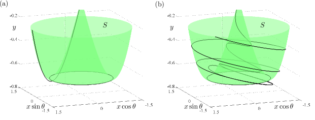
Figure 1: (a) Segment of a primary maximal canard solution of (1), and (b) segment of a maximal torus canard solution of (1). Both have long segments near the family of attracting limit cycles (outer portion of the green surface) and near the family of repelling limit cycles (inner portion of the green surface). Here, $a=0.997,b=0.994,\operatorname{\varepsilon}=0.02$, and (a) $\omega=0.001$ and (b) $\omega=0.3$.

In the intermediate- and high-frequency regimes of (1), Fenichel theory [23, 33] also guarantees that, when $\operatorname{\varepsilon}$ is sufficiently small, there exist two-dimensional, locally-invariant manifolds near $S_{r}$ and $S_{a}$, away from the fold regions. We again denote these by $S_{r}^{\operatorname{\varepsilon}}$ and $S_{a}^{\operatorname{\varepsilon}}$ and label them as persistent manifolds. However, it is crucial to observe that these persistent manifolds are no longer slow manifolds in these regions. Instead, the orbits of (1) on these persistent manifolds exhibit two time scales, with fast rotation due to the limit cycles, as well as slow drift in the vertical direction, down $S_{a}^{\operatorname{\varepsilon}}$ and up along $S_{r}^{\operatorname{\varepsilon}}$.

Torus canards are orbits of (1) in the intermediate- and high-frequency regimes that have long segments near $S_{a}^{\operatorname{\varepsilon}}$, spiral through a neighborhood of the fold curve of limit cycles, and then have a long segment near $S_{r}^{\operatorname{\varepsilon}}$. The lengths of time that torus canards spiral around near $S_{a}^{\operatorname{\varepsilon}}$ and $S_{r}^{\operatorname{\varepsilon}}$ depend on the system parameters, and for system (1) there are curves of parameter values along which the time spent near $S_{r}^{\operatorname{\varepsilon}}$ is maximal, with the orbits spiralling all the way up $S_{r}^{\operatorname{\varepsilon}}$. These are defined to be maximal torus canards, in analogy with the maximal limit cycle canards of the unforced van der Pol oscillator. A representative maximal torus canard is shown in Figure 1(b).

For system (1) in the intermediate-frequency regime, we prove the following theorem:

Theorem 1.2.

intermediate-frequency forcing. Let $\omega=\sqrt{\operatorname{\varepsilon}}\Omega$, where $\Omega={\cal O}(1)$, and let $b=\mathcal{O}(\operatorname{\varepsilon})$. Then, there exists an $\operatorname{\varepsilon}_{0}>0$ such that for all $0<\operatorname{\varepsilon}<\operatorname{\varepsilon}_{0}$, there are two curves in the $(a,\Omega)$ parameter plane given by

$$a=1-\frac{\operatorname{\varepsilon}}{8}\pm b\exp\left(-\frac{\Omega^{2}}{2}\right).$$ (3)

along which the system (1) has folds of maximal canards. Moreover, for each fixed ${\cal O}(1)$ value of $\Omega$, the system (1) has two canards for every value of $a$ in the interval between these fold curves, and none outside the closure of these intervals.

This theorem is also established by using the geometric desingularization method; however, in this regime, we inflate the circular fold curve along which the attracting and repelling limit cycles meet into a two-torus, rather than the FSN I points. Also, the scalings are different, as is the analysis in the coordinate charts near the torus.

Then, for the high-frequency regime, we establish:

Corollary 1.3.

high-frequency forcing. Let $\omega={\cal O}(1)$, and let $b=\mathcal{O}(\operatorname{\varepsilon})$. Then, there exists an $\operatorname{\varepsilon}_{0}>0$ such that for all $0<\operatorname{\varepsilon}<\operatorname{\varepsilon}_{0}$, there are two curves in the $(a,\omega)$ parameter plane given by

$$a=1-\frac{\operatorname{\varepsilon}}{8}\pm b\exp\left(-\frac{\omega^{2}}{2\operatorname{\varepsilon}}\right).$$ (4)

along which the system (1) has folds of torus canards. Moreover, there exists a pair of torus canards for each parameter value in the interval between these fold curves.

We note that the presence of the torus canards in this type of fast-slow system is signalled by the existence of a fold of limit cycles of the fast system, here at $(x,y)=(1,-\frac{2}{3})$, together with a nearby torus bifurcation in the full system, here at

$$1-a^{2}-\frac{1}{2}\frac{b^{2}\operatorname{\varepsilon}^{2}}{(a^{2}-1)^{2}\omega^{2}+(\operatorname{\varepsilon}-\omega^{2})^{2}}=0.$$ (5)

See Appendix A. These two triggering mechanisms arise ubiquitously in fast-slow systems with two or more fast variables.

Having established these theorems for the existence of the primary maximal canards and the torus canards, as well as their folds, we now analyze the relationship between these results. Plainly, the formulas for the curves of folds (2), (3), and (4) in the three different regimes are all representations of the same formula,

$$a=1-\frac{\operatorname{\varepsilon}}{8}\pm b\exp\left(-\frac{\omega^{2}}{2\operatorname{\varepsilon}}\right),$$ (6)

in the respective frequency regimes. The exponential term has magnitude $b$ (which is ${\cal O}(\sqrt{\operatorname{\varepsilon}}))$ and is slowly varying with $\overline{\omega}$ in the low-frequency regime (Theorem 1.1), small-amplitude ($b=\mathcal{O}(\operatorname{\varepsilon})$) and varying with ${\cal O}(1)$ frequency $\Omega$ in the intermediate-frequency regime (Theorem 1.2), and exponentially small in $\operatorname{\varepsilon}$ in the high-frequency regime (Corollary 1.3).

Figure 2: Curves of folds of maximal canards in the $(\omega,a)$ plane as obtained from (6) (red curves) and 2-parameter numerical continuation (blue curves) for $\operatorname{\varepsilon}=0.01$ and (a) $b=0.01$; (b) $b=0.02$; (c) $b=0.035$l and, (d) $b=0.1$. For $b=\mathcal{O}(\operatorname{\varepsilon})$ (panels (a)–(c)), there is good agreement between theoretical (red) and numerical (blue) results over the entire range of forcing frequencies, including for both the primary maximal canards which exist for $\omega={\cal O}(\operatorname{\varepsilon})$ and the maximal torus canards which exist for $\omega={\cal O}(1)$. Note that the scales in panels (a)–(c) are the same. For $b=\mathcal{O}(\sqrt{\operatorname{\varepsilon}})$ (panel (d), in which the vertical scale is different), we find that the numerical continuation terminates when $\omega$ is no longer $\mathcal{O}(\operatorname{\varepsilon})$.

The analysis in all three regions shows that the values of the parameter $a$ for which the canards exist in between the fold curves may similarly be summarized succinctly in one formula:

$$a=1-\frac{\operatorname{\varepsilon}}{8}-b\cos(\theta_{0})\exp\left(-\frac{\omega^{2}}{2\operatorname{\varepsilon}}\right).$$ (7)

Here, $\theta_{0}$ is an arbitrary phase, and the magnitude and dynamics of the exponential term are also as discussed above.

It is also of interest to observe that, in the limit of $\omega\to\infty$, formulas (6) and (7) become $a\to a_{c}:=1-\frac{\operatorname{\varepsilon}}{8}$, which corresponds exactly to the leading order locations of the maximal limit cycle canards in the planar vdP equation, see for example [36]. Therefore, as expected, for sufficiently high-frequency forcing, the effect of the forcing averages out to this order, and (1) behaves like the classical planar vdP equation. In this limiting regime, the torus canards of (1) appear to be rotated copies of the limit cycle canards of the planar vdP.

Then, with the above analytical results in hand, we turn next to the results of numerical continuations which confirm that the curves of the folds of primary strong canards observed in the low-frequency regime continue directly to the curves of the folds of torus canards discovered in the intermediate- and high-frequency regimes. This is illustrated in Figure 2. Moreover, as is also shown in this figure, the agreement between the formulas and the numerical continuation results are excellent within the parameter regions stated in the theorems. We also note that the theory does not appear to extend outside of these regions, and also preliminary results of numerical continuation reveal different dynamics there. Overall, then, the formulas (6), and (7) together with the numerical continuations, will directly imply that the primary strong canards, which exist in the low-frequency forcing region, continue naturally to the branches of torus canards, which exist in the high-frequency regime, where the folded singularities cease to exist, with the transition happening in the intermediate-frequency regime. Understanding the continuation dynamics of these curves is one of the main results of this article. Moreover, the results here will also help shed light on other models with torus canards. In particular, we observe that numerical simulations of a rotated van der Pol-type model exhibit the same continuation of the maximal canards across the entire range of forcing frequencies; see Figure 5 in [2]. Numerical continuations in other neuronal (or neural) models [8] show similar phenomena.

In this article, we also study the secondary canards of (1). Secondary canards, lie near the primary canards for most of their lengths, and make a number of small loops around an axis of rotation usually referred to as the weak canard. Secondary canards are indexed by the number of loops they make around the weak canard and by the value of the $y$-intercepts of the solutions during the nearly-horizontal jumps that occur from a neighborhood of the family of repelling limit cycles back to a neighborhood of the family of attracting limit cycles. In particular, we carry out numerical continuation of the branches of maximal secondary canards of (1) that are created by the folded singularities in the low-frequency regime. In contrast to what we find for the primary canards, the branches of the secondary canards turn around well before they reach the high-frequency regime. See Figure 3. Also, we identify the mechanisms which cause the branches to turn.

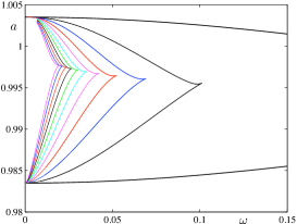
Figure 3: Curves of folds along the computed branches of primary and secondary canards. Here, $\operatorname{\varepsilon}=0.05$ and $b=0.01$.

To conclude this article, we demonstrate that (1) serves as a local normal form for slow/fast systems with one slow variable and two fast variables in which the fast subsystem possesses a non-degenerate fold of limit cycles, and in which the slow system is subject to time-periodic forcing. These fast-slow systems exhibit torus canard explosions, just as shown here for the fvdP equation (1), and one may therefore directly conclude, by applying the same techniques used herein, that the folds of their canards behave in a similar fashion.

Figure 4: 2-parameter continuation of folds of primary maximal canards of a folded saddle-node (type I) for $\operatorname{\varepsilon}=0.01$ and $b=0.01$. Orbit segments are plotted in ‘Cartesian’ coordinates $(u,v,y)=(x\cos\theta,x\sin\theta,y)$.

The numerical method developed in [13, 14], and also employed in [15], is the main numerical method used throughout this article to find the persistent invariant manifolds and the curves of maximal canards that lie in the intersections of these manifolds. This method, which uses the AUTO continuation software [18], turns the problem of finding the invariant manifolds of fast-slow systems into a boundary value problem for system (1) with the time of integration included as a parameter. Then, the parametrized families of solutions of the two-point boundary value problems are continued. This allows to integrate in positive and negative time using pseudo-arclength continuation, approximating the orbit segments of solutions of system (1) subject to particular boundary conditions by orthogonal collocation, which is very well suited to multiple time scale vector fields (see [15, 54]).

The outline of the article is as follows. In Section 2, we consider system (1) with low-frequency forcing, $\omega=\mathcal{O}(\operatorname{\varepsilon})$, and apply the theory of folded singularities in a straightforward manner to find the associated primary and secondary canards of folded singularities. Then, in Section 3, we prove Theorem 1.1, establishing the existence of the primary maximal canards induced by the FSN I points, and the associated fold curves, including the derivations of formulas (2) and (7) for system (1) in the low-frequency ${\cal O}(\operatorname{\varepsilon})$ region. We then turn to the cases of intermediate- and high-frequency forcing in Section 4, where we study the torus canards of (1). We prove Theorem 1.2 and Corollary 1.3, establishing the existence of the maximal torus canards and their fold curves in these regimes, as given by the formulas (3) and (4). This shows analytically that the curves of the fold curves of the primary maximal canards, which are born in the low-frequency regime, continue for all $\omega>0$ into the fold curves of the maximal torus canards. We also observe that the analytically-derived formulas and the curves obtained in the numerical continuations agree over the entire range of forcing frequencies. Then, in Section 5, we examine the numerical continuations of the folds of secondary canards, and we identify the mechanism by which they turn around well before they reach the high-frequency regime. Also, we analyse how the curves of the folds of secondary canards induced by folded nodes change as the parameter $b$ is varied, up to and including $b=\mathcal{O}(1)$. and hence as the distance between the folded node and the folded saddle is varied. The final main result of this article is presented in Section 6. We demonstrate that (1) may be considered as a local normal form for some generic fast-slow systems that have a fold of limit cycles and that undergo a torus canard explosion. In Appendix A, we prove, using second-order averaging, the existence of a torus bifurcation in (1) and calculate the locus (5) for this bifurcation in parameter space.

2 Low-Frequency Forcing: Canards of Folded Singularities, Especially of FSN I Points

In this section, we present a brief review and analysis of the folded singularities that system (1) possesses in the regime of low drive frequency, i.e. $\omega=\operatorname{\varepsilon}\overline{\omega}$, where $\overline{\omega}=\mathcal{O}(1)$. Readers familiar with the theory of folded singularities and their canards may proceed to Section 3. In this regime, (1) is

$$\begin{split}x^{\prime}&=y-f(x),\\ y^{\prime}&=\operatorname{\varepsilon}\left(-x+a+b\cos\theta\right),\\ \theta^{\prime}&=\operatorname{\varepsilon}\overline{\omega}.\end{split}$$ (8)

It is a 1-fast/2-slow problem with fast variable $x$ and slow variables $(y,\theta)$. We analyse the reduced dynamics associated to (8) and derive the desingularised vector field on the critical manifold. Then, we identify the canards of the folded singularities.

2.1 The Layer and Reduced Systems

Taking the singular limit $\operatorname{\varepsilon}\to 0$ in (8), one finds the 1D layer problem

$$\begin{split}x^{\prime}&=y-f(x),\end{split}$$ (9)

where $y$ and $\theta$ are parameters. Alternatively, the singular limit $\operatorname{\varepsilon}\to 0$ in (1) gives the 2D reduced system

$$\begin{split}0&=y-f(x),\\ \dot{y}&=-x+a+b\cos\theta,\\ \dot{\theta}&=\overline{\omega},\end{split}$$ (10)

where the overdot denotes the derivative with respect to the slow time $t=\operatorname{\varepsilon}\tau$. The manifolds $S_{a}^{\operatorname{\varepsilon}}$ and $S_{r}^{\operatorname{\varepsilon}}$ are non-unique. Hence, the canards that lie near the manifolds are also non-unique. However, for a fixed choice of invariant manifolds, $S_{a}^{\varepsilon}$ and $S_{r}^{\varepsilon}$, their transverse intersections correspond to maximal canards.

Systems (9) and (10) are two different approximations of the forced vdP equation. The idea of Geometric Singular Perturbation Theory (GSPT) [33] is to combine information from the 1D layer and 2D reduced problems in order to understand the dynamics of the full 3D forced vdP equation for $0<\operatorname{\varepsilon}\ll 1$.

We begin with an analysis of the 1D layer problem (9), which is an approximation of (1) wherein the slow processes are assumed to move so slowly that they are fixed. The critical manifold is the set of equilibria of the layer problem (9):

$$S:=\left\{(x,y,\theta)\in\mathbb{R}^{2}\times\mathbb{S}^{1}:y=f(x)\right\}.$$

Linear stability analysis of (9) shows that there are disjoint curves, $L$, of fold points given by

$$L:=\left\{(x,y,\theta)\in S:x=\pm 1\right\},$$

which separate the outer attracting sheets, $S_{a}$, of $S$ from the middle repelling sheet, $S_{r}$, of $S$. Fenichel theory [23, 33] guarantees that the normally hyperbolic segments of $S$ (i.e. the parts of $S_{a}$ and $S_{r}$ at $\mathcal{O}(1)$ distances from the fold curve $L$) will persist as invariant slow manifolds, $S_{a}^{\operatorname{\varepsilon}}$ and $S_{r}^{\operatorname{\varepsilon}}$, of (1) for $0<\operatorname{\varepsilon}\ll 1$.

The price we pay for the approximation (9) is that we have trivial dynamics on $S$. To obtain a non-trivial flow on the critical manifold, we turn to the reduced problem. The 2D reduced problem (10) is an approximation of (1) wherein the fast motions are assumed to be so rapid that they immediately settle to their steady state, which is precisely the critical manifold. In other words, the reduced problem prescribes a non-trivial flow along $S$. The price we pay for this particular approximation is that the reduced flow is not defined away from the critical manifold. Note that the restriction of the flow of (1) to $S^{\operatorname{\varepsilon}}$ is a small smooth perturbation of the reduced flow on $S$.

To analyse the flow on a manifold, we use the coordinates $(x,\theta)$. We differentiate the algebraic constraint $y=f(x)$ with respect to $t$ to obtain the evolution equations in this coordinate chart,

$$\begin{split}(x^{2}-1)\dot{x}&=-x+a+b\cos\theta,\\ \dot{\theta}&=\overline{\omega}.\end{split}$$ (11)

The reduced flow (11) is singular along the fold points $L$ of (9). To remove the finite time blow-up of solutions at the folds, we rescale time $dt=(x^{2}-1)\,ds$ to obtain

$$\begin{split}\dot{x}&=-x+a+b\cos\theta,\\ \dot{\theta}&=\overline{\omega}(x^{2}-1),\end{split}$$ (12)

where the overdot now denotes derivatives with respect to $s$. System (12) is equivalent to the reduced flow (11) on the attracting sheets $S_{a}$, where the time rescaling $dt=(x^{2}-1)\,ds$ preserves the orientation of trajectories. On the repelling sheet $S_{r}$, however, we have $x^{2}-1<0$, so that the time rescaling reverses the orientation of trajectories. Thus, to obtain the reduced flow (11) on $S_{r}$ from (12), we simply reverse the direction of trajectories of (12) whenever we are on the repelling sheet of the critical manifold.

2.2 Folded Singularities & Singular Canards

The desingularised system (12) possesses special equilibria called folded singularities, $M$, which are points along the fold curves where the right hand side of the $x$-equation vanishes. In system (12), there are infinitely many pairs of such points (when $\theta$ is considered in its lift to $\mathbb{R}$):

$$M:=\left\{(x,y,\theta)\in L:\theta=2k\pi\pm\cos^{-1}\left(\frac{1-a}{b}\right),\,k\in\mathbb{Z}\right\},$$

where $|1-a|\leq b$. Folded singularities are not true equilibria of the reduced flow (11). Instead, they correspond to points of (11) where there is potentially a cancellation of a simple zero in the $x$-equation and trajectories may pass through the fold (via the folded singularity) with finite speed. Such a trajectory of the reduced flow that passes through a folded singularity and crosses from the attracting (resp. repelling) sheet to the repelling (resp. attracting) sheet is called a singular canard (resp. singular faux canard) [51, 55, 56].

Considered as equilibria of the desingularised system (12), folded singularities are classified according to their linearization. Folded nodes have real eigenvalues of the same sign. Folded saddles have real eigenvalues of opposite sign, whilst folded foci have complex eigenvalues. In the forced vdP equation (1), we find that for $\overline{\omega}>0$ the folded singularities with

$$\theta_{s}(k)=2k\pi-\cos^{-1}\left(\frac{1-a}{b}\right),$$

are folded saddles, whilst the folded singularities with

$$\theta_{n}(k)=2k\pi+\cos^{-1}\left(\frac{1-a}{b}\right),$$

are folded nodes provided

$$(1-a)^{2}<b^{2}<(1-a)^{2}+\frac{1}{64\,\overline{\omega}^{2}}.$$

Folded nodes and folded saddles have been demonstrated to be the organising centres for complex phenomena. Folded nodes for instance have been identified as the cause of the small oscillations in MMOs in various neurophysiological problems [22], such as in a self-coupled FitzHugh-Nagumo model, in a Hodgkin-Huxley model [48] and in a pituitary lactotroph cell model [53]. More recently, folded saddles have been identified as playing a significant role in distinguishing between transient spiking and quiescence in a model of propofol anaesthesia [42] and in non-autonomous excitability models [57].

2.3 Canards of Folded Saddle-Node Type I Points

Folded nodes and folded saddles can be created through bifurcations in two distinct ways in (1): via a folded saddle-node (FSN) of type I [54, 37] or via an FSN of type II [37]. Both FSN’s correspond to a zero eigenvalue of the folded node (or folded saddle). The two FSN scenarios are distinguished by their geometry. In the FSN I limit, the center manifold of the FSN I (in system (12)) is tangential to the fold curve. In the FSN II limit, the center manifold of the FSN II point is transverse to the fold curve. We focus here on FSN I and refer to the remark below for FSN II points.

The FSN I is the codimension-1 bifurcation of the desingularised system (12) in which a folded saddle and a folded node coalesce and annihilate each other in a saddle-node bifurcation of folded singularities. For the forced vdP equation (1), there are infinitely many such FSN I points: $(x,y,\theta)=(1,-\frac{2}{3},2k\pi)$, and they occur for $a=1\pm b$ and $\omega=\operatorname{\varepsilon}\overline{\omega}$. The FSN I at $a=1-b$ has its center manifold on $S_{r}$ so that the funnel region (enclosed by the strong canard of the folded node / folded saddle canard and the fold curve) vanishes in the FSN I limit. In this case, we expect generic solutions of (1) near this FSN I limit to either be relaxation oscillations or MMOs. The FSN I at $a=1+b$ on the other hand has its center manifold on $S_{a}^{+}$ so that the funnel persists in the FSN I limit and most solutions of (1) can tunnel through $S_{r}$ and return to $S_{a}$. A representative example of the passage through a FSN I bifurcation at $a=1+b$ is shown in Figure 5.

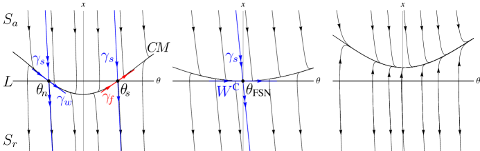
Figure 5: Reduced flow (11) of the fvdP equation (1) shown in a neighbourhood of the upper fold curve $L$ (defined by $x=1,y=-\frac{2}{3}$) for $\overline{\omega}=1,b=0.01$, and (a) $a=1+\frac{b}{2}$, (b) $a=1+b$ and (c) $a=1+\frac{3b}{2}$. In panel (a) where $a<1+b$, there is a folded node ($\theta_{n}$) and a folded saddle ($\theta_{s}$). The strong and weak eigendirections of the folded node are denoted by $\gamma_{s}$ and $\gamma_{w}$, respectively. Similarly, the singular canard and faux canard of the folded saddle are labelled $\gamma_{s}$ and $\gamma_{f}$, respectively. Note that there is a heteroclinic connection $CM$ from $\theta_{n}$ to $\theta_{s}$. In particular, $\gamma_{w}$ is tangent to $CM$ at $\theta_{n}$, and $\gamma_{f}$ is tangent to $CM$ at $\theta_{s}$. In panel (b) where $a=1+b$, the folded singularities merge to a FSN I (indicated by $\theta_{\text{FSN}}$). In this case, the singular strong canard of the folded node merges with the maximal canard of the folded saddle. Meanwhile, the singular weak canard of the folded node merges with the faux canard of the folded saddle to become the center manifold $W^{C}$ of the FSN I. In panel (c) where $a>1+b$, the folded singularities (and associated singular canards) have been destroyed in the FSN I bifurcation, and there are no canard dynamics.

In the FSN limit, the standard folded node/folded saddle theory requires modification. For the FSN I, the following results have recently been proved in [54], valid for $0<\operatorname{\varepsilon}\ll 1$ and $\mu=\mathcal{O}(\operatorname{\varepsilon}^{\alpha})$ where $\alpha\geq 1/4$:

1. The singular strong canard of the folded node perturbs to the primary maximal strong canard. The singular canard of the folded saddle perturbs to a maximal canard.

2. There exists a heteroclinic connection $CM$ between the folded nodes and folded saddles of (12). This heteroclinic perturbs to a canard-faux canard solution $CM^{\operatorname{\varepsilon}}$ that corresponds to both the primary weak canard of the folded node and the faux canard of the folded saddle (faux canards are the equivalent of singular faux canards for $0<\varepsilon\ll 1$).

3. There exist $\mathcal{O}(\operatorname{\varepsilon}^{-1/4})$ canards and faux canards.

Thus, canards and faux canards of the FSN I oscillate about an axis of rotation, which is approximately given by the heteroclinic $CM$ that connects the folded node and folded saddle (see Figure 5(a) for instance). For the fvdP, we find that $CM:=\left\{(x,y,\theta)\in S:x=a+b\cos\theta\right\}.$ We study the associated maximal canards of (1) in Section 3.

Remark 1.

For the forced vdP equation (1), FSN II points are codimension-2 bifurcation points of the desingularised flow (corresponding to $\overline{\omega}=0$), and constitute a special case of the FSN I. They can be analyzed using the approach presented in [37].

3 Loci of the Maximal Canards for Low Forcing Frequencies

In this section, we analyse system (1) with low-frequency forcing ($\omega=\operatorname{\varepsilon}\overline{\omega}$). We prove Theorem 1.1, demonstrating that, for $b=\mathcal{O}(\sqrt{\operatorname{\varepsilon}})$, formula (2) gives the branches of the folds of the primary maximal canards and that for each value of $a$ in between the fold curves, there are two primary maximal canards of system (1) given in parameter space by (7). More precisely, we analyze the FSN I points to show that formula (2) gives the locus of points at which the primary strong canard of a folded node point merges with the folded saddle maximal canard. We present the analysis for the FSN I that occurs for $a=1-b$ and note that the FSN I at $a=1+b$ is treated similarly.

For the analysis with low-frequency forcing, we first translate the FSN I at $a=1-b$ to the origin

$$u=x-1,\quad v=y+\frac{2}{3},\quad\eta=a-1+b,$$

so that (1) is transformed to

$$\begin{split}u^{\prime}&=v-\left(u^{2}+\frac{1}{3}u^{3}\right),\\ v^{\prime}&=\operatorname{\varepsilon}\left(-u+\eta+b(\cos\theta-1)\right),\\ \theta^{\prime}&=\operatorname{\varepsilon}\overline{\omega}.\end{split}$$ (13)

We then inflate the FSN I singularity to a hypersphere using the spherical blow-up transformation:

$$u=\overline{r}^{2}\overline{u},\quad v=\overline{r}^{4}\overline{v},\quad\theta=\overline{r}\overline{\theta},\quad\operatorname{\varepsilon}=\overline{r}^{4}\overline{\operatorname{\varepsilon}}.$$

Moreover, we rescale the parameters $b$ and $\eta$ as

$$b=\sqrt{\operatorname{\varepsilon}}\beta,\quad\eta=\operatorname{\varepsilon}\gamma,$$

where $\beta=\mathcal{O}(1)$ and $\gamma=\mathcal{O}(1)$. Also, we append the trivial equation $\operatorname{\varepsilon}^{\prime}=0$ to system (13) and take $\mu>0$ sufficiently small. The (spherical) blow-up transformation is a map from $B:=S^{3}\times[-\mu,\mu]$ into $\mathbb{R}^{4}$. We examine the vector fields induced by this coordinate transformation in two useful coordinate charts: the entry-exit chart (or phase-directional chart) $K_{1}:\{\overline{v}=1\}$ and the rescaling (or central) chart $K_{2}:\{\overline{\operatorname{\varepsilon}}=1\}$, beginning with $K_{1}$.

In chart $K_{1}$, the blow-up coordinates are

$$u=r_{1}^{2}u_{1},\quad v=r_{1}^{4},\quad\theta=r_{1}\theta_{1},\quad\operatorname{\varepsilon}=r_{1}^{4}\operatorname{\varepsilon}_{1},$$ (14)

where the subscript corresponds to the chart number. The governing equations are

$$\begin{split}\dot{u}_{1}&=1-u_{1}^{2}-\frac{1}{3}r_{1}^{2}u_{1}^{3}-\frac{1}{2}\operatorname{\varepsilon}_{1}u_{1}F,\\ \dot{r}_{1}&=\frac{1}{4}r_{1}\operatorname{\varepsilon}_{1}F,\\ \dot{\theta}_{1}&=r_{1}\operatorname{\varepsilon}_{1}\overline{\omega}-\frac{1}{4}\operatorname{\varepsilon}_{1}\theta_{1}F,\\ \dot{\operatorname{\varepsilon}}_{1}&=-\operatorname{\varepsilon}_{1}^{2}F,\end{split}$$ (15)

where $F(u_{1},\theta_{1},r_{1})=-u_{1}+r_{1}^{2}\operatorname{\varepsilon}_{1}\gamma+\beta\sqrt{\operatorname{\varepsilon}_{1}}\left(\cos(r_{1}\theta_{1})-1\right)$, and we have desingularised the vector field by a factor of $r_{1}^{2}$ and recycled the overdot to denote the derivative with respect to the new time. The hyperplanes $\{r_{1}=0\}$ and $\{\operatorname{\varepsilon}_{1}=0\}$ are invariant. In the invariant subspace $\{r_{1}=0\}$, $\theta_{1}=0$ is an attracting fixed point. The line

$$\ell_{u}=\{(u_{1},r_{1},\theta_{1},\operatorname{\varepsilon}_{1})=(u_{1},0,0,0)\}$$

is invariant, and on it the system dynamics are governed by $\dot{u}_{1}=1-u_{1}^{2}$. Furthermore, on $\ell_{u}$ there are attracting and repelling fixed points $p_{a}=(1,0,0,0)$ and $p_{r}=(-1,0,0,0)$, which, respectively, have center manifolds $N_{a,1}$ and $N_{r,1}$ in the half space $\operatorname{\varepsilon}_{1}>0$.

In order to demonstrate the existence of the primary maximal canards, we will show that there is a heteroclinic connection between $p_{a}$ and $p_{r}$ in the hyperplane $\{r_{1}=0\}$ and that this heteroclinic orbit persists for sufficiently small values of $r_{1}$, using Melnikov theory. The persistent connections correspond to the primary maximal canards. We carry out the relevant analysis in the rescaling chart $K_{2}$, where the blow-up transformation is given by

$$u=r_{2}^{2}u_{2},\quad v=r_{2}^{4}v_{2},\quad\theta=r_{2}\theta_{2},\quad\operatorname{\varepsilon}=r_{2}^{4}.$$ (16)

Note that $r_{2}=\operatorname{\varepsilon}^{1/4}$, so that chart $K_{2}$ corresponds to an $\operatorname{\varepsilon}$-dependent rescaling of the forced vdP equation. Also, the coordinates in the two charts are related via the following transformation:

$$r_{2}=r_{1}\operatorname{\varepsilon}_{1}^{1/4},\quad u_{2}=u_{1}\operatorname{\varepsilon}_{1}^{-1/2},\quad v_{2}=\operatorname{\varepsilon}_{1}^{-1},\quad\theta_{2}=\theta_{1}\operatorname{\varepsilon}_{1}^{-1/4},$$

where $\operatorname{\varepsilon}_{1}>0$.

In chart $K_{2}$, the blown-up system (13) is

$$\begin{split}\dot{u}_{2}&=v_{2}-u_{2}^{2}-\frac{1}{3}r_{2}^{2}u_{2}^{3},\\ \dot{v}_{2}&=-u_{2}+r_{2}^{2}\gamma+\beta\left(\cos(r_{2}\theta_{2})-1\right),\\ \dot{\theta}_{2}&=r_{2}\,\overline{\omega},\end{split}$$ (17)

where we have desingularised the vector field (i.e., rescaled by $r_{2}^{2}$) and again recycled the overdot, this time to denote the derivative with respect to the new time $t_{2}$. This system is singularly perturbed with fast variables $(u_{2},v_{2})$ and slow variable $\theta_{2}$. Rewriting the blown-up system in non-autonomous form, we have

$$\begin{split}{\dot{u}}_{2}&=v_{2}-u_{2}^{2}-\frac{1}{3}r_{2}^{2}u_{2}^{3},\\ {\dot{v}}_{2}&=-u_{2}+r_{2}^{2}\gamma+\beta\left(\cos(r_{2}^{2}\overline{\omega}t_{2})\cos(r_{2}\theta_{2,0})-1\right)-\beta\sin(r_{2}^{2}\overline{\omega}t_{2})\sin(r_{2}\theta_{2,0}),\end{split}$$ (18)

where $\theta_{2,0}$ is an arbitrary phase. This is the system we will analyse in chart $K_{2}$. For $\overline{\omega}$ and $t_{2}$ of ${\cal O}(1)$, we have

$$\cos(r_{2}^{2}\overline{\omega}t_{2})\cos(r_{2}\theta_{2,0})-1 =\mathcal{O}(r_{2}^{2})\text{ as }r_{2}\to 0,$$

$$\sin(r_{2}^{2}\overline{\omega}t_{2})\sin(r_{2}\theta_{2,0}) =\mathcal{O}(r_{2}^{3})\text{ as }r_{2}\to 0.$$

The unperturbed problem corresponding to (18) is obtained by setting $r_{2}=0$,

$$\begin{split}u^{\prime}_{2}&=v_{2}-u_{2}^{2},\\ v^{\prime}_{2}&=-u_{2}.\end{split}$$ (19)

This system is Hamiltonian with Hamiltonian function

$$H(u_{2},v_{2})=e^{-2v_{2}}\left(u_{2}^{2}-v_{2}-\frac{1}{2}\right),$$

and non-canonical formulation

$$\dot{u}_{2} =\frac{1}{2}e^{2v_{2}}\frac{\partial H}{\partial v_{2}},$$

$$\dot{v}_{2} =-\frac{1}{2}e^{2v_{2}}\frac{\partial H}{\partial u_{2}}.$$

The level curves of $H$ are presented in Figure 6.

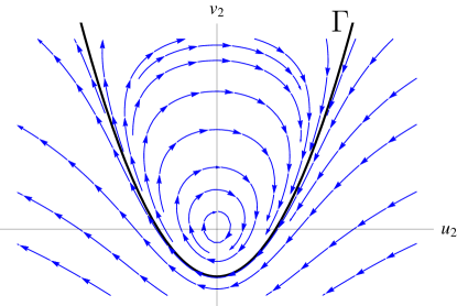
Figure 6: Contours of the Hamiltonian function $H$. Periodic solutions of (19) correspond to level sets with $-\frac{1}{2}\leq H<0$. Unbounded solutions of (19) correspond to $H>0$. The $H=0$ contour, $\Gamma$, is the heteroclinic connecting the points $p_{a}$ and $p_{r}$ at infinity.

The contour $\Gamma$ separates closed trajectories from unbounded orbits and has the explicit time parametrization

$$(u_{2,\Gamma},v_{2,\Gamma})=\left(-\frac{1}{2}t_{2},\frac{1}{4}t_{2}^{2}-\frac{1}{2}\right).$$

The separatrix $\Gamma$ corresponds to the singular strong canard of the FSN I. In geometric terms, it is a heteroclinic orbit that lies on the upper-hemisphere and connects the fixed points $p_{a}$ and $p_{r}$, which both lie on the equator of the blown-up sphere.

We now use the Melnikov method to analyse the persistence of $\Gamma$ under small-amplitude perturbations. As applied to (18), Melnikov theory measures the splitting distance $D$ between the curves of solutions of the perturbed system that are forward and backward asymptotic to $p_{r}$ and $p_{a}$, respectively. We develop $D$ in an asymptotic series in the small parameter $r_{2}$:

$$D(r_{2})=d_{1}r_{2}^{2}+d_{2}r_{2}^{3}+\cdots,$$

where the terms in the Melnikov integral are given by

$$d_{1} =\int_{-\infty}^{\infty}\nabla\left.H\right|_{\Gamma}\boldsymbol{\cdot}\begin{pmatrix}-\frac{1}{3}u_{2,\Gamma}^{3}\\ \gamma+\frac{\beta}{r_{2}^{2}}\left(\cos(r_{2}^{2}\overline{\omega}t_{2})\cos(r_{2}\theta_{2,0})-1\right)\end{pmatrix}\,dt_{2},$$

$$d_{2} =\int_{-\infty}^{\infty}\nabla\left.H\right|_{\Gamma}\boldsymbol{\cdot}\begin{pmatrix}0\\ -\frac{\beta}{r_{2}^{3}}\sin(r_{2}^{2}\overline{\omega}t_{2})\sin(r_{2}\theta_{2,0})\end{pmatrix}\,dt_{2}.$$

We note that the integrand in $d_{2}$ is an odd function of $t_{2}$ so the integral evaluates to zero and the sine term has no contribution to the distance measurement $D$. We also note that the $\frac{\cos(r_{2}^{2}\overline{\omega}t_{2})\cos(r_{2}\theta_{2,0})-1}{r_{2}^{2}}$ term in $d_{1}$ is $\mathcal{O}(1)$ with respect to $r_{2}$. The integral $d_{1}$ was evaluated by taking $\cos z=\operatorname{Re}(e^{iz})$, completing the square in the exponential, and deforming the contour in the complex plane. The result is

$$d_{1}=\frac{e\sqrt{2\pi}}{r_{2}^{2}}\left\{\beta-r_{2}^{2}\left(\frac{1}{8}+\gamma\right)-\beta e^{-\frac{1}{2}r_{2}^{4}\overline{\omega}^{2}}\cos(r_{2}\theta_{2,0})\right\}.$$

Substituting this into the bifurcation equation $D=0$, we have

$$r_{2}^{2}\left(\frac{1}{8}+\gamma\right)+\beta\cos(r_{2}\theta_{2,0})\left(e^{-\frac{1}{2}r_{2}^{4}\overline{\omega}^{2}}-1\right)=0.$$

Thus, reverting to the parameters $a,b,\operatorname{\varepsilon}$, and $\overline{\omega}$, we see that the primary maximal canards for the FSN I are given by

$$a=1-\frac{\operatorname{\varepsilon}}{8}-b\cos(\theta_{0})\exp\left(-\frac{\operatorname{\varepsilon}\overline{\omega}^{2}}{2}\right),$$ (20)

which is (7). We remark that $\theta_{0}$ is the arbitrary phase $\theta_{2,0}$ in the original $\theta$ coordinate (i.e., $\theta_{0}=r_{2}\theta_{2,0}$). This completes the demonstration that (7) holds for low-frequency forcing, giving the locus of points at which the primary maximal canards exist. Moreover, one also sees that, for each $\overline{\omega}$, the folds of the primary maximal canards at the endpoints of these parameter intervals are given by

$$a=1-\frac{\operatorname{\varepsilon}}{8}\pm b\exp\left(-\frac{\operatorname{\varepsilon}\overline{\omega}^{2}}{2}\right),$$ (21)

which is precisely (2). The loci in the $(\overline{\omega},a)$ plane of the folds of maximal canards mark the upper and lower boundaries of the regime in which the primary maximal canards exist. This completes the proof of Theorem 1.1.

Remark 2.

For $\omega=\operatorname{\varepsilon}\overline{\omega}$, one may extend the result of Theorem 1.1 to the parameter regime in which $b=\mathcal{O}(\operatorname{\varepsilon}^{\frac{1}{4}})$. Let $b=\operatorname{\varepsilon}^{\frac{1}{4}}\beta$ and $\eta=\operatorname{\varepsilon}^{\frac{3}{4}}\gamma$, where $\beta$ and $\gamma$ are ${\cal O}(1)$ with respect to $\operatorname{\varepsilon}$. Then, the perturbation terms in the $v_{2}$ component of the non-autonomous system become:

$$r_{2}\left[\gamma+\frac{\beta}{r_{2}^{2}}\left(\cos(r_{2}^{2}\overline{\omega}t_{2})\cos(r_{2}\theta_{2,0})-1\right)-\frac{\beta}{r_{2}^{2}}\sin(r_{2}^{2}\overline{\omega}t_{2})\sin(r_{2}\theta_{2,0})\right].$$

Here, the even terms are ${\cal O}(r_{2})$ as $r_{2}\to 0$, so that one may proceed with a similar Melnikov calulation as above, and the odd terms again do not contribute to leading order in the Melnikov calculation.

We further note that a blow-up and Melnikov computation similar to that just presented for the FSN I points may be done for the folded nodes and folded saddles, and this gives the location of the maximal canards as

$$\theta_{n,s}(k)\approx 2k\pi\pm\cos^{-1}\left(\frac{1-a-\operatorname{\varepsilon}/8}{b}+\mathcal{O}(b)\right),\qquad k\in\mathbb{Z}.$$

See also equation (42) in [2].

4 Loci of the Torus Canards and Their Folds for Intermediate- and High-Frequency Forcing

In this section, we study system (1) in the intermediate-frequency regime with $\omega=\sqrt{\operatorname{\varepsilon}}\Omega$ and $\Omega={\cal O}(1)$, as well as in the high-frequency regime with $\omega={\cal O}(1)$. We prove Theorem 1.2, demonstrating that system (1) possesses a family of torus canards in the intermediate-frequency regime, in between the two fold curves (3) of these torus canards. The central methods used in the proof are geometric desingularization –in which we use a cylindrical blow-up of the fold curve rather than a spherical blow-up as used in the previous section– and a Melnikov calculation to identify the parameter values for which the torus canards exist. After Theorem 1.2 is established, we also prove Corollary 1.3 for the high-frequency regime.

In the intermediate-frequency regime, system (1) is equivalent to

$$\begin{split}x^{\prime}&=y-f(x),\\ y^{\prime}&=\operatorname{\varepsilon}(-x+a+b\cos\theta),\\ \theta^{\prime}&=\sqrt{\operatorname{\varepsilon}}\Omega.\end{split}$$ (22)

First, we rectify the fold curve so that it coincides with the $\theta$ axis,

$$u=x-1,\quad v=y+\frac{2}{3},\quad\alpha=a-1.$$

Also, we recall

$$\alpha=\operatorname{\varepsilon}\tilde{\alpha},\quad b=\operatorname{\varepsilon}\tilde{\beta},$$

where $\tilde{\alpha}$ and $\tilde{\beta}$ are ${\cal O}(1)$ with respect to $\operatorname{\varepsilon}$. This transforms (22) to the following system:

$$\begin{split}u^{\prime}&=v-u^{2}-\frac{1}{3}u^{3},\\ v^{\prime}&=-\operatorname{\varepsilon}u+\operatorname{\varepsilon}^{2}(\tilde{\alpha}+\tilde{\beta}\cos\theta),\\ \theta^{\prime}&=\sqrt{\operatorname{\varepsilon}}\Omega.\end{split}$$ (23)

Next, we perform the following cylindrical blow-up transformation:

$$u=\overline{r}\overline{u},\quad v=\overline{r}^{2}\overline{v},\quad\operatorname{\varepsilon}=\overline{r}^{2}\overline{\operatorname{\varepsilon}},$$ (24)

which transforms the circle of fold points into a torus. (This contrasts with the spherical blow-up of the FSN I point in the previous section.) Append the trivial equation $\operatorname{\varepsilon}^{\prime}=0$ to system (23) and let $\mu>0$ be sufficiently small. For each $\theta\in\mathbb{S}^{1}$ and for all non-negative values of the system parameters, the coordinate change is a map from $B:=\mathbb{S}^{2}\times[-\mu,\mu]$ into $\mathbb{R}^{3}$. We examine the vector fields induced by (23) in two useful coordinate charts: the entry-exit chart (or phase-directional chart) $K_{1}=\{\overline{v}=1\}$ and the rescaling chart $K_{2}=\{\overline{\operatorname{\varepsilon}}=1\}$.

In chart $K_{1}$, the coordinates are

$$u=r_{1}u_{1},\quad v=r_{1}^{2},\quad\operatorname{\varepsilon}=r_{1}^{2}\operatorname{\varepsilon}_{1}.$$

Setting $F(u_{1},r_{1},\operatorname{\varepsilon}_{1},\theta,\tilde{\alpha},\tilde{\beta})=-u_{1}+\operatorname{\varepsilon}_{1}r_{1}(\tilde{\alpha}+\tilde{\beta}\cos(\theta))$, we find that the system in chart $K_{1}$ is

$$\begin{split}\dot{u}_{1}&=1-u_{1}^{2}-\frac{1}{3}r_{1}u_{1}^{3}-\frac{u_{1}\operatorname{\varepsilon}_{1}}{2}F,\\ \dot{r}_{1}&=\frac{r_{1}\operatorname{\varepsilon}_{1}}{2}F,\\ \dot{\theta}&=\sqrt{\operatorname{\varepsilon}_{1}}\Omega,\\ \dot{\operatorname{\varepsilon}}_{1}&=-\operatorname{\varepsilon}_{1}^{2}F,\end{split}$$ (25)

where we have desingularised the vector field by rescaling the time variable by a factor of $r_{1}$ and recycled the overdot. In the phase space of (25), the hyperplanes $\{r_{1}=0\}$ and $\{\operatorname{\varepsilon}_{1}=0\}$ are invariant. In addition, for every $(\tilde{\alpha},\tilde{\beta})$, there is an invariant line

$$\ell_{u}=\{(u_{1},r_{1},\operatorname{\varepsilon}_{1})=(u_{1},0,0)\}$$

on which the dynamics are governed by $\dot{u}_{1}=1-u_{1}^{2}$ and $\dot{\theta}=0$. Moreover, for every $(\tilde{\alpha},\tilde{\beta})$, the points

$$p_{a}=(1,0,0)\quad{\rm and}\quad p_{r}=(-1,0,0)$$

are attracting and repelling fixed points, respectively, on $\ell_{u}$, and they have two-dimensional center manifolds $N_{a,1}$ and $N_{r,1}$ in the half-space $\operatorname{\varepsilon}_{1}>0$.

In order to establish the existence of the torus canards, we now hook up the dynamics observed in chart $K_{1}$ to those in chart $K_{2}$. In chart $K_{2}$, the coordinates are

$$u=r_{2}u_{2},\quad v=r_{2}^{2}v_{2},\quad\operatorname{\varepsilon}=r_{2}^{2},$$ (26)

and these coordinates are related to those of chart $K_{1}$ via the following coordinate transformation:

$$u_{2}=u_{1}\operatorname{\varepsilon}_{1}^{-1/2},\quad v_{2}=\operatorname{\varepsilon}_{1}^{-1},\quad r_{2}=r_{1}\operatorname{\varepsilon}_{1}^{1/2},$$

where $\operatorname{\varepsilon}_{1}>0$.

In chart $K_{2}$, the system is

$$\dot{u}_{2} =v_{2}-u_{2}^{2}-\frac{1}{3}r_{2}u_{2}^{3},$$

$$\dot{v}_{2} =-u_{2}+r_{2}\left(\tilde{\alpha}+\tilde{\beta}\cos(\Omega t_{2}+\theta_{0})\right),$$ (27)

where we have also rescaled time by a factor of $r_{2}$ in order to desingularise the vector field (with $t_{2}$ denoting this rescaled time variable), recycled the overdot again now to denote the derivative with respect to $t_{2}$, and written the system as a non-autonomous system. For reference, we emphasize the relation $\sqrt{\operatorname{\varepsilon}}=r_{2}$. We now show that system (4) possesses a special family of homoclinic orbits, connecting the point at infinity to itself, which implies that the orbits connect the points $p_{r}$ and $p_{a}$ identified in chart $K_{1}$. These orbits correspond to singular torus canards of the original system (22).

The unperturbed problem associated to system (4) is given by

$$\dot{u}_{2} =v_{2}-u_{2}^{2},$$

$$\dot{v}_{2} =-u_{2},$$

which is the same as (19). As shown in the previous section, this unperturbed system is Hamiltonian

$$H(u_{2},v_{2})=e^{-2v_{2}}\left(u_{2}^{2}-v_{2}-\frac{1}{2}\right).$$

Along the level set $\Gamma:=\{H=0\}$, which is the separatrix between bounded and unbounded solutions (see Figure 6), the solutions are given explicitly by

$$u_{2,\Gamma}(t_{2})=-\frac{t_{2}}{2},\qquad v_{2,\Gamma}(t_{2})=\frac{t_{2}^{2}}{4}-\frac{1}{2}.$$

In the language of dynamical systems, it is a homoclinic orbit to infinity.

With the above information about the unperturbed system in hand, we now turn to show that $\Gamma$ persists for sufficiently small values of $r_{2}$ in (4). We use a straightforward generalization of Proposition 3.5 of [36], where we note that the perturbation terms there are strictly autonomous, whereas here the perturbation terms also include a small-amplitude, time-periodic function, and a compactification of the phase space can be used. Moreover, we observe that the parameter there, $\lambda_{2}$, is also treated as being a small variable via the linear scaling of $\lambda$ with $r_{2}$, whereas here we have chosen instead to scale the parameters $\alpha$ and $b$ with $\operatorname{\varepsilon}$ from the outset and to treat $\tilde{\alpha},\tilde{\beta}={\cal O}(1)$ as parameters. In this manner, $r_{2}$ is the only small variable in the analysis here.

The splitting distance between the manifolds $N_{a,2}$ and $N_{r,2}$ for system (4) is

$$D(r_{2})=d_{r_{2}}r_{2}+\cdots.$$

Here, the dependence of the Melnikov function on the system parameters is implicit. We find

$$d_{r_{2}} =\int_{-\infty}^{\infty}\nabla\left.H\right|_{\Gamma}\boldsymbol{\cdot}\begin{pmatrix}-\frac{1}{3}u_{2,\Gamma}^{3}\\ \tilde{\alpha}+\tilde{\beta}\cos(\Omega t_{2}+\theta_{0})\end{pmatrix}\,dt_{2}$$

$$=-\frac{e}{2}\sqrt{2\pi}\left(\frac{1}{8}+\tilde{\alpha}+\tilde{\beta}e^{-\frac{\Omega^{2}}{2}}\cos(\theta_{0})\right),$$ (28)

where the last term in the integral was evaluated by using $\cos(z)={\rm Re}(e^{iz})$, completing the square on the exponential, and shifting the contour in the complex plane. Hence, reverting to the given parameters, we see that to leading order the splitting distance is

$$D=-\frac{e}{2}\sqrt{2\pi}\left[\frac{\sqrt{\operatorname{\varepsilon}}}{8}+\frac{a-1}{\sqrt{\operatorname{\varepsilon}}}+\frac{b}{\sqrt{\operatorname{\varepsilon}}}e^{-\frac{\Omega^{2}}{2}}\cos(\theta_{0})\right].$$ (29)

Therefore, for each $b$ satisfying the hypotheses of the theorem and for $\operatorname{\varepsilon}$ small enough, the simple zeroes of the Melnikov function are given in the $(a,\Omega)$ plane by

$$a=1-\frac{\operatorname{\varepsilon}}{8}-be^{-\frac{\Omega^{2}}{2}}\cos(\theta_{0}).$$ (30)

This formula, which is exactly (7) in the intermediate-frequency regime, gives the parameter values for which system (4) has a one-parameter ($\theta_{0}$) family of persistent homoclinic orbits, and these persistent homoclinic orbits of (4) are the torus canards of (22).

Also, as a direct corollary, we observe that the envelope of the family of torus canards is given by

$$a=1-\frac{\operatorname{\varepsilon}}{8}\pm b\exp\left(-\frac{\Omega^{2}}{2}\right),$$ (31)

which is precisely formula (3). This completes the proof of Theorem 1.2.

To conclude this section, we prove Corollary 1.3. The proof follows by extending, in a straight forward manner, the above analysis of the persistent homoclinics and the folds of the torus canards in the proof of Theorem 1.2 for the intermediate-frequency forcing regime to the high-frequency forcing regime. In particular, in the high-frequency regime, $\omega={\cal O}(1)$, which corresponds to taking $\Omega={\cal O}(1/\sqrt{\operatorname{\varepsilon}})$ in the above analysis. Following exactly along the above calculations, we see that the geometric desingularization method yields the same equations (4) in chart $K_{2}$, but now the small-amplitude time-periodic forcing term has high-frequency $\Omega={\cal O}(1/\sqrt{\operatorname{\varepsilon}})$. Hence, the suitable version of the Melnikov theory is that for rapidly forced systems, and the splitting distance along $\Gamma$ is again given by (31), which is now exponentially small in $\operatorname{\varepsilon}$, since $\Omega={\cal O}(1/\sqrt{\operatorname{\varepsilon}})$. See for example [12]. This completes the proof of Corollary 1.3.

The result of this Corollary for the high-frequency regime also agrees well with the results obtained from numerical simulations. In Figure 7, for $\omega=O(1)$, we present a computation of the distance between the two folds of maximal primary canards as a function of $\operatorname{\varepsilon}$. We gathered the control points obtained for various computations for eleven fixed values of $\operatorname{\varepsilon}$, decreasing from $3\cdot 10^{-3}$ down to $8\cdot 10^{-4}$ and plotted them on a logarithmic scale. The hyperbolic shape of the resulting curve confrms that this distance is exponentially small in $\operatorname{\varepsilon}$ as $\operatorname{\varepsilon}$ tends to $0$.

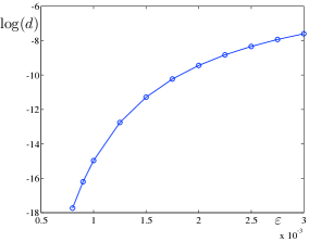
Figure 7: Width of the canard region in the $\omega=O(1)$ regime, as a function of $\operatorname{\varepsilon}$ for $b=0.01$.

5 Secondary Canards

Having established the existence of the primary strong canards and their folds, we now turn our attention to the secondary canards of the folded nodes of (1), which exist in the low-frequency forcing regime $\omega=\operatorname{\varepsilon}\overline{\omega}$. By definition, secondary canards lie in the transverse intersections of the invariant slow manifolds $S_{a}^{\operatorname{\varepsilon}}$ and $S_{r}^{\operatorname{\varepsilon}}$. A representative example of these manifolds and their intersections (i.e. the secondary canards) is shown in Figure 8. These manifolds are computed from curves of initial conditions traced on the attracting and repelling sheets, respectively, of the critical manifold $S$, up to a cross-section at fixed angle $\theta$ corresponding to the maximal torus canard [13, 14]:

$$\Sigma_{n}=\left\{\theta_{n}=\cos^{-1}\left(\frac{1-a-\operatorname{\varepsilon}/8}{b}+\mathcal{O}(b)\right)\right\}.$$

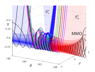
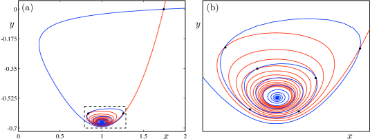
Figure 8: Attracting (red) and repelling (blue) slow manifolds of system (1) for $a=0.9935,b=0.01,\omega=0.005$, and $\operatorname{\varepsilon}=0.05$, together with a stable MMO with 1 LAO and 6 SAOs found for the same parameter values by direct simulation. Bottom row: invariant slow manifolds $S_{a}^{\operatorname{\varepsilon}}$ (red) and $S_{r}^{\operatorname{\varepsilon}}$ (blue) of system (1) in the cross-section $\Sigma_{n}$. The secondary canards are identified as the intersections (black dots) of $S_{a}^{\operatorname{\varepsilon}}$ and $S_{r}^{\operatorname{\varepsilon}}$.

In Section 5.1, we study the folds of the secondary canards and investigate how they change in the $(\omega,a)$ plane under variation of the forcing amplitude $b$ (analogous to the folds of the primary canards). We then investigate in Section 5.2 how large-amplitude oscillations can grow from small-amplitude oscillations.

5.1 Continuation of Secondary Canards

As shown in Figure 8, the invariant slow manifolds $S_{a}^{\operatorname{\varepsilon}}\cap\Sigma_{n}$ and $S_{r}^{\operatorname{\varepsilon}}\cap\Sigma_{n}$ spiral around one another, which is typical of a folded node. More precisely, let $\mu:=\lambda_{w}/\lambda_{s}$, $|\lambda_{w}|<|\lambda_{s}|$, denote the eigenvalue ratio of a folded node, regarded as an equilibrium of the desingularised system (12). Provided $\operatorname{\varepsilon}$ is sufficiently small and $\mu$ is bounded away from zero, the total number of (primary and secondary) maximal canards is $s_{\max}+1$, where

$$s_{\max}=\lfloor\frac{\mu+1}{2\mu}\rfloor,$$

and $\lfloor\cdot\rfloor$ denotes the floor function. In particular, a persistent branch of secondary canards bifurcates from the weak canard in a transcritical bifurcation for odd integer values of $\mu^{-1}$ [55].

Remark 3.

The $k^{\text{th}}$ secondary canard exhibits $k$ small oscillations about the weak canard for $k=1,2,\ldots,s_{\max}-1$. These small oscillations are localized to an $\mathcal{O}(\sqrt{\operatorname{\varepsilon}})$ neighbourhood of the folded node [55, 56]. Moreover, trajectories on $S_{a}^{\operatorname{\varepsilon}}$ situated between $\gamma_{k-1}$ and $\gamma_{k}$, $k=1,2,\ldots,s_{\max}$ execute $k$ small oscillations about the weak canard, where $\gamma_{0}$ and $\gamma_{s_{\max}}$ correspond to the primary strong canard and primary weak canard, respectively.

By tracking the resonances $\mu^{-1}=2k+1,k=0,1,2,\ldots$, we can follow (in the singular limit) the locations in the $(\overline{\omega},a)$ plane where the secondary canards are born. Figure 9 shows an example for $b=1$. The non-singular $(\omega,a)$ plane shows that only the folds of canards corresponding to the FSN I and the degenerate folded node extend into the intermeditate frequency regime. All other branches of folds of canards are restricted to the low-frequency regime $\omega=\mathcal{O}(\operatorname{\varepsilon})$.

Remark 4.

Note that the resonance curves in Figure 9 bear no resemblance to the curves of folds of secondary canards in Figure 3. This is to be expected since $b=\mathcal{O}(\sqrt{\operatorname{\varepsilon}})$ in Figure 3, which implies that $\mu=\mathcal{O}(\sqrt{\operatorname{\varepsilon}})$ and the folded node theory does not apply.

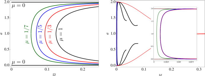
Figure 9: Resonance curves for $b=1$, and (a) $\operatorname{\varepsilon}=0$ and (b) $\operatorname{\varepsilon}=0.01$. In (b), the theoretically computed curve of maximal canards for the FSN I (2) are shown in red. Inside this envelope, there are two black resonance curves. Both correspond to the numerical continuation of folds of maximal canards. The outermost black curve corresponds to the FSN I (i.e. where $\mu=0$). Note that (2) breaks down when $\omega$ is no longer $\mathcal{O}(\operatorname{\varepsilon})$. The inner black curve corresponds to the maximal canard of the degenerate folded node (i.e. where $\mu=1$). The inset shows the numerical continuation of the folds of canards corresponding to $\mu=1$ and $\mu=1/3$. In particular, for the $\mu=1$ resonance, we compare the numerically computed result (blue) and the theoretical result obtained in (32) (red), and find that there is excellent agreement away from the FSN I boundaries.

For the degenerate node ($\mu=1$), a Melnikov computation similar to that in Sections 3 and 4 shows that the locus of the primary maximal canard of the degenerate folded node in the $(\overline{\omega},a)$ plane is

$$a=1-\frac{\operatorname{\varepsilon}}{8}\pm\sqrt{b^{2}-\frac{1}{64\overline{\omega}^{2}}}\exp\left(-\frac{1}{2}\operatorname{\varepsilon}\overline{\omega}^{2}\right),$$ (32)

which holds provided $\overline{\omega}=\mathcal{O}(1),\sqrt{b^{2}-\frac{1}{64\overline{\omega}^{2}}}=\mathcal{O}(\operatorname{\varepsilon})$ and $\sqrt{b^{2}-(1-a)^{2}}=\mathcal{O}(\sqrt{\operatorname{\varepsilon}})$. The inset of Figure 9 shows that there is excellent agreement between this theoretically computed curve and the curve obtained from numerical continuation. The deviation between theoretical and numerical results for this degenerate folded node maximal canard starts to become significant when the degenerate node branches approach the FSN I branches. We note an important implication: all secondary canards due to folded nodes are restricted to the region of the $(\omega,a)$ plane bounded by $\omega=0$, the locus of the folds of maximal canards of the FSN I and the locus of the maximal canards of the degenerate folded node.

As was the case for the numerical continuation of the folds of the primary canards and the folds of the torus canards, the numerical continuation of the maximal secondary canards is done by solving families of boundary-value problems and computing branches of such solutions using pseudo-arclength continuation. Along these branches, a number of fold points can be detected, and then the curves of folds of secondary canards can be continued in two parameters. For a representative set of parameter values, the folds of the first, second, $\ldots$, tenth secondary canards (i.e., with respectively one, two, $\ldots$, ten loops) are shown in the $(\omega,a)$ plane in Figure 3. The outermost envelope in Figure 3 are the curves of folds of primary canards. The rightmost path enclosed by the fold curve of the primary strong canards represents the fold curve of the first (1-loop) secondary canard, and each successive curve to the left represents a family of folds of secondary canards with one additional loop. These branches of folds of secondary canards emanate from the FSN I points at $a=1-\frac{\operatorname{\varepsilon}}{8}\pm b$. As $\omega$ is increased, the corresponding pairs of $n$-loop branches come together at turning points.

It is also useful to examine projections of the secondary canards onto the $(x,y)$ plane. In Figure 10, we show the first three maximal secondary canards, with respectively, one loop (yellow), two loops (red), and three loops (blue). The highest loops of the 2-loop and 3-loop maximal secondary canards are observed to lie extremely close to the single loop of the 1-loop maximal secondary canard. The same holds for all of the higher-loop secondary canards, as well. Also, the second loop of the 2-loop canard lies inside the first loop, and it lies extremely close to the second loop of the 3-loop canard. In addition, for even smaller values of the forcing frequency $\omega$, the $y$-intercepts of the return jumps increase. Moreover, these $y$-intercepts diverge to $\infty$ in the limit $\omega\to 0$. In fact, in this limit, the maximal secondary canards collapse onto the primary strong canard, consistent with the observation that the branches of maximal secondary canards emanate from the same FSN I points as the primary canards do.

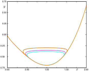
Figure 10: Projection of the 1-loop (yellow), 2-loop (red), and 3-loop (blue) secondary canards of (1) shown for $\omega=0.01$, $\operatorname{\varepsilon}=0.01$, $b=0.01$, and $a=1.0034909031$ (1-loop), $a=1.0034909029$ (2-loop), and $a=1.0034909029$ (3-loop) shown in the $(x,y)$-plane.

We now investigate what happens to the invariant slow manifolds near the turning points (recall Figure 3) of the fold curves of secondary canards. In Figure 11, we show one such fold curve and take four values of $\omega$, for a fixed value of $a$, near the turning point which marks the largest $\omega$-value of this curve (top panel). For each value of $\omega$, we compute $S_{a}^{\operatorname{\varepsilon}}$ and $S_{r}^{\operatorname{\varepsilon}}$ up to a fixed cross-section, following the procedure described above. Then, the intersection curves of both manifolds in the fixed cross-section are shown for each $\omega$-value in the four bottom panels of Figure 11. Each time the fold curve of maximal canard solutions is crossed, two intersections of the attracting and repelling slow manifolds disappear or are created. This is illustrated in each of the transitions shown in panels (1)-(4).

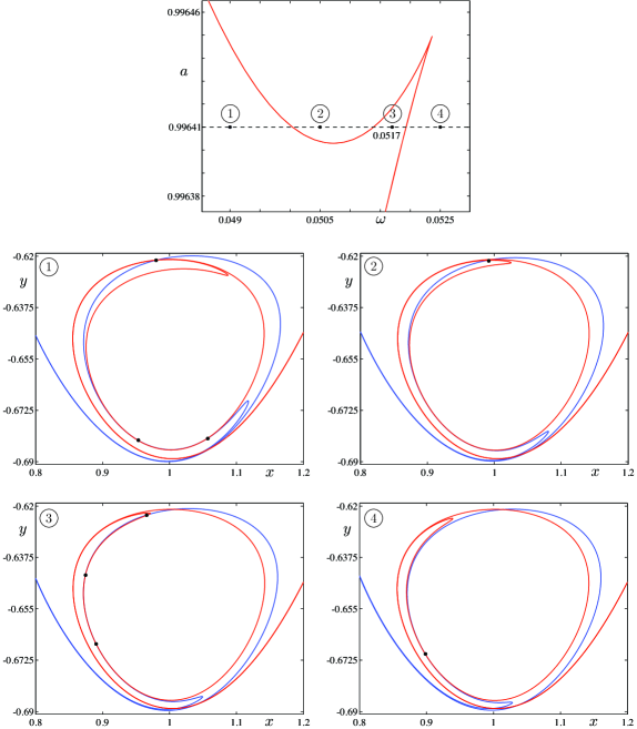
Figure 11: Evolution of the intersection points (black dots) between the curves representing $S_{a}^{\operatorname{\varepsilon}}$ and $S_{r}^{\operatorname{\varepsilon}}$ in a fixed cross-section through the folded node. Here, $a=0.99641$, $b=0.01$, and $\operatorname{\varepsilon}=0.05$. The values of $\omega$ are (1) 0.049, (2) 0.0505, (3) 0.0517, (4) 0.0525, as also labeled on the horizontal axis in the top frame. In the transition between frames (1) and (2), the lower two intersection points disappear. Between frames (2) and (3), two intersection points are created. Then, two disappear in the final transition shown, from (3) to (4)

5.2 Growth of LAOs from SAOs in the Secondary Canards

Along the continuation of the secondary canards, an orbit segment can ‘grow’ an LAO. This occurs in regions where the repelling slow manifold spirals backwards instead continuing to spiral inwards towards the weak canard. In Figure 12, we show the repelling slow manifold for $\overline{\omega}=0.3$ in the cross-section $\Sigma_{n}$; the direction of spiralling changes three times along this portion of the slow manifold, at the points labeled (b1), (b2), and (b3) in frame (a). Each direction reversal corresponds to the orbit growing a large-amplitude oscillation. In panels (b1), (b2), and (b3), we show the profiles of the computed solution segments at these events. Note that the first fold encountered (starting from the center of the spiral and going outwards) corresponds to the orbit segment having one SAO grow up to the size of an LAO (this occurs at the second fold), while the other SAOs stop growing in size.

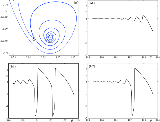
Figure 12: Repelling slow manifold reversing the direction of spiralling as successive LAOs appear in the orbit. Panels (b1), (b2), and (b3) show the solution profiles corresponding to three such events. Here, $a=0.9935,b=0.01,\omega=0.3$, and $\operatorname{\varepsilon}=0.05$.

Remark 5.

An important consequence of studying the curves of maximal canards and maximal torus canards in the parameter space of (1) is that they serve as the boundaries between different dynamic regimes of (1). As highlighted briefly by the graphical summary in the $(\omega,a)$ plane shown in Figure 4, the fvdP equation (1) exhibits small-amplitude oscillations (SAOs), large-amplitude or relaxation oscillations (LAOs), and mixed-mode oscillations (MMOs). The SAOs are the $\frac{2\pi}{\omega}$-periodic solutions generated when an attracting equilibrium of the unforced vdP equation (i.e., $b=0$) is subjected to a small-amplitude periodic forcing of frequency $\omega$ (Figure 13(a)). The LAOs occur when the equilibrium of the planar vdP equation sits on the middle branch of the cubic-shaped nullcline and the attractor of the system is a relaxation oscillation that alternates the trajectory between the outer branches of the cubic (Figure 13(f)). The MMOs feature SAOs superimposed on large-amplitude relaxation-type oscillations. Figure 4 shows that the MMOs become more robust for low-frequency forcing, just as was observed in numerical simulations of a rotated van der Pol-type model in [2].

Figure 13: Transition from SAOs to MMOs to LAOs in the forced vdP equation (1). The attractors of (1) are shown for $\operatorname{\varepsilon}=0.01$, $\omega=0.01$, and (a) $a=1.01$, (b) $a=0.9999$, (c) $a=0.999$, (d) $a=0.994$, (e) $a=0.991$, and (f) $a=0.987$.

6 The fvdP is a Normal Form for a Class of Systems Near Torus Canard Explosions

In this section, we prove that, under a number of natural conditions, a slow/fast system with two fast variables and one slow variable, which is subject to time-periodic forcing and for which the fast system possesses a generic fold of limit cycles, is equivalent to a system in which the fast component is given to lowest order by the forced van der Pol system (1). We consider systems with two fast variables and one slow variable of the following form:

$$\begin{split}\dot{x}&=f_{1}(x,y,z)\\ \dot{y}&=f_{2}(x,y,z)\\ \dot{z}&=\operatorname{\varepsilon}g(x,y,z),\qquad x,y,z\in\mathbb{R}.\end{split}$$ (33)

The fast system is

$$\begin{split}\dot{x}&=f_{1}(x,y,z)\\ \dot{y}&=f_{2}(x,y,z)\end{split}$$ (34)

in which $z$ is a parameter, and we make the following hypotheses about the fast system:

(H1) For $z=0$, there exists a non-degenerate periodic solution ${\tilde{\Gamma}}$; and, here by non-degenerate, we mean a periodic solution with finite period.

(H2) The Floquet multiplier of this periodic orbit at $z=0$ is one.

We prove the following theorem:

Theorem 6.1.

Given (H1), (H2), and a non-degeneracy assumption (see (70) below), system (33) is locally (in a small neighborhood of ${\tilde{\Gamma}}$) orbitally equivalent to

$$\begin{split}\dot{\rho}&=z-\rho^{2}+O(\rho^{3})+O(\operatorname{\varepsilon})\\ \dot{\theta}&=1\\ \dot{z}&=\operatorname{\varepsilon}\tilde{g}(\rho,\theta,z),\qquad\rho,z,\theta\in\mathbb{R},\end{split}$$ (35)

where $\tilde{g}$ is $2\pi$-periodic in $\theta$, and where $z$ and $\rho$ are small.

The fast subsystem of (35) has very similar dynamics to that of (1), however the slow system of the general systems may be much richer than the slow system of (1). We make a more detailed comparison between the full systems later in this section. We first analyze the fast systems.

We begin the proof of Theorem 6.1 with some preliminary transformations. On the basis of (H1), one may rectify the flow of (34) so that the periodic orbit becomes the unit circle. Next, using the coordinates

$$x=(1+r)\cos(\theta)\quad{\rm and}\quad y=(1+r)\sin(\theta),$$

one may transform (34) to

$$\begin{split}\dot{r}&=\tilde{f}_{1}(r,\theta,z)\\ \dot{\theta}&=\tilde{f}_{2}(r,\theta,z),\end{split}$$ (36)

where $\tilde{f}_{i}$ is $2\pi$ periodic in $\theta$, $\tilde{f}_{1}(0,\theta,0)=0$, and $\tilde{f}_{2}\neq 0$ in a neighborhood of $(0,\theta,0)$. Also, one may scale the time variable so that (36) becomes

$$\begin{split}\dot{r}&=F(r,\theta,z)\\ \dot{\theta}&=1,\end{split}$$ (37)

with $F=\tilde{f}_{1}/\tilde{f}_{2}$. This is a useful formulation of the fast system, and we work directly with this throughout the proof.

In order to analyse the dynamics of this system for small values of $r$, we expand:

$$F(r,\theta,z)=\psi_{0}(\theta,z)+r\psi_{1}(\theta,z)+r^{2}\psi_{2}(\theta,z)+\ldots+r^{N}\psi_{N}(\theta,z)+O(r^{N+1}).$$ (38)

Condition (H2) is now equivalent to

$$\int_{0}^{2\pi}\psi_{1}(\theta,0)d\theta=0,$$ (39)

because

$$\frac{\partial\bar{F}}{\partial r}(0,0)=0,$$

where the average of $F$ is defined as

$$\bar{F}(r,z)=\frac{1}{2\pi}\int_{0}^{2\pi}F(r,\theta,z)d\theta.$$

Also, to analyze the dynamics for small values of $r$, it is useful to introduce a new variable $\rho$ by

$$r=\phi_{0}+\rho e^{\phi_{1}}+\rho^{2}\phi_{2}+\ldots+\rho^{N}\phi_{N},\quad N\geq 2.$$ (40)

where $\phi_{i}$ are functions of $(\theta,z)$ to be determined.

The following lemma lies at the heart of the proof of this theorem:

Lemma 6.2.

There exists a choice of functions $\phi_{i}$, $i=1,\ldots,N$, in the coordinate change (40) and a function $G(\rho,z)$ such that, in the coordinates $(\rho,\theta)$, the fast system (37) has the form

$$\begin{split}\dot{\rho}&=G(\rho,z)+O(\rho^{N+1})\\ \dot{\theta}&=1.\end{split}$$ (41)

Remark 6.

Hypothesis (H2) is not needed for this lemma.

Proof. The proof is split into three steps. First, we consider the simplest case in which $N=1$ in (40). Next, we prove the Theorem for $N=2$, and finally we prove it for general $N$ in (40).

Step 1. With $N=1$, the relevant transformation (40) between $r$ and $\rho$ is:

$$r=\phi_{0}+\rho e^{\phi_{1}}.$$ (42)

Differentiating (42) with respect to time, substituting in (37), and Taylor expanding $F(\phi_{0}+\rho e^{\phi_{1}},\theta,z)$ about $\phi_{0}$, we obtain

$$\dot{\rho}=(-\phi_{0,\theta}+F(\phi_{0},\theta,z))e^{-\phi_{1}}+\rho(-\phi_{1,\theta}+F_{r}(\phi_{0},\theta,z))+O(\rho^{2}).$$ (43)

Hence, based on the form of the two terms in parentheses in the right member of this equation, we are naturally led to study the following system of two ordinary differential equations with two unknown parameters:

$$\begin{split}\phi_{0,\theta}&=F(\phi_{0},\theta,z)+\lambda_{0}e^{\phi_{1}}\\ \phi_{1,\theta}&=F_{r}(\phi_{0},\theta,z)+\lambda_{1}\end{split}$$ (44)

In this manner, proving the result for $N=1$ is now equivalent to finding $\lambda_{0}$ and $\lambda_{1}$ for which there exist $\phi_{0}$ and $\phi_{1}$ which are $2\pi$ periodic and which satisfy the equations (44).

According to general theory of differential equations, for every pair $(\lambda_{0},\lambda_{1})$, there exists a unique solution $(\phi_{0},\phi_{1})$ of (44) satisfying the initial conditions $\phi_{0}(0)=0$ and $\phi_{1}(0)=0$. Such solutions must satisfy the integral equations,

$$\begin{split}\phi_{0}(\theta)&=\int_{0}^{\theta}F(\phi_{0}(\nu),\nu,z)d\nu+\lambda_{0}\int_{0}^{\theta}e^{\phi_{1}(\nu)}d\nu\\ \phi_{1}(\theta)&=\int_{0}^{\theta}F_{r}(\phi_{0}(\nu),\nu,z)d\nu+\lambda_{1}\theta.\end{split}$$ (45)

Also, in terms of these integral equations, the conditions for periodicity are

$$\begin{split}0&=\int_{0}^{2\pi}F(\phi_{0}(\nu),\nu,z)d\nu+\lambda_{0}\int_{0}^{2\pi}e^{\phi_{1}(\nu)}d\nu\\ 0&=\int_{0}^{2\pi}F_{r}(\phi_{0}(\nu),\nu,z)d\nu+2\pi\lambda_{1}.\end{split}$$ (46)

Based on the above formulation of the integral equations, it is useful to define ${\cal H}\;:\;\mathbb{R}\times\mathbb{R}^{2}\to\mathbb{R}^{2}$, as follows:

$${\cal H}(z,\lambda_{0},\lambda_{1})=\left(\begin{array}[]{c}{\cal H}_{0}(z,\lambda_{0},\lambda_{1})\\ {\cal H}_{1}(z,\lambda_{0},\lambda_{1})\end{array}\right)=\left(\begin{array}[]{c}\int_{0}^{2\pi}F(\phi_{0}(\nu),\nu,z)d\nu+\lambda_{0}\int_{0}^{2\pi}e^{\phi_{1}(\nu)}d\nu\\ \int_{0}^{2\pi}F_{r}(\phi_{0}(\nu),\nu,z)d\nu+2\pi\lambda_{1}\end{array}\right).$$ (47)

Now, by the assumptions (H1) and (H2) (see (39)), $\lambda_{0}=0$, $\lambda_{1}=0$, and $z=0$ is a solution of (45) with $\phi_{0}=0$ and $\phi_{1,0}=\int_{0}^{\theta}F_{r}(0,\nu,0)d\nu$. We now verify that the assumptions of the Implicit Function Theorem are satisfied to show that there is a branch of nontrivial solutions emanating from this trivial solution. In particular, we verify that $D{\cal H}(0,0,0)$ is non-singular, by showing that ${\rm det}D{\cal H}(0,0,0)=(2\pi)^{2}$.

From the definition, we see that ${\cal H}_{1,\lambda_{1}}(0,0,0)=2\pi$. We will now show that ${\cal H}_{0,\lambda_{1}}(0,0,0)=0$ and ${\cal H}_{0,\lambda_{0}}(0,0,0)=2\pi$. To show that ${\cal H}_{0,\lambda_{1}}(0,0,0)=0$, we start with

$${\cal H}_{0,\lambda_{1}}(0,0,0)=\int_{0}^{2\pi}F_{r}(0,\theta,0)\phi_{0,\lambda_{1}}(\theta)d\theta.$$

Then, using (44), we obtain

$${\cal H}_{0,\lambda_{1}}(0,0,0)=\int_{0}^{2\pi}\frac{d}{d\theta}\phi_{0,\lambda_{1}}(\theta)d\theta=\phi_{0,\lambda_{1}}(2\pi)-\phi_{0,\lambda_{1}}(0).$$

By assumption (above formula (45)), $\phi_{0}(0)=0$ and $\phi_{1}(0)=0$ for $\lambda_{0}$ and $\lambda_{1}$. Hence, $\phi_{0,\lambda_{j}}(0)=0$ for $j=1,2$. Therefore, we conclude from (44) that $\phi_{0,\lambda_{1}}\equiv 0$, so that this entry of the Jacobian of ${\cal H}$ vanishes, as claimed.

Next, we show that ${\cal H}_{0,\lambda_{0}}(0,0,0)=2\pi$. By an argument similar to the above,

$${\cal H}_{0,\lambda_{0}}(0,0,0)=\phi_{0,\lambda_{0}}(2\pi)-\phi_{0,\lambda_{0}}(0)=\phi_{0,\lambda_{0}}(2\pi).$$

Therefore, from (44), we obtain

$$\frac{d}{d\theta}\left(\phi_{0,\lambda_{0}}\right)=F_{r}(0,\theta,0)\phi_{0,\lambda_{0}}+e^{\phi_{1}}.$$ (48)

Observe that, for $\lambda_{0}=0$ and $\lambda_{1}=0$, we have $d\phi_{1}/d\theta=F_{r}(0,\theta,0)$. Hence, (48) is equivalent to

$$\frac{d}{d\theta}\left(\phi_{0,\lambda_{0}}\right)=\frac{d\phi_{1}}{d\theta}\phi_{0,\lambda_{0}}+e^{\phi_{1}},$$ (49)

from which it follows that

$$\frac{d}{d\theta}\left(\phi_{0,\lambda_{0}}e^{-\phi_{1}}\right)=1.$$

Finally, since $\phi_{0,\lambda_{0}}(0)=0$, it follows from (39) that $\phi_{0,\lambda_{0}}(2\pi)=2\pi$. Therefore,

$$\det(D{\cal H}(0,0))=(2\pi)^{2},$$

and by the Implicit Function Theorem there is a branch of periodic solutions $\phi_{0}$ and $\phi_{1}$ for each $(\lambda_{0},\lambda_{1})$ sufficiently small, emanating from the trivial solution. This completes the proof of the Lemma for the case $N=1$.

Step 2. We now show that the lemma holds for $N=2$ in (40). All quantities are expanded up to and including $\rho^{2}$. For the vector field $F$, we have

$$F(r,\theta,z)=F(\phi_{0},\theta,z)+\rho F_{r}(\phi_{0},\theta,z)e^{\phi_{1}}+\rho^{2}(F_{r}(\phi_{0},\theta,z)\phi_{2}+\frac{1}{2}F_{rr}(\phi_{0},\theta,z)e^{2\phi_{1}}).$$ (50)

Also, differentiating (40) for $N=2$ with respect to $t$, we find

$$\dot{r}=\dot{\rho}(e^{\phi_{1}}+2\rho\phi_{2})+\phi_{0,\theta}+\rho e^{\phi_{1}}\phi_{1,\theta}+\rho^{2}\phi_{2,\theta}.$$ (51)

Hence, combining (50) and (51), we get

$$\begin{split}\dot{\rho}(1+2\rho\phi_{2}e^{-\phi_{1}})=&(-\phi_{0,\theta}+F(\phi_{0},\theta,z))e^{-\phi_{1}}+\rho(-\phi_{1,\theta}+F_{r}(\phi_{0},\theta,z))\\ &+\rho^{2}(-\phi_{2,\theta}+F_{r}(\phi_{0},\theta,z)\phi_{2}+\frac{1}{2}F_{rr}(\phi_{0},\theta,z)e^{2\phi_{1}})e^{-\phi_{1}}.\end{split}$$ (52)

Now, after multiplying both sides of (52) by $(1+2\rho\phi_{2}e^{-\phi_{1}})^{-1}$, we examine the structure of the terms at each order of $\rho^{0},\rho^{1},$ and $\rho^{2}$. This suggests that we analyze the following system of differential equations:

$$\begin{split}\phi_{0,\theta}&=F(\phi_{0},\theta,z)+\lambda_{0}e^{\phi_{1}}\\ \phi_{1,\theta}&=F_{r}(\phi_{0},\theta,z)-2\lambda_{0}\phi_{2}e^{-\phi_{1}}+\lambda_{1}\\ \phi_{2,\theta}&=F_{r}(\phi_{0},\theta,z)\phi_{2}+\frac{1}{2}F_{rr}(\phi_{0},\theta,z)e^{2\phi_{1}}-2\lambda_{1}\phi_{2}+\lambda_{2}e^{\phi_{1}}.\end{split}$$ (53)

The first equation here is equivalent to the first equation in (44); the second has an additional term due to $\phi_{2}$; and, the third is new. If we can find a branch of nontrivial solutions of this system, then we can transform the general fast system into the desired form up to and including ${\cal O}(\rho^{2})$.

As above, we look for $2\pi$ periodic solutions. However, before extending the definition of ${\cal H}$, we rewrite the third component of (53) as follows:

$$\frac{d}{d\theta}\left(\phi_{2}e^{-\phi_{1}}\right)=\frac{1}{2}F_{rr}(\phi_{0},\theta,z)e^{\phi_{1}}+2\lambda_{0}\phi_{2}^{2}e^{-2\phi_{1}}-3\lambda_{1}\phi_{2}e^{-\phi_{1}}+\lambda_{2}.$$ (54)

Now, we define ${\cal H}\;:\;\mathbb{R}\times\mathbb{R}^{3}\to\mathbb{R}^{3}$ in a manner similar to that employed in Step 1:

$$\begin{split}&{\cal H}(z,\lambda_{0},\lambda_{1},\lambda_{2})=\left(\begin{array}[]{c}{\cal H}_{0}(z,\lambda_{0},\lambda_{1},\lambda_{2})\\ {\cal H}_{1}(z,\lambda_{0},\lambda_{1},\lambda_{2})\\ {\cal H}_{2}(z,\lambda_{0},\lambda_{1},\lambda_{2})\end{array}\right)=\\ &\left(\begin{array}[]{l}\int_{0}^{2\pi}F(\phi_{0}(\nu),\nu,z)d\nu+\lambda_{0}\int_{0}^{2\pi}e^{\phi_{1}(\nu)}d\nu\\ \int_{0}^{2\pi}(F_{r}(\phi_{0}(\nu),\nu,z)-2\lambda_{0}\phi_{2}(\nu)e^{-\phi_{1}(\nu)})d\nu+2\pi\lambda_{1}\\ \int_{0}^{2\pi}(\frac{1}{2}F_{rr}(\phi_{0}(\nu),\nu,z)e^{\phi_{1}(\nu)}+2\lambda_{0}\phi_{2}(\nu)^{2}e^{-2\phi_{1}(\nu)}-3\lambda_{1}\phi_{2}(\nu)e^{-\phi_{1}(\nu)}+\lambda_{2})d\nu\end{array}\right).\end{split}$$ (55)

We analyse ${\cal H}$ in much the same manner as in Step 1. Observe that, at $z=0$, we have $\lambda_{0}=0$ and $\lambda_{1}=0$. However, $\lambda_{2}$ is in general given by

$$\lambda_{2}=-\frac{1}{2\pi}\int_{0}^{2\pi}\frac{1}{2}F_{rr}(0,\nu,0)e^{\phi_{1}(\nu)}d\nu,$$

and not zero.

We now show that the off-diagonal elements of the Jacobian of ${\cal H}$ vanish. First, an argument similar to that used in Step 1 shows that ${\cal H}_{0,\lambda_{1}}(0,0,0,\lambda_{2,0})=0$. We also need to show that ${\cal H}_{0,\lambda_{2}}(0,0,0,\lambda_{2,0})=0$ and ${\cal H}_{1,\lambda_{2}}(0,0,0,\lambda_{2,0})=0$. To this end, we prove that $\phi_{0,\lambda_{2}}(0,0,0,\lambda_{2,0})\equiv 0$ and $\phi_{1,\lambda_{2}}(0,0,0,\lambda_{2,0})\equiv 0$, because then the identities ${\cal H}_{0,\lambda_{2}}(0,0,0,\lambda_{2,0})=0$ and ${\cal H}_{1,\lambda_{2}}(0,0,0,\lambda_{2,0})=0$ follow in a straightforward way. We carry out the proof for $\phi_{0,\lambda_{2}}$; the argument for $\phi_{1,\lambda_{2}}$ is similar. Differentiating the first equation in (53) with respect to $\lambda_{2}$ and using the fact that $\lambda_{0}\;|_{z=0}=0$, we obtain

$$\frac{d\phi_{0,\lambda_{2}}|_{z=0}}{d\theta}=F_{r}(0,\theta,0)\phi_{0,\lambda_{2}}|_{z=0}.$$ (56)

The claim now follows from the assumption $\phi_{0}(0,z,\lambda_{0},\lambda_{1},\lambda_{2})\equiv 0$.

Based on the above analysis, it follows that

$$\det(D{\cal H}(0,0,0,0))={\cal H}_{0,\lambda_{0}}(0,0,0,0){\cal H}_{1,\lambda_{1}}(0,0,0,0){\cal H}_{2,\lambda_{2}}(0,0,0,0),$$

and an argument similar to the one used in Step 1 shows that this determinant is nonzero. In particular, ${\cal H}_{0,\lambda_{0}}(0,0,0,0)$ and ${\cal H}_{1,\lambda_{1}}(0,0,0,0)$ are both $2\pi$ by a similar calculation. To show that also ${\cal H}_{2,\lambda_{2}}(0,0,0,0)=2\pi$, we differentiate the third component in (55) to obtain

$${\cal H}_{2,\lambda_{2}}(0,0,0,0)=\int_{0}^{2\pi}d\nu=2\pi.$$

Hence, we may again use the Implicit Function Theorem to conclude that there exists a branch of nontrivial solutions of (53), and the system may be put in the desired form up to and including terms of $\rho^{2}$. This completes the proof of Lemma 6.2 for the case $N=2$.

Step 3. In this third and final step of the proof, we show that the lemma holds for general $N$ in (40). We begin by writing

$$F(r,\theta,z)=\sum_{j=0}^{N}\rho^{j}F_{j}(\phi_{0},\phi_{1},\ldots,\phi_{N},\theta,z)+O(\rho^{N+1}),$$ (57)

where $N>2$ is a natural number and $r$ and $\rho$ are related by formula (40) associated to this choice of $N$. For each $j$, the functions $F_{j}$ are complicated expressions involving $\phi_{0}$, $\phi_{1}$, $\ldots$, $\phi_{j}$. To simplify the notation, we write $\Phi_{j}=(\phi_{0},\phi_{1},\ldots,\phi_{j})$. We will give a more precise description of the functions $F_{j}$ below. The equivalent of (52) is now

$$\begin{split}\dot{\rho}(1+\sum_{l=2}^{N}l\rho^{l-1}\phi_{l}e^{-\phi_{1}})=&(-\phi_{0,\theta}+F(\phi_{0},\theta,z))e^{-\phi_{1}}+\rho(-\phi_{1,\theta}+F_{r}(\phi_{0},\theta,z))\\ &+\sum_{j=2}^{N}\rho^{j}(-\phi_{j,\theta}+F_{j}(\Phi_{j},\theta,z))e^{-\phi_{1}}.\end{split}$$ (58)

Let $\alpha_{0}=1$ and for each $j\geq 1$ set

$$\alpha_{j}(\phi_{0},\ldots,\phi_{n})=\frac{1}{j!}\partial^{j}_{\rho}\left(\frac{1}{1+\sum_{l=2}^{n}l\rho^{l-1}\phi_{l}e^{-\phi_{1}}}\right)\big{|}_{\rho=0}.$$

Note that, for given $j$, $\alpha_{j}$ depends on $\phi_{0},\phi_{1},\ldots,\phi_{j+1}$. We also write

$$\begin{split}E_{0}&=(-\phi_{0,\theta}+F(\phi_{0},\theta,z))e^{-\phi_{1}}\\ E_{1}&=-\phi_{1,\theta}+F_{r}(\phi_{0},\theta,z)\\ E_{2}&=(-\phi_{2,\theta}+F_{2}(\Phi_{2},\theta,z))e^{-\phi_{1}}\\ &\vdots\\ E_{N}&=(-\phi_{N,\theta}+F_{N}(\Phi_{N},\theta,z))e^{-\phi_{1}}.\end{split}$$ (59)

It follows that (58) maay be written in the following compact and insightful manner:

$$\dot{\rho}=\sum_{l=0}^{N}\rho^{l}\left(\sum_{j=0}^{l}\alpha_{j}E_{l-j}\right).$$ (60)

We now define the set of equations

$$\begin{split}E_{0}&=\lambda_{0}\\ E_{1}+\alpha_{1}E_{0}&=\lambda_{1}\\ E_{2}+\alpha_{1}E_{1}+\alpha_{2}E_{0}&=\lambda_{2}\\ &\vdots\\ \sum_{j=0}^{N}\alpha_{j}E_{N-j}&=\lambda_{N}.\end{split}$$ (61)

This enables us to rewrite 59 as follows:

$$\begin{split}E_{0}&=\lambda_{0}\\ E_{1}&=\lambda_{1}-\alpha_{1}\lambda_{0}\\ E_{2}&=\lambda_{2}-\alpha_{1}\lambda_{1}+(\alpha_{1}^{2}-\alpha_{2})\lambda_{0}\\ &\vdots\\ E_{N}&=\sum_{j=0}^{N}\beta_{j}\lambda_{N-j},\end{split}$$ (62)

where $\beta_{0}=1$ and $\beta_{1},\ldots,\beta_{N}$ are coefficients depending on $\alpha_{0},\ldots,\alpha_{N}$. Moreover, $\beta_{j}$ depends on $\alpha_{0},\ldots,\alpha_{j}$ only. Therefore, we have arrived at the following system of differential equations:

$$\begin{split}\phi_{0,\theta}&=F(\phi_{0},\theta,z)+\lambda_{0}e^{\phi_{1}}\\ \phi_{1,\theta}&=F_{r}(\phi_{0},\theta,z)+\lambda_{1}-\alpha_{1}\lambda_{0}\\ \phi_{2,\theta}&=F_{2}(\Phi_{2},\theta,z)+(\lambda_{2}-\alpha_{1}\lambda_{1}+(\alpha_{1}^{2}-\alpha_{2})\lambda_{0})e^{\phi_{1}}\\ &\vdots\\ \phi_{N,\theta}&=F_{N}(\Phi_{N},\theta,z)+\left(\sum_{j=0}^{N}\beta_{j}\lambda_{N-j}\right)e^{\phi_{1}},\end{split}$$ (63)

which is the analog for general $N$ of the systems of differential equations (44) for $N=1$ and (53) for $N=2$.

Before defining ${\cal H}$, we rewrite (63) in a manner similar to that which was used above to rewrite (53) (recall also (54)). Noting that

$$F_{j}(\Phi_{j},\theta,z)=F_{r}(\phi_{0},\theta,z)\phi_{j}+{\cal R}(\Phi_{j-1}),$$

we replace the $j$th equation in (63) by

$$\frac{d}{d\theta}\left(\phi_{j}e^{-\phi_{1}}\right)={\cal R}(\Phi_{j-1})e^{-\phi_{1}}-(\lambda_{1}-\alpha_{1}\lambda_{0})\phi_{j}e^{-\phi_{1}}+\left(\sum_{l=0}^{j}\beta_{l}\lambda_{j-l}\right).$$ (64)

We will now define the function ${\cal H}$ in a manner analogous to (47) and (55) used in STeps 1 and 2, respectively, for the cases $N=1$ and $N=2$. We let

$$(\phi_{0}(\theta,z,\lambda_{1},\ldots,\lambda_{N}),\phi_{1}(\theta,z,\lambda_{1},\ldots,\lambda_{N}),\ldots,\phi_{N}(\theta,z,\lambda_{1},\ldots,\lambda_{N}))$$

be the solutions of (63) depending on the parameters $z$ and $\lambda_{0},\ldots,\lambda_{N}$ that satisfy the initial conditions $\phi_{j}(0,z,\lambda_{1},\ldots,\lambda_{N})=0$, $j=0,1,\ldots,N$. Further, we let ${\cal H}_{0}$, ${\cal H}_{1}$, and ${\cal H}_{2}$ be defined as in Step 2, and let

$${\cal H}_{j}(z,\lambda_{0},\lambda_{1},\ldots,\lambda_{N})=\int_{0}^{2\pi}\left({\cal R}(\Phi_{j-1})e^{-\phi_{1}}-(\lambda_{1}-\alpha_{1}\lambda_{0})\phi_{j}e^{-\phi_{1}}+\sum_{l=0}^{j}\beta_{l}\lambda_{j-l}\right)d\nu,\qquad j=2,3,\ldots N.$$ (65)

We first argue that we can solve the set of equations ${\cal H}_{j}(0,\lambda_{0},\ldots,\lambda_{N})$, $j=0,1,\ldots,N$, for a unique $N$-tuple $(\lambda_{0,0},\lambda_{1,0},\ldots,\lambda_{N,0})$. Note that $\lambda_{0,0}=0$ and $\lambda_{1,0}=0$, by the same analysis used in Step 2. Hence,

$$\sum_{k=0}^{j}\beta_{k}\lambda_{j-k}|_{z=0}=\sum_{k=0}^{j-2}\beta_{k}\lambda_{j-k}|_{z=0}.$$

We argue by induction. Suppose that $\lambda_{0,0},\ldots,\lambda_{j-1,0}$ and the corresponding $\phi_{0},\ldots,\phi_{j-1}$ are determined. Note that $\lambda_{j,0}$ must satisfy

$$\lambda_{j,0}=-\int_{0}^{2\pi}\left({\cal R}(\Phi_{j-1})e^{-\phi_{1}}+\sum_{l=1}^{j-2}\beta_{l}\lambda_{j-l,0}\right)d\nu.$$ (66)

Since the right member of (66) depends only on $\lambda_{0},\ldots,\lambda_{j-1}$ and $\phi_{0},\ldots,\phi_{j-1}$ the value of $\lambda_{j,0}$ is uniquely determined. Similarly, knowing $\lambda_{j,0}$, we can solve (64) for $\phi_{j}$ using (64) due to the fact that $\lambda_{0}=\lambda_{1}=0$, so that right member of (64) depends only on $\lambda_{0},\ldots,\lambda_{j-1}$ and $\phi_{0},\ldots,\phi_{j-1}$. Hence, $\phi_{j}$ is uniquely determined.

We now prove that $D_{\lambda_{0},\ldots,\lambda_{N}}{\cal H}(0,\lambda_{0,0},\ldots,\lambda_{N,0})$ is non-singular. First, we prove that $\phi_{j,\lambda_{k}}|_{z=0}=0$ for any $j\in\{0,\ldots,N-1\}$ and $k\in\{j+1,\ldots,N\}$. The argument for $j=0$ and $j=1$ is analogous as in the case of $n=2$. For general $j$, we proceed by induction, assuming that the claim holds for $0,1,\ldots,j-1$. The argument is, again, similar to that used in the case $N=2$. We differentiate (64) with respect to $\lambda_{k}$ and use the induction assumption, the fact that $\beta_{j}$ is independent of $\phi_{l}$ for any $l>j+1$, and the fact that $\lambda_{0,0}=\lambda_{1,0}=0$. This gives

$$\frac{d}{d\theta}\phi_{j,\lambda_{k}}(0,\lambda_{0,0},\ldots,\lambda_{N,0})=0.$$ (67)

By assumption, $\phi_{j}(0,z,\lambda_{0},\ldots,\lambda_{N})\equiv 0$. Hence, the claim follows. Now, differentiating (65) and using a similar procedure, we obtain ${\cal H}_{j,\lambda_{k}}(0,\lambda_{0,0},\ldots,\lambda_{N,0})=0$ for $j\in\{0,\ldots,N-1\}$ and $k\in\{j+1,\ldots,N\}$.

It remains to prove that ${\cal H}_{j,\lambda_{j}}(0,\lambda_{0,0},\ldots,\lambda_{N,0})\neq 0$ for $j\in\{0,\ldots,N\}$. The proof for $j=0$ and $1$ is as above. Let $j>1$. Again by differentiating (65), now with respect to $\lambda_{j}$, and arguing analogously as above, we obtain

$${\cal H}_{j,\lambda_{j}}(0,\lambda_{0,0},\ldots,\lambda_{N,0})=\int_{0}^{2\pi}d\nu=2\pi.$$ (68)

We can now apply the Implicit Function Theorem to obtain the functions $\lambda_{0}(z),\ldots,\lambda_{j}(z)$ as required. This completes the third (and final) step of the proof of the lemma.

QED

Proof of Theorem 6.1 If we apply the sequence of transformations leading to (41) to system (33), we obtain a system of the form

$$\begin{split}\dot{\rho}&=G(\rho,z)+O(\rho^{N+1})+O(\operatorname{\varepsilon})\\ \dot{\theta}&=1\\ \dot{z}&=\operatorname{\varepsilon}\tilde{g}(\rho,\theta,z,\operatorname{\varepsilon}).\end{split}$$ (69)

with

$$G(\rho,z)=\sum_{j=0}^{N-1}\lambda_{j}(z)\rho^{j}$$

and the coefficient functions are as introduced in the proof of Lemma 6.2. In particular hypotheses (H1) and (H2) imply $\lambda_{0}(0)=0$ and $\lambda_{1}(0)=0$. We now formulate the additional degeneracy assumptions in terms of the functions $\lambda_{j}$. We will assume that $N\geq 3$.

$$\begin{split}\frac{d\lambda_{0}}{dz}\left(0\right)&\neq 0.\\ \lambda_{2}(0)&\neq 0.\end{split}$$ (70)

If (70) holds in addition to (H1) and (H2) we replace the variable $z$ by $\tilde{z}=\lambda_{0}(z)$ and perform scalings and translations to arrive at (35), taking $\operatorname{\varepsilon}$ sufficiently small as necessary. QED

We now make some remarks relating the normal form equation (35) derived in this section and the forced van der Pol (1). Clearly, the fast subsystems are similar. If in addition to (70) we assume that $\lambda_{3}(0)\neq 0$ and make some assumptions about the signs of the coefficients, then the two fast systems are the same to lowest order (up to a simple transformation). The situation with the slow equation is more complicated. In systems with time-periodic forcing, we have shown that (1) is a normal form. Moreover, because forced systems are not generic in the larger class of general slow/fast dynamical systems, we expect the dynamics in this larger class to be even richer. In addition, if we assume that $\tilde{g}(0,\theta_{0},0,0)=0$ for some $\theta_{0}\in[0,\,2\pi)$ then we may obtain some canard dynamics. In general these slow/fast systems will have folded singularities and associated canard dynamics.

7 Conclusions and Discussion

In this article, we have established the existence of a number of different types of canard solutions of the forced van der Pol equation (1) across the entire range of forcing frequencies $\omega>0$. Most interestingly, we have found numerically that the families of primary maximal canards and maximal torus canards are organised along single branches in parameter space. In the low-frequency regime ($\omega={\cal O}(\operatorname{\varepsilon})$), Theorem 1.1 demonstrates the existence of the primary maximal canards of the FSN I points and establishes that formula (2) gives the loci of the folds of the primary maximal canards in the $(a,b,\overline{\omega})$ parameter space with $b={\cal O}(\sqrt{\operatorname{\varepsilon}})$. In the intermediate-frequency ($\omega={\cal O}(\sqrt{\operatorname{\varepsilon}})$) and high-frequency regime ($\omega={\cal O}(1)$), Theorem 1.2 and Corollary 1.3, respectively, establish the existence of maximal torus canards as well as the formulas (3) and (4), which explicitly give the locations of the folds of the maximal torus canards in the $(a,b,\omega)$ parameter space with $b={\cal O}(\operatorname{\varepsilon})$. These maximal torus canards lie precisely in the intersection of the persistent critical manifolds of attracting limit cycles and of repelling limit cycles. They are the analogs in one-higher-dimension of the maximal headless ducks of the unforced van der Pol equation, see for example [3, 19, 21]. Moreover, they are similar to the folds of maximal torus canards observed earlier in a rotated system of ven der Pol type, see Figure 5 in [2].

It was also shown that these analytical results are all representations of the same formula (6) that holds across the entire range of forcing frequencies $\omega>0$ for the appropriate values of $b$, and that these formulas agree well with the results obtained from numerical continuations over the parameter regions in which they apply. Moreover, in the limit $\omega\to\infty$, the torus canards appear to be rotated copies of the limit cycle canards that exist in the planar unforced van der Pol equation, and the interval of $a$ values for which the maximal torus canards exist shrinks to the value $a_{c}(\operatorname{\varepsilon})=1-\frac{\operatorname{\varepsilon}}{8}$ at which the maximal headless duck solution exists in the unforced equation, recall [1, 3, 6, 19, 21].

It is worth noting that the analytical results presented here for the torus canards of (1) agree with and expand upon by the general topological analysis presented in Section 6 of [8]. There, fast-slow systems with two fast variables and one slow variable were studied in which there is a torus canard explosion in the transition regime from stable periodic spiking (tonic spiking) to bursting, and examples were given, including of the Hindmarsh-Rose equation, the Morris-Lecar-Terman model, and the Wilson-Cowan-Izhikevich system. In particular, it was shown using topological arguments that there must be a sequence of torus canards in these transition regimes in order to satisfy the property of continuous dependence of solutions on parameters. The topological analysis presented in [8] is the analog in one higher dimension of the topological analysis first used in [3] to establish the existence of an explosion of limit cycle canards in the transition between asymptotically stable solutions and full-blown relaxation oscillations in the unforced, planar van der Pol equation.

In this article, we also studied the branches of the secondary maximal canards, which exist in the low-frequency regime in (1). Secondary canards lie close to the primary strong canard for most of their lengths, and in addition they make finitely many loops near the bottom of $\Gamma$, recall Figure 7. They are indexed by the number of loops and by the height in the $y$ variable of the jumps from the repelling slow manifold back to the attracting slow manifold. We showed how the dynamics of these secondary canards changes as the parameters change along the fold curves, and we identified the mechanism by which these branches turn around well before they get into the high-frequency regime. In particular, the turning points correspond precisely to the parameter values at which the fold curve of maximal canards is crossed and two intersection points of the attracting and repelling slow manifolds are created (or annihilated). In addition, we identified how new LAO segments are added to the secondary canard solutions at points at which the direction of spiralling of the repelling slow manifold is reversed, recall Figure 9.

Finally, we proved that the fvdP equation (1) is a normal form for a class of slow/fast systems with two fast variables and one slow variable, which possess a non-degenerate fold of limit cycles in the fast system and which exhibit the torus canard explosion phenomenon. Thus, the methods and results obtained here for (1) extend naturally to a large class of slow/fast systems with single-frequency time-periodic forcing.

To conclude this article, we discuss a number of topics related to the canard solutions of the fvdP (1). First, the fold curves of the primary maximal canards in the low-frequency regime and the fold curves of the maximal torus canards in the intermediate- and high-frequency regimes together serve as the boundary of the MMO regime in (1), recall Figures 4 and 13.

Second, there are many different branches of resonance curves, curves of torus bifurcations, saddle-nodes of periodic orbits, period-doubling curves of periodic orbits, and so forth, all of which lie in the interior of the MMO region in parameter space. These bifurcation curves play important roles as the boundaries between orbit segments with different numbers of SAOs and LAOs. These are the subject of ongoing research.

Appendix A Proof of the Existence of a Torus Bifurcation

In this appendix, we consider the forced vdP oscillator (1) subject to high-frequency forcing ($\omega=\mathcal{O}(1)$). In this case, $y$ is the only slow variable, and there is no critical manifold. As such, the fast dynamics are dominant throughout the phase space, and system (1) can be interpreted as a regularly perturbed, non-autonomous problem.

We establish the existence of a torus bifurcation using second-order averaging and equivariant normal form theory in Section A.1, and we present the asymptotics of the torus bifurcation parameter value $a_{\rm TB}(b,\omega,\varepsilon)$ in Section A.2.

A.1 Second-Order Averaging and a Torus Bifurcation in the Regime $\omega=\mathcal{O}(1)$

In this section, we perform a standard second-order averaging analysis of system (1) and use equivariant normal form theory in the regime $\omega=\mathcal{O}(1)$ to demonstrate that there exists a smooth function $a=a_{\rm TB}(b,\omega,\varepsilon)$ at which the system possesses a torus bifurcation in which a stable two-torus is born. First, we change variables so that the fold is located at the origin: $({\tilde{x}},{\tilde{y}})=(1-x,y+\frac{2}{3})$ and $\alpha=a-1$. The forced vdP equation transforms to

$$\tilde{x}^{\prime} =-{\tilde{y}}+{\tilde{x}}^{2}-\frac{1}{3}{\tilde{x}}^{3}$$

$${\tilde{y}}^{\prime} =\varepsilon\left({\tilde{x}}+\alpha+b\cos\theta\right)$$

$$\theta^{\prime} =\omega.$$

Then, to carry out the second-order averaging analysis, it is natural to use the following scaling, which comes from the central chart of the desingularization, or blow-up, analysis used in Section 4 and in [36]:

$${\tilde{x}}=\sqrt{\operatorname{\varepsilon}}\,\overline{x},\quad{\tilde{y}}=\operatorname{\varepsilon}\overline{y},\quad b=\sqrt{\operatorname{\varepsilon}}\,\overline{b},\quad\alpha=\sqrt{\operatorname{\varepsilon}}\,\overline{\alpha},$$

and to rescale time by $t\longrightarrow\omega t$. Hence, after dropping the bars, the system has the following non-autonomous form:

$$\begin{split}\dot{x}&=\frac{\delta}{\omega}\left(-y+x^{2}\right)-\frac{\delta^{2}}{3\omega}x^{3}\\ \dot{y}&=\frac{\delta}{\omega}\left(x+\alpha+b\cos(t_{0}+t)\right),\end{split}$$ (71)

where $\delta=\sqrt{\operatorname{\varepsilon}}$. The choice of $t_{0}$ has no effect on the analysis.

Next, we apply the near-identity change of variables used in second-order averaging [49], so that system (71) transforms into

$$\begin{split}\dot{\xi_{1}}&=\frac{\delta}{\omega}\left(-\xi_{2}+\xi_{1}^{2}\right)-\frac{\delta^{2}}{3\omega}\xi_{1}^{3}+\tilde{G}(\xi_{1},\xi_{2},t,\delta)\\ \dot{\xi_{2}}&=\frac{\delta}{\omega}\left(\xi_{1}+\alpha\right)+O(\delta^{3}),\end{split}$$ (72)

with $\tilde{G}(\xi_{1},\xi_{2},t,\delta)=O(\delta^{3})$. We label (72) as the ‘intermediate’ system; it is smoothly conjugate to the original system.

We are interested in the averaged system,

$$\begin{split}\dot{\bar{x}}&=\frac{\delta}{\omega}\left(-\bar{y}+\bar{x}^{2}\right)-\frac{\delta^{2}}{3\omega}\bar{x}^{3}\\ \dot{\bar{y}}&=\frac{\delta}{\omega}\left(\bar{x}+\alpha\right).\end{split}$$ (73)

This system has a unique $S^{1}$ equivariant normal form [25] due to its symmetry properties. Moreover, the time-$T$ map of this normal form must be the $S^{1}$ normal form of the time-$T$ map, since the two operations commute and since $S^{1}$ equivariant normal forms are unique. Let $\bar{\mathfrak{s}}$ denote the Poincare map of this normal form. At $\alpha=0$, the eigenvalues of the map $\bar{\mathfrak{s}}$ satisfy the non-resonance condition: they are not equal to the first four strong resonant eigenvalues. Also, the second Liapunov coefficient is negative; in fact, for the averaged system, the second Liapunov coefficient is known to be $K\delta$, where $K<0$ is a constant. Hence, at $\alpha=0$, the map $\bar{\mathfrak{s}}$ satisfies the basic hypotheses of the Hopf bifurcation for maps; see conditions A) and B), respectively, and Theorem 2 of [38]. Therefore, at $\alpha=0$, the map $\bar{\mathfrak{s}}$ undergoes a non-degenerate, supercritical Hopf bifurcation in which a normally-hyperbolic invariant circle is created. Hence, one also sees directly that the averaged system (73) undergoes a torus bifurcation at $\alpha=0$ in which the limit cycle becomes unstable and a stable invariant torus is created.

We now demonstrate that the full system (71) undergoes a torus bifurcation at some $\alpha_{\rm TB}$ near $\alpha=0$, in which a stable invariant torus is created. In particular, we show that the Poincare map $\mathfrak{s}$ of the full system (71) possesses an invariant circle $\delta$-close to the one of $\bar{\mathfrak{s}}$.

First, we observe that the same near-identity coordinate change employed above to put the averaged system (73) into its $S^{1}$ equivariant normal form also puts the intermediate system (72) into its $S^{1}$ equivariant normal form, up to and including ${\cal O}(\delta^{2})$. Let $\mathfrak{s}_{i}(z)$ denote the Poincare map of this normal form. Again, this map must be the time-$T$ map of the normal form, due to uniqueness in the $S^{1}$ equivariant case. Next, we observe that, by standard second-order averaging theory, the Poincare maps are close, i.e., on time intervals of length $\mathcal{O}(1/\delta)$,

$$\left|\mathfrak{s}_{i}(z)-\bar{\mathfrak{s}}(z)\right|={\cal O}(\delta).$$

In fact, for each $\alpha$ sufficiently small, the map $\mathfrak{s}_{i}$ is part of exactly the type of one-parameter family of maps studied in [38], with the map of the averaged system being the ‘unperturbed’ map. Hence, for some $\alpha$ near $\alpha=0$, the map $\mathfrak{s}_{i}$ also undergoes a non-degenerate, super-critical Hopf bifurcation in which a normally-attracting invariant circle is created.

Finally, we observe that the time-$T$ maps $\mathfrak{s}$ and $\mathfrak{s}_{i}$ are smoothly conjugate. Hence, it follows that the map $\mathfrak{s}$ of the original system (71) also has a non-degenerate Hopf bifurcation, and therefore that the original vector field (71) has a torus bifurcation at some $\alpha_{\rm TB}$ near zero, in which an attracting invariant torus is created. This concludes the demonstration.

Remark 7.

One boundary of the parameter $\alpha$ for the existence of an invariant torus for the full system is given by the birth of the canard regime.

A.2 Asymptotic Expansion of $a_{\rm TB}(b,\omega,\varepsilon)$

In this section, we present the asymptotic expansion of $a=a_{TB}(b,\omega,\operatorname{\varepsilon})$ for small $b$. The unforced vdP equation has an equilibrium at $(x,y)=(a,f(a))$, which undergoes a Hopf bifurcation at $a=1$. This corresponds to a periodic orbit of (1) at $b=0$ which undergoes a torus bifurcation at $a=1$. We seek periodic solutions of (1) as an asymptotic series in $b$, i.e., let

$$x(t)=\sum_{k=0}^{\infty}b^{k}x_{k}(t),\quad y(t)=\sum_{k=0}^{\infty}b^{k}y_{k}(t).$$

Substitution into (1) yields

$$\dot{x}_{0} =y_{0}-f(x_{0}),$$

$$\dot{y}_{0} =\operatorname{\varepsilon}(a-x_{0}),$$

at leading order, which is the planar van der Pol equation. This has an equilibrium at $(x,y)=(a,f(a))$. The $\mathcal{O}(b^{1})$ system is

$$\dot{x}_{1} =y_{1}-f^{\prime}(x_{0})\,x_{1},$$

$$\dot{y}_{1} =\operatorname{\varepsilon}(-x_{1}+\cos\omega t).$$

The $\mathcal{O}(b^{1})$ system is linear with solutions that are linear combinations of $\cos\omega t,\sin\omega t$, and $\exp(\lambda t)$, where $2\lambda=1-a^{2}\pm\sqrt{(1-a^{2})^{2}-4\operatorname{\varepsilon}}$.

Remark 8.

Note that when $a=1$ and $\omega=\sqrt{\operatorname{\varepsilon}}$, there is a resonance.

When a damped oscillator is driven with a periodic forcing function, the result may be a periodic response at the same frequency as the forcing function (see Figure 13(a)). Since the unforced oscillation is dissipated due to the damping, it is absent from the steady state behaviour. Thus, we seek periodic solutions of the $\mathcal{O}(b^{1})$ system of period $T=\frac{2\pi}{\omega}$. The solutions are

$$x_{1}(t) =\frac{\left(a^{2}-1\right)\varepsilon\omega\sin(t\omega)+\varepsilon\left(\varepsilon-\omega^{2}\right)\cos(t\omega)}{\left(a^{2}-1\right)^{2}\omega^{2}+\left(\varepsilon-\omega^{2}\right)^{2}},$$

$$y_{1}(t) =\frac{\varepsilon\left(\left(a^{2}-1\right)\varepsilon\cos(t\omega)+\omega\left(a^{4}-2a^{2}-\varepsilon+\omega^{2}+1\right)\sin(t\omega)\right)}{\left(a^{2}-1\right)^{2}\omega^{2}+\left(\varepsilon-\omega^{2}\right)^{2}}.$$

We now compute the stability of a periodic solution of (1). Let $(x_{\gamma},y_{\gamma})$ denote the periodic solution and let $(u,v)=(x-x_{\gamma},y-y_{\gamma})$ be a perturbation of this orbit. Then the perturbations evolve according to

$$\begin{pmatrix}\dot{u}\\ \dot{v}\end{pmatrix}=Df(x_{\gamma},y_{\gamma})\begin{pmatrix}u\\ v\end{pmatrix}-\begin{pmatrix}\frac{1}{2}f^{\prime\prime}(x_{\gamma})u^{2}+\frac{1}{6}f^{\prime\prime\prime}(x_{\gamma})u^{3}\\ 0\end{pmatrix},$$

where the Jacobian evaluated along $(x_{\gamma},y_{\gamma})$ is the $T$-periodic matrix:

$$Df(x_{\gamma},y_{\gamma})=\begin{pmatrix}-f^{\prime}(x_{\gamma})&1\\ -\operatorname{\varepsilon}&0\end{pmatrix}.$$

The Floquet multipliers $\rho_{1}$ and $\rho_{2}$ satisfy

$$\rho_{1}\rho_{2}=\exp\left(\int_{0}^{T}\operatorname{tr}Df(x_{\gamma},y_{\gamma})\,dt\right).$$

A Neimark-Sacker bifurcation occurs when the multipliers are $\rho=e^{\pm i\mu}$ for some $\mu$. That is, a torus bifurcation occurs when $\int_{0}^{T}\operatorname{tr}Df(x_{\gamma},y_{\gamma})\,dt=0$. This gives the following relation between $a,b,\operatorname{\varepsilon}$, and $\omega$ for the location of the torus bifurcation:

$$1-a^{2}-\frac{1}{2}\frac{b^{2}\operatorname{\varepsilon}^{2}}{(a^{2}-1)^{2}\omega^{2}+(\operatorname{\varepsilon}-\omega^{2})^{2}}=0.$$ (74)

Comparisons between the theoretical prediction above and the results of numerical continuation simulations show good agreement for the indicated parameter regions. Divergence from the above perturbation analysis occurs precisely at the resonances (figures not shown).

Remark 9.

Note that (74) is accurate up to terms of order $\mathcal{O}(b^{3})$. That is, there are no order $\mathcal{O}(b^{2})$ corrections in (74) from the $b^{2}x_{2}$ terms in the asymptotic expansion due to symmetry. More precisely, symmetry considerations give

$$-2ab^{2}\int_{0}^{T}x_{2}\,dt=0.$$

References

- [1] S. Baer, and T. Erneux, Singular Hopf bifurcation to relaxation oscillations, SIAM J. Appl. Dyn. Syst., 46 (1986), 721–739.
- [2] G. N. Benes, A. M. Barry, T. J. Kaper, M. A. Kramer, and J. Burke, An elementary model of torus canards, Chaos, 21 (2011) 023131.
- [3] E. Benoit, J.-L. Callot, F. Diener, and M. Diener, Chasse au canard, Collectanea Mathematicae, 31–32 (1981), 37–119.
- [4] E. Benoît, Canards et enlacements, Inst. Haut. Etud. Sci. Publ. Math., 72 (1990), 63–91.
- [5] K. Bold, C. Edwards, J. Guckenheimer, S. Guharay, K. Hoffman, J. Hubbard, R. Oliva and W. Weckesser, The forced van der Pol equation II: canards in the reduced system, SIAM J. Appl. Dyn. Syst., 2 (2003), 570–608.
- [6] B. Braaksma, Critical phenomena in dynamical systems of van der Pol type, Ph.D. thesis, University of Utrecht, 1993.
- [7] M. Brøns, M. Krupa and M. Wechselberger, Mixed mode oscillations due to the generalized canard phenomenon, in ”Bifurcation Theory and Spatio-Temporal Pattern Formation”, Fields Institute Communications, 49 Amer. Math. Soc., Providence, RI, (2006), 39–63.
- [8] J. Burke, M. Desroches, A. M. Barry, T. J. Kaper, and M. A. Kramer, A showcase of torus canards in neuronal bursters, J. Math. Neuro., (2012) 2:3
- [9] M. L. Cartwright and J. E. Littlewood, On non-linear differential equations of the second order: I. The equation ; large, Journal of the London Mathematical Society, 20 (1945) pp. 180–189.
- [10] M.L. Cartwright, Forced oscillations in nonlinear systems Contrib. to theory of nonlinear oscillations, Princeton University Press (Study 20) 149-241, 1950.
- [11] S.N. Chow and J.K. Hale. Methods for Bifurcation Theory. Springer-Verlag, 1982.
- [12] A. Delshams and T. M. Seara, An asymptotic expression for the splitting of separatrices of the rapidly forced pendulum, Comm. Math. Phys., 150:3 (1992), 443–463.
- [13] M. Desroches, B. Krauskopf, and H. M. Osinga, The geometry of slow manifolds near a folded node, SIAM Journal of Applied Dynamical Systems, 7 (2008), 1131–1162.
- [14] M. Desroches, B. Krauskopf, and H. M. Osinga, Numerical continuation of canard orbits in slow-fast dynamical systems, Nonlinearity, 23 (2010), 739–765.
- [15] M. Desroches, J. Guckenheimer, C. Kuehn, B. Krauskopf, H. M. Osinga and M. Wechselberger, Mixed-mode oscillations with multiple time scales, SIAM Rev., 54 (2012), pp. 211–288.
- [16] M. Desroches, M. Krupa and S. Rodrigues, Inflection, canards and excitability threshold in neuronal models, J. Math. Bio., 67 (2013), 989–1017.
- [17] M. Diener, The canard unchained or how fast-slow systems bifurcate, Math. Intelligencer, 6 (1984), 38–49.
- [18] E. J. Doedel, A. R. Champneys, T. F. Fairgrieve, Y. A. Kuznetsov, K. E. Oldeman, R. C. Paffenroth, B. Sanstede, X. J. Wang and C. Zhang, AUTO-07P: Continuation and bifurcation software for ordinary differential equations, Available from: http://cmvl.cs.concordia.ca/
- [19] F. Dumortier and R. Roussarie, Canard cycles and center manifolds, Mem. Amer. Math. Soc., 577 (1996).
- [20] F. Dumortier, and R. Roussarie, Geometric singular perturbation theory beyond normal hyperbolicity, in ”Multiple Time Scales Dynamical Systems” (ed. C. K. R. T. Jones and A. I. Khibnik), IMA Volumes in Mathematics and its Applications, Vol. 122, (2001), pp. 29–64.
- [21] W. Eckhaus, Relaxation oscillations including a standard chase on French ducks, Lecture Notes in Math., 985 (1983) pp. 449–494.
- [22] I. Erchova and D. J. McGonigle, Rhythms of the brain: An examination of mixed mode oscillation approaches to the analysis of neurophysiological data, Chaos, 18 (2008), 015115, 14 pp.
- [23] N. Fenichel, Geometric singular perturbation theory for ordinary differential equations, Journal of Differential Equations, 31 (1979), pp. 53–98.
- [24] J.E. Flaherty, F.C. Hoppensteadt, Frequency entrainment of a forced van der Pol oscillator, Studies in Appl. Math., 58 (1978), pp.5–15.
- [25] M. Golubitsky, I. Stewart, and D.G. Schaeffer. Singularities and Groups in Bifurcation Theory. Springer-Verlag, 1988.
- [26] J. Guckenheimer and P. Holmes, “Nonlinear Oscillations, Dynamical Systems, and Bifurcations of Vector Fields”, Springer, 1983.
- [27] J. Guckenheimer, K. Hoffman and W. Weckesser, The forced van der Pol equation I: the slow flow and its bifurcations, SIAM J. Appl. Dyn. Syst., 2 (2003), pp. 1–35.
- [28] J. Guckenheimer, Singular hopf bifurcation in systems with two slow variables, SIAM J. Appl. Dyn. Syst., 7 (2008), 1355–1377.
- [29] R. Haiduc Horseshoes in the forced van der Pol system, Nonlinearity, 22, pp. 213–237.
- [30] X. Han and Q. Bi, Slow passage through canard explosion and mixed-mode oscillations in the forced Van der Pol’s equation, Nonlinear Dyn., 68 (2012), pp. 275–283.
- [31] E. M. Izhikevich Neural excitability, spiking and bursting, International Journal of Bifurcation and Chaos, 10 (2000), 1171 1266.
- [32] E. Izhikevich Synchronization of Elliptic Bursters, SIAM Review, 43 (2001), pp. 315–344.
- [33] C. K. R. T. Jones, Geometric singular perturbation theory, in ”Dynamical Systems” (ed. R. Johnson), Lecture Notes in Mathematics, Springer, New York (1995), pp. 44–120.
- [34] M. A. Kramer, R. D. Traub and N. J. Kopell, New dynamics in cerebellar Purkinje cells: torus canards, Phys. Rev. Lett., 101 (2008), 068103.
- [35] M. Krupa and P. Szmolyan. Relaxation Oscillation and Canard Explosion, J. Diff. Eq., 174 (2001), 312–368.
- [36] M. Krupa and P. Szmolyan, Extending geometric singular perturbation theory to nonhyperbolic points – fold and canard points in two dimensions, SIAM J. Math. Anal., 33 (2001), pp. 286–314.
- [37] M. Krupa and M. Wechselberger, Local analysis near a folded saddle-node singularity, Journal of Differential Equations, 248 (2010), pp. 2841–2888.
- [38] O.E. Lanford III. Bifurcation of periodic solutions into invariant tori: the work of Ruelle and Takens. In Nonlinear problems in the physical sciences and biology. Springer Berlin Heidelberg, pages 159–192, 1973.
- [39] M. Levi, Qualitative analysis of the periodically-forced relaxation oscillations, Memoirs of the AMS, 32:244 (1981).
- [40] N. Levinson, A second-order differential equation with singular solutions, Ann. Math., 50:1 (1949), pp. 127-153.
- [41] E. F. Mishchenko and N. Kh. Rozov, Differential equations with small parameters and relaxation oscillations (translated from Russian), Plenum, (1980).
- [42] J. Mitry, M. McCarthy, N. Kopell and M. Wechselberger, Excitable Neurons, Firing Threshold Manifolds and Canards, J. Math. Neuro., (2013), 3:12.
- [43] B. van der Pol, A theory of the amplitude of free and forced triode vibrations, Radio Review 1 (1920), pp. 701–710, 754–762.
- [44] B. van der Pol, On relaxation oscillations, Lond., Edinb., Dublin Phil. Mag. and Jl. of Science, Series 7, 2 (1926), pp. 978–992.
- [45] B. van der Pol, Forced oscillations in a circuit with non-linear resistance (reception with reactive triode), Lond., Edinb., Dublin Phil. Mag. and Jl. of Science, Series 7, 3 (1927), pp. 65–80.
- [46] K.-L. Roberts, J. Rubin, and M. Wechselberger, Averaging, folded singularities and torus canards: explaining transitions between bursting and spiking in a coupled neuron model, Preprint.
- [47] H. Rotstein, M. Wechselberger and N. Kopell, Canard induced mixed-mode oscillations in a medial entorhinal cortex layer II stellate cell model, SIAM J. Appl. Dyn. Syst., 7 (2008), 1582–1611.
- [48] J. Rubin and M. Wechselberger, The selection of mixed-mode oscillations in a Hodgkin-Huxley model with multiple timescales, Chaos, 18 (2008), 015105, 12 pp.
- [49] J.A. Sanders and F. Verhulst. Averaging Methods in Nonlinear Dynamical Systems. Springer-Verlag, 1982.
- [50] M. Sekikawa, N. Inaba, T. Yoshinaga, and H. Kawakami, Collapse of Duck Solution in a Circuit Driven by an Extremely Small Periodic Force, Elec. and Comm. in Japan, Part 3, 88:4 (2005), 199–207.
- [51] P. Szmolyan and M. Wechselberger, Canards in , Journal of Differential Equations, 177 (2001), pp. 419–453.
- [52] P. Szmolyan and M. Wechselberger, Relaxation oscillations in , Journal of Differential Equations, 200 (2004), pp. 69–104.
- [53] W. Teka, J. Tabak, T. Vo, M. Wechselberger and R. Bertram, The dynamics underlying pseudo-plateau bursting in a pituitary cell model, Journal of Mathematical Neuroscience, 1 (2011), 12.
- [54] T. Vo and M. Wechselberger, Canards of folded saddle-node type I, In review.
- [55] M. Wechselberger, Existence and bifurcation of canards in in the case of a folded node, SIAM Journal of Applied Dynamical Systems, 4 (2005), pp. 101–139.
- [56] M. Wechselberger, À propos de canards (apropos canards), Transactions of the American Mathematical Society, 364 (2012), pp. 3289–3309.
- [57] M. Wechselberger, J. Mitry and J. Rinzel, Canard theory and excitability, in ”Nonautonomous Dynamical Systems in the Life Sciences”, Lecture Notes in Mathematics, Vol. 2102 (Mathematical Biosciences Subseries), 2014.