Christoffel functions with power type weights

Abstract

Precise asymptotics for Christoffel functions are established for power type weights on unions of Jordan curves and arcs. The asymptotics involve the equilibrium measure of the support of the measure. The result at the endpoints of arc components is obtained from the corresponding asymptotics for internal points with respect to a different power weight. On curve components the asymptotic formula is proved via a sharp form of Hilbert’s lemniscate theorem while taking polynomial inverse images. The situation is completely different on the arc components, where the local asymptotics is obtained via a discretization of the equilibrium measure with respect to the zeros of an associated Bessel function. The proofs are potential theoretical, and fast decreasing polynomials play an essential role in them.

1 Introduction

Christoffel functions have been the subject of many papers, see e.g. [12], [13], [18], and the extended reference lists there. They are intimately connected with orthogonal polynomials, reproducing kernels, spectral properties of Jacobi matrices, convergence of orthogonal expansion and even to random matrices, see [5], [13] and [18] for their various connections and applications. The possible applications are growing, for example recently a new domain recovery technique has been devised that use the asymptotic behavior of Christoffel functions, see [6]; and in the last 4-5 years several important methods for proving universality in random matrix theory were based on them, see [1], [8], [9] and [10]. The aim of the present paper is to complete, to a certain extent, the investigations concerning their asymptotic behavior on Jordan curves and arcs.

Let $\mu$ be a finite Borel measure on the plane such that its support is compact and consists of infinitely many points. The Christoffel functions associated with $\mu$ are defined as

$$\lambda_{n}(\mu,z_{0})=\inf_{P_{n}(z_{0})=1}\int|P_{n}|^{2}d\mu,$$ (1.1)

where the infimum is taken for all polynomials of degree at most $n$ that take the value 1 at $z$. If $p_{k}(z)=p_{k}(\mu,z)$ denote the orthonormal polynomials with respect to $\mu$, i.e.

$$\int p_{n}\overline{p_{m}}d\mu=\delta_{n,m},$$

then $\lambda_{n}$ can be expressed as

$$\lambda_{n}^{-1}(\mu,z)=\sum_{k=0}^{n}|p_{k}(z)|^{2}.$$

In other words, $\lambda^{-1}(\mu,z)$ is the diagonal of the reproducing kernel

$$K_{n}(z,w)=\sum_{k=0}^{n}p_{k}(z)\overline{p_{k}(w)}$$

which makes it an essential tool in many problems. It is easy to see that, with this reproducing kernel, the infimum in (1.1) is attained (only) for

$$P_{n}(z)=\frac{K_{n}(z,z_{0})}{K_{n}(z_{0},z_{0})},$$

see e.g. [20, Theorem 3.1.3]).

The earliest asymptotics for Christoffel functions for measures on the unit circle or on $[-1,1]$ go back to Szegő, see [21, Th. I’, p. 461]. He gave their behavior outside the support of the measure, and for some special cases he also found their behavior at points of $(-1,1)$. The first result for a Jordan arc (a circular arc) was given in [4]. By now the asymptotic behavior of Christoffel functions for measures defined on unions of Jordan curves and arcs $\Gamma$ is well understood: under certain assumptions we have for points $z\in\Gamma$ that are different from the endpoints of the arc components of $\Gamma$

$$\lim_{n\to\infty}\lambda_{n}(\mu,z_{0})=\frac{w(z_{0})}{\omega_{\Gamma}(z_{0})},$$ (1.2)

where $w$ is the density of $\mu$ with respect to the arc measure $s_{\Gamma}$ on $\Gamma$, and $\omega_{\Gamma}$ is the density of the equilibrium measure (see below) with respect to $s_{\Gamma}$. For the most general results see [22] and [24].

What is left, is to decide the asymptotic behavior at the endpoints of the arc components. It turns out that this problem is closely related to the asymptotic behavior away from the endpoints, but for measures of the form $d\mu(x)=|z-z_{0}|^{\alpha}ds_{\Gamma}(z)$, $\alpha>-1$, and the aim of this paper is to find these asymptotic behaviors. When $\mu$ is of the just specified form, then we shall show (for the exact formulation see the next section),

$$\lim_{n\to\infty}n^{1+\alpha}\lambda_{n}(\mu,z_{0})=\frac{1}{(\pi\omega_{\Gamma}(z_{0}))^{\alpha+1}}2^{\alpha+1}\Gamma\Big{(}\frac{\alpha+1}{2}\Big{)}\Gamma\Big{(}\frac{\alpha+3}{2}\Big{)}$$ (1.3)

when $z_{0}$ is not the endpoint of an arc component of $\Gamma$, while at an endpoint

$$\lim_{n\to\infty}n^{2\alpha+2}\lambda_{n}(\mu,z_{0})=\frac{\Gamma(\alpha+1)\Gamma(\alpha+2)}{(\pi M(\Gamma,z_{0}))^{2\alpha+2}},$$

where $M(\Gamma,z_{0})$ is the limit of $\sqrt{|z-z_{0}|}\omega_{\Gamma}(z)$ as $z\to z_{0}$ along $\Gamma$.

This paper uses some basic notions and results from potential theory. See [2], [3], [16] or [19] for all the concepts we use and for the basic theory. In particular, $\nu_{\Gamma}$ will denote the equilibrium measure of the compact set $\Gamma$.

Since the asymptotics reflect the support of the measure, in all such questions a global condition, stating that the measure is not too small on any part of $\Gamma$, is needed (for example, if $\mu$ zero on any arc of $\Gamma$, then (1.3) does not hold any more). This global condition is the regularity condition from [19]: we say that $\mu$, with support $\Gamma$, belongs to the Reg class if

$$\sup_{P_{n}}\left(\frac{\|P_{n}\|_{\Gamma}}{\|P_{n}\|_{L^{2}(\mu)}}\right)^{1/n}\to 1$$

as $n\to\infty$, where the supremum is taken for all polynomials of degree at most $n$, and where $\|P_{n}\|_{\Gamma}$ denotes the supremum norm on $\Gamma$. The condition says that in the $n$-th root sense the $L^{\infty}(\mu)$ and $L^{2}(\mu)$-norms are almost the same. The assumption $\mu\in{\bf Reg}$ is a very weak condition – see [19] for several reformulations as well as conditions on the measure $\mu$ that implies $\mu\in{\bf Reg}$. For example, if $\Gamma$ consists of rectifiable Jordan curves and arcs with arc measure $s_{\Gamma}$, then any measure $d\mu(z)=w(z)ds_{\Gamma}(z)$ with $w(z)>0$ $s_{\Gamma}$-almost everywhere is regular in this sense.

Actually, it is not even needed that the support $\Gamma$ of the measure $\mu$ be a system of Jordan curves or arcs, the main theorem below holds for any $\Gamma$ that is a finite union of continua (connected compact sets). However, it is needed that $z_{0}$ lies on a smooth arc $J$ of the outer boundary of $\Gamma$: the outer boundary of $\Gamma$ is the boundary of the unbounded connected component of $\overline{\mathbb{C}}\setminus\Gamma$. It is known that the equilibrium measure $\nu_{\Gamma}$ lives on the outer boundary, and if $J$ is a smooth (say $C^{1}$-smooth) arc on the outer boundary, then on $J$ the equilibrium measure is absolutely continuous with respect to the arc measure $s_{J}$ on $J$: $d\nu_{\Gamma}(z)=\omega_{\Gamma}(z)ds_{J}(z)$. We call this $\omega_{\Gamma}$ the equilibrium density of $\Gamma$.

The following theorem describes the asymptotics of the Christoffel function at points that are different from the endpoints of the arc-components/parts of $\Gamma$, see Figure 1 for illustration.

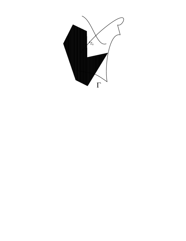
Figure 1: A typical position where Theorem 1.1 can be applied

Theorem 1.1

Let the support $\Gamma$ of a measure $\mu\in{\bf Reg}$ consist of finitely many continua, and let $z_{0}$ lie on the outer boundary of $\Gamma$. Assume that the intersection of $\Gamma$ with a neighborhood of $z_{0}$ is $C^{2}$-smooth arc $J$ which contains $z_{0}$ in its (one-dimensional) interior. Assume also that in this neighborhood $d\mu(z)=w(z)|z-z_{0}|^{\alpha}ds_{J}(z)$, where $w$ is a strictly positive continuous function and $\alpha>-1$. Then

$$\lim_{n\to\infty}n^{1+\alpha}\lambda_{n}(\mu,z_{0})=\frac{w(z_{0})}{(\pi\omega_{\Gamma}(z_{0}))^{\alpha+1}}2^{\alpha+1}\Gamma\Big{(}\frac{\alpha+1}{2}\Big{)}\Gamma\Big{(}\frac{\alpha+3}{2}\Big{)}.$$ (1.4)

The second main theorem of this work is about the behavior of the Christoffel function at an endpoint, see Figure 2. If $z_{0}$ is an endpoint of a smooth arc $J$ on the outer boundary of $\Gamma$, then at $z_{0}$ the equilibrium density has a $1/\sqrt{|z-z_{0}|}$ behavior (see the proof of Theorem 1.2), and we set

$$M(\Gamma,z_{0}):=\lim_{z\to z_{0},\ z\in\Gamma}\sqrt{|z-z_{0}|}\omega_{\Gamma}(z).$$ (1.5)

Theorem 1.2

Let $\Gamma$ and $\mu$ be as in Theorem 1.1, but now assume that the intersection of $\Gamma$ with a neighborhood of $z_{0}$ is $C^{2}$-smooth Jordan arc $J$ with one endpoint at $z_{0}$. Then

$$\lim_{n\to\infty}n^{2\alpha+2}\lambda_{n}(\mu,z_{0})=\frac{w(z_{0})}{(\pi M(\Gamma,z_{0}))^{2\alpha+2}}\Gamma(\alpha+1)\Gamma(\alpha+2).$$ (1.6)

These results can be used, in particular, if the measure is supported on a finite union of intervals on the real line, in which case the quantities $\omega_{\Gamma}(x)$ and $M(\Gamma,x)$ have a rather explicit form. Let $\Gamma=\cup_{j=0}^{k_{0}}[a_{2j},a_{2j+1}]$ with disjoint $[a_{2j},a_{2j+1}]$. Then the equilibrium density of $\Gamma$ is (see e.g. [23, (40), (41)] or [19, Lemma 4.4.1])

$$\omega_{\Gamma}(x)=\frac{\prod_{j=0}^{k_{0}-1}|x-\lambda_{j}|}{\pi\sqrt{\prod_{j=0}^{2k_{0}+1}|x-a_{j}|}},\qquad x\in{\rm Int}(\Gamma),$$ (1.7)

where $\lambda_{j}$ are the solutions of the system of equations

$$\int_{a_{2k+1}}^{a_{2k+2}}\frac{\prod_{j=0}^{k_{0}-1}(t-\lambda_{j})}{\sqrt{\prod_{j=0}^{2k_{0}+1}|t-a_{j}|}}dt=0,\qquad k=0,\ldots k_{0}-1.$$ (1.8)

It can be easily shown that these $\lambda_{j}$’s are uniquely determined and there is one $\lambda_{j}$ on every contiguous interval $(a_{2j+1},a_{2j+2})$. Now if $a$ is one of the endpoints of the intervals of $\Gamma$, say $a=a_{j_{0}}$, then

$$M(\Gamma,a)=\frac{\prod_{j=0}^{k_{0}-1}|a-\lambda_{j}|}{\pi\sqrt{\prod_{j=1,\ j\not=j_{0}}^{2k_{0}}|a-a_{j}|}}.$$ (1.9)

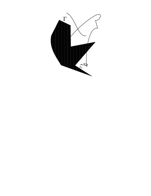
Figure 2: A typical position where Theorem 1.2 can be applied

This whole work is dedicated to proving Theorem 1.1 and Theorem 1.2. Actually, the latter will be a relatively easy consequence of the former one, so the main emphasis will be to prove Theorem 1.1. The main line of reasoning will be the following. We start from some known facts for simple measures like $|x|^{\alpha}dx$ on the real line, and get some elementary results for a model case on the unit circle via a transformation. Then we prove from these simple cases that Theorem 1.1 is true for lemniscate sets, i.e. level sets of polynomials. This part will use the polynomial mapping in question to transform the already known result to the given lemniscate. Then we prove the theorem for finite unions of Jordan curves. Recall that a Jordan curve is a homeomorhic image of a circle, while a Jordan arc is a homeomorhic image of a segment. From the point of view of finding the asymptotics of Christoffel functions there is a big difference between arcs and curves: Jordan curves have interior and can be exhausted by lemniscates, so the polynomial inverse image method of [23] is applicable for them, while for Jordan arc that method cannot be applied. Still, the pure Jordan curve case is used when we go over to a $\Gamma$ which may have arc components, namely it is used in the lower estimate. The upper estimate is the most difficult part of the proof; there Bessel functions enter the picture, and a discretization technique is developed where the discretization of the equilibrium measure of $\Gamma$ is done using the zeros of appropriate Bessel functions combined with another discretization based on uniform distribution. Once the case of Jordan curves and arcs have been settled, the proof of Theorem 1.1 will easily follow by approximating a general $\Gamma$ by a family of Jordan curves and arcs.

2 Tools

In what follows, $\|\cdot\|_{K}$ denotes the supremum norm on a set $K$, and $s_{\Gamma}$ the arc measure on $\Gamma$ (when $\Gamma$ consists of smooth Jordan arcs or curves).

We shall rely on some basic notions and facts from logarithmic potential theory. See the books [2], [3], [16] or [17] for detailed discussion.

We shall often use the trivial fact that if $\mu,\nu$ are two Borel measures, then $\mu\leq\nu$ implies $\lambda_{n}(\mu,x)\leq\lambda_{n}(\nu,x)$ for all $x$. It is also trivial that $\lambda_{n}(\mu,z)\leq\mu({\mathbb{C}})$ (just use the identically 1 polynomial as a test function in the definition of $\lambda_{n}(\mu,z)$).

Another frequently used fact is the following: if $\{n_{k}\}$ is a subsequence of the natural numbers such that $n_{k+1}/n_{k}\to 1$ as $k\to\infty$, then for any $\kappa>0$

$$\liminf_{n\to\infty}n^{\kappa}\lambda_{n}(\mu,x)=\liminf_{k\to\infty}n_{k}^{\kappa}\lambda_{n_{k}}(\mu,x),$$ (2.1)

and

$$\limsup_{n\to\infty}n^{\kappa}\lambda_{n}(\mu,x)=\limsup_{k\to\infty}n_{k}^{\kappa}\lambda_{n_{k}}(\mu,x).$$ (2.2)

In fact, since $\lambda_{n}(\mu,x)$ is a monotone decreasing function of $n$, for $n_{k}\leq n\leq n_{k+1}$ we have

$$\left(\frac{n}{n_{k+1}}\right)^{\kappa}n_{k+1}^{\kappa}\lambda_{n_{k+1}}(\mu,x)\leq n^{\kappa}\lambda_{n}(\mu,x)\leq\left(\frac{n}{n_{k}}\right)^{\kappa}n_{k}^{\kappa}\lambda_{n_{k}}(\mu,x),$$

and both claims follow because $n/n_{k}$ and $n/n_{k+1}$ tend to 1 as $n$ (or $n_{k}$) tends to infinity.

2.1 Fast decreasing polynomials

The following lemmas on the existence of fast decreasing polynomials will be a constant tool in the proofs.

Proposition 2.1

Let $K$ be a compact subset on $\mathbb{C}$, $\Omega$ the unbounded complement of $\mathbb{C}\setminus K$ and let $z_{0}\in\partial\Omega$. Suppose that there is a disk in $\Omega$ that contains $z_{0}$ on its boundary. Then, for every $\gamma>1$, there are constants $c_{\gamma},C_{\gamma}$, and for every $n\in\mathbb{N}$ polynomials $S_{n,z_{0},K}$ of degree at most $n$ such that $P_{n}(z_{0})=1$, $|S_{n,z_{0},K}(z)|\leq 1$ for all $z\in K$ and

$$|S_{n,z_{0},K}(z)|\leq C_{\gamma}e^{-nc_{\gamma}|z-z_{0}|^{\gamma}},\quad z\in K.$$ (2.3)

For details, see [22, Theorem 4.1]. This theorem will often be used in the following form.

Corollary 2.2

With the assumptions of Proposition 2.1 for every $0<\tau<1$, there exists constants $c_{\tau},C_{\tau},\tau_{0}>0$ and for every $n\in\mathbb{N}$ a polynomial $S_{n,z_{0},K}$ of degree $o(n)$ such that $S_{n,z_{0},K}(z_{0})=1$, $|S_{n,z_{0},K}(z)|\leq 1$ for all $z\in K$, and

$$|S_{n,z_{0},K}(z)|\leq C_{\tau}e^{-c_{\tau}n^{\tau_{0}}},\quad|z-z_{0}|\geq n^{-\tau}.$$ (2.4)

Proof.  Let $0<\varepsilon$ be sufficiently small and select $\gamma>1$ so that $1-\varepsilon-\tau\gamma>0$. Lemma 2.1 tells us that there is a polynomial $P_{n}$ with $\deg(P_{n})\leq n^{1-\varepsilon}$ such that

$$|P_{n}(z)|\leq C_{\gamma}e^{-c_{\gamma}n^{1-(\varepsilon+\tau\gamma)}},\quad|z-z_{0}|\geq n^{-\tau},$$

and this proves the claim with $S_{n,z_{0},K}=P_{n}$.  

There is a version of Lemma 2.1 where the decrease is not exponentially small, but starts much earlier than in Lemma 2.1.

Proposition 2.3

Let $K$ be as in Proposition 2.1. Then, for every $\beta<1$, there are constants $c_{\beta},C_{\beta}>0$, and for every $n=1,2,\ldots$ polynomials $P_{n}$ of degree at most $n$ such that $P_{n}(z_{0})=1$, $|P_{n}(z)|\leq 1$ for $z\in K$ and

$$|P_{n}(z)|\leq C_{\beta}e^{-c_{\beta}(n|z-z_{0}|)^{\beta}},\qquad z\in K.$$ (2.5)

See [25, Lemma 4].

It will be convenient to use these results when $n>1$ is not necessarily integer (formally one has to take the integral part of $n$, but the estimates will hold with possibly smaller constants in the exponents).

2.2 Polynomial inequalities

We shall also need some inequalities for polynomials that are used several times in the rest of the paper.

We start with a Bernstein-type inequality.

Lemma 2.4

Let $J$ be a $C^{2}$ closed Jordan arc and $J_{1}$ a closed subarc of $J$ not having common endpoint with $J$. Then, for every $D>0$, there is a constant $C_{D}$, such that

$$|P_{n}^{{}^{\prime}}(z)|\leq C_{D}n\|P_{n}\|_{J},\qquad\operatorname{dist}(z,J_{1})\leq D/n,$$

holds for any polynomials $P_{n}$ of degree $n=1,2,\ldots$.

See [22, Corollary 7.4].

Next, we continue with a Markov-type inequality.

Lemma 2.5

Let $K$ be a continuum. If $Q_{n}$ is a polynomial of degree at most $n=1,2,\ldots$, then

$$\|Q_{n}^{\prime}\|_{K}\leq\frac{e}{2{\rm cap}(K)}n^{2}\|Q_{n}\|_{K},$$ (2.6)

where ${\rm cap}(K)$ denotes the logarithmic capacity of $K$.

In particular, if $K$ has diameter 1, then

$$\|Q_{n}^{\prime}\|_{K}\leq 2en^{2}\|Q_{n}\|_{K}.$$ (2.7)

For (2.6) see [15, Theorem 1], and for the last statement note that if $K$ has diameter 1, then its capacity is at least $1/4$ ([16, Theorem 5.3.2(a)]).

Next, we prove a Remez-type inequality.

Lemma 2.6

Let $\Gamma$ be a $C^{1}$ Jordan curve or arc, and assume that for every $n=1,2,\ldots$, $J_{n}$ is a subarc of $\Gamma$, and $J_{n}^{*}$ is a subset of $J_{n}$ such that

$$s_{\Gamma}(J_{n}\setminus J_{n}^{*})=o(n^{-2})s_{\Gamma}(J_{n}),$$

where $s_{\Gamma}$ denotes the arc-length measure on $\Gamma$. Then, for any sequence $\{Q_{n}\}$of polynomials of degree at most $n=1,2,\ldots$, we have

$$\|Q_{n}\|_{J_{n}}=(1+o(1))\|Q_{n}\|_{J_{n}^{*}}.$$ (2.8)

Proof.  It is clear from the $C^{1}$ property that $s_{\Gamma}(J_{n})\sim{\rm diam}(J_{n})$ uniformly in $J_{n}$ (meaning that the ratio of the two sides lies in between two positive constants).

Make a linear transformation $z\to Cz$ such that, after this transformation, the arc $\tilde{J}_{n}$ that we obtain from $J_{n}$ has diameter 1. Under this transformation $J_{n}^{*}$ goes into a subset $\tilde{J}_{n}^{*}$ of $\tilde{J}_{n}$ for which

$$s_{\tilde{J}_{n}}(\tilde{J}_{n}\setminus\tilde{J}_{n}^{*})=o(n^{-2})s_{\tilde{J}_{n}}(\tilde{J}_{n}),$$ (2.9)

and $Q_{n}$ changes into a polynomial $\tilde{Q}_{n}$ of degree at most $n$. (2.8) is clearly equivalent to its $\tilde{}$-version.

Let $M=\|\tilde{Q}_{n}\|_{\tilde{J}_{n}}$. By Lemma 2.5, the absolute value of $\tilde{Q}_{n}^{\prime}$ is bounded on $\tilde{J}_{n}$ by $2en^{2}M$, hence if $z,w\in\tilde{J}_{n}$, then

$$|\tilde{Q}_{n}(z)-\tilde{Q}_{n}(w)|\leq 2en^{2}Ms_{\tilde{J}_{n}}(\overline{zw}),$$ (2.10)

where $\overline{zw}$ is the arc of $\tilde{J}_{n}$ lying in between $z$ and $w$. By the assumption (2.9) for every $z\in\tilde{J}_{n}$ there is a $w\in\tilde{J}_{n}^{*}$ with

$$s_{\tilde{J}_{n}}(\overline{zw})=o(n^{-2})s_{\tilde{J}_{n}}(\tilde{J}_{n})=o(n^{-2})$$

because $s_{\tilde{J}_{n}}(\tilde{J}_{n})\sim{\rm diam}(\tilde{J}_{n})=1$. Choose here $z\in\tilde{J}_{n}$ such that $|\tilde{Q}_{n}(z)|=M$. Since $|\tilde{Q}_{n}(w)|\leq\|\tilde{Q}_{n}\|_{\tilde{J}_{n}^{*}}$, we get from (2.10)

$$M=|\tilde{Q}_{n}(z)|\leq\|\tilde{Q}_{n}\|_{\tilde{J}_{n}^{*}}+o(1)M,$$

and the claim follows.  

We shall frequently use the following, so called Nikolskii-type inequalities for power type weights. In it we write that a Jordan arc is $C^{1+}$-smooth if there is a $\theta>0$ such that the arc in question is $C^{1+\theta}$-smooth.

Lemma 2.7

Let $J$ be a $C^{1+}$-smooth Jordan arc and let $J^{*}\subset J$ be a subarc of $J$ which has no common endpoint with $J$. Let $z_{0}\in J$ be a fixed point, and for $\alpha>-1$ define the measure $\nu_{\alpha}$ on $J$ by $d\nu_{\alpha}(u)=|u-z_{0}|^{\alpha}ds_{J}(u)$. Then there is a constant $C$ depending only on $\alpha,J$ and $J^{*}$ such that for any polynomials $P_{n}$ of degree at most $n=1,2,\ldots$ we have

$$\|P_{n}\|_{J^{*}}\leq Cn^{(1+\alpha)/2}\|P_{n}\|_{L^{2}(\nu_{\alpha})},$$ (2.11)

if $\alpha\geq 0$, and

$$\|P_{n}\|_{J^{*}}\leq Cn^{1/2}\|P_{n}\|_{L^{2}(\nu_{\alpha})},$$ (2.12)

if $-1<\alpha<0$.

The same is true if $d\nu_{\alpha}(u)=w(u)|u-z_{0}|^{\alpha}ds_{J}(u)$ with some strictly positive and continuous $w$.

Proof.  In view of [26, Lemmas 3.8 and Corollary 3.9] (use also that $\nu_{\alpha}$ is a doubling weight in the sense of [26]) uniformly in $z\in J^{*}$ we have for large $n$ the relation

$$\lambda_{n}(\nu_{\alpha},z)\sim\nu_{\alpha}(l_{1/n}(z)),$$

where $A\sim B$ means that the ratio lies in between two constants, and where $l_{1/n}(z)$ is the arc of $J$ consisting of those points of $z$ that lie of distance $\leq 1/n$ from $z$. If $\alpha\geq 0$, then

$$\nu_{\alpha}(l_{1/n}(z))\geq\frac{c}{n^{1+\alpha}},$$

while for $-1<\alpha<0$

$$\nu_{\alpha}(l_{1/n}(z))\geq\frac{c}{n},$$

with some positive constant $c$ which depends only on $\alpha,J$ and $J^{*}$. Therefore, we have for all $z\in J^{*}$ the inequality

$$\lambda_{n}(\nu_{\alpha},z)\geq\frac{c}{n^{1+\alpha}}$$ (2.13)

if $\alpha\geq 0$ and

$$\lambda_{n}(\nu_{\alpha},z)\geq\frac{c}{n}$$ (2.14)

when $-1<\alpha<0$.

For example, (2.13) means that if $\alpha\geq 0$ and $|P_{n}(z)|=1$ for some $z\in J^{*}$, then necessarily

$$\frac{n^{1+\alpha}}{c}\int_{J}|P_{n}|^{2}d\nu_{\alpha}\geq 1,$$

which is equivalent to saying that for any $P_{n}$ and $z\in J^{*}$

$$\frac{n^{1+\alpha}}{c}\int_{J}|P_{n}|^{2}d\nu_{\alpha}\geq|P_{n}(z)|^{2},$$

and this is (2.11). In a similar manner, (2.12) follows from (2.14).

It is clear that this proof does not change if $\nu_{\alpha}$ is as in the last sentence of the lemma.  

Lemma 2.8

If $\alpha>-1$, then there is a constant $C_{\alpha}$ such that for any polynomial $P_{n}$ of degree at most $n$ the inequality

$$\|P_{n}\|_{[-1,1]}\leq C_{\alpha}n^{(1+\alpha^{*})/2}\left(\int_{-1}^{1}|P_{n}(x)|^{2}|x|^{\alpha}dx\right)^{1/2}$$ (2.15)

holds with $\alpha^{*}=\max(1,\alpha)$.

Proof.  We follow the preceding proof, but now both $J$ and $J^{*}$ agree with $[-1,1]$.

Let $J=J^{*}=[-1,1]$, $z_{0}=0$, $\Delta_{n}(z)=1/n^{2}$ if $z\in[-1,-1+1/n^{2}]$ or $z\in[1-1/n^{2},1]$, and set $\Delta_{n}(z)=\sqrt{1-z^{2}}/n$ if $z\in[-1+1/n^{2},1-1/n^{2}]$. If now $l_{1/n}(z)$ is the interval $[z-\Delta_{n}(z),z+\Delta_{n}(z)]$ intersected with $[-1,1]$, then [26, Lemmas 3.8 and Corollary 3.9] state that for $d\nu_{\alpha}(x)=|x-z_{0}|^{\alpha}dx=|x|^{\alpha}dx$ on $[-1,1]$ we have

$$\lambda_{n}(\nu_{\alpha},z)\sim\nu_{\alpha}(l_{1/n}(z)).$$

If $\alpha\geq 0$, then

$$\nu_{\alpha}(l_{1/n}(z))\geq c\min\left(\frac{1}{n^{2}},\frac{1}{n^{1+\alpha}}\right),$$

while for $-1<\alpha<0$

$$\nu_{\alpha}(l_{1/n}(z))\geq\frac{c}{n^{2}},$$

with some positive constant $c$. Hence,

$$\lambda_{n}(\nu_{\alpha},z)\geq\frac{c}{n^{2}}$$

if $-1<\alpha\leq 1$, while

$$\lambda_{n}(\nu_{\alpha},z)\geq\frac{c}{n^{1+\alpha}}$$

if $\alpha\geq 1$, from which (2.15) follows exactly as before.  

The Nikolskii inequalties can be combined with the following estimate to get an upper bound for the extremal polynomials that produce $\lambda_{n}(\mu,z)$.

Lemma 2.9

With the assumptions of Theorem 1.1 we have

$$\lambda_{n}(\mu,z_{0})\leq Cn^{-(\alpha+1)}$$

with some constant $C$ that is independent of $n$.

Proof.  Just use the polynomials $S_{n,z_{0},\Gamma}$ from Proposition 2.3 with $\beta=1/2$ and $K=\Gamma$. Let $\delta>0$ be so small that in the $\delta$-neighborhood of $z_{0}$ we have the $d\mu(z)=w(z)|z-z_{0}|^{\alpha}ds_{\Gamma}(z)$ representation for $\mu$. Outside this $\delta$-neighborhood $|S_{n,z_{0},\Gamma}|$ is smaller than $C_{\beta}\exp(-c_{\beta}(n\delta)^{1/2})$, so

$$\int|S_{n,z_{0},\Gamma}|^{2}d\mu\leq C\int e^{-2c_{\beta}(n|t|)^{1/2}}|t|^{\alpha}dt+Ce^{-2c_{\beta}(n\delta)^{1/2}}\leq Cn^{-\alpha-1},$$

which proves the claim.  

We close this section with the classical Bernstein-Walsh lemma, see [27, p. 77].

Lemma 2.10

Let $K\subset{\mathbb{C}}$ be a compact subset of positive logarithmic capacity, let $\Omega$ be the unbounded component of $\overline{\mathbb{C}}\setminus K$, and $g_{\Omega}$ the Green’s function of this unbounded component with pole at infinity. Then, for polynomials $P_{n}$ of degree at most $n=1,2,\ldots$, we have for any $z\in{\mathbb{C}}$

$$|P_{n}(z)|\leq e^{ng_{\Omega}(z)}\|P_{n}\|_{K}.$$

3 The model cases

3.1 Measures on the real line

Our first goal is to establish asymptotics for the Christoffel function at $0$ with respect to the measure $d\mu(x)=|x|^{\alpha}dx$, $x\in[-1,1]$. We do this by transforming some previously known results.

In what follows, for simpler notations, if $d\mu(x)=w(x)dx$, then we shall write $\lambda_{n}(w(x),z)$ for $\lambda_{n}(\mu,z)$.

Proposition 3.1

For $\alpha>-1$ we have

$$\lim_{n\to\infty}n^{2\alpha+2}\lambda_{n}\left({|x|^{\alpha}\,\vrule\,\lower 7.5347pt\hbox{{\scriptsize$[0,1]$}}},0\right)=\Gamma(\alpha+1)\Gamma(\alpha+2).$$ (3.1)

Proof.  It follows from [10, (1.10)] or [9, Theorem 4.1] that

$$\lim_{n\to\infty}n^{2\alpha+2}\lambda_{n}\left({(1-x)^{\alpha}\,\vrule\,\lower 7.5347pt\hbox{{\scriptsize$[-1,1]$}}},1\right)=2^{\alpha+1}\Gamma(\alpha+1)\Gamma(\alpha+2),$$ (3.2)

from which the claim is an immediate consequence if we apply the linear transformation $x\to(1-x)/2$.  

Proposition 3.2

For $\alpha>-1$ we have

$$\lim_{n\to\infty}n^{\alpha+1}\lambda_{n}\left({|x|^{\alpha}\,\vrule\,\lower 7.5347pt\hbox{{\scriptsize$[-1,1]$}}},0\right)=L_{\alpha},$$ (3.3)

where

$$L_{\alpha}:=2^{\alpha+1}\Gamma\Big{(}\frac{\alpha+1}{2}\Big{)}\Gamma\Big{(}\frac{\alpha+3}{2}\Big{)}.$$ (3.4)

Proof.  Let us agree that in this proof, whenever we write $P_{n},R_{n}$ etc. for polynomials, then it is understood that the degree is at most $n$.

We use that (for continuous $f$)

$$\int_{0}^{1}f(x)|x|^{\alpha}dx=\int_{-1}^{1}f(x^{2})|x|^{2\alpha+1}dx.$$ (3.5)

Assume first that $P_{2n}$ is extremal for $\lambda_{2n}\left({|x|^{\alpha}\,\vrule\,\lower 7.5347pt\hbox{{\scriptsize$[-1,1]$}}},0\right)$, i.e. $P_{2n}(0)=1$ and

$$\int_{-1}^{1}|P_{2n}(x)|^{2}|x|^{\alpha}dx=\lambda_{2n}\left({|x|^{\alpha}\,\vrule\,\lower 7.5347pt\hbox{{\scriptsize$[-1,1]$}}},0\right).$$

Define

$$R_{n}(x)=\frac{P_{2n}(x)+P_{2n}(-x)}{2}.$$

Then $R_{n}(0)=1$, and $R_{n}$ is a polynomial in $x^{2}$, hence $R_{n}(x)=R_{n}^{*}(x^{2})$ with some polynomial $R_{n}^{*}$, for which $R_{n}^{*}(0)=1$ and $\deg(R_{n}^{*})\leq n$. Now we have

$$\int_{-1}^{1}|R_{n}(x)|^{2}|x|^{\alpha}dx=\int_{-1}^{1}|R_{n}^{*}(x^{2})|^{2}|x|^{\alpha}dx = \int_{0}^{1}|R_{n}^{*}(x)|^{2}|x|^{\frac{\alpha-1}{2}}dx$$

$$\geq \lambda_{n}\left({|x|^{\frac{\alpha-1}{2}}\,\vrule\,\lower 7.5347pt\hbox{{\scriptsize$[0,1]$}}},0\right).$$

With the Cauchy-Schwarz inequality and with the symmetry of the measure $|x|^{\alpha}dx$, we have

$$\int_{-1}^{1}|R_{n}(x)|^{2}|x|^{\alpha}dx \leq\frac{1}{4}\int_{-1}^{1}\Big{(}|P_{2n}(x)|^{2}+2|P_{2n}(x)||P_{2n}(-x)|+|P_{2n}(-x)|^{2}\Big{)}|x|^{\alpha}dx$$

$$\leq\frac{1}{2}\int_{-1}^{1}|P_{2n}(x)|^{2}|x|^{\alpha}dx$$

$$+\frac{1}{2}\Bigg{(}\int_{-1}^{1}|P_{2n}(x)|^{2}|x|^{\alpha}dx\Bigg{)}^{1/2}\Bigg{(}\int_{-1}^{1}|P_{2n}(-x)|^{2}|x|^{\alpha}dx\Bigg{)}^{1/2}$$

$$=\int_{-1}^{1}|P_{2n}(x)|^{2}|x|^{\alpha}dx=\lambda_{2n}\left({|x|^{\alpha}\,\vrule\,\lower 7.5347pt\hbox{{\scriptsize$[-1,1]$}}},0\right).$$

Combining these two estimates, we obtain

$$\lambda_{n}\left({|x|^{\frac{\alpha-1}{2}}\,\vrule\,\lower 7.5347pt\hbox{{\scriptsize$[0,1]$}}},0\right)\leq\lambda_{2n}\left({|x|^{\alpha}\,\vrule\,\lower 7.5347pt\hbox{{\scriptsize$[-1,1]$}}},0\right).$$

On the other hand, if now $P_{n}$ is extremal for $\lambda_{n}\left({|x|^{\frac{\alpha-1}{2}}\,\vrule\,\lower 7.5347pt\hbox{{\scriptsize$[0,1]$}}},0\right)$, then

$$\lambda_{n}\left({|x|^{\frac{\alpha-1}{2}}\,\vrule\,\lower 7.5347pt\hbox{{\scriptsize$[0,1]$}}},0\right)=\int_{0}^{1}|P_{n}(x)|^{2}|x|^{\frac{\alpha-1}{2}}dx = \int_{-1}^{1}|P_{n}(x^{2})|^{2}|x|^{\alpha}dx$$

$$\geq \lambda_{2n}\left({|x|^{\alpha}\,\vrule\,\lower 7.5347pt\hbox{{\scriptsize$[-1,1]$}}},0\right),$$

therefore we actually have the equality

$$\lambda_{n}\left({|x|^{\frac{\alpha-1}{2}}\,\vrule\,\lower 7.5347pt\hbox{{\scriptsize$[0,1]$}}},0\right)=\lambda_{2n}\left({|x|^{\alpha}\,\vrule\,\lower 7.5347pt\hbox{{\scriptsize$[-1,1]$}}},0\right),$$ (3.6)

from which the claim follows via Proposition 3.1 (see also (2.1) and (2.2) with $n_{k}=2k$).

Note also that this proves also that if $P_{n}(x)$ is the $n$-degree extremal polynomials for the measure ${|x|^{\frac{\alpha-1}{2}}\,\vrule\,\lower 7.5347pt\hbox{{\scriptsize$[0,1]$}}}$, then $P_{n}(x^{2})$ is the $2n$-degree extremal polynomial for the measure ${|x|^{\alpha}\,\vrule\,\lower 7.5347pt\hbox{{\scriptsize$[-1,1]$}}}$.

 

3.2 Measures on the unit circle

Let $\mu_{\mathbb{T}}$ be the measure on the unit circle $\mathbb{T}$ defined by $d\mu_{\mathbb{T}}(e^{it})=w_{\mathbb{T}}(e^{it})dt$, where

$$w_{\mathbb{T}}(e^{it})=\frac{|e^{2it}+1|^{\alpha}}{2^{\alpha}}\frac{|e^{2it}-1|}{2},\qquad t\in[-\pi,\pi).$$ (3.7)

We shall prove

$$\lim_{n\to\infty}n^{\alpha+1}\lambda_{n}(\mu_{\mathbb{T}},e^{i\pi/2})=2^{\alpha+1}L_{\alpha}$$ (3.8)

where $L_{\alpha}$ is from (3.4), by transforming the measure $\mu_{\mathbb{T}}$ into a measure $\mu_{[-1,1]}$ supported on the interval $[-1,1]$ and comparing the Christoffel functions for them. With the transformation $e^{it}\to\cos t$, we have

$$\int_{-\pi}^{\pi}f(\cos t)w_{\mathbb{T}}(e^{it})dt=2\int_{-1}^{1}f(x)w_{[-1,1]}(x)dx,$$

where

$$w_{[-1,1]}(x)=|x|^{\alpha}.$$

Set $d\mu_{[-1,1]}(x)=w_{[-1,1]}(x)dx$.

Let $P_{n}$ be the extremal polynomial for $\lambda_{n}(\mu_{[-1,1]},0)$ and define

$$S_{n}(e^{it})=P_{n}(\cos t)\Bigg{(}\frac{1+e^{i(t-\pi/2)}}{2}\Bigg{)}^{\lfloor\eta n\rfloor}e^{in(t-\pi/2)},$$

where $\eta>0$ is arbitrary. This $S_{n}$ is a polynomial of degree $2n+\lfloor\eta n\rfloor$ with $S_{n}(e^{i\pi/2})=1$. For any fixed $0<\delta<1$

$$\int_{\pi/2-\delta}^{\pi/2+\delta}|S_{n}(e^{it})|^{2}w_{\mathbb{T}}(e^{it})dt \leq\int_{\pi/2-\delta}^{\pi/2+\delta}|P_{n}(\cos t)|^{2}w_{\mathbb{T}}(e^{it})dt$$ (3.9)

$$\leq\int_{-1}^{1}|P_{n}(x)|^{2}w_{[-1,1]}(x)dx$$

$$=\lambda_{n}(\mu_{[-1,1]},0).$$

To estimate the corresponding integral over the intervals $[-\pi,\pi/2-\delta]$ and $[\pi/2+\delta,\pi]$, notice that

$$\max_{t\in[-\pi,\pi]\setminus[\pi/2-\delta,\pi/2+\delta]}\Bigg{|}\frac{1+e^{i(t-\pi/2)}}{2}\Bigg{|}^{\lfloor\eta n\rfloor}=O(q^{n})$$ (3.10)

for some $q<1$. From Lemma 2.8 we obtain

$$\|P_{n}\|_{[-1,1]}\leq Cn^{{1+|\alpha|}/2}\|P_{n}\|_{L^{2}(\mu_{[-1,1]})}\leq Cn^{1+|\alpha|/2},$$

and so

$$\left(\int_{-\pi}^{\pi/2-\delta}+\int_{\pi/2+\delta}^{\pi}\right)|S_{n}(e^{it})|^{2}w_{\mathbb{T}}(e^{it})dt=O(n^{1+|\alpha|/2}q^{n})=o(n^{-\alpha-1}).$$

Therefore, using this $S_{n}$ as a test polynomial for $\lambda_{\deg(S_{n})}(\mu_{\mathbb{T}},e^{i\pi/2})$ we conclude

$$\lambda_{\deg(S_{n})}(\mu_{\mathbb{T}},e^{i\pi/2})\leq\lambda_{n}(\mu_{[-1,1]},0)+o(n^{-\alpha-1}),$$

and so

$$\limsup_{n\to\infty}\big{(}2n+\lfloor\eta n\rfloor\big{)}^{\alpha+1}\lambda_{2n+\lfloor\eta n\rfloor}(\mu_{\mathbb{T}},e^{i\pi/2}) \leq\limsup_{n\to\infty}\big{(}2+\lfloor\eta n\rfloor/n\big{)}^{\alpha+1}n^{\alpha+1}\lambda_{n}(\mu_{[-1,1]},0)$$

$$=(2+\eta)^{\alpha+1}L_{\alpha},$$

where we used Proposition 3.2 for the measure $\mu_{[-1,1]}$.

Since $\eta>0$ was arbitrary,

$$\limsup_{n\to\infty}n^{\alpha+1}\lambda_{n}(\mu_{\mathbb{T}},e^{i\pi/2})\leq 2^{\alpha+1}L_{\alpha}$$ (3.11)

follows (see also (2.2)).

Now to prove the matching lower estimate, let $S_{2n}(e^{it})$ be the extremal polynomial for $\lambda_{2n}(\mu_{\mathbb{T}},e^{i\pi/2})$. Define

$$P_{n}^{*}(e^{it})=S_{2n}(e^{it})\Bigg{(}\frac{1+e^{i(t-\pi/2)}}{2}\Bigg{)}^{2\lfloor\eta n\rfloor}e^{-(n+\lfloor\eta n\rfloor)i(t-\pi/2)}$$

and $P_{n}(\cos t)=P_{n}^{*}(e^{it})+P_{n}^{*}(e^{-it})$. Note that $P_{n}(\cos t)$ is a polynomial in $\cos t$ of $\deg(P_{n})\leq n+\lfloor\eta n\rfloor$ and $P_{n}(0)=1$. With it we have

$$\lambda_{\deg(P_{n})}(\mu_{[-1,1]},0)\leq\int_{-1}^{1}|P_{n}(x)|^{2}w_{[-1,1]}(x)dx=\frac{1}{2}\int_{-\pi}^{\pi}|P_{n}(\cos t)|^{2}w_{\mathbb{T}}(e^{it})dt.$$ (3.12)

First, we claim that for every fixed $0<\delta<1$

$$|P_{n}(\cos t)|^{2} =|P_{n}^{*}(e^{it})|^{2}+O(q^{n}),\quad t\in[\pi/2-\delta,\pi/2+\delta],$$ (3.13)

$$|P_{n}(\cos t)|^{2} =|P_{n}^{*}(e^{-it})|^{2}+O(q^{n}),\quad t\in[-\pi/2-\delta,-\pi/2+\delta],$$

$$|P_{n}(\cos t)|^{2} =O(q^{n})\quad\textnormal{otherwise,}$$

hold for some $q<1$. Indeed,

$$|P_{n}(\cos t)|^{2}=|P_{n}^{*}(e^{it})+P_{n}^{*}(e^{-it})|^{2}\leq|P_{n}^{*}(e^{it})|^{2}+2|P_{n}^{*}(e^{it})||P_{n}^{*}(e^{-it})|+|P_{n}^{*}(e^{-it})|^{2}.$$

If we apply Lemma 2.7 to two subarcs (say of length $5\pi/4$) of $\mathbb{T}$ that contain the upper, resp. the lower half of the unit circle, then we obtain that

$$\|P_{n}^{*}\|_{\mathbb{T}}\leq\|S_{2n}\|_{\mathbb{T}}\leq Cn^{(1+|\alpha|)/2}\|S_{2n}\|_{L^{2}(\mu_{\mathbb{T}})}\leq Cn^{(1+|\alpha|)/2}.$$

Therefore (use (3.10))

$$|P_{n}^{*}(e^{it})|\leq Cq^{n}n^{(1+|\alpha|)/2},\quad t\in[-\pi,\pi]\setminus[\pi/2-\delta,\pi/2+\delta].$$

These imply (3.13).

Now we have

$$\int_{-\pi}^{\pi}|P_{n}(\cos t)|^{2}w_{\mathbb{T}}(e^{it})dt =\Bigg{(}\int_{\pi/2-\delta}^{\pi/2+\delta}+\int_{-\pi/2-\delta}^{-\pi/2+\delta}\Bigg{)}|P_{n}(\cos t)|^{2}w_{\mathbb{T}}(e^{it})dt$$

$$+\Bigg{(}\int_{-\pi}^{-\pi/2-\delta}+\int_{-\pi/2+\delta}^{\pi/2-\delta}+\int_{\pi/2+\delta}^{\pi}\Bigg{)}|P_{n}(\cos t)|^{2}w_{\mathbb{T}}(e^{it})dt.$$

(3.13) tells us that the last three terms are $O(q^{n})$. For the other two terms we have, again by (3.13),

$$\int_{\pi/2-\delta}^{\pi/2+\delta}|P_{n}(\cos t)|^{2}w_{\mathbb{T}}(e^{it})dt =\int_{\pi/2-\delta}^{\pi/2+\delta}|P_{n}^{*}(e^{it})|^{2}w_{\mathbb{T}}(e^{it})dt+O(q^{n})$$

$$\leq\int_{\pi/2-\delta}^{\pi/2+\delta}|S_{2n}(e^{it})|^{2}w_{\mathbb{T}}(e^{it})dt+O(q^{n})$$

$$\leq\lambda_{2n}(\mu_{\mathbb{T}},e^{i\pi/2})+O(q^{n})$$

and similarly,

$$\int_{-\pi/2-\delta}^{-\pi/2+\delta}|P_{n}(\cos t)|^{2}w_{\mathbb{T}}(e^{it})dt\leq\lambda_{2n}(\mu_{\mathbb{T}},e^{i\pi/2})+O(q^{n}).$$

Combining these estimates with (3.12), we can conclude

$$\lambda_{\deg(P_{n})}(\mu_{[-1,1]},0)\leq\lambda_{2n}(\mu_{\mathbb{T}},e^{i\pi/2})+O(q^{n}),$$

therefore

$$\liminf_{n\to\infty}\deg(P_{n})^{\alpha+1} \lambda_{\deg(P_{n})}(\mu_{[-1,1]},0)\leq\liminf_{n\to\infty}(n+\lfloor\eta n\rfloor)^{\alpha+1}\big{(}\lambda_{2n}(\mu_{\mathbb{T}},e^{i\pi/2})+O(q^{n})\big{)}$$

$$\leq\liminf_{n\to\infty}(1+\lfloor\eta n\rfloor/n)^{\alpha+1}\frac{1}{2^{\alpha+1}}(2n)^{\alpha+1}\lambda_{2n}(\mu_{\mathbb{T}},e^{i\pi/2}).$$

From this, in view of Proposition 3.2 and (2.1), it follows that

$$(1+\eta)^{-(\alpha+1)}2^{\alpha+1}L_{\alpha}\leq\liminf_{n\to\infty}\lambda_{n}(\mu_{\mathbb{T}},e^{i\pi/2}),$$

and upon letting $\eta\to 0$ we obtain

$$2^{\alpha+1}L_{\alpha}\leq\liminf_{n\to\infty}\lambda_{n}(\mu_{\mathbb{T}},e^{i\pi/2}).$$ (3.14)

This and (3.11) verify (3.8).

Finally, let

$$d\mu_{\alpha}(e^{it})=|e^{it}-i|^{\alpha}dt.$$

Let us write $|e^{it}-i|^{\alpha}$ in the form

$$|e^{it}-i|^{\alpha}=w(e^{it})w_{\mathbb{T}}(e^{it}).$$

Then $w$ is continuous in a neighborhood of $e^{i\pi/2}$ and it has value 1 at $e^{i\pi/2}$. Let $\tau>0$ be arbitrary, and choose $0<\delta<1$ in such a way that

$$\frac{1}{1+\tau}\leq w(e^{it})\leq(1+\tau),\qquad t\in[\pi/2-\delta,\pi/2+\delta].$$

If we now carry out the preceding arguments with this $\delta$ and with this $\mu_{\alpha}$ replacing everywhere $\mu_{\mathbb{T}}$, then we get that in (3.11) the limsup is at most $(1+\tau)2^{\alpha+1}L_{\alpha}$, while in (3.14) the liminf is at least $(1+\tau)^{-1}2^{\alpha+1}L_{\alpha}$. Since $\tau>0$ can be arbitrarily chosen, this shows that

$$\lim_{n\to\infty}n^{\alpha+1}\lambda_{n}(\mu_{\alpha},e^{i\pi/2})=2^{\alpha+1}L_{\alpha}.$$ (3.15)

This result will serve as our model case in the proof of Theorem 1.1.

4 Lemniscates

In this section, we prove Theorem 1.1 for lemniscates.

Let $\sigma=\{z\in\mathbb{C}:|T_{N}(z)|=1\}$ be the level line of a polynomial $T_{N}$, and assume that $\sigma$ has no self-intersections. Let $\deg(T_{N})=N$.

The normal derivative of the Green’s function with pole at infinity of the outer domain to $\sigma$ at a point $z\in\sigma$ is (see [22, (2.2)]) $|T_{N}^{\prime}(z)|/N$, and since this normal derivative is $2\pi$-times the equilibrium density of $\sigma$ (see [14, II.(4.1)] or [17, Theorem IV.2.3] and [17, (I.4.8)]), it follows that the equilibrium density on $\sigma$ has the form

$$\omega_{\sigma}(z)=\frac{|T_{N}^{\prime}(z)|}{2\pi N}.$$ (4.1)

If $z\in\sigma$, then there are $n$ points $z_{1},\ldots,z_{n}\in\sigma$ with the property $T_{N}(z)=T_{n}(z_{k})$, and for them (see [22, (2.12)])

$$\int_{\sigma}\Big{(}\sum_{i=1}^{N}f(z_{i})\Big{)}|T_{N}^{{}^{\prime}}(z)|ds_{\sigma}(z)=N\int_{\sigma}f(z)|T_{N}^{{}^{\prime}}(z)|ds_{\sigma}(z).$$ (4.2)

Furthermore, if $g:\mathbb{T}\to\mathbb{C}$ is arbitrary, then (see [22, (2.14)])

$$\int_{\sigma}g(T_{N}(z))|T_{N}^{{}^{\prime}}(z)|ds_{\sigma}(z)=N\int_{0}^{2\pi}g(e^{it})dt.$$ (4.3)

Let $z_{0}\in\sigma$ be arbitrary, and define the measure

$$d\mu_{\sigma}(z)=|z-z_{0}|^{\alpha}ds_{\sigma}(z),\quad\alpha>-1,$$ (4.4)

where $s_{\sigma}$ denotes the arc measure on $\sigma$. Without loss of generality we may assume that $T_{N}(z_{0})=e^{i\pi/2}$. Our plan is to compare the Chritoffel functions for the measure $\mu_{\sigma}$ with that for the measure $\mu_{\alpha}$ which is supported on the unit circle and is defined via

$$d\mu_{\alpha}(e^{it})=|e^{it}-e^{i\pi/2}|^{\alpha}ds_{\mathbb{T}}(e^{it}),$$ (4.5)

and for which the asymptotics of the Christoffel function was calculated in (3.15).

We shall prove that

$$\lim_{n\to\infty}n^{\alpha+1}\lambda_{n}(\mu_{\sigma},z_{0})=\frac{L_{\alpha}}{(\pi\omega_{\sigma}(z_{0}))^{\alpha+1}}$$ (4.6)

where $L_{\alpha}$ is taken from (3.4).

4.1 The upper estimate

Let $\eta>0$ be an arbitrary small number, and select a $\delta>0$ such that for every $z$ with $|z-z_{0}|<\delta$, we have

$$\frac{1}{1+\eta}|T_{N}^{{}^{\prime}}(z_{0})| \leq|T_{N}^{{}^{\prime}}(z)|\leq(1+\eta)|T_{N}^{{}^{\prime}}(z_{0})|$$ (4.7)

$$\frac{1}{1+\eta}|T_{N}^{{}^{\prime}}(z_{0})||z-z_{0}| \leq|T_{N}(z)-T_{N}(z_{0})|\leq(1+\eta)|T_{N}^{{}^{\prime}}(z_{0})||z-z_{0}|$$

(note that $T_{N}^{\prime}(z_{0})\not=0$ because $\sigma$ has no self-intersections). Let $Q_{n}$ be the extremal polynomial for $\lambda_{n}(\mu_{\alpha},e^{i\pi/2})$, where $\mu_{\alpha}$ is from (4.5). Define $R_{n}$ as

$$R_{n}(z)=Q_{n}(T_{N}(z))S_{n,z_{0},L}(z),$$

where $S_{n,z_{0},L}$ is the fast decreasing polynomial given by Corollary 2.2 for the lemniscate set $L$ enclosed by $\sigma$ (and for any fixed $0<\tau<1$ in Corollary 2.2). Note that $R_{n}$ is a polynomial of degree $nN+o(n)$ with $R_{n}(z_{0})=1$. Since $S_{n,z_{0},L}$ is fast decreasing, we have

$$\sup_{z\in L\setminus\{z:|z-z_{0}|<\delta\}}|S_{n,z_{0},L}(z)|=O(q^{n^{\tau_{0}}})$$

for some $q<1$ and $\tau_{0}>0$. The Nikolskii-type inequality in Lemma 2.7 when applied to two subarcs of $\mathbb{T}$ which contain the upper resp. lower part of the unit circle, yields

$$\|Q_{n}\|_{\mathbb{T}}\leq Cn^{(1+|\alpha|)/2}\|Q_{n}\|_{L^{2}(\mu_{\alpha})}\leq Cn^{(1+|\alpha|)/2}.$$

Therefore,

$$\sup_{z\in L\setminus\{z:|z-z_{0}|<\delta\}}|R_{n}(z)|=O(q^{n^{\tau_{0}/2}}).$$

It follows that

$$\int_{|z-z_{0}|\geq\delta}|R_{n}(z)|^{2}|z-z_{0}|^{\alpha}ds_{\sigma}(z)=O(q^{n^{\tau_{0}/2}}).$$ (4.8)

Using (4.7), we have

$$\int_{|z-z_{0}|<\delta}|R_{n}(z)|^{2} |z-z_{0}|^{\alpha}ds_{\sigma}(z)$$

$$\leq\int_{|z-z_{0}|<\delta}|Q_{n}(T_{N}(z))|^{2}|z-z_{0}|^{\alpha}ds_{\sigma}(z)$$

$$\leq\frac{(1+\eta)^{|\alpha|+1}}{|T_{N}^{{}^{\prime}}(z_{0})|^{\alpha+1}}\int_{|z-z_{0}|<\delta}|Q_{n}(T_{N}(z))|^{2}|T_{N}(z)-T_{N}(z_{0})|^{\alpha}|T_{N}^{{}^{\prime}}(z)|ds_{\sigma}(z)$$

$$\leq\frac{(1+\eta)^{|\alpha|+1}}{|T_{N}^{{}^{\prime}}(z_{0})|^{\alpha+1}}\int_{0}^{2\pi}|Q_{n}(e^{it})|^{2}|e^{it}-e^{i\pi/2}|^{\alpha}dt$$

$$=(1+\eta)^{|\alpha|+1}\frac{\lambda_{n}(\mu_{\alpha},e^{i\pi/2})}{|T_{N}^{{}^{\prime}}(z_{0})|^{\alpha+1}}.$$

This and (4.8) imply

$$\lambda_{\deg(R_{n})}(\mu_{\sigma},z_{0})\leq(1+\eta)^{|\alpha|+1}\frac{\lambda_{n}(\mu_{\alpha},e^{i\pi/2})}{|T_{N}^{{}^{\prime}}(e^{i\pi/2})|^{\alpha+1}}+O(q^{n^{\tau_{0}/2}}),$$

from which

$$\limsup_{n\to\infty}\deg(R_{n})^{\alpha+1} \lambda_{\deg(R_{n})}(\mu_{\sigma},z_{0})$$

$$\leq\limsup_{n\to\infty}(nN+o(n))^{\alpha+1}(1+\eta)^{|\alpha|+1}\frac{\lambda_{n}(\mu_{\alpha},e^{i\pi/2})}{|T_{N}^{{}^{\prime}}(z_{0})|^{\alpha+1}}$$

$$=(1+\eta)^{|\alpha|+1}\frac{N^{\alpha+1}}{|T_{N}^{{}^{\prime}}(z_{0})|^{\alpha+1}}2^{\alpha+1}L_{\alpha},$$

where we used (3.15). Since $\eta>0$ is arbitrary, we obtain from (4.1) (use also (2.2))

$$\limsup_{n\to\infty}n^{\alpha+1}\lambda_{n}(\mu_{\sigma},z_{0})\leq\frac{N^{\alpha+1}}{|T_{N}^{{}^{\prime}}(z_{0})|^{\alpha+1}}2^{\alpha+1}L_{\alpha}=\frac{L_{\alpha}}{(\pi\omega_{\sigma}(z_{0}))^{\alpha+1}}.$$ (4.9)

4.2 The lower estimate

Let $P_{n}$ be the extremal polynomial for $\lambda_{n}(\mu_{\sigma},z_{0})$, and let $S_{n,z_{0},L}$ be the fast decreasing polynomial given by Corollary 2.2 for the closed lemniscate domain $L$ enclosed by $\sigma$ (with some fixed $\tau<1$). As before, we obtain from Lemma 2.7

$$\|P_{n}\|_{\sigma}=O(n^{(1+|\alpha|)/2}).$$ (4.10)

Define $R_{n}(z)=P_{n}(z)S_{n,z_{0},L}(z)$. $R_{n}$ is a polynomial of degree $n+o(n)$ and $R_{n}(z_{0})=1$. Similarly to the previous section, we have

$$\sup_{z\in L\setminus\{z:|z-z_{0}|<\delta\}}|R_{n}(z)|=O(q^{n^{\tau_{0}/2}})$$ (4.11)

for some $q<1$ and $\tau_{0}>0$. Since the expression $\sum_{k=1}^{N}R_{n}(z_{k})$, where $\{z_{1},\dots,z_{N}\}=T_{N}^{-1}(T_{N}(z))$, is symmetric in the variables $z_{k}$, it is a sum of their elementary symmetric polynomials. For more details on this idea, see [23]. Therefore, there is a polynomial $Q_{n}$ of degree at most $\deg(R_{n})/N=(n+o(n))/N$ such that

$$Q_{n}(T_{N}(z))=\sum_{k=1}^{N}R_{n}(z_{k}),\qquad z\in\sigma.$$

We claim that for every $z\in\sigma$, we have

$$|Q_{n}(T_{N}(z))|^{2}\leq\sum_{k=1}^{N}|R_{n}(z_{k})|^{2}+O(q^{n^{\tau_{0}/2}}).$$ (4.12)

Indeed, since $\sigma$ has no self intersection, $|z_{k}-z_{l}|$ cannot be arbitrarily small for distinct $k$ and $l$. As a consequence, for every $z$ at most one $z_{j}$ belongs to the set $\{z\;:\;|z-z_{0}|<\delta\}$ if $\delta$ is sufficiently small, and hence, in the sum

$$|Q_{n}(T_{N}(z))|^{2}\leq\sum_{k=1}^{N}\sum_{l=1}^{N}|R_{n}(z_{k})||R_{n}(z_{l})|,$$

every term with $k\neq l$ is $O(q^{n^{\tau_{0}/2}})$ (use (4.10) and (4.11)).

Now let $\delta>0$ be so small that for every $z$ with $|z-z_{0}|<\delta$ the inequalities in (4.7) hold. Then (4.2) and (4.12) give (note that $T_{N}(z)=T_{N}(z_{k})$ for all $k$)

$$\int_{\sigma}|Q_{n}(T_{N}(z))|^{2} |T_{N}^{{}^{\prime}}(z)||T_{N}(z)-T_{N}(z_{0})|^{\alpha}ds_{\sigma}(z)$$

$$\leq O(q^{n^{\tau_{0}/2}})+\int_{\sigma}\left(\sum_{k=1}^{N}|R_{n}(z_{k})|^{2}\right)|T_{N}^{{}^{\prime}}(z)||T_{N}(z)-T_{N}(z_{0})|^{\alpha}ds_{\sigma}(z)$$

$$=O(q^{n^{\tau_{0}/2}})+\int_{\sigma}\left(\sum_{k=1}^{N}|R_{n}(z_{k})|^{2}|T_{N}(z_{k})-T_{N}(z_{0})|^{\alpha}\right)|T_{N}^{{}^{\prime}}(z)|ds_{\sigma}(z)$$

$$=O(q^{n^{\tau_{0}/2}})+N\int_{\sigma}|R_{n}(z)|^{2}|T_{N}(z)-T_{N}(z_{0})|^{\alpha}|T_{N}^{{}^{\prime}}(z)|ds_{\sigma}(z)$$

$$\leq O(q^{n^{\tau_{0}/2}})+(1+\eta)^{|\alpha|+1}|T_{N}^{{}^{\prime}}(z_{0})|^{\alpha+1}N\int_{|z-z_{0}|<\delta}|P_{n}(z)|^{2}|z-z_{0}|^{\alpha}ds_{\sigma}$$

$$\leq O(q^{n^{\tau_{0}/2}})+(1+\eta)^{|\alpha|+1}|T_{N}^{{}^{\prime}}(z_{0})|^{\alpha+1}N\lambda_{n}(\mu_{\sigma},z_{0}).$$

Since $Q_{n}(T_{N}(z_{0}))=1+o(1)$, we get from (4.3)

$$\int_{\sigma}|Q_{n}(T_{N}(z))|^{2} |T_{N}^{{}^{\prime}}(z)||T_{N}(z)-T_{N}(z_{0})|^{\alpha}ds_{\sigma}(z)$$

$$=N\int_{0}^{2\pi}|Q_{n}(e^{it})|^{2}|e^{it}-e^{i\pi/2}|^{\alpha}dt$$

$$\geq(1+o(1))N\lambda_{\deg(Q_{n})}(\mu_{\alpha},e^{i\pi/2}).$$

Hence, the inequality

$$(1+o(1))\lambda_{\deg(Q_{n})}(\mu_{\alpha},e^{i\pi/2})\leq O(q^{n^{\tau_{0}/2}})+(1+\eta)^{|\alpha|+1}|T_{N}^{{}^{\prime}}(z_{0})|^{\alpha+1}\lambda_{n}(\mu_{\sigma},z_{0})$$

holds. Using that $\deg(Q_{n})\leq(n+o(n))/N$, we can conclude

$$\liminf_{n\to\infty}\deg(Q_{n})^{\alpha+1} \lambda_{\deg(Q_{n})}(\mu_{\alpha},e^{i\pi/2})$$

$$\leq(1+\eta)^{|\alpha|+1}|T_{N}^{{}^{\prime}}(z_{0})|^{\alpha+1}\liminf_{n\to\infty}\Big{(}\frac{n+o(n)}{N}\Big{)}^{\alpha+1}\lambda_{n}(\mu_{\sigma},z_{0})$$

$$\leq(1+\eta)^{|\alpha|+1}\frac{|T_{N}^{{}^{\prime}}(z_{0})|^{\alpha+1}}{N^{\alpha+1}}\liminf_{n\to\infty}n^{\alpha+1}\lambda_{n}(\mu_{\sigma},z_{0}).$$

Since $\eta>0$ is arbitrary, we obtain again from (3.15) and (4.1)

$$\frac{L_{\alpha}}{(\pi\omega_{\sigma}(z_{0}))^{\alpha+1}}\leq\liminf_{n\to\infty}n^{\alpha+1}\lambda_{n}(\mu_{\sigma},z_{0}),$$

which, along with (4.9), proves (4.6).

5 Smooth Jordan curves

In this section, we verify Theorem 1.1 for a finite union $\Gamma$ of smooth Jordan curves and for a measure

$$d\mu(z)=w(z)|z-z_{0}|^{\alpha}ds_{\Gamma}(z),$$ (5.1)

where $s_{\Gamma}$ is the arc measure on $\Gamma$. Recall that a Jordan curve is a homeomorhic image of a circle, while a Jordan arc is a homeomorhic image of a segment. From the point of view of our technique there is a big difference between arcs and curves, and in the present section we shall only work with Jordan curves.

Let $\Gamma$ be a finite system of $C^{2}$ Jordan curves lying exterior to each other and let $\mu$ be a measure on $\Gamma$ given in (5.1), where $w$ is a continuous and strictly positive function. Our goal is to prove that

$$\lim_{n\to\infty}n^{\alpha+1}\lambda_{n}(\mu,z_{0})=\frac{w(z_{0})}{(\pi\omega_{\Gamma}(z_{0}))^{\alpha+1}}L_{\alpha}$$ (5.2)

with $L_{\alpha}$ from (3.4). We shall deduce this from the result for lemniscates proved in the preceding section.

We will approximate $\Gamma$ with lemniscates using the following theorem, which was proven in [11].

Proposition 5.1

Let $\Gamma$ consist of finitely many Jordan curves lying exterior to each other, let $P\in\Gamma$, and assume that in a neighborhood of $P$ the curve $\Gamma$ is $C^{2}$-smooth. Then, for every $\varepsilon>0$, there is a lemniscate $\sigma=\sigma_{P}$ consisting of Jordan curves such that $\sigma$ touches $\Gamma$ at $P$, $\sigma$ contains $\Gamma$ in its interior except for the point $P$, every component of $\sigma$ contains in its interior precisely one component of $\Gamma$, and

$$\omega_{\Gamma}(P)\leq\omega_{\sigma}(P)+\varepsilon.$$ (5.3)

Also, for every $\varepsilon>0$, there exists another lemniscate $\sigma=\sigma_{P}$ consisting of Jordan curves such that $\sigma$ touches $\Gamma$ at $P$, $\sigma$ lies strictly inside $\Gamma$ except for the point $P$, $\sigma$ has exactly one component lying inside every component of $\Gamma$, and

$$\omega_{\sigma}(P)\leq\omega_{\Gamma}(P)+\varepsilon.$$ (5.4)

Of course, the phrase “$\Gamma$ lies inside $\sigma$” means that the components of $\Gamma$ lie inside (i.e. in the interior of) the corresponding components of $\sigma$. See Figure 3.

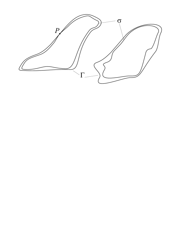
Figure 3: The $\Gamma$ and the leminscate $\sigma$ as in the second half of Proposition 5.1

Note that in (5.3) the inequality $\omega_{\sigma}(P)\leq\omega_{\Gamma}(P)$ is automatic since $\Gamma$ lies inside $\sigma$. In a similar way, in (5.4) the inequality $\omega_{\Gamma}(P)\leq\omega_{\sigma}(P)$ holds.

Actually, in [11] the conditions (5.3) and (5.4) were formulated in terms of the normal derivatives of the Green’s function of the outer domains to $\Gamma$ and $\sigma$, but, in view of the fact that this latter is just $2\pi$-times the equilibrium density (see [14, II.(4.1)] or [17, Theorem IV.2.3] and [17, (I.4.8)]), the two formulations are equivalent.

5.1 The lower estimate

Let $P_{n}$ be the extremal polynomial for $\lambda_{n}(\mu,z_{0})$, and for some $\tau>0$ let $S_{\tau n,z_{0},K}$ be the fast decreasing polynomial given by Proposition 2.1 with some $\gamma>1$ to be chosen below, where $K$ is the set enclosed by $\Gamma$. Let $\sigma=\sigma_{z_{0}}$ be a lemniscate inside $\Gamma$ given by the second part of Proposition 5.1, and suppose that $\sigma=\{z:|T_{N}(z)|=1\}$, where $T_{N}$ is a polynomial of degree $N$ and $T_{N}(z_{0})=e^{i\pi/2}$. Define $R_{n}=P_{n}S_{\tau n,z_{0},K}$. Note that $R_{n}$ is a polynomial of degree at most $(1+\tau)n$ and $R_{n}(z_{0})=1$. These will be the test polynomials in estimating the Christoffel function for the measure

$$d\mu_{\sigma}(z):=|z-z_{0}|^{\alpha}ds_{\sigma}(z)$$

on $\sigma$, but first we need two nontrivial facts for these polynomials.

Lemma 5.2

Let $\frac{1}{2}<\beta<1$ be fixed. For $z\in\Gamma$ such that $|z-z_{0}|\leq 2n^{-\beta}$, let $z^{*}\in\sigma$ be the point such that $s_{\sigma}([z_{0},z^{*}])=s_{\Gamma}([z_{0},z])$ holds (actually, there are two such points, we choose as $z^{*}$ the one the lies closer to $z$). Then the mapping $q(z)=z^{*}$ is one to one, $|q(z)-z|\leq C|z-z_{0}|^{2}$, $ds_{\Gamma}(z)=ds_{\sigma}(z^{*})$, $|q^{\prime}(z_{0})|=1$, and with the notation $I_{n}:=\{z^{*}\in\sigma:|z^{*}-z_{0}|\leq n^{-\beta}\}$, we have

$$\Bigg{|}\int_{z^{*}\in I_{n}}|R_{n}(z^{*})|^{2}|z-z_{0}|^{\alpha}ds_{\sigma}(z^{*})-\int_{z^{*}\in I_{n}}|R_{n}(z)|^{2}|z-z_{0}|^{\alpha}ds_{\Gamma}(z)\Bigg{|}=o(n^{-(1+\alpha)}).$$ (5.5)

On the left-hand side $z=q^{-1}(z^{*})$, so the integrand is a function of $z^{*}$.

Proof.  First of all we mention that $|q^{\prime}(z_{0})|=1$, i.e. for every $\varepsilon>0$, if $|z-z_{0}|$ is small enough, then

$$1-\varepsilon\leq\frac{|q(z)-z_{0}|}{|z-z_{0}|}\leq 1+\varepsilon,$$

which is clear since $q(z)=z+O(|z-z_{0}|^{2})$.

We proceed to prove (5.5).

$$\Bigg{|}\int_{z^{*}\in I_{n}}|R_{n}(z^{*})|^{2}|z-z_{0}|^{\alpha}ds_{\sigma}(z^{*})-\int_{z^{*}\in I_{n}}|R_{n}(z)|^{2}|z-z_{0}|^{\alpha}ds_{\Gamma}(z)\Bigg{|}$$

$$\leq\Bigg{|}\int_{z^{*}\in I_{n}}\Big{(}|R_{n}(z^{*})|^{2}-|R_{n}(z)|^{2}\Big{)}|z-z_{0}|^{\alpha}ds_{\Gamma}(z)\Bigg{|}$$

$$\leq\int_{z^{*}\in I_{n}}\Big{|}|R_{n}(z^{*})|^{2}-|R_{n}(z)|^{2}\Big{|}|z-z_{0}|^{\alpha}ds_{\Gamma}(z):=A.$$

Using the Hölder and Minkowski inequalities we can continue as

$$A \leq \Bigg{(}\int_{z^{*}\in I_{n}}|R_{n}(z^{*})-R_{n}(z)|^{2}|z-z_{0}|^{\alpha}ds_{\Gamma}(z)\Bigg{)}^{1/2}\times$$

$$\Bigg{\{}\Bigg{(}\int_{z^{*}\in I_{n}}|R_{n}(z^{*})|^{2}|z-z_{0}|^{\alpha}ds_{\Gamma}(z)\Bigg{)}^{1/2}+\Bigg{(}\int_{z^{*}\in I_{n}}|R_{n}(z)|^{2}|z-z_{0}|^{\alpha}ds_{\Gamma}(z)\Bigg{)}^{1/2}\Bigg{\}}.$$

We estimate these integrals term by term.

$P_{n}$ is extremal for $\lambda_{n}(\mu,z_{0})=O(n^{-(\alpha+1)})$ (see Lemma 2.9), therefore we have (use also that $|R_{n}(z)|\leq|P_{n}(z)|$)

$$\Bigg{(}\int_{z^{*}\in I_{n}}|R_{n}(z)|^{2}|z-z_{0}|^{\alpha}ds_{\Gamma}(z)\Bigg{)}^{1/2}\leq Cn^{-\frac{\alpha+1}{2}}.$$ (5.7)

This takes care of the third term in (5.1).

The estimates for the other two terms differ in the cases $\alpha\geq 0$ and $\alpha<0$.

Assume first that $\alpha\geq 0$. From Lemma 2.7, we get for any closed subarc $J_{1}\subset J$

$$\|R_{n}\|_{J_{1}}\leq Cn^{(\alpha+1)/2}\|R_{n}\|_{L^{2}(\mu)}\leq C,$$

where we used Lemma 2.9 and $|R_{n}(z)|\leq|P_{n}(z)|$. Choose this $J_{1}$ so that it contains $z_{0}$ in its interior. Next, note that if $z^{*}\in I_{n}$, then $|z^{*}-z|\leq Cn^{-2\beta}$, so dist$(z^{*},z)\leq C/n$. Therefore, an application of Lemma 2.4 yields for such $z$

$$\frac{|R_{n}(q(z))-R_{n}(z)|}{|q(z)-z|}\leq Cn\|R_{n}\|_{J_{1}},$$

and so

$$|R_{n}(q(z))-R_{n}(z)|\leq Cn|q(z)-z|\leq Cn^{1-2\beta}.$$ (5.8)

Since $s_{\sigma}(I_{n})\leq Cn^{-\beta}$ is also true, we have (recall that $z^{*}=q(z)$)

$$\Bigg{(}\int_{z^{*}\in I_{n}}|R_{n}(z^{*})-R_{n}(z)|^{2}|z-z_{0}|^{\alpha}ds_{\Gamma}(z)\Bigg{)}^{1/2} \leq C\Big{(}n^{-\beta}n^{2-4\beta}n^{-\alpha\beta}\Big{)}^{1/2}$$

$$= Cn^{1-\frac{5+\alpha}{2}\beta}.$$

This is the required estimate for the first term in (5.1).

Finally, for the middle term in (5.1), we have

$$\Bigg{(}\int_{z^{*}\in I_{n}}|R_{n}(z^{*})|^{2} |z-z_{0}|^{\alpha}ds_{\Gamma}(z)\Bigg{)}^{1/2}$$

$$=\Bigg{(}\int_{z^{*}\in I_{n}}\Big{|}|R_{n}(z^{*})|^{2}-|R_{n}(z)|^{2}+|R_{n}(z)|^{2}\Big{|}|z-z_{0}|^{\alpha}ds_{\Gamma}(z)\Bigg{)}^{1/2}$$

$$\leq\Bigg{(}\int_{z^{*}\in I_{n}}\Big{|}|R_{n}(z^{*})|^{2}-|R_{n}(z)|^{2}\Big{|}|z-z_{0}|^{\alpha}ds_{\Gamma}(z)\Bigg{)}^{1/2}$$

$$\phantom{aaaaaaaaaaaaa}+\Bigg{(}\int_{z^{*}\in I_{n}}|R_{n}(z)|^{2}|z-z_{0}|^{\alpha}ds_{\Gamma}(z)\Bigg{)}^{1/2}$$

$$\leq A^{1/2}+Cn^{-\frac{\alpha+1}{2}},$$

where $A$ is the left-hand side in (5.1), and where we also used (5.7).

Combining these we get

$$A \leq Cn^{1-\frac{5+\alpha}{2}\beta}\Big{(}A^{1/2}+Cn^{-\frac{\alpha+1}{2}}\Big{)}\leq CA^{1/2}n^{1-\frac{5+\alpha}{2}\beta}+Cn^{\frac{1}{2}-\frac{\alpha}{2}-\frac{5+\alpha}{2}\beta}$$

$$\leq C\max\{A^{1/2}n^{1-\frac{5+\alpha}{2}\beta},n^{\frac{1}{2}-\frac{\alpha}{2}-\frac{5+\alpha}{2}\beta}\}.$$

Therefore $A\leq Cn^{2-(5+\alpha)\beta}$ or $A\leq Cn^{\frac{1}{2}-\frac{\alpha}{2}-\frac{5+\alpha}{2}\beta}$. If $\beta<1$ is sufficiently close to $1$, then both imply $A=o(n^{-(\alpha+1)})$.

Now assume that $\alpha<0$. From Lemma 2.7, we get for any closed subarc $J_{1}\subset J$

$$\|R_{n}\|_{J_{1}}\leq\|P_{n}\|_{J_{1}}\leq Cn^{1/2}\|P_{n}\|_{L^{2}(\mu)}\leq Cn^{-\alpha/2},$$

and we may assume that here $J_{1}$ is such that it contains a neighborhood of $z_{0}$. Therefore, in this case (5.8) takes the form

$$|R_{n}(z^{*})-R_{n}(z)|\leq Cn^{1-\alpha/2-2\beta}.$$

Since

$$\int_{z^{*}\in I_{n}}|z-z_{0}|^{\alpha}ds_{\Gamma}(z)\leq Cn^{-\alpha\beta-\beta},$$

we obtain

$$\Bigg{(}\int_{z^{*}\in I_{n}}|R_{n}(z^{*})-R_{n}(z)|^{2} |z-z_{0}|^{\alpha}ds_{\Gamma}(z)\Bigg{)}^{1/2}\leq Cn^{1-\frac{\alpha}{2}-2\beta-\frac{(\alpha+1)}{2}\beta},$$

which is the required estimate for the first term in (5.1). Finally, for the middle term in (5.1) we get, similarly as before,

$$\Bigg{(}\int_{z^{*}\in I_{n}}|R_{n}(z^{*})|^{2} |z-z_{0}|^{\alpha}ds_{\Gamma}(z)\Bigg{)}^{1/2}\leq A^{1/2}+Cn^{-\frac{\alpha+1}{2}}.$$

As previously, we can conclude from these

$$A\leq Cn^{1-\frac{\alpha}{2}-2\beta-\frac{\alpha+1}{2}\beta}(A^{1/2}+n^{-\frac{\alpha+1}{2}}),$$

which implies

$$A\leq C\max\{n^{2-\alpha-4\beta-(\alpha+1)\beta},n^{\frac{1}{2}-\alpha-2\beta-\frac{\alpha+1}{2}\beta}\}.$$

If $\beta$ is sufficiently close to $1$, then this yields again $A=o(n^{-(\alpha+1)})$, as needed.  

In what follows we keep the notations from the preceding proof. In the following lemma let $\Delta_{\delta}(z_{0})=\{z\;:\;|z-z_{0}|\leq\delta\}$ be the disk about $z_{0}$ of radius $\delta$.

Note that up to this point the $\gamma>1$ in Proposition 2.1 was arbitrary. Now we specify how close it should be to 1.

Lemma 5.3

If $0<\beta<1$ is fixed and $\gamma>1$ is chosen so that $\beta\gamma<1$, then

$$\|R_{n}\|_{K\setminus\Delta_{n^{-\beta}/2}}(z_{0})=o(n^{-1-\alpha}).$$ (5.9)

Recall that here $K$ is the set enclosed by $\Gamma$.

Proof.  Let us fix a $\delta>0$ such that the intersection $\Gamma\cap\Delta_{\delta}(z_{0})$ lies in the interior of the arc $J$ from Theorem 1.1. By $\mu\in{\bf Reg}$ and the trivial estimate $\|P_{n}\|_{L^{2}(\mu)}=O(1)$ we get that no matter how small $\varepsilon>0$ is given, for sufficiently large $n$ we have $\|P_{n}\|_{\Gamma}\leq(1+\varepsilon)^{n}$. On the other hand, in view of Proposition 2.1, we have for $z\not\in\Delta_{\delta}(z_{0})$, $z\in K$,

$$|S_{\tau n,z_{0},K}(z)|\leq C_{\gamma}e^{-c_{\gamma}\tau n\delta^{2}},$$

so

$$\|R_{n}\|_{K\setminus\Delta_{\delta}}(z_{0})=o(n^{-1-\alpha})$$ (5.10)

certain holds.

Consider now $K\cap\Delta_{\delta}(z_{0})$. Its boundary consists of the arc $\Gamma\cap\Delta_{\delta}(z_{0})$, which is part of $J$, and of an arc on the boundary of $\Delta_{\delta}(z_{0})$, where we already know the bound (5.10). On the other hand, on $\Gamma\cap\Delta_{\delta}(z_{0})$ we have, by Lemma 2.7,

$$|P_{n}(z)|\leq Cn^{(1+|\alpha|)/2}\|P_{n}\|_{L^{2}(\mu)}\leq Cn^{(1+|\alpha|)/2}.$$

Therefore, by the maximum principle, we obtain the same bound (for large $n$) on the whole set $K\cap\Delta_{\delta}(z_{0})$. As a consequence, for $z\in K\setminus\Delta_{n^{-\beta}/2}$

$$|R_{n}(z)|\leq Cn^{(1+|\alpha|)/2}e^{-c_{\gamma}\tau n(n^{-\beta}/2)^{\gamma}}=o(n^{-1-\alpha})$$

if we choose $\gamma>1$ in Proposition 2.1 so that $\beta\gamma<1$. These prove (5.9).  

After these preliminaries we return to the proof of Theorem 1.1, more precisely to the lower estimate of $\lambda_{n}(\mu,z_{0})$.

Let $\eta>0$ be arbitrary, and let $n$ be so large that

$$\frac{1}{1+\eta}w(z_{0})\leq w(z)\leq(1+\eta)w(z_{0}),\qquad\frac{1}{1+\eta}|z-z_{0}|\leq|q(z)-z_{0}|\leq(1+\eta)|z-z_{0}|$$

hold for all $z^{*}\in I_{n}$, where $I_{n}$ is the set from Lemma 5.2. Then we obtain from Lemma 5.2 (recall that $z^{*}=q(z)$)

$$\int_{z^{*}\in I_{n}}|R_{n}(z^{*})|^{2} |z^{*}-z_{0}|^{\alpha}ds_{\sigma}(z^{*})$$

$$\leq(1+\eta)^{|\alpha|}\int_{z^{*}\in I_{n}}|R_{n}(z^{*})|^{2}|z-z_{0}|^{\alpha}ds_{\Gamma}(z)$$

$$\leq(1+\eta)^{|\alpha|}\int_{z^{*}\in I_{n}}|R_{n}(z)|^{2}|z-z_{0}|^{\alpha}ds_{\Gamma}(z)+o(n^{-(\alpha+1)})$$

$$\leq\frac{(1+\eta)^{|\alpha|+1}}{w(z_{0})}\int_{z^{*}\in I_{n}}|R_{n}(z)|^{2}w(z)|z-z_{0}|^{\alpha}ds_{\Gamma}(z)+o(n^{-(\alpha+1)})$$

$$\leq\frac{(1+\eta)^{|\alpha|+1}}{w(z_{0})}\lambda_{n}(\mu,z_{0})+o(n^{-(\alpha+1)}).$$

On the other hand, if we notice that if, for some $z\in\sigma$, we have $z^{*}\not\in I_{n}$ then necessarily $|z-z_{0}|\geq n^{-\beta}/2$, we obtain from Lemma 5.3

$$\int_{z^{*}\in\sigma\setminus I_{n}}|R_{n}(z^{*})|^{2} |z^{*}-z_{0}|^{\alpha}ds_{\sigma}(z^{*})=o(n^{-(1+\alpha)}).$$

Combining these, it follows that

$$\lambda_{\deg(R_{n})}(\mu_{\sigma},z_{0}) \leq \int_{z\in\sigma}|R_{n}(z^{*})|^{2}|z^{*}-z_{0}|^{\alpha}ds_{\sigma}(z^{*})$$

$$\leq \frac{(1+\eta)^{|\alpha|+1}}{w(z_{0})}\lambda_{n}(\mu,z_{0})+o(n^{-(\alpha+1)}).$$

Since $\deg(R_{n})\leq(1+\tau)n$, we can conclude from (4.6) (see also (2.1))

$$\frac{L_{\alpha}}{(\pi\omega_{\sigma}(z_{0}))^{\alpha+1}} = \liminf_{n\to\infty}\deg(R_{n})^{\alpha+1}\lambda_{\deg(R_{n})}(\mu_{\sigma},z_{0})$$

$$\leq \liminf_{n\to\infty}(1+\tau)^{\alpha+1}\frac{(1+\eta)^{|\alpha|+1}}{w(z_{0})}n^{\alpha+1}\lambda_{n}(\mu,z_{0}).$$

But here $\tau,\eta>0$ are arbitrary, so we get

$$\liminf_{n\to\infty}n^{\alpha+1}\lambda_{n}(\mu,z_{0})\geq\frac{w(z_{0})}{(\pi\omega_{\sigma}(z_{0}))^{\alpha+1}}L_{\alpha}.$$

As $\omega_{\sigma}(z_{0})\leq\omega_{\Gamma}(z_{0})+\varepsilon$ (see (5.4)), for $\varepsilon\to 0$ we finally arrive at the lower estimate

$$\liminf_{n\to\infty}n^{\alpha+1}\lambda_{n}(\mu,z_{0})\geq\frac{w(z_{0})}{(\pi\omega_{\Gamma}(z_{0}))^{\alpha+1}}L_{\alpha}.$$ (5.11)

5.2 The upper estimate

Let now $\sigma$ be the lemniscate given by the first part of Proposition 5.1, and let $P_{n}$ be the polynomial extremal for $\lambda_{n}(\mu_{\sigma},z_{0})$. Define, with some $\tau>0$,

$$R_{n}(z)=P_{n}(z)S_{\tau n,z_{0},L}(z),$$

where $S_{\tau n,z_{0},L}$ is the fast decreasing polynomial given by Proposition 2.1 for the lemniscate set $L$ enclosed by $\sigma$ (with some $\gamma>1$). Let $\eta>0$ be arbitrary, $\frac{1}{2}<\beta<1$ as before, and suppose that $n$ is so large such that

$$\frac{1}{1+\eta}w(z_{0}) \leq w(z)\leq(1+\eta)w(z_{0})$$

$$\frac{1}{\eta+1} \leq|q^{\prime}(z)|\leq(1+\eta)$$

$$\frac{1}{1+\eta}|z-z_{0}| \leq|q(z)-z_{0}|\leq(1+\eta)|z-z_{0}|$$

are true for all $|z-z_{0}|\leq n^{-\beta}$. Using Lemma 5.2 (more precisely its version when $\sigma$ encloses $\Gamma$) we have (recall again that $z^{*}=q(z)$)

$$\int_{z^{*}\in I_{n}}|R_{n}(z)|^{2} w(z)|z-z_{0}|^{\alpha}ds_{\Gamma}(z)$$

$$\leq(1+\eta)w(z_{0})\int_{z^{*}\in I_{n}}|R_{n}(z)|^{2}|z-z_{0}|^{\alpha}ds_{\Gamma}(z)$$

$$\leq(1+\eta)w(z_{0})\int_{z^{*}\in I_{n}}|R_{n}(z^{*})|^{2}|z-z_{0}|^{\alpha}ds_{\sigma}(z^{*})+o(n^{-(\alpha+1)})$$

$$\leq(1+\eta)^{|\alpha|+1}w(z_{0})\int_{z^{*}\in I_{n}}|R_{n}(z^{*})|^{2}|z^{*}-z_{0}|^{\alpha}ds_{\sigma}(z^{*})+o(n^{-(\alpha+1)})$$

$$\leq(1+\eta)^{|\alpha|+1}w(z_{0})\lambda_{n}(\mu_{\sigma},z_{0})+o(n^{-(\alpha+1})).$$

On the other hand, Lemma 5.3 (but now applied for the system of curves $\sigma$ rather than for $\Gamma$) implies, as before,

$$\int_{\Gamma\setminus\Delta_{n^{-\beta}/2}(z_{0})}|R_{n}(z)|^{2}|z-z_{0}|^{\alpha}d\mu(z)=o(n^{-(1+\alpha)}).$$

Therefore,

$$\lambda_{\deg(R_{n})}(\mu,z_{0})\leq(1+\eta)^{|\alpha|+1}w(z_{0})\lambda_{n}(\mu_{\sigma},z_{0})+o(n^{-(\alpha+1)}),$$

which, similarly to the lower estimate, upon using (4.6) and letting $\tau,\eta$ tend to zero, implies (see also (2.2))

$$\limsup_{n\to\infty}n^{\alpha+1}\lambda_{n}(\mu,z_{0}) \leq\frac{w(z_{0})}{(\pi\omega_{\sigma}(z_{0}))^{\alpha+1}}L_{\alpha}.$$

Here, in view of (5.3), $\omega_{\Gamma}(z_{0})\leq\omega_{\sigma}(z_{0})+\varepsilon$, hence for $\varepsilon\to 0$ we conclude

$$\limsup_{n\to\infty}n^{\alpha+1}\lambda_{n}(\mu,z_{0}) \leq\frac{w(z_{0})}{(\pi\omega_{\Gamma}(z_{0}))^{\alpha+1}}L_{\alpha}.$$

This and (5.11) prove (5.2).  

6 Piecewise smooth Jordan curves

The proof in the preceding section can be carried out without any difficulty if $\Gamma$ consists of piecewise $C^{2}$-smooth Jordan curves, provided that in a neighborhood of $z_{0}$ the $\Gamma$ is $C^{2}$-smooth. Indeed, in that case we can still talk about $\omega_{\Gamma}$ which is continuous where $\Gamma$ is $C^{2}$-smooth (see [24, Proposition 2.2]), and in the above proof the $C^{2}$-smoothness was used only in a neighborhood of $z_{0}$. Therefore, we have

Proposition 6.1

Let $\Gamma$ consist of finitely many disjoint, piecewise $C^{2}$-smooth Jordan curves. Let $z_{0}\in\Gamma$, and in a neighborhood of $z_{0}\in\Gamma$ let $\Gamma$ be $C^{2}$-smooth. Then, for the measure $\mu$ given in (5.1), we have (5.2).

7 Arc components

In this section, we prove Theorem 1.1 when $\Gamma$ is a union of $C^{2}$-smooth Jordan curves and arcs, and $\mu$ is the measure (5.1) considered before. To be more specific, our aim is to verify

Proposition 7.1

Let $\Gamma$ consist of finitely many disjoint $C^{2}$-smooth Jordan curves or arcs lying exterior to each other, and let $z_{0}\in\Gamma$. Assume that in a neighborhood of the point $z_{0}\in\Gamma$, the $\Gamma$ is $C^{2}$-smooth, and $z_{0}$ is not an endpoint of an arc component of $\Gamma$. Then, for the measure (5.1) where $w$ is continuous and positive and $\alpha>-1$, we have (1.4).

We shall need some facts about Bessel functions, and a discretization of the equilibrium measure $\nu_{\Gamma}$ that uses the zeros of an appropriate Bessel function.

7.1 Bessel functions and some local asymptotics

We shall need the Bessel function of the first kind of order $\beta>0$:

$$J_{\beta}(z)=\sum_{n=0}^{\infty}\frac{(-1)^{n}(z/2)^{2n+\beta}}{n!\Gamma(n+\beta+1)},$$

as well as the functions (c.f. [10])

$$\mathbb{J}_{\beta}(u,v)=\frac{J_{\beta}(\sqrt{u})\sqrt{v}J_{\beta}^{\prime}(\sqrt{v})-J_{\beta}(\sqrt{v})\sqrt{u}J_{\beta}^{\prime}(\sqrt{u})}{2(u-v)},$$

$$\mathbb{J}_{\beta}^{*}(z)=\frac{{J}_{\beta}(z)}{z^{\beta}},\qquad\mathbb{J}_{\beta}^{*}(u,v)=\frac{\mathbb{J}_{\beta}(u,v)}{u^{\beta/2}v^{\beta/2}}.$$

These latter ones are analytic, and we have

$$\mathbb{J}_{\beta}^{*}(u,0)=\frac{1}{2^{2\beta+1}u}\sum_{n=1}^{\infty}\frac{(-1)^{n}(\sqrt{u}/2)^{2n}}{n!\Gamma(n+\beta+1)}\left(\frac{\beta}{\Gamma(\beta+1)}-\frac{2n+\beta}{\Gamma(\beta+1)}\right)=\frac{\mathbb{J}^{*}_{\beta+1}(\sqrt{u})}{2^{\beta+1}\Gamma(\beta+1)}.$$

Let $d\nu_{0}(x)$ be the measure $x^{\beta}dx$ with support $[0,2]$, and $K_{n}^{(0)}(x,t)$ its $n$-th reproducing kernel. It is known (see [9, (1.2)] or [20, (4.5.8), p. 72]) that

$$\frac{K_{n}^{(0)}\left(\frac{x^{2}}{2n^{2}},0\right)}{K_{n}^{(0)}(0,0)}=(1+o(1))\frac{\mathbb{J}_{\beta}^{*}(x^{2},0)}{\mathbb{J}_{\beta}^{*}(0,0)},$$

which holds uniformly for $|x|\leq A$ with any fixed $A$. We have already mentioned (see e.g. [20, Theorem 3.1.3]) that the polynomial $K_{n}^{(0)}(t,0)/K_{n}^{(0)}(0,0)$ is the extremal polynomial of degree $n$ for $\lambda_{n}(\nu_{0},0)$, so the preceding relation gives an asymptotic formula for this extremal polynomial on intervals $[0,A/n^{2}]$. If now $d\nu_{1}(x)=(2x)^{\beta}dx$ but with support $[0,1]$, and $K_{n}^{(1)}$ is the associated reproducing kernel, then $K_{n}^{(1)}(t,0)/K_{n}^{(1)}(0,0)$ is the extremal polynomial of degree $n$ for $\lambda_{n}(\nu_{1},0)$, and it is clear that this is just a scaled version of the extremal polynomial for $\nu_{0}$:

$$\frac{K_{n}^{(1)}(t,0)}{K_{n}^{(1)}(0,0)}=\frac{K_{n}^{(0)}(2t,0)}{K_{n}^{(0)}(0,0)}.$$

Therefore,

$$\frac{K_{n}^{(1)}\left(\frac{x^{2}}{4n^{2}},0\right)}{K_{n}^{(1)}(0,0)}=(1+o(1))\frac{\mathbb{J}_{\beta}^{*}(x^{2},0)}{\mathbb{J}_{\beta}^{*}(0,0)}.$$

Then the same is true for the measure $2^{-\beta}d\nu_{1}(x)=x^{\beta}dx$ with support $[0,1]$ (multiplying the measure by a constant does not change the extremal polynomial for the Christoffel functions). Next, consider the measure $d\nu_{2}(x)=|x|^{\alpha}dx$ with support $[-1,1]$. For this the extremal polynomial for $\lambda_{2n}(\nu_{2},0)$ is obtained from the extremal polynomial for $\lambda_{n}(\nu_{1},0)$ with $\beta=(\alpha-1)/2$ by the substitution $t\to t^{2}$ (see Section 3.1, in particular see the last paragraph in that section), i.e.

$$\frac{K_{2n}^{(2)}\left(t,0\right)}{K_{2n}^{(2)}(0,0)}=\frac{K_{n}^{(1)}\left(t^{2},0\right)}{K_{n}^{(1)}(0,0)}.$$

Hence, for even integers $n$

$$\frac{K_{n}^{(2)}\left(t,0\right)}{K_{n}^{(2)}(0,0)}=(1+o(1)){\cal J}_{\frac{\alpha+1}{2}}(nt),\qquad|t|\leq\frac{A}{n},$$

where

$${\cal J}_{\frac{\alpha+1}{2}}(z):=\frac{\mathbb{J}_{\frac{\alpha-1}{2}}^{*}(z^{2},0)}{\mathbb{J}_{\frac{\alpha-1}{2}}^{*}(0,0)}=\frac{\mathbb{J}_{\frac{\alpha+1}{2}}^{*}(z)}{\mathbb{J}_{\frac{\alpha+1}{2}}^{*}(0)}.$$ (7.1)

Fix a positive number $A$. According to what we have just seen, for every even $n$

$$\int_{-A/n}^{A/n}{\cal J}_{\frac{\alpha+1}{2}}(nt)^{2}|t|^{\alpha}dt \leq (1+o(1))\int_{-A/n}^{A/n}\left(\frac{K_{n}^{(2)}\left(t,0\right)}{K_{n}^{(2)}(0,0)}\right)^{2}|t|^{\alpha}dt$$

$$\leq (1+o(1))\lambda_{n}(\nu_{2},0),$$

and so for any (even) $n$

$$\int_{-A}^{A}{\cal J}_{\frac{\alpha+1}{2}}(x)^{2}|x|^{\alpha}dx=n^{\alpha+1}\int_{-A/n}^{A/n}{\cal J}_{\frac{\alpha+1}{2}}(nt)^{2}|t|^{\alpha}dt\leq(1+o(1))n^{\alpha+1}\lambda_{n}\left(\nu_{2},0\right).$$

Now if we let here $n\to\infty$ and use the limit (3.3) for the right-hand side, then we obtain

$$\int_{-A}^{A}{\cal J}_{\frac{\alpha+1}{2}}(x)^{2}|x|^{\alpha}dx\leq L_{\alpha},$$

where $L_{\alpha}$ is from (3.4). Finally, since here $A$ is arbitrary, we can conclude

$$\int_{-\infty}^{\infty}{\cal J}_{\frac{\alpha+1}{2}}(x)^{2}|x|^{\alpha}dx\leq L_{\alpha}.$$ (7.2)

7.2 The upper estimate in Theorem 1.1 for one arc

The aim of this section is to construct polynomials that verify the upper estimate for the Christoffel functions in Theorem 1.1 (which is the same as in Proposition 7.1) when $\Gamma$ consists of a single $C^{2}$-smooth arc, and $z_{0}\in\Gamma$ is not an endpoint of that arc. In the next subsection we shall indicate what to do when $\Gamma$ has other components, as well.

Let $\nu_{\Gamma}$ be the equilibrium measure of $\Gamma$ and $s_{\Gamma}$ the arc measure on $\Gamma$. Since $\Gamma$ is assumed to be $C^{2}$-smooth, we have $d\nu_{\Gamma}(t)=\omega_{\Gamma}(t)ds_{\Gamma}(t)$ with an $\omega_{\Gamma}$ that is continuous and positive away from the endpoints of $\Gamma$ (see [24, Proposition 2.2]).

We may assume $z_{0}=0$ and that the real line is the tangent line to $\Gamma$ at the origin. By assumption, the measure $\mu$ we are dealing with, is, in a neighborhood of the origin, of the form $d\mu(z)=w(z)|z|^{\alpha}ds_{\Gamma}(z)$ with some positive and continuous function $w(z)$.

Since $\Gamma$ is assumed to be $C^{2}$-smooth, in a neighborhood of the origin we have the parametrization $\gamma(t)=\gamma_{1}(t)+i\gamma_{2}(t)$, $\gamma_{1}(t)\equiv t$, where $\gamma_{2}$ is a twice continuously differentiable function such that $\gamma_{2}(0)=\gamma_{2}^{\prime}(0)=0$. In particular, as $t\to 0$ we have $\gamma_{2}(t)=O(t^{2})$, $\gamma_{2}^{\prime}(t)=O(|t|)$. We shall also take an orientation of $\Gamma$, and we shall denote $z\prec w$ if $z\in\Gamma$ precedes $w\in\Gamma$ in that orientation. We may assume that this orientation is such that around the origin we have $z\prec w\Leftrightarrow\Re z<\Re w$.

It is known that, when dealing with $|z|^{\alpha}$ weights on the real line, Bessel functions of the first kind enter the picture, see [7], [9], [10]. For a given large $n$ we shall construct the necessary polynomials from two sources: from points on $\Gamma$ that follow the pattern of the zeros of the Bessel function ${\cal J}_{\frac{\alpha+1}{2}}$, and from points that are obtained from discretizing the equilibrium measure $\nu_{\Gamma}$. The first type will be used close to the origin (of distance $\leq 1/n^{\tau}$ with some appropriate $\tau$), while the latter type will be on the rest of $\Gamma$. So first we shall discuss two different divisions of $\Gamma$.

7.2.1 Division based on the zeros of Bessel functions

Let $\beta=\frac{\alpha+1}{2}$ — it is a positive number because $\alpha>-1$. It is known that $J_{\beta}$, and hence also ${\cal J}_{\beta}$ from (7.1), has infinitely many positive zeros which are all simple and tend to infinity, let them be $j_{\beta,1}<j_{\beta,2}<\ldots$. We have the asymptotic formula (see [28, 15.53])

$$j_{\beta,k}=(k+\frac{\beta}{2}-\frac{1}{4})\pi+o(1),\qquad k\to\infty.$$ (7.3)

The negative zeros of ${\cal J}_{\beta}$ are $-j_{\beta,k}$, and we have the product formula (see [28, 15.41,(3)])

$$J_{\beta}(z)=\frac{(z/2)^{\beta}}{\Gamma(\beta+1)}\prod_{k=1}^{\infty}\left(1-\frac{z^{2}}{j_{\beta,k}^{2}}\right).$$

Therefore,

$${\cal J}_{\beta}(z)=\prod_{k=1}^{\infty}\left(1-\frac{z^{2}}{j_{\beta,k}^{2}}\right).$$ (7.4)

Let $a_{0}=0$, and for $k>0$ let $a_{k}\in\Gamma$ be the unique point on $\Gamma$ such that $0\prec a_{k}$, and

$$\nu_{\Gamma}(\overline{0a_{k}})=\frac{j_{\beta,k}}{\pi n},$$ (7.5)

where $\overline{0a_{k}}$ denotes the arc of $\Gamma$ that lies in between $0$ and $a_{k}$. For negative $k$ let similarly $a_{k}$ be the unique number for which $a_{k}\prec 0$ and

$$\nu_{\Gamma}(\overline{a_{k}0})=\frac{j_{\beta,|k|}}{\pi n}.$$ (7.6)

The reader should be aware that these $a_{k}$ and the whole division depends on $n$, so a more precise notation would be $a_{k,n}$ for $a_{k}$, but we shall suppress the additional parameter $n$.

This definition makes sense only for finitely many $k$, say for $-k_{0}<k<k_{1}$, and in view of (7.3) we have $k_{0}+k_{1}=n+O(1)$, i.e. there are about $n$ such $a_{k}$ on $\Gamma$. The arcs $\overline{a_{k}a_{k+1}}$ are subarcs of $\Gamma$ that follow each other according to $\prec$, for them

$$\nu_{\Gamma}(\overline{a_{k-1}a_{k}})=\frac{j_{\beta,k}-j_{\beta,k-1}}{\pi n},\qquad k>0,$$

$$\nu_{\Gamma}(\overline{a_{k-1}a_{k}})=\frac{j_{\beta,k+1}-j_{\beta,k}}{\pi n},\qquad k<0,$$

and their union is almost the entire $\Gamma$: there can be two additional arcs around the two endpoints with equilibrium measure $<(j_{\beta,k_{0}}-j_{\beta,k_{0}-1})/\pi n$ resp. $<(j_{\beta,k_{1}}-j_{\beta,k_{1}-1})/\pi n$.

7.2.2 Division based solely on the equilibrium measure

In this subdivision of $\Gamma$ we follow the procedure in [24, Section 2]. Let $\overline{b_{0}b_{1}}\subset\Gamma$ be the unique arc (at least for large $n$ it is unique) with the property that $0\in\overline{b_{0}b_{1}}$, $\nu_{\Gamma}(\overline{b_{0}b_{1}})=1/n$, and if $\xi_{0}$ is the center of mass of $\nu_{\Gamma}$ on $\overline{b_{0}b_{1}}$, then $\Re\xi_{0}=0$. For $k>1$ let $b_{k}\in\Gamma$ be the point on $\Gamma$ (if there is one) with the property that $0\prec b_{k}$ and $\nu_{\Gamma}(\overline{b_{1}b_{k}})=(k-1)/n$, and similarly, for negative $k$ let $b_{k}\prec 0$ be the point on $\Gamma$ with the property $\nu_{\Gamma}(\overline{b_{k}b_{0}})=|k|/n$. This definition makes sense only for finitely many $k$, say for $-l_{0}<k<l_{1}$. Thus, the arcs $\overline{b_{k}b_{k+1}}$, $-l_{0}<k<l_{1}-1$, continuously fill $\Gamma_{0}$ (in the orientation of $\Gamma_{0}$) and they all have equal, $1/n$ weight with respect to the equilibrium measure $\nu_{\Gamma}$. It may happen that, with this selection, around the endpoints of $\Gamma$ there still remain two “little” arcs, say $\overline{b_{-l_{0}}b_{-l_{0}+1}}$ and $\overline{b_{l_{1}-1}b_{l_{1}}}$ of $\nu_{\Gamma}$-measure $<1/n$. We include also these two small arcs into our subdivision of $\Gamma$, so in this case we divide $\Gamma$ into $n+1$ arcs $\overline{b_{k}b_{k+1}}$, $k=-l_{0},\ldots,l_{1}-1$.

Let $\xi_{k}$ be the center of mass of the measure $\nu_{\Gamma}$ on the arc $\overline{b_{k}b_{k+1}}$:

$$\xi_{k}=\frac{1}{\nu_{\Gamma}(\overline{b_{k}b_{k+1}})}\int_{\overline{b_{k}b_{k+1}}}u\;d\nu_{\Gamma}(u).$$ (7.7)

Since the length of $\overline{b_{k}b_{k+1}}$ is at most $C/n$ (note that $\omega_{\Gamma}$ has a positive lower bound), and $\Gamma$ is $C^{2}$-smooth, it follows that $\xi_{k}$ lies close to the arc $\overline{b_{k}b_{k+1}}$:

$${\rm dist}(\xi_{k},\overline{b_{k}b_{k+1}})\leq\frac{C}{n^{2}}$$ (7.8)

For the polynomials

$$B_{n}(z)=\prod_{k\not=0}(z-\xi_{k})$$ (7.9)

it was proven in [24, Propositions 2.4, 2.5] (see also [24, Section 2.2]) that $B_{n}(z)/B_{n}(0)$ are uniformly bounded on $\Gamma$:

$$\left|\frac{B_{n}(z)}{B_{n}(0)}\right|\leq C_{0},\qquad z\in\Gamma.$$ (7.10)

7.2.3 Construction of the polynomials ${\cal C}_{n}$

Choose a $0<\tau<1$ close to $1$ (we shall see later how close it has to be to 1), and for an $n$ define $N=N_{n}=[n^{3(1-\tau)}]$. We set

$${\cal C}_{n}(z)=:\prod_{k=-N_{n},\ k\not=0}^{N_{n}}\left(1-\frac{z}{a_{k}}\right)\prod_{|k|>N_{n}}\left(1-\frac{z}{\xi_{k}}\right).$$ (7.11)

Note that the precise range of $k$ in the second factor is $-l_{0}\leq k<-N_{n}$ as well as $N_{n}<k\leq l_{1}-1$. Since the number of all $\xi_{k}$ is $n+1$, this polynomial has degree $n$, and it takes the value 1 at the origin. This will be the main factor in the test polynomial that will give the appropriate upper bound for $\lambda_{n}(\mu,0)$, the other factor will be the fast decreasing polynomial from Corollary 2.2.

We estimate on $\Gamma$ the two factors

$${\cal A}_{n}(z):=\prod_{k=-N_{n},\ k\not=0}^{N_{n}}\left(1-\frac{z}{a_{k}}\right)$$

and

$${\cal B}_{n}(z):=\prod_{|k|>N_{n}}\left(1-\frac{z}{\xi_{k}}\right)$$

separately. The estimates will be distinctly different for $|z|\leq n^{-\tau}$ and for $|z|>n^{-\tau}$.

7.2.4 Bounds for ${\cal A}_{n}(z)$ for $|z|\leq n^{-\tau}$

In what follows, we shall use $N$ instead of $N_{n}$ ($=[n^{3(1-\tau)}]$).

Consider first

$${\cal A}_{n}^{*}(x):=\prod_{k=1}^{N}\left(1-\frac{(n\pi\omega_{\Gamma}(0)x)^{2}}{j_{\beta,k}^{2}}\right)$$

(recall that $j_{\beta,k}$ are the zeros of the Bessel function $J_{\beta}$ with $\beta=(\alpha+1)/2$). In view of (7.4) we can write for real $|x|\leq n^{-\tau}$

$$\frac{{\cal J}_{\beta}(n\pi\omega_{\Gamma}(0)x)}{{\cal A}_{n}^{*}(x)}=\prod_{k>N}\left(1-\frac{(n\pi\omega_{\Gamma}(0)x)^{2}}{j_{\beta,k}^{2}}\right).$$

Taking into account (7.3), here

$$\frac{n\pi\omega_{\Gamma}(0)x}{j_{\beta,k}}=O\left(\frac{nn^{-\tau}}{k}\right),$$

hence the product on the right is

$$\exp\left\{O\left(\sum_{k>N}\left(\frac{nn^{-\tau}}{k}\right)^{2}\right)\right\} = \exp\left(O\left(\frac{n^{2(1-\tau)}}{N}\right)\right)$$

$$= \exp\left(O\left(\frac{1}{n^{(1-\tau)}}\right)\right)=1+o(1).$$

Thus, our first estimate is

$${\cal A}_{n}^{*}(x)=(1+o(1)){\cal J}_{\beta}(n\pi\omega_{\Gamma}(0)x),\qquad|x|\leq n^{-\tau}.$$ (7.12)

Next, we go to a $z\in\Gamma$ with $|z|\leq n^{-\tau}$. Let $x$ be the real part of $z$. Then, for $|z|\leq n^{-\tau}$, we have (recall that $\Gamma$ is $C^{2}$-smooth and the real line is tangent to $\Gamma$)

$$z=x+O(x^{2})=x+O(n^{-2\tau}).$$

We shall need that the $a_{k}$’s with $|k|\leq N$ are close to $j_{\beta,k}/n\pi\omega_{\Gamma}(0)$. To prove that, consider the parametrization $\gamma(t)=t+i\gamma_{2}(t)$ of $\Gamma$ discussed in the beginning of this section. Then $a_{k}=\gamma(\Re a_{k})=\Re a_{k}+O((\Re a_{k})^{2})$. By the definition of the points $a_{k}$ we have for $1\leq k\leq N$

$$\frac{j_{\beta,k}}{\pi n}=\nu_{\Gamma}(\overline{0a_{k}})=\int_{0}^{\Re a_{k}}\omega_{\Gamma}(\gamma(t))|\gamma^{\prime}(t)|dt.$$ (7.13)

Now we use that around the origin $\omega_{\Gamma}$ is $C^{1}$-smooth (see [24, Proposition 2.2]), hence on the right

$$\omega_{\Gamma}(\gamma(t))=\omega_{\Gamma}(0)+O(|\gamma(t)|)=\omega_{\Gamma}(0)+O(|t|),$$

while

$$|\gamma^{\prime}(t)|=\sqrt{1+\gamma_{2}^{\prime}(t)^{2}}=\sqrt{1+O(t^{2})}=1+O(t^{2}),$$

hence

$$\frac{j_{\beta,k}}{\pi n}=\int_{0}^{\Re a_{k}}\left(\omega_{\Gamma}(0)+O(|t|)\right)dt=\omega_{\Gamma}(0)\Re a_{k}+O((\Re a_{k}))^{2},$$

which implies

$$\Re a_{k}=\frac{j_{\beta,k}}{\pi n\omega_{\Gamma}(0)}+O\left(\left(j_{\beta,k}/n\right)^{2}\right).$$ (7.14)

Therefore, since here $j_{\beta,k}\leq Ck$ (see (7.3)),

$$a_{k}-\frac{j_{\beta,k}}{n\pi\omega_{\Gamma}(0)}=(a_{k}-\Re a_{k})+\Re a_{k}-\frac{j_{\beta,k}}{n\pi\omega_{\Gamma}(0)}=O\left(\left(k/n\right)^{2}\right).$$ (7.15)

Let

$$\rho=(\alpha+9)(1-\tau),$$ (7.16)

and suppose that

$$\left|x-\frac{j_{\beta,k}}{n\pi\omega_{\Gamma}(0)}\right|\geq\frac{1}{n^{1+\rho}},\qquad\mbox{for all $-N\leq k\leq N$}.$$ (7.17)

Then in the product

$$\frac{{\cal A}_{n}(z)}{{\cal A}_{n}^{*}(x)}=\prod_{k=-N,\ k\not=0}^{N}\frac{1-z/a_{k}}{1-n\pi\omega_{\Gamma}(0)x/j_{\beta,k}}=\prod_{k=-N,\ k\not=0}^{N}\frac{j_{\beta,k}-zj_{\beta,k}/a_{k}}{j_{\beta,k}-n\pi\omega_{\Gamma}(0)x}$$

all denominators are $\geq c/n^{\rho}$. As for the numerators, we have (recall (7.15) and $|a_{k}|\geq ck/n$)

$$|j_{\beta,k}/a_{k}-n\pi\omega_{\Gamma}(0)|=O(k),$$

and hence, because of $z=x+O(x^{2})$,

$$|zj_{\beta,k}/a_{k}-n\pi\omega_{\Gamma}(0)x| = O(|z|k+nx^{2})=O(Nn^{-\tau}+nn^{-2\tau})$$

$$= O(n^{3-4\tau}+n^{1-2\tau})=O(n^{3-4\tau}).$$

Therefore, for the individual factors in ${\cal A}_{n}(z)/{\cal A}^{*}_{n}(z)$ we have

$$\frac{j_{\beta,k}-zj_{\beta,k}/a_{k}}{j_{\beta,k}-n\pi\omega_{\Gamma}(0)x}=1+O(n^{3-4\tau}n^{\rho}),$$

from which we can conclude

$$\frac{{\cal A}_{n}(z)}{{\cal A}_{n}^{*}(x)} = \left(1+O(n^{3-4\tau}n^{\rho})\right)^{2N}=\exp\left(O(n^{3-4\tau}n^{\rho}N)\right)$$

$$= \exp\left(O(n^{6-7\tau+\rho}\right))=\exp\left(O(n^{(15+\alpha)(1-\tau)-\tau})\right)=1+o(1)$$

provided

$$(15+\alpha)(1-\tau)<\tau.$$ (7.18)

Let $\Gamma_{n}$ be the set of those $z\in\Gamma$ for which $|z|\leq n^{-\tau}$ and (7.17) is true with $x=\Re z$:

$$\Gamma_{n}=\{z\in\Gamma\;:\;|z|\leq n^{-\tau},\ \ \mbox{(\ref{zzn}) is true with $x=\Re z$}\}.$$ (7.19)

So far we have proved (see (7.12) and the preceding estimates)

$${\cal A}_{n}(z)=(1+o(1)){\cal J}_{\beta}(n\pi\omega_{\Gamma}(0)x),\qquad z\in\Gamma_{n}.$$ (7.20)

$\Gamma_{n}$ is a subset of the arc $\Gamma\cap\Delta_{n^{-\tau}}(0)$ of $s_{\Gamma}$-measure at most $O(Nn^{-1-\rho})=O(n^{2-3\tau-\rho})$, so its relative measure compared to the $s_{\Gamma}$-measure of $\Gamma\cap\Delta_{n^{-\tau}}(0)$ is at most

$$O(n^{2-3\tau-\rho+\tau})=O(n^{2-2\tau-\rho})=o(N^{-2})$$

because

$$2-2\tau-\rho=-(\alpha+7)(1-\tau)<-6(1-\tau).$$

Since ${\cal A}_{n}$ has degree $2N$, from the Remez-type inequality in Lemma 2.6 we can conclude that

$$\sup\{|{\cal A}_{n}(z)|\;:\;z\in\Gamma\cap\Delta_{n^{-\tau}}(0)\}\leq(1+o(1))\sup\{|{\cal A}_{n}(z)|\;:\;z\in\Gamma_{n}\}.$$

But ${\cal J}_{\beta}(t)$ is bounded on the whole real line (see [28, Section 7.21]), therefore we get from here and from (7.20) that there is a constant $C_{1}$ such that

$$|{\cal A}_{n}(z)|\leq C_{1}$$ (7.21)

for all $z\in\Gamma$, $|z|\leq n^{-\tau}$.

7.2.5 Bounds for ${\cal B}_{n}(z)$ for $|z|\leq n^{-\tau}$

Consider now, for $z\in\Gamma$, $|z|\leq n^{-\tau}$, the expression

$${\cal B}_{n}(z)=\prod_{|k|>N}\frac{\xi_{k}-z}{\xi_{k}}.$$

Recall that the smallest and largest indices here (they are $k_{-l_{0}}$ and $k_{l_{1}}$) refer to a $\xi_{k}$ that were selected for the two additional intervals around the endpoints of $\Gamma$, hence for them we have

$$\frac{\xi_{k}-z}{\xi_{k}}=1+O(|z|)=1+o(1),\qquad k=-l_{0},l_{1}-1.$$

The rest of the indices refer to points $\xi_{k}$ which were the center of mass on the arcs $\overline{b_{k}b_{k+1}}$ which have $\nu_{\Gamma}$-measure equal to $1/n$. We are going to compare $\log|z-\xi_{k}|$ with the average of $\log|z-t|$ over the arc $\overline{b_{k}b_{k+1}}$ with respect to $\nu_{\Gamma}$:

$$\log|z-\xi_{k}|-n\int_{\overline{b_{k}b_{k+1}}}\log|z-t|d\nu_{\Gamma}(t)=-n\int_{\overline{b_{k}b_{k+1}}}\log\left|\frac{z-t}{z-\xi_{k}}\right|d\nu_{\Gamma}(t).$$

Here

$$\frac{z-t}{z-\xi_{k}}=1+\frac{\xi_{k}-t}{z-\xi_{k}},$$

and for $t\in\overline{b_{k}b_{k+1}}$, in the numerator $|\xi_{k}-t|\leq C/n$. Since $|z|$ is small (at most $n^{-\tau}$) and compared to that $|\xi_{k}|$ is large ($\geq N/n=n^{2(1-\tau)-\tau}$), the second term on the right is small in absolute value, hence

$$\log\left|\frac{z-t}{z-\xi_{k}}\right|=\Re\log\left(1+\frac{\xi_{k}-t}{z-\xi_{k}}\right)=\Re\frac{\xi_{k}-t}{z-\xi_{k}}+O\left(\left|\frac{\xi_{k}-t}{z-\xi_{k}}\right|^{2}\right).$$

Therefore,

$$\left|n\int_{\overline{b_{k}b_{k+1}}}\log\left|\frac{z-t}{z-\xi_{k}}\right|d\nu_{\Gamma}(t)\right| = n\int_{\overline{b_{k}b_{k+1}}}O\left(\left|\frac{\xi_{k}-t}{z-\xi_{k}}\right|^{2}\right)d\nu_{\Gamma}(t)$$

$$= O\left(\frac{(1/n)^{2}}{(k/n)^{2}}\right)=O\left(\frac{1}{k^{2}}\right),$$

because the integral

$$\int_{\overline{b_{k}b_{k+1}}}\Re\frac{\xi_{k}-t}{z-\xi_{k}}d\nu_{\Gamma}(t)=\Re\frac{1}{z-\xi_{k}}\int_{\overline{b_{k}b_{k+1}}}(\xi_{k}-t)d\nu_{\Gamma}(t)$$

vanishes by the choice of $\xi_{k}$.

Hence, if

$$H_{n}=\bigcup_{-l_{0}<k<-N,\ N<k<l_{1}-2}\overline{b_{k}b_{k+1}},$$

then

$$\log\prod_{|k|>N}|\xi_{k}-z|-n\int_{H_{n}}\log|z-t|d\nu_{\Gamma}(t) = o(1)+O\left(\sum_{|k|>N}k^{-2}\right)$$

$$= o(1)+O(N^{-1})=o(1).$$

If we set here $z=0$, then we get

$$\log\prod_{|k|>N}|\xi_{k}|-n\int_{H_{n}}\log|t|d\nu_{\Gamma}(t)=o(1).$$

Therefore,

$$\log|{\cal B}_{n}(z)|-n\int_{H_{n}}\log\frac{|z-t|}{|t|}d\nu_{\Gamma}(t)=o(1).$$ (7.22)

As the whole integral

$$\int_{\Gamma}\log\frac{|z-t|}{|t|}d\nu_{\Gamma}(t)$$

is the value of the logarithmic potential of the equilibrium measures $\nu_{\Gamma}$ in two points of $\Gamma$, and since this logarithmic potential is constant on $\Gamma$ by Frostman’s theorem ([16, Theorem 3.3.4]), we obtain that this whole integral is 0, and so (7.22) is equivalent to

$$\log|{\cal B}_{n}(z)|+n\int_{\Gamma\setminus H_{n}}\log\frac{|z-t|}{|t|}d\nu_{\Gamma}(t)=o(1).$$ (7.23)

The set $\Gamma\setminus H_{n}$ consists of the two small additional arcs $\overline{b_{-l_{0}}b_{-l_{0}+1}}$, $\overline{b_{l_{1}-1}b_{l_{1}}}$ and of the ”big” arc $\overline{b_{-N}b_{N+1}}$. The integral, more precisely, $n$-times the integral, on the left over the two small arcs is $o(1)$ (recall that $|z|$ is small, while on those arcs $|t|$ stays away from 0), and now we estimate the integral over the ”big” arc, i.e. we consider

$$n\int_{\overline{b_{-N}b_{N+1}}}\log\frac{|z-t|}{|t|}d\nu_{\Gamma}(t)=n\int_{\Re b_{-N}}^{\Re b_{N+1}}\log\frac{|z-\gamma(t)|}{|\gamma(t)|}\omega_{\Gamma}(t)|\gamma^{\prime}(t)|dt.$$ (7.24)

By the definition of the points $b_{k}$ we have $b_{1}=(1/2+o(1))/n$,

$$\frac{N}{n}=\nu_{\Gamma}(\overline{b_{1}b_{N+1}})=\int_{\Re b_{1}}^{\Re b_{N+1}}\omega_{\Gamma}(\gamma(t))|\gamma^{\prime}(t)|dt$$

and the same reasoning as in between (7.13) and (7.14) yields from this that

$$\Re b_{N+1}=\frac{N+\frac{1}{2}}{n\omega_{\Gamma}(0)}+O\left((N/n)^{2}\right).$$

We get similarly

$$\Re b_{-N}=\frac{-N+\frac{1}{2}}{n\omega_{\Gamma}(0)}+O\left((N/n)^{2}\right).$$

If $z=\gamma(\zeta)=\zeta+i\gamma_{2}(\zeta)$, then in the integrand in (7.24) we have

$$\omega_{\Gamma}(\gamma(t))=\omega_{\Gamma}(0)+O(|t|),\quad|\gamma^{\prime}(t)|=1+O(t^{2}),$$

$$\log|\gamma(t)|=\log(|t|+O(t^{2}))=\log|t|+O(|t|),$$

and (with $\gamma(t)=t+i\gamma_{2}(t)$)

$$\log|\gamma(\zeta)-\gamma(t)|=\log\sqrt{(\zeta-t)^{2}+(\gamma_{2}(\zeta)-\gamma_{2}(t))^{2}},$$

where

$$\gamma_{2}(\zeta)-\gamma_{2}(t)=\gamma_{2}^{\prime}(\zeta)(\zeta-t)+O((\zeta-t)^{2})=O(|\zeta||\zeta-t|)+O((\zeta-t)^{2}).$$

Therefore, since $|\zeta|\leq n^{-\tau}$ and $|\zeta-t|\leq CN/n$, we have

$$\log|\gamma(\zeta)-\gamma(t)|=\log|\zeta-t|+O(n^{-2\tau})+O\left((N/n)^{2}\right).$$

By substituting all these into (7.24) we obtain that with

$$M_{1}=(-N+1/2)/n\omega_{\Gamma}(0),\qquad M_{2}=(N+1/2)/n\omega_{\Gamma}(0),$$

the expression in $(\ref{kjh})$ is equal to

$$n\int_{M_{1}+O((N/n)^{2})}^{M_{2}+O((N/n)^{2}))}\log\left|\frac{\zeta-t}{t}\right|\omega_{\Gamma}(0)dt=n\int_{M_{1}}^{M_{2}}\log\left|\frac{\zeta-t}{t}\right|\omega_{\Gamma}(0)dt+O((N/n)^{2})$$

plus an error term which is at most

$$nO\left((N/n)^{2}\right) + nO\left(N/n\right)O(n^{-2\tau})+nO\left((N/n)^{3}\right)$$

$$= O(n^{6(1-\tau)-1})+O(n^{3(1-\tau)-2\tau})+O(n^{9(1-\tau)-2})=o(1)$$

if (7.18) is satisfied.

From what we have done so far, it follows, say, for $0\leq\zeta=\Re z\leq n^{-\tau}$, that with $M=N/n\omega_{\Gamma}(0)$

$$\log|{\cal B}_{n}(z)|=o(1)-n\omega_{\Gamma}(0)\int_{-M}^{M}(\log|\zeta-t|-\log|t|)dt.$$

But

$$\int_{-M}^{M}(\log|\zeta-t|-\log|t|)dt=\int_{M-\zeta}^{M}\log\frac{u+\zeta}{u}du = \int_{M-\zeta}^{M}O\left(\frac{\zeta}{u}\right)du$$

$$= O(\zeta^{2}/M)=O(\zeta^{2}n/N),$$

hence

$$\log|{\cal B}_{n}(z)|=O(n\zeta^{2}(n/N))+o(1) = O(n^{2-2\tau-3(1-\tau)})+o(1)$$

$$= O(n^{-(1-\tau)})+o(1)=o(1)$$

for all $z\in\Gamma$, $|z|\leq n^{-\tau}$, provided $\tau$ satisfies (7.18). Thus, in this case (i.e. when $|z|\leq n^{-\tau}$)

$$|{\cal B}_{n}(z)|=1+o(1).$$ (7.25)

All the reasonings so far used the assumption (7.18), which can be satisfied by choosing $\tau<1$ sufficiently close to 1.

7.2.6 The square integral of ${\cal C}_{n}$ for $|z|\leq n^{-\tau}$

Using (7.20), (7.21) and (7.25) we can now estimate the square integral of $|{\cal C}_{n}(z)|$ against the measure $\mu$ over the arc $\Gamma\cap\Delta_{n^{-\tau}}(0)$. Indeed, let $\Re\Gamma_{n}$ be the projection of $\Gamma_{n}$ (see (7.19)) onto the real line. Then $\Re\Gamma_{n}$ is an interval $[-\alpha_{n},\beta_{n}]$ minus all the intervals

$$I_{k}=\left(\frac{j_{\beta,k}}{n\pi\omega_{\Gamma}(0)}-\frac{1}{n^{1+\rho}},\frac{j_{\beta,k}}{n\pi\omega_{\Gamma}(0)}+\frac{1}{n^{1+\rho}}\right).$$

Here $\alpha_{n},\beta_{n}\sim n^{-\tau}$, and the $|k|$ in these latter intervals is at most $2n^{1-\tau}$ (see (7.3)). Therefore (use also that

$$d\mu(z)=w(z)|z|^{\alpha}ds_{\Gamma}(z)=(1+o(1))w(0)|x|^{\alpha}dx$$

and that $|\gamma^{\prime}(t)|=1+o(1)$ for $t=O(n^{-\tau})$),

$$\int_{\Gamma\cap\Delta_{n^{-\tau}}(0)}|{\cal C}_{n}(z)|^{2}d\mu(z) = (1+o(1))\int_{\Re\Gamma_{n}}{\cal J}_{\beta}(n\pi\omega_{\Gamma}(0)x)^{2}w(0)|x|^{\alpha}dx$$

$$+ C\int_{\cup_{k}I_{k}}|x|^{\alpha}dx.$$

In view of (7.2) the first integral is at most

$$\frac{(1+o(1))w(0)}{(n\pi\omega_{\Gamma}(0))^{\alpha+1}}L_{\alpha}$$

with the $L_{\alpha}$ defined in (3.4). The second integral is at most

$$C\sum_{k=1}^{2n^{1-\tau}}\frac{1}{n^{1+\rho}}\left(\frac{k}{n}\right)^{\alpha}=O(n^{(1-\tau)(\alpha+1)-\alpha-1-\rho})=o(n^{-\alpha-1})$$

because of (7.16).

Combining these we can see that

$$\limsup_{n\to\infty}n^{\alpha+1}\int_{\Gamma\cap\Delta_{n^{-\tau}}(0)}|{\cal C}_{n}(z)|^{2}d\mu(z)\leq\frac{w(0)L_{\alpha}}{(\pi\omega_{\Gamma}(0))^{\alpha+1}}.$$ (7.26)

7.2.7 The estimate of ${\cal C}_{n}(z)$ for $|z|>n^{-\tau}$

Now let $z\in\Gamma$, $|z|>n^{-\tau}$, say $0\prec z$. In view of (7.3) and of the definition of the points $a_{k}$ and $b_{k}$,

$$\nu_{\Gamma}(\overline{0a_{k}})=\frac{k}{n}+O(n^{-1}),\qquad\nu_{\Gamma}(\overline{0b_{k}})=\frac{k}{n}+O(n^{-1}),\quad k>0.$$

A similar relation holds for negative $k$. These imply

$$a_{k}-b_{k}=O(n^{-1}),$$ (7.27)

and so there is an integer $T_{0}$ (independent of $n$) such that

$$b_{k-T_{0}}\prec a_{k}\prec b_{k+T_{0}}\qquad{\mbox{for $k>T_{0}$}}$$

and similarly

$$b_{-k-T_{0}}\prec a_{-k}\prec b_{-k+T_{0}}\qquad{\mbox{for $k>T_{0}$}}.$$

Since $\Gamma$ is $C^{2}$-smooth, this implies the existence of a $\delta>0$ and a $T$ (actually, $T=T_{0}+1$ will suffice) such that if $|z|\leq\delta$ (and $z$ satisfying also the previous condition that $z\in\Gamma$, $0\prec z$)

(i)

then $z\preceq a_{k}$, $T<k\leq N$ imply

$$|z-a_{k}|<|z-\xi_{k+T}|,\qquad|a_{k}|>|\xi_{k-T}|$$

(ii)

then $a_{k}\prec z$, $T<k\leq N$ imply

$$|z-a_{k}|<|z-\xi_{k-T}|,\qquad|a_{k}|>|\xi_{k-T}|,$$

(iii)

then $a_{k}\prec z$, $-N\leq k<-T$ imply

$$|z-a_{k}|<|z-\xi_{k-T}|,\qquad|a_{k}|>|\xi_{k+T}|.$$

For this particular $z\in\Gamma$, $0\prec z$, $\delta>|z|>n^{-\tau}$ we shall compare the value $|{\cal C}_{n}(z)|$ with the value of a modified polynomial $|\tilde{\cal C}_{n}(z)|$, which we obtain as follows. Remove all factors $|1-z/a_{k}|$ from $|{\cal C}_{n}(z)|$ with $|k|\leq T$, then

(i’)

for $z\preceq a_{k}$, $T<k\leq N$ replace the factor $|1-z/a_{k}|=|a_{k}-z|/|a_{k}|$ in $|{\cal C}_{n}(z)|$ by $|z-\xi_{k+T}|/|\xi_{k-T}|$

(ii’)

for $a_{k}\prec z$, $T<k\leq N$ replace the factor $|a_{k}-z|/|a_{k}|$ in $|{\cal C}_{n}(z)|$ by $|z-\xi_{k-T}|/|\xi_{k-T}|$,

(iii’)

for $a_{k}\prec z$, $-N\leq k<-T$ replace the factor $|a_{k}-z|/|a_{k}|$ in $|{\cal C}_{n}(z)|$ by $|z-\xi_{k-T}|/|\xi_{k+T}|$.

Removing a factor $|1-z/a_{k}|$ from $|{\cal C}_{n}(z)|$ decreases the absolute value of the polynomial by at most a factor $1/C_{2}n$ with some $C_{2}$ because each $a_{k}$, $k\not=0$ is $\geq c/n$ in absolute value. On the other hand, the replacements in (i’)–(iii’) increase the absolute value of the polynomial at $z$ because of (i)–(iii). Hence,

$$|{\cal C}_{n}(z)|\leq C_{3}n^{2T}|\tilde{\cal C}_{n}(z)|.$$

But $|\tilde{\cal C}_{n}(z)|$ has the form

$$|\tilde{\cal C}_{n}(z)|=\frac{\prod^{*}|z-\xi_{k}|}{\prod^{**}|\xi_{k}|},$$

where all $|z-\xi_{k}|$, $-l_{0}\leq k<l_{1}$, appear in $\prod^{*}$ except at most $5T$ of them (at most $2T$ around $z$, at most $2T$ around 0, and at most $T$ around $a_{N}$), and where some $|z-\xi_{k}|$ may appear twice, but at most $T$ of them (all around $a_{N}$). Therefore, if $z$ also satisfy $|z-\xi_{k}|\geq n^{-4}$ for all $-l_{0}\leq k\leq l_{1}-1$, then

$$\prod{}^{*}|z-\xi_{k}|\leq\left(\prod_{k=-l_{0},k\not=0}^{l_{1}-1}|z-\xi_{k}|\right)({\rm diam}\Gamma)^{T}(n^{4})^{5T}.$$

A similar reasoning gives that in $\prod^{**}$ all $|\xi_{k}|$ appear except perhaps $2T$ of them, and none of the $\xi_{k}$ is repeated twice, therefore,

$$\prod{}^{**}|\xi_{k}|\geq\left(\prod_{k=-l_{0},k\not=0}^{l_{1}-1}|\xi_{k}|\right)\frac{1}{({\rm diam}(\Gamma))^{2T}}.$$

Therefore,

$$|{\cal C}_{n}(z)|\leq C_{3}n^{2T}|\tilde{\cal C}_{n}(z)|\leq C_{4}n^{22T}\prod_{k=-l_{0},k\not=0}^{l_{1}-1}\frac{|z-\xi_{k}|}{|\xi_{k}|}.$$

But the product on the right is $|B_{n}(z)/B_{n}(0)|$ with $B_{n}$ from (7.9), for which the bound (7.10) is true. Hence, we can conclude

$$|{\cal C}_{n}(z)|\leq C_{5}n^{22T},$$ (7.28)

under the condition that $|z-\xi_{k}|\geq n^{-4}$ is true for all $k$.

This reasoning was made for $|z|\leq\delta$ and $0\prec z$. The case $|z|\leq\delta$, $z\prec 0$ is completely similar. On the other hand, if $z\in\Gamma$, $|z|>\delta$, then we use for all $-N\leq k\leq N$, $k\not=0$

$$|z-a_{k}|=|z-\xi_{k}+O(n^{-1})|=|z-\xi_{k}|(1+O(n^{-1}))|$$

because all $a_{k}$, $\xi_{k}$ with $|k|\leq N$ lie of distance $\leq CN/n=O(n^{3(1-\tau)-1})=o(1)$ from the origin. Thus, if we replace every $|z-a_{k}|$ in ${\cal C}_{n}(z)$, $|k|\leq N$, $k\not=0$ by $|z-\xi_{k}|$, then under this replacement, the value of the polynomial can decrease by at most a factor $(1+O(n^{-1}))^{n}=O(1)$. We also want to replace each $|a_{k}|$ by $|\xi_{k}|$:

$$\prod_{k=1}^{N}|a_{k}|\geq\prod_{k=1}^{T}|a_{k}|\prod_{k=T+1}^{N}|\xi_{k-T}|\geq cn^{-T}\prod_{k=1}^{N}|\xi_{k}|$$

because $|a_{k}|\geq|\xi_{k-T}|$ for $k>T$ and $|a_{k}|\geq c/n$ for all $k\not=0$. A similar estimate holds for negative values, by which we get

$$|{\cal C}_{n}(z)|\leq Cn^{2T}\prod_{k\not=0}\frac{|z-\xi_{k}|}{|\xi_{k}|}\leq CC_{0}n^{2T},$$

since the last product is just $|B_{n}(z)/B_{n}(0)|$ for which we can use (7.10).

Therefore, for such values (i.e. for $|z|>\delta$) we can again claim the bound (7.28).

All in all, we have proven (7.28) on $\Gamma$ with the exception of those $z\in\Gamma$ for which there is a $\xi_{k}$ such that $|z-\xi_{k}|<n^{-4}$. This exceptional set has arc measure at most $Cn\cdot n^{-4}=Cn^{-3}$, so an application of Lemma 2.6 gives that the bound

$$|{\cal C}_{n}(z)|\leq C_{5}n^{22T},$$ (7.29)

holds throughout the whole $\Gamma$.

7.2.8 Completion of the upper estimate for a single arc

Let

$$P_{n}(z)={\cal C}_{n}(z)S_{n,0,\Gamma}(z),$$

where ${\cal C}_{n}(z)$ is as in (7.11) and $S_{n,0,\Gamma}(z)$ is the fast decreasing polynomial from Corollary 2.2 for $K=\Gamma$ and for the point 0. This $P_{n}$ has degree $(1+o(1))n$, its value is 1 at the origin, and $|P_{n}(z)|\leq|{\cal C}_{n}(z)|$ on $\Gamma$. On $\Gamma\cap\Delta_{n^{-\tau}}(0)$ we just use $|P_{n}(z)|\leq|{\cal C}_{n}(z)|$, while for $|z|>n^{-\tau}$ we get from (7.29) and (2.4) that

$$|P_{n}(z)|\leq 2C_{5}n^{22T}C_{\tau}e^{-c_{\tau}n^{\tau_{0}}}=o(n^{-\alpha-1}).$$

As a consequence,

$$\limsup_{n\to\infty}n^{\alpha+1}\int_{\Gamma}|P_{n}(z)|^{2}d\mu(z)\leq\limsup_{n\to\infty}n^{\alpha+1}\int_{\Gamma\cap\Delta_{n^{-\tau}}(0)}|{\cal C}_{n}(z)|^{2}d\mu(z).$$

Since the integral on the left is an upper bound for $\lambda_{{\rm deg}(P_{n})}(\mu,0)$, we obtain from (7.26) (use also (2.2))

$$\limsup_{n\to\infty}n^{\alpha+1}\lambda_{n}(\mu,0)\leq\frac{w(0)L_{\alpha}}{(\pi\omega_{\Gamma}(0))^{\alpha+1}}.$$ (7.30)

This proves one half of Proposition 7.1 for a single arc.  

7.3 The upper estimate for several components

In this section, we sketch what to do with the preceding reasoning when $\Gamma$ may have several components which can be $C^{2}$ Jordan curves or arcs. Let $\Gamma_{0},\ldots,\Gamma_{k_{0}}$ be the different components of $\Gamma$, and assume that $z_{0}=0$ belongs to $\Gamma_{0}$. Assume, that this $\Gamma_{0}$ is a Jordan arc, actually this is the only case we shall use below i.e. when $z_{0}$ belongs to an arc component of $\Gamma$, and the other components are Jordan curves. On this $\Gamma_{0}$ we introduce the points $a_{k}$ as before, there is no need for them on the other components of $\Gamma$ (they played a role above only in a small neighborhood of $0$).

On the other hand, on the whole $\Gamma$ we introduce the analogue of the points $\xi_{k}$ by repeating the process in [24, Section 2]. The outline is as follows. Let $\theta_{j}=\nu_{\Gamma}(\Gamma_{j})$, consider the integers $n_{j}=[\theta_{j}n]$, and divide each $\Gamma_{j}$, $j>0$, into $n_{j}$ arcs $I_{k}^{j}$ each having equal weight $\theta_{j}/n_{j}$ with respect to $\nu_{\Gamma}$, i.e. $\nu_{\Gamma}(I_{k}^{j})=\theta_{j}/n_{j}$. On $\Gamma_{0}$ introduce the points $b_{k}$ as before, and the arcs $I_{k}^{0}=\overline{b_{k}b_{k+1}}$. Let $\xi_{k}^{j}$ be the center of mass of the arc $I_{k}^{j}$ with respect to $\nu_{\Gamma}$, and consider the polynomial

$$R_{n}(z)=\prod_{j,k}(z-\xi_{k}^{j})$$ (7.31)

of degree at most $n+O(1)$. Now the polynomial

$$B_{n}(z)=R_{n}(z)/(z-\xi_{0}^{0})$$ (7.32)

will have similar properties as the $B_{n}$ before, namely (7.10) is true, see [24, Section 2], in particular see [24, Propositions 2.4 and 2.5].

The rest of the argument in the preceding subsections does not change: the components of $\Gamma_{l}$, $l\geq 1$ are far from $z_{0}=0$, the corresponding estimates in the above proof on them is the same as the estimate in the preceding subsections for $|z|>\delta$.  

7.4 The lower estimate in Theorem 1.1 on Jordan arcs

In this section, the assumption is the same as before, namely that $\Gamma$ consists of finitely many $C^{2}$-smooth Jordan arcs and curves, $z_{0}$ belongs to an arc component of $\Gamma$ and $\mu$ is given by (5.1). Our aim is to prove the necessary lower bound for $\lambda_{n}(\mu,z_{0})$.

In this proof we shall closely follow the proof of [24, Theorem 3.1].

Let $\Omega$ be the unbounded component of $\overline{\mathbb{C}}\setminus\Gamma$, and denote by $g_{\Omega}$ the Green’s function of $\Omega$ with respect to the pole at infinity (see e.g. [16, Sec. 4.4]).

Assume to the contrary, that there are infinitely many $n$ and for each $n$ a polynomial $Q_{n}$ of degree at most $n$ such that $Q_{n}(z_{0})=1$ and

$$n^{1+\alpha}\int|Q_{n}|^{2}d\mu<(1-\delta)\frac{w(z_{0})L_{\alpha}}{(\pi\omega_{\Gamma}(z_{0}))^{\alpha+1}}$$ (7.33)

with some $\delta>0$, where $L_{\alpha}$ was defined in (3.4). The strategy will be to show that this implies the following: there exists another system $\Gamma^{*}$ of piecewise $C^{2}$-smooth Jordan curves and an extension of $w$ to $\Gamma^{*}$ such that $\Gamma\subseteq\Gamma^{*}$, in a neighborhood $\Delta_{0}$ of $z_{0}$ we have $\Gamma\cap\Delta_{0}=\Gamma^{*}\cap\Delta_{0}$, and for the measure

$$d\mu^{*}(z)=w(z)|z-z_{0}|^{\alpha}ds_{\Gamma^{*}}(z)$$ (7.34)

with support $\Gamma^{*}$

$$\liminf_{n\to\infty}n^{1+\alpha}\lambda_{n}(\mu^{*},z_{0})<\frac{w(z_{0})L_{\alpha}}{(\pi\omega_{\Gamma^{*}}(z_{0}))^{\alpha+1}}.$$ (7.35)

Since this contradicts Proposition 6.1, (7.33) cannot be true.

Let $\Gamma_{0},\ldots,\Gamma_{k_{0}}$ be the connected components of $\Gamma$, $\Gamma_{0}$ being the one that contains $z_{0}$. We shall only consider the case when $\Gamma_{0}$ is a Jordan arc, when $\Gamma_{0}$ is a Jordan curve, the argument is similar, see [24, Section 3].

Let ${\bf n}_{\pm}$ be the two normals to $\Gamma_{0}$ at $z_{0}$, and let $A_{\pm}=\partial g_{\Omega}(z_{0})/\partial{\bf n}_{\pm}$ be the corresponding normal derivatives of the Green’s function of $\Omega$ with pole at infinity. Assume, for example, that $A_{+}\geq A_{-}$. Note that $A_{-}>0$, see [24, Section 3].

Let $\varepsilon>0$ be an arbitrarily small number. For each $\Gamma_{j}$ that is a Jordan arc, connect the two endpoints of $\Gamma_{j}$ by another $C^{2}$-smooth Jordan arc $\Gamma_{j}^{\prime}$ that lies close to $\Gamma_{j}$ so that we obtain a system $\Gamma^{\prime}$ of $k_{0}+1$ Jordan curves with boundary $(\cup_{j}\Gamma_{j})\bigcup(\cup_{j}\Gamma_{j}^{\prime})$. Assume also that $\Gamma_{0}^{\prime}$ is selected so that ${\bf n}_{+}$ is the outer normal to $\Gamma^{\prime}$ at $z_{0}$. This can be done in such a way that (with $\Omega^{\prime}$ being the unbounded component of $\overline{\mathbb{C}}\setminus\Gamma^{\prime}$)

$$\frac{\partial g_{\Omega^{\prime}}(z_{0})}{\partial{\bf n}_{+}}>\frac{1}{1+\varepsilon}\frac{\partial g_{\Omega}(z_{0})}{\partial{\bf n}_{+}},$$ (7.36)

see [24, Section 3].

Select a small disk $\Delta_{0}$ about $z_{0}$ for which $\Gamma^{\prime}\cap\Delta_{0}=\Gamma\cap\Delta_{0}$, and, as in [24, Section 3], choose a lemniscate $\sigma=\{z\;:\;|T_{N}(z)|=1\}$ (with some polynomial $T_{N}$ of degree equal to some integer $N$) such that $\Gamma^{\prime}$ lies in the interior of $\sigma$ (i.e. in the union of the bounded components of ${\mathbb{C}}\setminus\sigma$) except for the point $z_{0}$, where $\sigma$ and $\Gamma^{\prime}$ touch each other, and (with $\Omega_{\sigma}$ being the unbounded component of $\overline{\mathbb{C}}\setminus\sigma$)

$$\frac{\partial g_{\Omega_{\sigma}}(z_{0})}{\partial{\bf n}_{+}}>\frac{1}{1+\varepsilon}\frac{\partial g_{\Omega}(z_{0})}{\partial{\bf n}_{+}}.$$ (7.37)

For the Green’s function associated with the outer domain $\Omega_{\sigma}$ of $\sigma$ we have (see [24, (3.6)])

$$\frac{\partial g_{\Omega_{\sigma}}(z_{0})}{\partial{\bf n}_{+}}=\frac{|T_{N}^{\prime}(z_{0})|}{N}.$$ (7.38)

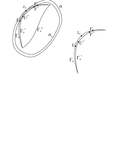
Figure 4:

For a small $a$ let $\sigma_{a}$ be the lemniscate $\sigma_{a}:=\{z\;:\;|T_{N}(z)|=e^{-a}\}$. According to [24, Section 3], if $\Delta\subset\Delta_{0}$ is a fixed small neighborhood of $z_{0}$, then for sufficiently small $a$ this $\sigma_{a}$ contains $\Gamma^{\prime}\setminus\Delta$ in its interior, while in $\Delta$ the two curves $\Gamma_{0}$ and $\sigma_{a}$ intersect in two points $U,V$, see Figure 4. The points $U$ and $V$ are connected by the arc $\overline{UV}_{\Gamma_{0}}$ on $\Gamma_{0}$ and also by the arc $\overline{UV}_{\sigma_{a}}$ on $\sigma_{a}$ (there are actually two such arcs on $\sigma_{a}$, we take the one lying in $\Delta$). For each $\Gamma_{j}$ which is a Jordan arc connect the two endpoints of $\Gamma_{j}$ by a new $C^{2}$ Jordan arc $\Gamma_{j}^{*}$ going inside $\Gamma^{\prime}$ so that on $\Gamma_{j}^{*}$ we have

$$g_{\Omega}(z)\leq a^{2},\qquad z\in\Gamma_{j}^{*}.$$ (7.39)

In addition, $\Gamma_{0}^{*}$ can be selected so that in $\Delta$ it intersects $\sigma_{a}$ in two points $U^{*},V^{*}$. Then $\overline{U^{*}V^{*}}_{\sigma_{a}}$ is a subarc of $\overline{UV}_{\sigma_{a}}$. Let now $\Gamma^{*}$ be the union of $\Gamma$, of the $\Gamma_{j}^{*}$’s with $j>0$, of $\Gamma_{0}^{*}\setminus\overline{U^{*}V^{*}}_{\Gamma_{0}^{*}}$ and of $\overline{U^{*}V^{*}}_{\sigma_{a}}$. This $\Gamma^{*}$ is the union of $k_{0}+1$ piecewise smooth Jordan curves.

Now let

$$m=\left[(1+\varepsilon)^{7}A_{-}n/NA_{+}\right]$$ (7.40)

and consider the polynomial

$$P_{n+mN}(z)=Q_{n}(z)T_{N}(z)^{m}$$ (7.41)

on $\Gamma^{*}$ with the $Q_{n}$ from (7.33), and let the measure $\mu^{*}$ be the measure in (7.34) on $\Gamma^{*}$. For the polynomials $P_{n+Nm}$ it was shown in [24, (3.18)-(3.20)] that on $\Gamma^{*}\setminus\left(\overline{UV}_{\Gamma_{0}}\cup\overline{U^{*}V^{*}}_{\sigma_{a}}\right)$,

$$|P_{n+mN}(z)|\leq C_{1}n^{1/2}e^{na^{2}-ma},$$ (7.42)

on $\overline{UV}_{\Gamma_{0}}$

$$|P_{n+mN}(z)|\leq|Q_{n}(z)|,$$ (7.43)

and on $\overline{U^{*}V^{*}}_{\sigma_{a}}$

$$|P_{n+mN}(z)|\leq C_{1}n^{1/2}\exp\left(n(1+\varepsilon)^{4}aA_{-}/|T_{N}^{\prime}(z_{0})|-ma\right),$$ (7.44)

where $C_{1}$ is a fixed constant. Here, by the choice of $m$ in (7.40), and by (7.37) and (7.38), the last exponent is at most

$$n\left(\frac{(1+\varepsilon)^{5}aA_{-}}{A_{+}N}-\frac{(1+\varepsilon)^{6}aA_{-}}{NA_{+}}\right)=-\varepsilon n\frac{(1+\varepsilon)^{5}aA_{-}}{NA_{+}}.$$

Fix $a$ so small that we have $a^{2}-aA_{-}/NA_{+}<0$. Then the inequality $|T_{N}(z)|\leq 1$ for $z\in\Gamma^{*}$ and the estimates (7.42)–(7.44) yield

$$\lambda_{n+mN}(\mu^{*},z_{0})\leq\int|P_{n+mN}|^{2}d\mu^{*}\leq\int|Q_{n}|^{2}d\mu+O(n^{-\alpha-2}).$$

Hence, by (7.33), for infinitely many $n$

$$(n+mN)^{\alpha+1}\lambda_{n+mN}(\mu^{*},z_{0})\leq\left(\frac{n+mN}{n}\right)^{\alpha+1}\left(1-\delta\right)\frac{w(z_{0})L_{\alpha}}{(\pi\omega_{\Gamma}(z_{0}))^{\alpha+1}}+o(1).$$ (7.45)

Since (see [24, (3.22)–(3.23)])

$$\omega_{\Gamma}(z_{0})=\frac{1}{2\pi}\left(\frac{\partial g_{\Omega}}{\partial{\bf n}_{+}}+\frac{\partial g_{\Omega}}{\partial{\bf n}_{-}}\right)=\frac{1}{2\pi}(A_{+}+A_{-})$$ (7.46)

and

$$\omega_{\Gamma^{*}}(z_{0})=\frac{1}{2\pi}\frac{\partial g_{\Omega^{*}}(z_{0})}{\partial{\bf n}_{+}}\leq\frac{1}{2\pi}\frac{\partial g_{\Omega}(z_{0})}{\partial{\bf n}_{+}}=\frac{1}{2\pi}A_{+},$$ (7.47)

we have

$$\left(\frac{n+mN}{n}\right)^{\alpha+1}\left(1-\delta\right) \hskip-15.0pt\frac{w(z_{0})L_{\alpha}}{(\pi\omega_{\Gamma}(z_{0}))^{\alpha+1}}\leq\left(1+(1+\varepsilon)^{7}\frac{A_{-}}{A_{+}}\right)^{\alpha+1}\times$$

$$\hskip-28.45274pt\left(1-\delta\right)\frac{w(z_{0})L_{\alpha}}{(\pi\omega_{\Gamma^{*}}(z_{0}))^{\alpha+1}}\left(\frac{A_{+}}{A_{+}+A_{-}}\right)^{\alpha+1}$$

$$\leq\left(1-\frac{\delta}{2}\right)\frac{w(z_{0})L_{\alpha}}{(\pi\omega_{\Gamma^{*}}(z_{0}))^{\alpha+1}}$$

if $\varepsilon$ is sufficiently small. Therefore, (7.45) implies

$$\liminf_{n\to\infty}(n+mN)^{\alpha+1}\lambda_{n+mN}(\mu^{*},z_{0})\leq\left(1-\frac{\delta}{2}\right)\frac{w(z_{0})L_{\alpha}}{(\pi\omega_{\Gamma^{*}}(z_{0}))^{\alpha+1}},$$

which is impossible according to Proposition 6.1. This contradiction shows that (7.33) is impossible, and so

$$\liminf_{n\to\infty}n\lambda_{n}(\mu,z_{0})\geq\frac{w(z_{0})L_{\alpha}}{(\pi\omega_{\Gamma}(z_{0}))^{\alpha+1}}.$$ (7.48)

follows.  

(7.30) and (7.48) prove Proposition 7.1.

8 Proof of Theorem 1.1

Let $\Gamma$ be as in the theorem, and let $\Gamma=\cup_{k=0}^{k_{0}}\Gamma^{k}$ be the connected components of $\Gamma$. Let $\Omega$ be the unbounded connected component of $\overline{\mathbb{C}}\setminus\Gamma$. We may assume that $z_{0}\in\Gamma_{0}$. By assumption, $z_{0}$ lies on a $C^{2}$-smooth arc $J$ of $\partial\Omega$, and there is an open set $O$ such that $J=\Gamma\cap O$. Let $\Delta_{\delta}(z_{0})$ be a small disk about $z_{0}$ that lies in $O$ together with its closure. Now there are two possibilities for $J$:

Type I

only one side of $J$ belongs to $\Omega$,

Type II

both sides of $J$ belong to $\Omega$.

Type I occurs when $\Gamma^{0}\setminus\Delta_{\delta}(z_{0})$ is connected, and Type II occurs when this is not the case.

Let $g_{\Omega}(z)$ be the Green’s function for the domain $\Omega$ with pole at infinity, which we assume to be defined to be 0 outside $\Omega$. The proof of Theorem 1.1 is based on the following propositions.

Proposition 8.1

If $J$ is of Type I, then there is a sequence $\{\Gamma_{m}\}$ of sets consisting of disjoint $C^{2}$-smooth Jordan curves $\Gamma_{m}^{k}$, $k=0,1,\ldots,k_{0}$, such that with some positive sequence $\{\varepsilon_{m}\}$ tending to 0 we have

(i)

$z_{0}\in\Gamma_{m}^{0}$ and $\Gamma\cap\overline{\Delta_{\delta}(z_{0})}=\Gamma_{m}\cap\overline{\Delta_{\delta}(z_{0})}$,

(ii)

$$\frac{1}{1+\varepsilon_{m}}\omega_{\Gamma}(z_{0})\leq\omega_{\Gamma_{m}}(z_{0})\leq(1+\varepsilon_{m})\omega_{\Gamma}(z_{0}),$$

(iii)

$$\max_{x\in\Gamma_{m}}g_{\Omega}(z)\leq\varepsilon_{m},\qquad\max_{x\in\Gamma}g_{\Omega_{m}}(z)\leq\varepsilon_{m}.$$

(iv)

The Hausdorff distance of the outer boundaries of $\Gamma$ and $\Gamma_{m}$ tends to 0 as $m\to\infty$.

Property (i) means that in the $\delta$-neighborhood of $z_{0}$ the sets $\Gamma_{m}$ and $\Gamma$ coincide.

Proposition 8.2

If $J$ is of Type II, then there is a sequence $\{\Gamma_{m}\}$ of sets consisting of $\Gamma_{m}^{0}:=J\cap\overline{\Delta_{\delta}(z_{0})}$ and of disjoint $C^{2}$ Jordan curves $\Gamma_{m}^{k}$, $k=1,\ldots,k_{0}+2$, lying in the component of $\Gamma_{m}^{0}$ such that (i)–(iv) above hold.

Pending the proofs of these propositions now we complete the proof of Theorem 1.1. It follows from (i) and (iv) that there is a compact set $K$ that contains $\Gamma$ and all $\Gamma_{m}$ such that $z_{0}$ lies on the outer boundary of $K$, and in a neighborhood of $z_{0}$ the outer boundary of $K$ and $\Gamma$ are the same. In particular, there is a circle in the unbounded component of $\overline{\mathbb{C}}\setminus K$ that contains $z_{0}$ on its boundary, so we can apply Proposition 2.1 to $K$ and $z_{0}$.

Fix an $m$ and consider the set $\Gamma_{m}$ either from Proposition 8.1 if $J$ is of Type I or from Proposition 8.2 if $J$ is of Type II. We define the measure

$$\mu_{m}(z)=w(z)|z-z_{0}|^{\alpha}ds_{\Gamma_{m}}(z),$$

where $w$ is a continuous and positive extension of the original $w$ (that existed on $J$) from $J\cap\overline{\Delta_{\delta}(z_{0})}$ to $\Gamma_{m}$. It follows from the Erdős-Turán criterion [19, Theorem 4.1.1] that this $\mu_{m}$ is in the ${\bf Reg}$ class.

For positive integer $n$ let $P_{n}$ be the extremal polynomial of degree $n$ for $\lambda_{n}(\mu,z)$. Consider the polynomial $S_{4n\varepsilon_{m}/c_{2}\delta^{2},z_{0},K}(z)$ from Proposition 2.1 with $\gamma=2$ (here $c_{2}$ is the constant from Proposition 2.1), and form the product $Q_{n}(z)=P_{n}(z)S_{4n\varepsilon_{m}/c_{2}\delta^{2},z_{0},K}(z)$. This is a polynomial of degree at most $n(1+4\varepsilon_{m}/c_{2}\delta^{2})$ which takes the value 1 at $z_{0}$. On $\Gamma_{m}\cap\overline{\Delta_{\delta}(z_{0})}=\Gamma\cap\overline{\Delta_{\delta}(z_{0})}$ we have

$$\int_{\Gamma_{m}\cap\overline{\Delta_{\delta}(z_{0})}}|Q_{n}(z)|^{2}\leq\int_{\Gamma\cap\overline{\Delta_{\delta}(z_{0})}}|P_{n}(z)|^{2}\leq\lambda_{n}(\mu,z_{0}).$$ (8.1)

Since the $L^{2}(\mu)$-norms of $\{P_{n}\}$ are bounded, it follows from $\mu\in{\bf Reg}$ that there is an $n_{m}$ such that if $n\geq n_{m}$, then we have

$$\|P_{n}\|_{\Gamma}\leq e^{\varepsilon_{m}n}.$$

Then, by the Bernstein-Walsh lemma (Lemma 2.10) and by property (iii), we have for all $z\in\Gamma_{m}$

$$|P_{n}(z)|\leq\|P_{n}\|_{\Gamma}e^{ng_{\Omega}(z)}\leq e^{2n\varepsilon_{m}}.$$

Therefore, (2.3) and $\Gamma_{m}\subseteq K$ imply that for $z\in\Gamma_{m}\setminus\overline{\Delta_{\delta}(z_{0})}$

$$|Q_{n}(z)|\leq\exp(2n\varepsilon_{m}-[4n\varepsilon_{m}/c_{2}\delta^{2}]c_{2}\delta^{2})<e^{-n\varepsilon_{m}}$$

if $n$ is sufficiently large. As a consequence, the integral of $Q_{n}$ over $\Gamma_{m}\setminus\overline{\Delta_{\delta}(z_{0})}$ is exponentially small in $n$, which, combined with (8.1), yields that

$$\lambda_{n(1+4\varepsilon_{m}/c_{2}\delta^{2})}(\mu_{m},z_{0})\leq\lambda_{n}(\mu,z_{0})+o(n^{-(1+\alpha)}).$$

Multiply here both sides by $n(1+4\varepsilon_{m}/c_{2}\delta^{2})^{1+\alpha}$ and let $n$ tend to infinity. If we apply that Theorem 1.1 has already been proven for $\Gamma_{m}$ and for the measure $\mu_{m}$ (see Proposition 7.1), we can conclude (use also (2.1))

$$\liminf_{n\to\infty}n^{\alpha+1}\lambda_{n}(\mu,z_{0})\geq\frac{1}{1+4\varepsilon_{m}/c_{2}\delta^{2}}\frac{w(z_{0})}{(\pi\omega_{\Gamma_{m}}(z_{0}))^{\alpha+1}}L_{\alpha}$$

(with the $L_{\alpha}$ from (3.4)), and an application of property (ii) yields then

$$\liminf_{n\to\infty}n^{\alpha+1}\lambda_{n}(\mu,z_{0})\geq\frac{1}{(1+\varepsilon_{m})^{|\alpha|+1}(1+4\varepsilon_{m}/c_{2}\delta^{2})}\frac{w(z_{0})}{(\pi\omega_{\Gamma}(z_{0}))^{\alpha+1}}L_{\alpha}.$$

If we reverse the roles of $\Gamma$ and $\Gamma_{m}$ in this argument, then we can similarly conclude

$$\limsup_{n\to\infty}n^{\alpha+1}\lambda_{n}(\mu,z_{0})\leq(1+\varepsilon_{m})^{|\alpha|+1}(1+4\varepsilon_{m}/c_{2}\delta^{2})\frac{w(z_{0})}{(\pi\omega_{\Gamma}(z_{0}))^{2}}L_{\alpha}.$$

Finally, in these last two relations we can let $m\to\infty$, and as $\varepsilon_{m}\to 0$, the limit in Theorem 1.1 follows.

Thus, it is left to prove Propositions 8.1 and 8.2.

8.1 Proof of Proposition 8.1

Both in this proof and in the next one we shall use that if $\Omega_{1}\subset\Omega_{2}$ (say both with a smooth boundary), and $z\in\Omega_{1}$, then $g_{\Omega_{1}}(z)\leq g_{\Omega_{2}}(z)$. As a consequence, if $z$ is a common point on their boundaries, then the normal derivative of $g_{\Omega_{1}}$ (the normal pointing inside $\Omega_{1}$) is not larger than the same normal derivative of $g_{\Omega_{2}}$ (because both Green’s functions vanish on the common boundary). Since, modulo a factor $1/2\pi$, the normal derivatives yield the equilibrium densities (see formulae (8.2) and (8.4) below), it also follows that if $\Gamma_{1}\subset\Gamma_{2}$, then on (an arc of) $\Gamma_{1}$ the equilibrium density $\omega_{\Gamma_{2}}$ is at most as least as large as the equilibrium density $\omega_{\Gamma_{1}}$ (see also [17, Theorem IV.1.6(e)], according to which the equilibrium measure for $\Gamma_{1}$ is the balayage onto $\Gamma_{1}$ of the equilibrium measure of $\Gamma_{2}$).

Choose, for each $m$ and $1\leq k\leq k_{0}$, $C^{2}$-smooth Jordan curves $\Gamma_{m}^{k}$ so that they lie in $\Omega$ and are of distance $<1/m$ from $\Gamma^{k}$. For $k=0$ the choice is somewhat different: let $\Gamma_{m}^{0}$ be a $C^{2}$ Jordan curve that lies in $\overline{\Omega}$, its distance from $\Gamma^{0}$ is smaller than $1/m$, $J\cap\overline{\Delta_{\delta}(z_{0})}\subset\Gamma_{m}^{0}$, and $\Gamma_{m}^{0}\setminus J$ lies in $\Omega$, see Figure 5. We can select these so that the outer domains $\Omega_{m}$ of $\Gamma_{m}$ are increasing with $m$. From this construction it is clear that (i) and (iv) are true.

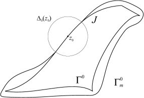
Figure 5: The arc $J$ and the selection of $\Gamma_{m}^{0}$

Now $\overline{\mathbb{C}}\setminus\Omega_{m}$ (the so called polynomial convex hull of $\Gamma_{m}$) is a shrinking sequence of compact sets, the intersection of which is $\overline{\mathbb{C}}\setminus\Omega$. Therefore, if ${\rm cap}$ denotes the logarithmic capacity, then we have (see [16, Theorem 5.1.3]) ${\rm cap}(\overline{\mathbb{C}}\setminus\Omega_{m})\to{\rm cap}(\overline{\mathbb{C}}\setminus\Omega)$. Since $\{g_{\Omega}(z)-g_{\Omega_{m}}(z)\}$ is a decreasing sequence of positive harmonic functions (more precisely, this sequence starting from the term $g_{\Omega}(z)-g_{\Omega_{l}}(z)$ is harmonic in $\Omega_{l}$) for which (see [16, Theorem 5.2.1])

$$g_{\Omega}(\infty)-g_{\Omega_{m}}(\infty)=\log\frac{1}{{\rm cap}(\overline{\mathbb{C}}\setminus\Omega)}-\frac{1}{{\rm cap}(\overline{\mathbb{C}}\setminus\Omega_{m})}\to 0,$$

we obtain from Harnack’s theorem ([16, Theorem 1.3.9]) that $g_{\Omega}(z)-g_{\Omega_{m}}(z)\to 0$ locally uniformly on compact subsets of $\Omega$. This, and the fact that this sequence is defined in $\Omega\cap\Delta_{\delta}(z_{0})$ and has boundary values identically 0 on $\partial\Omega\cap\Delta_{\delta}(z_{0})$, then implies (see e.g. [11, Lemma 7.1]) the following: if ${\bf n}$ denotes the normal to $z_{0}$ in the direction of $\Omega$ then, as $m\to\infty$,

$$\frac{\partial g_{\Omega_{m}}(z_{0})}{\partial{\bf n}}\to\frac{\partial g_{\Omega}(z_{0})}{\partial{\bf n}}.$$

But in the Type I situation we have (see [14, II.(4.1)] combined with [16, Theorem 4.3.14] or [17, Theorem IV.2.3] and [17, (I.4.8)])

$$\omega_{\Gamma}(z_{0})=\frac{1}{2\pi}\frac{\partial g_{\Omega}(z_{0})}{\partial{\bf n}},$$ (8.2)

and a similar formula is true for $\omega_{\Gamma_{m}}$, hence

$$\omega_{\Gamma_{m}}(z_{0})\to\omega_{\Gamma}(z_{0}),\qquad m\to\infty.$$

This takes care of (ii).

Finally, we use the following statement from [22, Theorem 7.1]:

Lemma 8.3

Let $S$ be a continuum. Then the Green’s function $g_{\overline{\mathbb{C}}\setminus S}(z,\infty)$ is uniformly Hölder $1/2$ continuous on $S$, i.e. if $z_{0}\in\Omega$, then

$$g_{\overline{\mathbb{C}}\setminus S}(z_{0},\infty)\leq C{\rm dist}(z_{0},S)^{1/2}.$$ (8.3)

Furthermore, here $C$ can be chosen to depend only on the diameter of $S$.

If we apply this with $S=\Gamma^{k}$, $k=0,\ldots,k_{0}$ and use that $g_{\Omega_{m}}(z)\leq g_{\Omega_{m}^{k}}(z)$ for each $k$ (where, of course, $\Omega_{m}^{k}$ is the unbounded component of $\overline{\mathbb{C}}\setminus\Gamma_{m}^{k}$), then we can conclude the first inequality in (iii). In this case (i.e. when $J$ is of Type I), the second inequality in (iii) is trivial, since, by the construction, $g_{\Omega_{m}}$ is identically 0 on $\Gamma$.  

8.2 Proof of Proposition 8.2

For an $m$ let $J_{1,m}$ resp. $J_{2,m}$ be the two open subarcs of $J$ of diameter $1/m$ that lie outside $\Delta_{\delta}(z_{0})$, but which have one endpoint in $\overline{\Delta_{\delta}(z_{0})}$ (see Figure 6) (for large $m$ these exist).

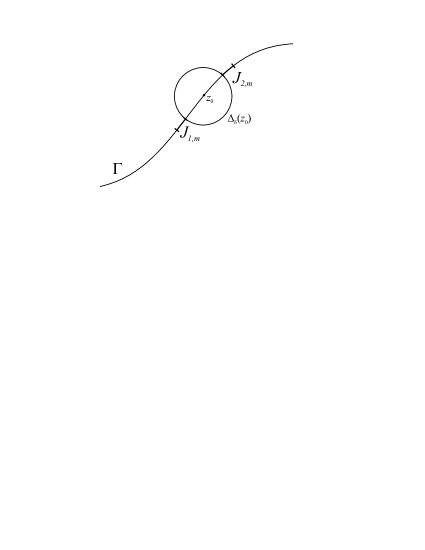
Figure 6: The arcs $J_{1,m}$ and $J_{2,m}$

Remove now $J_{1,m}$ and $J_{2,m}$ from $\Gamma$. Since we are in the Type II situation, after this removal the unbounded component of the complement of $\Gamma^{0}\setminus({J_{1,m}\cup J_{2,m}})$ is $\Omega\cup J_{1,m}\cup J_{2,m}$, and $\Gamma^{0}\setminus(J_{1,m}\cup J_{2,m})$ splits into three connected components, one of them being $J\cap\overline{\Delta_{\delta}(z_{0})}$. Let $\Gamma^{0,1},\Gamma^{0,2}$ be the other two components of $\Gamma^{0}\setminus({J_{1,m}\cup J_{2,m}})$. As $m\to\infty$ we have ${\rm cap}(\overline{\mathbb{C}}\setminus(\Omega\cup{J_{1,m}\cup J_{2,m}}))\to{\rm cap}(\overline{\mathbb{C}}\setminus\Omega)$, and since now the domains $\Omega\cup{J_{1,m}\cup J_{2,m}}$ are shrinking, we can conclude from Harnack’s theorem as before that $g_{\Omega}(z)-g_{\Omega_{m}}(z)\to 0$ locally uniformly on compact subsets of $\Omega$. This implies again that if ${\bf n}_{\pm}$ are the two normals to $\Gamma$ at $z_{0}$ (note that now both point inside $\Omega$), then

$$\frac{\partial g_{\Omega\cup{J_{1,m}\cup J_{2,m}}}(z_{0})}{\partial{\bf n\pm}}\to\frac{\partial g_{\Omega}(z_{0})}{\partial{\bf n}}$$

as $m\to\infty$. Since now (see [14, II.(4.1)] or [17, Theorem IV.2.3] and [17, (I.4.8)])

$$\omega_{\Gamma}(z_{0})=\frac{1}{2\pi}\left(\frac{\partial g_{\Omega}(z_{0})}{\partial{\bf n}_{+}}+\frac{\partial g_{\Omega}(z_{0})}{\partial{\bf n}_{-}}\right),$$ (8.4)

we can conclude again that

$$0\leq\omega_{\Gamma\setminus(J_{1,m}\cup J_{2,m})}(z_{0})-\omega_{\Gamma}(z_{0})<\varepsilon_{m}$$ (8.5)

with some $\varepsilon_{m}>0$ that tends to 0 as $m\to\infty$. By selecting a somewhat larger $\varepsilon_{m}$ we may also assume

$$g_{\Omega\cup{J_{1,m}\cup J_{2,m}}}(z)<\varepsilon_{m},\qquad z\in J_{1,m}\cup J_{2,m}$$ (8.6)

(apply Lemma 8.3 to $S=\Gamma\cap\overline{\Delta_{\delta}(z_{0})}$ and use that $g_{\Omega\cup{J_{1,m}\cup J_{2,m}}}(z)\leq g_{\overline{\mathbb{C}}\setminus(\Gamma\cap\overline{\Delta_{\delta}(z_{0})})}(z)$).

For the continua $\Gamma^{0,1},\Gamma^{0,2},\Gamma_{1},\Gamma_{2},\ldots,\Gamma_{k_{0}}$ and for a small $0<\theta<1/m$ select $C^{2}$-smooth Jordan curves $\gamma^{0,1},\gamma^{0,2},\gamma_{1},\gamma_{2},\ldots,\gamma_{k_{0}}$ that lie in $\Omega\cup{J_{1,m}\cup J_{2,m}}$ and are of distance $<\theta$ from the corresponding continuum. Let $\Gamma_{m,\theta}$ be the union of $J\cap\overline{\Delta_{\delta}(z_{0})}$ and of these last chosen Jordan curves. Then $\Gamma_{m,\theta}$ consists (for small $\theta$) of $k_{0}+2$ Jordan curves and one Jordan arc (namely $J\cap\overline{\Delta_{\delta}(z_{0})}$), all of them $C^{2}$-smooth. According to the proof of Proposition 8.1 we have

$$\omega_{\Gamma_{m,\theta}}(z_{0})\to\omega_{\Gamma\setminus(J_{1,m}\cup J_{2,m})}(z_{0})$$

as $\theta\to 0$, therefore, for sufficiently small $\theta$, we have (see (8.5))

$$-\varepsilon_{m}<\omega_{\Gamma_{m,\theta}}(z_{0})-\omega_{\Gamma}(z_{0})<\varepsilon_{m}.$$

Thus, if $\theta$ is sufficiently small, we have properties (i), (ii) and (iv) in the proposition for $\Gamma_{m}=\Gamma_{m,\theta}$. The first inequality in (iii) follows exactly as at the end of the proof of Proposition 8.1. Finally, the second inequality in (iii) follows from (8.6) because

$$g_{\Omega_{m,\theta}}(z)\leq g_{\Omega\cup{J_{1,m}\cup J_{2,m}}}(z),$$

(where $\Omega_{m,\theta}$ is the unbounded component of $\overline{\mathbb{C}}\setminus\Gamma_{m,\theta}$) and $g_{\Omega_{m,\theta}}(z)=0$ if $z\in\Gamma$ unless $z\in J_{1,m}\cup J_{2,m}$.

These show that for sufficiently small $\theta$ we can select $\Gamma_{m}$ in Proposition 8.2 as $\Gamma_{m,\theta}$.  

9 Proof of Theorem 1.2

Let $\Gamma$ be as in Theorem 1.2, and let $\Gamma=\cup_{k=0}^{k_{0}}\Gamma_{k}$ be the connected components of $\Gamma$, $\Gamma_{0}$ being the one that contains $z_{0}$. We may assume that $z_{0}=0$. Set

$$\tilde{\Gamma}=\{z\;:\;z^{2}\in\Gamma\},\qquad\tilde{\Gamma}_{k}=\{z\;:\;z^{2}\in\Gamma_{k}\}.$$

Every $\tilde{\Gamma}_{k}$ is the union of two disjoint continua: $\tilde{\Gamma}_{k}=\Gamma_{k}^{+}\cup\tilde{\Gamma}_{k}^{-}$, where $\tilde{\Gamma}_{k}^{-}=-\tilde{\Gamma}_{k}^{+}$. Set $\tilde{\Gamma}^{\pm}=\cup_{k}\tilde{\Gamma}_{k}^{\pm}$. All the $\tilde{\Gamma}_{k}^{\pm}$ are disjoint, except when $k=0$: then 0 is a common point of $\Gamma_{0}^{\pm}$, but except for that point, $\tilde{\Gamma}_{0}^{+}$ and $\tilde{\Gamma}_{0}^{-}$ are again disjoint. In general, we shall use the notation $\tilde{H}$ for the set of points $z$ for which $z^{2}$ belongs to $H$, and if $H$ is a continuum, then represent $\tilde{H}$ as the union of two continua $\tilde{H}^{+}\cup\tilde{H}^{-}$, where $\tilde{H}^{-}=-\tilde{H}^{+}$, and $\tilde{H}^{-}$ and $\tilde{H}^{+}$ are disjoint except perhaps for the point 0 if 0 belongs to $H$.

Now $\tilde{\Gamma}_{0}^{+}\cup\tilde{\Gamma}_{0}^{-}$ is connected, and if $J$ is the $C^{2}$-smooth arc of $\Gamma$ with one endpoint at $z_{0}=0$, then $\tilde{J}$ is a $C^{2}$-smooth arc that lies on the outer boundary of $\tilde{\Gamma}$, and $\tilde{J}$ contains 0 in its (one-dimensional) interior. Thus, $\tilde{\Gamma}$ and $z_{0}=0$ satisfy the assumptions in Theorem 1.1.

For a measure $\mu$ defined on $\Gamma$ let $\tilde{\mu}$ be the measure $d\tilde{\mu}(z)=\frac{1}{2}d\mu(z^{2})$, i.e. if, say, $E\subset\tilde{\Gamma}^{+}$ is a Borel set and $E^{2}=\{z^{2}\;:\;z\in E\}$, then

$$\tilde{\mu}(E)=\frac{1}{2}\mu(E^{2}),$$

and a similar formula holds for $E\subset\Gamma^{-}$. So $\tilde{\mu}$ is an even measure, which has the same total mass as $\mu$ has.

Let $\nu_{\Gamma}$ be the equilibrium measure of $\Gamma$. We claim that $\nu_{\tilde{\Gamma}}=\widetilde{\nu_{\Gamma}}.$ Indeed, for any $z\in\tilde{\Gamma}$ we have

$$\int\log|z-t|d\widetilde{\nu_{\Gamma}}(t) = \int_{\tilde{\Gamma}^{+}}(\log|z-t|+\log|z+t|)d\widetilde{\nu_{\Gamma}}(t)$$

$$= \frac{1}{2}\int_{\Gamma}\log|z^{2}-t^{2}|d\nu_{\Gamma}(t^{2})$$

$$= \frac{1}{2}\int\log|z^{2}-u|d\nu_{\Gamma}(u)={\rm const}$$

because the equilibrium potential of $\nu_{\Gamma}$ is constant on $\Gamma$ by Frostman’s theorem (see [16, Theorem 3.3.4]), and $z^{2}\in\Gamma$. Since the equilibrium measure $\nu_{\tilde{\Gamma}}$ is characterized (among all probability measures on $\tilde{\Gamma}$) by the fact that its logarithmic potential is constant on the given set, we can conclude that $\widetilde{\nu_{\Gamma}}$ is, indeed, the equilibrium measure of $\tilde{\Gamma}$ (here we use that all the sets which we are considering are the unions of finitely many continua, hence the equilibrium potentials for them are continuous everywhere).

Let $\gamma(t)$ be a parametrization of $\tilde{J}^{+}$ with $\gamma(0)=0$. Then $\gamma(t)^{2}$ is a parametrization of $J$, and the two corresponding arc measures are $|\gamma^{\prime}(t)|dt$ and $|(\gamma(t)^{2})^{\prime}|dt=2|\gamma(t)||\gamma^{\prime}(t)|dt$, resp. Therefore, since the $\nu_{\tilde{\Gamma}}$-measure of an arc $\{\gamma(t)\;:\;t_{1}\leq t\leq t_{2}\}$ is the same as half of the $\nu_{\Gamma}$-measure of the arc $\{\gamma(t)^{2}\;:\;t_{1}\leq t\leq t_{2}\}$, we have

$$\int_{t_{1}}^{t_{2}}\omega_{\tilde{\Gamma}}(\gamma(t))|\gamma^{\prime}(t)|dt=\frac{1}{2}\int_{t_{1}}^{t_{2}}\omega_{\Gamma}(\gamma(t)^{2})2|\gamma(t)||\gamma^{\prime}(t)|dt,$$

from which

$$\omega_{\tilde{\Gamma}}(\gamma(t))=\omega_{\Gamma}(\gamma(t)^{2})|\gamma(t)|,\qquad t\in\tilde{J}^{+},$$

follows (recall, that on both sides the $\omega$ is the equilibrium density with respect to the corresponding arc measure). A similar formula holds on $\tilde{J}^{-}$. But $\omega_{\tilde{\Gamma}}(z)$ is continuous and positive at $0$ (see e.g. [24, Proposition 2.2]), therefore the preceding formula shows that $\omega_{\Gamma}(z)$ behaves around 0 as $\omega_{\tilde{\Gamma}}(0)/\sqrt{|z|}$, and we have (see (1.5) for the definition of $M(\Gamma,0)$)

$$M(\Gamma,0)=\lim_{z\to 0}\sqrt{|z|}\omega_{\Gamma}(z)=\omega_{\tilde{\Gamma}}(0).$$ (9.1)

Now the same argument that was used in the proof of Proposition 3.2 (see in particular (3.6)) shows that

$$\lambda_{2n}(\tilde{\mu},0)=\lambda_{n}(\mu,0).$$ (9.2)

$\mu$ was assumed to be of the form $w(z)|z|^{\alpha}ds_{J}(z)$ on $J$, hence, as before,

$$\int_{t_{1}}^{t_{2}}d\tilde{\mu}(t)=\frac{1}{2}\int_{t_{1}}^{t_{2}}w(\gamma(t)^{2})|\gamma(t)^{2}|^{\alpha}2|\gamma(t)||\gamma^{\prime}(t)|dt,$$

and since here $|\gamma^{\prime}(t)|dt$ is the arc measure on $\tilde{J}^{+}$, we can conclude that on $\tilde{J}^{+}$ the measure $\tilde{\mu}$ has the form $d\tilde{\mu}(z)=w(z^{2})|z|^{2\alpha+1}ds_{\tilde{J}}(z)$, and the same representation holds on $\tilde{J}^{-}$. Therefore, Theorem 1.1 can be applied to the set $\tilde{\Gamma}$, to the measure $\tilde{\mu}$ and to the point $z_{0}=0$, the only change is that now $\alpha$ has to be replaced by $2\alpha+1$ when dealing with the measure $\tilde{\mu}$. Now we obtain from (9.2)

$$\lim_{n\to\infty}(2n)^{2\alpha+2}\lambda_{2n}(\tilde{\mu},0)=\lim_{n\to\infty}(2n)^{2\alpha+2}\lambda_{n}(\mu,0),$$

and since, according to Theorem 1.1, the limit on the left is

$$2^{2\alpha+2}\Gamma\Big{(}\frac{2\alpha+2}{2}\Big{)}\Gamma\Big{(}\frac{2\alpha+4}{2}\Big{)}\frac{w(0)}{(\pi\omega_{\tilde{\Gamma}}(0))^{2\alpha+2}},$$

we obtain

$$\lim_{n\to\infty}n^{2\alpha+2}\lambda_{n}(\mu,0)=\Gamma\Big{(}\alpha+1\Big{)}\Gamma\Big{(}\alpha+2\Big{)}\frac{w(0)}{(\pi\omega_{\tilde{\Gamma}}(0))^{2\alpha+2}},$$

which, in view of (9.1), is the same as (1.6) in Theorem 1.2.  

Vilmos Totik

Bolyai Institute

MTA-SZTE Analysis and Stochastics Research Group

University of Szeged

Szeged

Aradi v. tere 1, 6720, Hungary

and

Department of Mathematics and Statistics

University of South Florida

4202 E. Fowler Ave, CMC342

Tampa, FL 33620-5700, USA

totik@mail.usf.edu

Tivadar Danka

Potential Analysis Research Group, ERC Advanced Grant No. 267055

Bolyai Institute

University of Szeged

Szeged

Aradi v. tere 1, 6720, Hungary

tivadar.danka@math.u-szeged.hu

References

- [1] A. Avila, Y. Last and B. Simon, Bulk universality and clock spacing of zeros for ergodic Jacobi matrices with absolutely continuous spectrum, Anal. PDE, 3(2010), 81 -108.
- [2] D. H. Armitage and S. J. Gardiner, Classical Potential Theory, Springer Verlag, Berlin, Heidelberg, New York, 2002.
- [3] J. B. Garnett and D. E. Marshall, Harmonic measure, New Mathematical Monographs 2, Cambridge University Press, Cambridge, 2008.
- [4] L. Golinskii, The Christoffel function for orthogonal polynomials on a circular arc, J. Approx. Theory, 101(1999), 165–174.
- [5] U. Grenander and G. Szegő, Toeplitz Forms and Their Applications, University of California Press, Berkeley and Los Angeles, 1958.
- [6] B. Gustafsson, M. Putinar, E. Saff, and N. Stylianopoulos, Bergman polynomials on an archipelago: Estimates, zeros and shape reconstruction, Advances in Math., 222(2009), 1405–1460.
- [7] A.B. Kuijlaars and M. Vanlessen, Universality for Eigenvalue Correlations from the Modified Jacobi Unitary Ensemble, Int. Math. Res. Not. IMRN, 30(2002), 1575–1600.
- [8] D. S. Lubinsky, A new approach to universality involving orthogonal polynomials, Annals of Math. 170(2009), 915–939.
- [9] D. S. Lubinsky, A new approach to universality limits at the edge of the spectrum, Integrable systems and random matrices, 281 -290, Contemp. Math., 458, Amer. Math. Soc., Providence, RI, 2008.
- [10] D. S. Lubinsky, Universality limits at the hard edge of the spectrum for measures with compact support, Int. Math. Res. Not. IMRN, 2008, Art. ID rnn 099, 39 pp.
- [11] B. Nagy and V. Totik, Sharpening of Hilbert’s lemniscate theorem, J. D’Analyse Math., Volume 1(2008), 191–223
- [12] P. Nevai, Orthogonal Polynomials, Memoirs of the AMS, no. 213, (1979).
- [13] P. Nevai, Géza Freud, orthogonal polynomials and Christoffel functions. A case study, J. Approx. Theory, 48(1986), 1–167.
- [14] R. Nevanlinna, Analytic Functions, Grundlehren der mathematischen Wissenschaften, 162, Springer Verlag, Berlin, 1970.
- [15] Ch. Pommerenke, On the derivative of a polynomial, Michigan Math. J., 6(1959), 373–375.
- [16] T. Ransford, Potential Theory in the Complex plane, Cambridge University Press, Cambridge, 1995
- [17] E. B. Saff and V. Totik, Logarithmic potentials with external fields, Grundlehren der mathematischen Wissenschaften, 316, Springer Verlag, Berlin, 1997.
- [18] B. Simon, The Christoffel-Darboux kernel, ”Perspectives in PDE, Harmonic Analysis and Applications,” a volume in honor of V.G. Maz’ya’s 70th birthday, Proceedings of Symposia in Pure Mathematics, 79(2008), 295–335.
- [19] H. Stahl and V. Totik, General Orthogonal Polynomials, Encyclopedia of Mathematics and its Applications, 43, Cambridge University Press, Cambridge, 1992.
- [20] G. Szegő, Orthogonal Polynomials, American Mathematical Society Colloquium Publications, American Mathematical Society, Providence, 1975.
- [21] G. Szegő, Collected Papers, ed. R. Askey, Birkhaüser, Boston–Basel–Stuttgart, 1982.
- [22] V. Totik, Christoffel functions on curves and domains, Transactions of the American Mathematical Society, Vol. 362, Number 4, April 2010, 2053–2087.
- [23] V. Totik, The polynomial inverse image method, Approximation Theory XIII: San Antonio 2010, Springer Proceedings in Mathematics, M. Neamtu and L. Schumaker, 345–367.
- [24] V. Totik, Asymptotics of Christoffel functions on arcs and curves, Advances in Mathematics, 252(2014), 114–149.
- [25] V. Totik, Szegő’s problem on curves, American J. Math., 135(2013), 1507–1524.
- [26] T. Varga, Christoffel functions for doubling measures on quasismooth curves and arcs, Acta Math Hungar., 141(2013), 161–184
- [27] J. L. Walsh, Interpolation and Approximation by Rational Functions in the Complex Domain, third edition, Amer. Math. Soc. Colloquium Publications, XX, Amer. Math. Soc., Providence, 1960.
- [28] G. N. Watson, A treatise on the theory of Bessel functions. Reprint of the second (1944) edition. Cambridge University Press, Cambridge, 1995.