Abundance of mode-locking for quasiperiodically forced circle maps

Abstract

We study the phenomenon of mode-locking in the context of quasiperiodically forced non-linear circle maps. As a main result, we show that under certain $\mathcal{C}^{1}$-open condition on the geometry of twist parameter families of such systems, the closure of the union of mode-locking plateaus has positive measure. In particular, this implies the existence of infinitely many mode-locking plateaus (open Arnold tongues). The proof builds on multiscale analysis and parameter exclusion methods in the spirit of Benedicks and Carleson, which were previously developed for quasiperiodic $\textrm{SL}(2,\mathbb{R})$-cocycles by Young and Bjerklöv. The methods apply to a variety of examples, including a forced version of the classical Arnold circle map.

1 Introduction

The paradigm example for the phenomenon of mode-locking in dynamical systems is the Arnold circle map

(1.1) $$f_{\alpha,\tau}:\mathbb{T}^{1}\to\mathbb{T}^{1}\quad,\quad x\mapsto x+\tau+\frac{\alpha}{2\pi}\sin(2\pi x)\ \bmod 1\ ,$$

with non-linearity parameter $\alpha\in[0,1]$ and twist parameter $\tau\in[0,1]$. If $F_{\alpha,\tau}:\mathbb{R}\to\mathbb{R}$ denotes the canonical lift of $f_{\alpha,\tau}$, then its rotation number is given by

(1.2) $$\rho(F_{\alpha,\tau})\ =\ \lim_{n\rightarrow\infty}(F_{\alpha,\tau}^{n}(x)-x)/n\ .$$

Mode-locking in this context refers to the fact that for certain values of $\alpha$ and $\tau$ the mapping $\tau^{\prime}\mapsto\rho(F_{\alpha,\tau^{\prime}})$ is locally constant in $\tau^{\prime}=\tau$. Maximal parameter intervals with constant rotation number are called mode-locking plateaus. It is well-known that for the Arnold circle map and similar parameter families mode-locking is abundant. More precisely, for all $\alpha\in(0,1]$ the graph of $[0,1]\to[0,1],\ \tau\mapsto\rho(F_{\alpha,\tau})$ is a devils staircase, that is, it is locally constant on an open and dense subset while increasing from $0$ to $1$ over the unit interval (e.g. [1, Chapter 11]). As a basic model, this gives an understanding of mode-locking phenomena occuring in a variety of real-world situations, including damped pendula and electronic oscillators [2], heart-beat [3] or paradoxical neural behaviour [4, 5].

Generalisations of these results to more complex situations and higher dimension are certainly highly desirable. However, it turns out that substantial difficulties have to be overcome in this direction. One particular example that demonstrates well this fact is the so-called Harper map. It is the real-projective action of a quasiperiodic $\textrm{SL}(2,\mathbb{R})$-cocycle associated to the almost-Mathieu operator, a discrete 1D Schrödinger operator with quasiperiodic potential [6, 7, 8]. Due to an intimate relation between orbits of the Harper map and formal eigenfunctions of the almost-Mathieu operator, a fruitful blend of methods from spectral theory, harmonic analysis and dynamical systems can be used to analyse this model. Nevertheless, it has taken decades before the existence of a devil’s staircase had been established for all parameters in several steps [9, 10, 11].

Here, our aim is to show abundance of mode-locking, in a slightly weaker sense than above, for more general, non-linear quasiperiodically forced (qpf) circle diffeomorphisms. These are skew product diffeomorphisms of the form

(1.3) $$f:\mathbb{T}^{2}\to\mathbb{T}^{2}\quad,\quad(\theta,x)\mapsto(\theta+\omega,f_{\theta}(x))\ ,$$

where $\omega\in\mathbb{R}\setminus\mathbb{Q}$ and all fibre maps $f_{\theta}:\mathbb{T}^{1}\to\mathbb{T}^{1}$ are circle diffeomorphisms. In addition, we require $f$ to be homotopic to the identity and denote the class of such maps by $\mathcal{F}_{\omega}$, where $\omega$ refers to the rotation number on the base. The Harper map mentioned above fits into this setting, although the particular linear-projective structure makes it quite special. In the genuinely non-linear case, much fewer techniques are available for the investigation of such systems, and the theory is far less developed in general.

Yet, there is one well-established method of choice for the analysis of qpf circle diffeomorphisms in the hyperbolic regime – characterised by non-vanishing Lyapunov exponents – which is multiscale analysis and parameter exclusion in the spirit of Benedicks and Carleson [12]. In the above context, it was first developed by Young [13] and Bjerklöv [14, 15] for the linear-projective case and later adapted to non-linear systems in [16, 17]. Originally, this method was used to show the non-uniform hyperbolicity of certain quasiperiodic $\textrm{SL}(2,\mathbb{R})$-cocycles [13, 14], which corresponds to the existence of strange non-chaotic attractors in the general case.

The principle goal of the present article is to develop this approach further, and to show how it can be applied to the problem of mode-locking. The trick which does this is a somewhat twisted argument. In a first step, parameter exclusion is used to identity a large set of parameters for which the dynamics are non-uniformly hyperbolic and minimal and no mode-locking occurs. These are ‘good’ parameters in the sense of the multiscale analysis scheme. In a second step, the information obtained in this process is then used to show that a small shift allows to change from any of these good parameters to a ‘bad’ one, previously excluded during the parameter elimination, at which the multiscale analysis scheme terminates at a finite level and the system becomes uniformly hyperbolic and mode-locked. As a result, this yields that a large set (in the sense of positive Lebesgue measure) of parameters with non-uniformly hyperbolic behaviour can be approximated with mode-locked parameters.

In order to formulate our main result, we denote by $\mathcal{P}_{\omega}$ the set of $\mathcal{C}^{1}$-parameter families of qpf circle diffeomorphisms with parameter $\tau\in\mathbb{T}^{1}$ and rotation number $\omega$ on the base, that is

(1.4) $$\mathcal{P}_{\omega}\ =\ \left\{(f_{\tau})_{\tau\in\mathbb{T}^{1}}\mid f_{\tau}\in\mathcal{F}_{\omega}\ \textrm{ for all }\tau\in\mathbb{T}^{1}\textrm{ and }(\tau,\theta,x)\mapsto f_{\tau}(\theta,x)\textrm{ is }\mathcal{C}^{1}\right\}\ .$$

Elements of $\mathcal{P}_{\omega}$ will be denoted by $\hat{f}$, that is, $\hat{f}=(f_{\tau})_{\tau\in\mathbb{T}^{1}}$. Any $f\in\mathcal{F}_{\omega}$ lifts to a diffeomorphism $F$ of $\mathbb{A}=\mathbb{T}^{1}\times\mathbb{R}$ of the form $F(\theta,x)=(\theta+\omega,F_{\theta}(x))$, where each fibre map $F_{\theta}:\mathbb{R}\to\mathbb{R}$ is a lift of the circle diffeomorphism $f_{\theta}$. The fibred rotation number of $f$ is defined by

(1.5) $$\rho(f)\ =\ \lim_{n\rightarrow\infty}\left(F_{\theta}^{n}(x)-x\right)/n\ \bmod 1\ ,$$

where $F_{\theta}^{n}=F_{\theta+(n-1)\omega}\circ\ldots\circ F_{\theta}$. This limit always exists and is independent of $\theta$ and $x$ [6, 7]. Given $\hat{f}\in\mathcal{P}_{\omega}$, we let

(1.6) $$\mathcal{M}(\hat{f})\ =\ \left\{\tau\in\mathbb{T}^{1}\mid\tau^{\prime}\mapsto\rho(f_{\tau^{\prime}})\textrm{ is locally constant in }\tau^{\prime}=\tau\right\}\ .$$

In other words, $\mathcal{M}(\hat{f})$ is the union of mode-locking plateaus of $\hat{f}$. It is known that on the set $\mathcal{M}(\hat{f})$ the rotation number only takes values in the module $\mathbb{Q}+\omega\mathbb{Q}$ [18].

An $f$-invariant graph is the graph of a measurable function $\varphi:\mathbb{T}^{1}\to\mathbb{T}^{1}$ which satisfies

(1.7) $$f_{\theta}(\varphi(\theta))\ =\ \varphi(\theta+\omega)\ .$$

Hereby, we will identify invariant graphs which coincide Lebesgue-almost surely and implicitly speak of equivalence classes. The (vertical) Lyapunov exponent of an invariant graph is given by

(1.8) $$\lambda(\varphi)\ =\ \int_{\mathbb{T}^{1}}\log\left|f^{\prime}_{\theta}(\varphi(\theta))\right|\ d\theta\ .$$

If an invariant graph is non-continuous, meaning that there is no continuous representative in the equivalence class, and has negative Lyapunov exponent, then it is called a strange non-chaotic attractor (SNA) [19, 20].

Theorem 1.1.

Suppose $\omega$ is Diophantine and $\delta>0$. Then there exists a $\mathcal{C}^{1}$-open set $\mathcal{U}=\mathcal{U}(\omega,\delta)\subseteq\mathcal{P}_{\omega}$ such that for all $(f_{\tau})_{\tau\in\mathbb{T}^{1}}\in\mathcal{U}$ there is a set $\Lambda^{\hat{f}}\subseteq\mathbb{T}^{1}$ of Lebesgue measure $\geq 1-\delta$ with the properties that

• for all $\tau\in\Lambda^{\hat{f}}$, the map $f_{\tau}$ has a (unique) SNA and the dynamics of $f_{\tau}$ are minimal;

• $\Lambda^{\hat{f}}\subseteq\partial\mathcal{M}(\hat{f})$.

For a suitable $\mathcal{C}^{1}$-open set $\mathcal{U}\subseteq\mathcal{P}_{\omega}$, the existence of a set $\Lambda^{\hat{f}}$ with property (i) has already been established in [21]. Hence, the crucial point here is to show that this set from [21] is contained in the boundary of the union of mode-locking plateaus. The proof is based on the above-mentioned multiscale analysis scheme from [13, 14, 16].

We note that (ii) implies the existence of infinitely many open mode-locking plateaus. Yet, at the same time these only take a very small proportion of the parameter space, since the set $\Lambda^{\hat{f}}$ already accounts for measure $1-\delta$. This agrees with the fact that an apparent ‘vanishing’ of the mode-locking plateaus, coming along with the occurrence of SNA, has been reported in numerical studies [22, 23]. (However, it must be emphasized that it was left open by the authors whether or not this observation is a numerical artifact.) The explanation prompted by Theorem 1.1 is that the majority of mode-locking plateaus persist, but simply become too small to be detected numerically. The collapse of single plateaus has been described in [16], in contrast to the situation for the unforced Arnold circle map.

The main aim of the present work is to show how multiscale analysis methods can be applied to mode-locking problems in the non-linear setting. We believe that it is possible to go further in this direction and to combine the presented arguments with recent work by Bjerklöv [24], who extends the multiscale analysis of [14, 15] to all parameters, in order to prove the existence of a devil’s staircase under similar conditions as above. For the special case of quasiperiodic Schrödinger cocycles with $\mathcal{C}^{2}$-potential, such a result has been announced recently by Wang and Zhang [25, 26]. In this setting, however, results on mode-locking have also been established earlier by different methods (Ten Martini Problem, [9, 10, 11]).

The set $\mathcal{U}$ in Theorem 1.1 is characterised explicitely by a number of $\mathcal{C}^{1}$-estimates, which are stated in Section 3. This is important in the context of applications, since it allows to check whether a given parameter family belongs to the set $\mathcal{U}$ or not. Thus, it can be shown that the assertions of the theorem hold for specific examples.

Examples 1.2.

• First, the above statement can easily be applied to parameter families of additively forced circle diffeomorphisms of the form

  (1.9) $$f_{\tau}(\theta,x)\ =\ (\theta+\omega,h(x)+\tau+V(\theta))\ ,$$

  provided the circle diffeomorphism $h:\mathbb{T}^{1}\to\mathbb{T}^{1}$ and the forcing function $V:\mathbb{T}^{1}\to\mathbb{T}^{1}$ have suitable geometric properties. In order to give some explicit examples, suppose $p\geq 2$, let $a_{p}(x)=\int_{0}^{x}1/(1+|\xi|^{p})\ d\xi$ and

  $$h_{\alpha}(x)\ =\ \pi\left(\frac{a_{p}(\alpha\iota(x))}{2a_{p}(\alpha/2)}\right)\$$

  where $\alpha\geq 1$, $\iota:\mathbb{T}^{1}\to(-1/2,1/2]$ is the lift of the identity map on $\mathbb{T}^{1}$ and $\pi:(-1/2,1/2]\to\mathbb{T}^{1}$ is the canonical projection. Further, assume that $V$ is such that for all but finitely many $x\in\mathbb{T}^{1}$ the set $V^{-1}(\{x\})$ consists of exactly two points $\theta_{1}$ and $\theta_{2}$ and we have $V^{\prime}(\theta_{1})<0$ and $V^{\prime}(\theta_{2})>0$. Note that for $p=2$ we have $a_{p}(x)=\arctan(x)$, and $V(\theta)=\cos(2\pi\theta)$ is a possible choice of $V$. In this case, $f_{\tau}$ is the projective action of the quasiperiodic $\textrm{SL}(2,\mathbb{R})$-cocycle $(\theta,v)\mapsto(\theta+\omega,A(\theta)\cdot v)$ with $A(\theta)=R_{V(\theta)+\tau}\cdot\left(\begin{array}[]{cc}\alpha^{1/2}&0\\ 0&\alpha^{-1/2}\end{array}\right)$, where $R_{\vartheta}$ is the rotation matrix with angle $\vartheta$. Yet, for other values of $p$ no such cocycle representation is available.

  If $\omega$ is Diophantine and $\alpha$ is chosen sufficiently large, then the parameter family $f_{\tau}(\theta,x)=(\theta+\omega,h_{\alpha}(x)+\tau+V(\theta)$ belongs to the set $\mathcal{U}$ in Theorem 1.1, which will be explicitely characterised in Section 3 below. The details are easy to check, see [16, Section 3.8] (compare also [21, Corollary 1.2]). Thus, in this case $(f_{\tau})_{\tau\in\mathbb{T}^{1}}$ satisfies the assertions of Theorem 1.1.

• The presented methods and results can also be applied to the quasiperiodically forced version of the Arnold circle map given in (1.1), with a suitable forcing function like $V_{\beta}(\theta)=\arctan(\beta\sin(2\pi\theta))\pi$ with large $\beta>0$. Strictly speaking, some modifications are needed to include this case. This results from the fact that the Arnold circle map does not show arbitrarily strong expansion, which we work with in our proofs below. However, this can be made up for by requiring a special shape of the forcing function, translating into a largeness assumption on $\beta$ above.

  The required modifications have been carried out in detail in [16, 21], and it is on the level of an advanced exercise to implement them as well for our setting. As a result, one obtains that in the parameter family $f_{\tau}(\theta,x)=(\theta+\omega,h_{\alpha,\tau}(x)+V_{\beta}(\theta))$ the boundary of $\mathcal{M}(\hat{f})$ has positive measure, provided $\omega$ is Diophantine, $\alpha\in(0,1)$ and $\beta>0$ is sufficiently large. We note that due to the different geometry, the measure of $\partial\mathcal{M}(\hat{f})$ cannot be ensured to be close to $1$ in this case (compare [16]).

• The most prominent example of a quasiperiodically forced system is probably the so-called Harper map, which is induced real-projective action of the quasiperiodic Schrödinger cocycle associated to the almost-Mathieu operator. It takes the form

  $$f_{\tau}(\theta,x)\ =\ \left(\theta+\omega,\frac{1}{\pi}\arctan\left(\frac{-1}{\tan(\pi x)-\tau+\lambda\cos(2\pi\theta)}\right)\bmod 1\right)\ .$$

  Again, a slight modification of our methods would allow to treat this example for large coupling parameters $\lambda>0$. However, as mentioned above, stronger results are available for this special case [11, 26], so we refrain from providing any details.

Acknowledgements. JW has been supported by a research fellowship of the Alexander-Humboldt-Foundation. TJ has received support of the German Research Council (Emmy-Noether grant Ja 1721/2-1 and Heisenberg-Fellowship Oe 538/7-1). The first ideas for this project have been developed during the International conference on Hamiltonian dynamcs, Nanjing 2011, and the authors would like to thank the organisers for creating the opportunity and Hakan Eliasson for a helpful discussion.

2 Review of the multiscale analysis and outline of the proof

2.1 Multiscale analysis of qpf circle maps.

The aim of this section is to give an outline of the proof of Theorem 1.1, in order to provide some guidance through the technically rather involved later sections and to render these more accessible. To that end, we first need to give a brief description of the multiscale analysis established in [16, 21], on which our construction builds. As mentioned, the main result in [21] is the existence of a $\mathcal{C}^{1}$-open set $\mathcal{U}\subseteq\mathcal{P}_{\omega}$ such that for all $\hat{f}\in\mathcal{U}$ there is a set $\Lambda^{\hat{f}}\subseteq\mathbb{T}^{1}$ of measure $\geq 1-\delta$ which satisfies assertion (i) in Theorem 1.1, that is, for each $\tau\in\Lambda^{\hat{f}}$ the map $f_{\tau}$ has an SNA and minimal dynamics. The proof hinges on the crucial fact that the existence of an SNA follows from that of a sink-source orbit, that is, an orbit that has positive Lyapunov exponent both forwards and backwards in time [16]. In the context of Schrödinger operators, this corresponds to the existence of an exponentially decaying eigenfunction [8, 14, 27].

We will work with essentially the same sets $\mathcal{U}$ and $\Lambda^{\hat{f}}$ as in [21], and therefore need to understand the geometric properties of the parameter families in $\mathcal{U}$ and the mechanism which leads to the existence of sink-source orbits for parameters in $\Lambda^{\hat{f}}$. A complete list of the $\mathcal{C}^{1}$-estimates characterising $\mathcal{U}$ and precise versions of the following statements will be given in the next section. Here, we try to sketch an overall picture in order to give some intuition. Roughly spoken, the geometry of parameter families in $\mathcal{U}$ can be described as follows. We supress the dependence on the parameter $\tau$, since the respective properties are supposed to be satisfied uniformly over the parameter range.

• There exists a small interval $E\subseteq\mathbb{T}^{1}$ and a large interval $C\subseteq\mathbb{T}^{1}$ such that for all $\theta\in\mathbb{T}^{1}$ the fibre maps $f_{\theta}$ are expanding on $E$ and contracting on $C$. This gives rise to an expanding region $\mathbb{T}^{1}\times E$ and a contracting region $\mathbb{T}^{1}\times C$.

• Both these regions are ‘almost invariant’, in the following sense. There is a critical region $\mathcal{I}_{0}\subseteq\mathbb{T}^{1}$, consisting of two small intervals $I^{1}_{0}$ and $I^{2}_{0}$, such that for all $\theta\notin\mathcal{I}_{0}$ the fibre map $f_{\theta}$ sends $\mathbb{T}^{1}\setminus E$ into $C$. In other words, this means that $\pi_{1}\circ\left(f(\mathbb{T}^{1}\times E^{c})\cap(\mathbb{T}^{1}\times C^{c})\right)\subseteq\mathcal{I}_{0}+\omega$. Equivalently, the inverse $(f_{\theta})^{-1}$ maps $\mathbb{T}^{1}\setminus C$ into $E$.

• If the parameter $\tau$ is varied, the two components $I^{1}_{0}$ and $I^{2}_{0}$ move with respect to each other with some minimal speed.

• The images of $I_{0}^{1}\times C$ and $I_{0}^{2}\times C$ under $f$ intersect $\mathbb{T}^{1}\times E$ ‘transversely’ and qualitatively look as in Figure 2.1(a).

• All fibre maps $f_{\theta}=f_{\tau,\theta}$ are monotone in the parameter $\tau$, that is, $\partial_{\tau}f_{\tau,\theta}(x)>0$ for all $(\tau,\theta,x)\in\mathbb{T}^{3}$. Here $\partial_{\xi}$ denotes the derivative with respect to a variable $\xi$.

Using these assumptions, the multiscale analysis in [16, 21] concentrates on a sequence of critical sets ${\cal C}_{0},{\cal C}_{1},{\cal C}_{2},\ldots$, which are defined recursively with respect to a super-exponentially increasing sequence of integers $(M_{n})_{n\in\mathbb{N}_{0}}$ (time scales) in the following way.

(2.1) $${\cal A}_{n} := \{(\theta,x)\mid\theta\in{\cal I}_{n}-(M_{n}-1)\omega,\ x\in C\}\ ,$$

(2.2) $${\cal B}_{n} := \{(\theta,x)\mid\theta\in{\cal I}_{n}+(M_{n}+1)\omega,\ x\in E\}\ ,$$

(2.3) $${\cal C}_{n} := f_{\tau}^{M_{n}-1}({\cal A}_{n})\cap f_{\tau}^{-M_{n}-1}({\cal B}_{n}),$$

(2.4) $${\cal I}_{n+1} := \mathrm{int}(\pi_{1}({\cal C}_{n}))\ .$$

It is important to note that all the above sets and also the time scales $M_{n}$ implicitely depend on the parameter $\tau$. We will sometimes make this dependence explicit by writing $\mathcal{I}_{n}(\tau),\mathcal{C}_{n}(\tau)$, ect. The projection $\mathcal{I}_{n}$ of $\mathcal{C}_{n-1}$ will be called the $n$-th critical region of $f_{\tau}$. In general, not much can be said about the critical sets and critical regions. However, it turns out that for a large set of parameters $\Lambda^{\hat{f}}_{n}$ it is possible to obtain a very precise control up to stage $n$ of the construction. These sets $\Lambda_{n}^{\hat{f}}$ are defined by the validity of the following slow-recurrence conditions for the critical regions of $f_{\tau}$.

$$(\mathcal{X})_{n} d(\mathcal{I}_{j},\mathcal{X}_{j})\ >\ 3\varepsilon_{j}\qquad\forall j=0,\ldots,n,\qquad\textrm{ and }$$

$$(\mathcal{Y})_{n} d((\mathcal{I}_{j}-(M_{j}-1)\omega)\cup(\mathcal{I}_{j}+(M_{j}+1)\omega),\mathcal{Y}_{j-1})\ >\ 0\quad\forall j=1,\ldots,n\ ,$$

where

(2.5) $$\mathcal{X}_{n} = \bigcup_{l=1}^{2K_{n}M_{n}}(\mathcal{I}_{n}+l\omega)\ ,$$

(2.6) $$\mathcal{Y}_{n} = \bigcup_{j=0}^{n}\bigcup_{l=-M_{j}}^{M_{j}+2}(\mathcal{I}_{j}+l\omega)\ ,$$

with $(K_{n})_{n\in\mathbb{N}}$ an exponentially increasing sequence of integers and $(\varepsilon_{n})_{n\in\mathbb{N}}$ a sequence of positive numbers decreasing to zero super-exponentially. We have

(2.7) $$\Lambda^{\hat{f}}_{n}\ =\ \left\{\tau\in\mathbb{T}^{1}\mid\textrm{conditions \ref{e.Xn} and \ref{e.Yn} are satisfied for the map }f_{\tau}\right\}\ .$$

The conditions $(\mathcal{X})_{n}$ and $(\mathcal{Y})_{n}$ play a central role in the construction (as in previous work in [14, 28, 16, 21]). The reason is that if $(\mathcal{X})_{n}$ and $(\mathcal{Y})_{n}$ hold, then a number of rather straightforward and mainly combinatorial arguments allow to establish the following facts concerning the geometry of the first $n+1$ critical sets and regions.

• The critical sets are nested and non-empty, that is, $\mathcal{C}_{1}\supseteq,\ldots,\supseteq\mathcal{C}_{n+1}\neq\emptyset$.

• For all $j=1,\ldots,n+1$ the critical region $\mathcal{I}_{j}$ consists of exactly two intervals $I^{1}_{j}$ and $I^{2}_{j}$, each of which has length $\leq\varepsilon_{j}$.

• If we denote by $\mathcal{A}_{j}^{\iota}=(I^{\iota}_{j}-(M_{j}-1)\omega)\times C$ and $\mathcal{B}_{j}^{\iota}=(I^{\iota}_{j}+(M_{j}+1)\omega)\times E$ with $\iota=1,2$ the two connected components of $\mathcal{A}_{j}$ and $\mathcal{B}_{j}$, then the intersections $f^{M_{j}}(\mathcal{A}_{j}^{\iota})\cap f^{-M_{j}}(\mathcal{B}_{j}^{\iota})$ are ‘transversal’ and qualitatively look as in Figure 2.1(a), but the size of the involved sets decreases super-exponentially.

• If the parameter $\tau$ is varied, then the two components $I^{1}_{j}$ and $I^{2}_{j}$ move relative to each other with a certain minimal speed.

• For any starting point $(\theta,x)\in\mathrm{cl}(\mathcal{C}_{n})$, the first $M_{n}$ forwards iterates remain in the expanding region ‘most of the time’, whereas the first $M_{n}$ backwards iterates mostly remain in the contracting region.

Based on the above statements, the existence of sink-source orbits can be established rather easily. Since all the $\Lambda_{n}^{\hat{f}}$ are large, the same is true for the intersection $\Lambda^{\hat{f}}=\bigcap_{n\in\mathbb{N}}\Lambda^{\hat{f}}_{n}$. Given $\tau\in\Lambda^{\hat{f}}$, the intersection $\mathcal{C}=\bigcap_{n\in\mathbb{N}}\mathrm{cl}(\mathcal{C}_{n})$ is non-empty due to (i), and it follows from (v) that any orbit starting in $\mathcal{C}$ is a sink-source orbit.

The crucial issue in the above statements is the qualitative description of the geometry of the intersections $f^{M_{j}}(\mathcal{A}_{j}^{\iota})\cap f^{-M_{j}}(\mathcal{B}_{j}^{\iota})$ in (iii). For the first stage of the construction, this is quite plausible from the above assumptions (a)–(e). If $M_{0}$ is chosen such that $\mathcal{I}_{0}+k\omega\cap\mathcal{I}_{0}=\emptyset$ for all $k=-M_{0}+1,\ldots,-1$, then due to (b) the iterates $f^{k}(\mathcal{A}_{0}^{\iota})$ of $\mathcal{A}_{0}^{\iota}$ all remain in the contracting region $\mathbb{T}^{1}\times C$. Consequently, the image $f^{M_{0}-1}(\mathcal{A}_{0}^{\iota})$ is a ‘strip’ contained in $I^{\iota}_{0}\times C$, which is very thin and more or less horizontal due to the contraction insides $\mathbb{T}^{1}\times C$. A more precise version of condition (d) then ensures that the next image $f^{M_{0}}(\mathcal{A}_{0}^{\iota})$ is a thin strip with more or less uniform slope, slanted either upwards or downwards. A similar argument yields that the preimage $f^{-M_{0}}(\mathcal{B}_{0}^{\iota})$ is a very thin horizontal strip, and the two sets intersect as depicted in Figure 2.1(a). The main issue in [16, 21] is to ensure that for most parameters, this qualitative picture remains valid on all levels of the construction. This is achieved by showing that the iterates $f^{k}(\mathcal{A}^{\iota}_{n})$ with $k=1,\ldots,M_{n}-1$ remain in $\mathbb{T}^{1}\times C$ at least most of the times, even if they may visit the critical parts $\mathcal{I}_{0}\times\mathbb{T}^{1}$ of the phase space and thus leave the contracting region for short periods. We refer to [21, Section 4.1] for a more detailed description of these ideas.

2.2 Outline of the proof.

The proof of Theorem 1.1 directly builds upon this multiscale analysis. However, the task is now quite different. Since the existence of the set $\Lambda^{\hat{f}}$ of ‘good parameters’ with measure $\geq 1-\delta$ has already been established in [21], we may assume a priori that this set exists, satisfies assertion (i) of Theorem 1.1 and moreover the recurrence conditions $(\mathcal{X})_{n}$ and $(\mathcal{Y})_{n}$ hold for all $\tau_{0}\in\Lambda^{\hat{f}}$. The aim is then to prove that an arbitrarily small perturbation of $\tau_{0}$ allows to find a nearby parameter $\tau$ for which $f_{\tau}$ displays mode-locking. The crucial observation in this context is the fact that if $\mathcal{C}_{n}=\emptyset$ for some $n\in\mathbb{N}$, then $f_{\tau}$ has an attracting continuous invariant curve and consequently its rotation number is mode-locked. This is stated in Proposition 4.7 below. Hence, what we need to show is that an arbitrarily small shift of a parameter $\tau_{0}\in\Lambda^{\hat{f}}$ allows to render the intersection $\mathcal{C}_{n}$ empty for some $n\in\mathbb{N}$, while at the same time keeping the slow-recurrence conditions $(\mathcal{X})_{n-1}$ and $(\mathcal{Y})_{n}$.

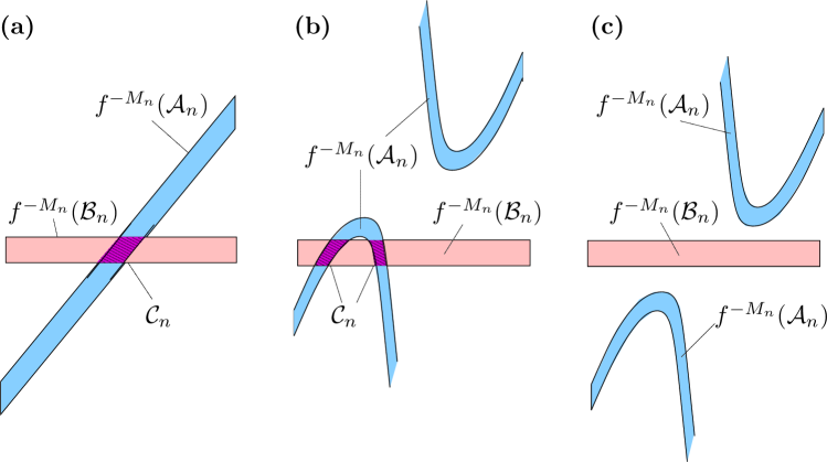
Figure 2.1: The geometry of the critical sets $\mathcal{C}_{n+1}$ in the multiscale analysis: (a) in the standard setting and (b) and (c) in the case of fast returns. Note that the two ‘hooks’ of $f^{M_{n}}(\mathcal{A}^{1}_{n})$ are connected to each other as the set wraps once around the torus, but this is not depicted.

In order to achieve this goal, we first perturb the parameter $\tau_{0}$ in such a way that the slow recurrence conditions $(\mathcal{X})_{n-1}$ and $(\mathcal{Y})_{n}$ still hold, but there is a fast return of $\mathcal{I}_{n}$ to itself. More precisely, the control on the parameter-dependence of the critical sets obtained in [21] is used to shift $\tau_{0}$ in such a way that $I^{1}_{n}+k\omega\cap I^{2}_{n}\neq\emptyset$ for some relatively small $k\geq 0$. For the second component of $\mathcal{C}_{n}$, on which we concentrate now, this implies that when $\mathcal{A}_{n}^{2}=(I^{2}_{n}-(M_{n}-1)\omega)\times C$ is iterated forwards, it passes through the critical region $I^{1}_{n}\times\mathbb{T}^{1}$ before it approaches $I^{2}_{n}\times\mathbb{T}^{1}$ to intersect with the $M_{n}$-th preimage of $\mathcal{B}^{2}_{n}=(I^{2}_{n}+(M_{n}+1)\omega)$.

This results in a drastic change in the geometry of the resulting image $f^{M_{n}}(\mathcal{A}^{2}_{n})$, and qualitatively the situation then looks as in Figure 2.1(b). The set $f^{M_{n}}(\mathcal{A}^{2}_{n})$ now has two ‘hooks’, and the vertical extension of the gap between these hooks is greater than that of $f^{-M_{n}}(\mathcal{B}^{2}_{n})$. A more detailed explanation for this behaviour is difficult to give at this stage, but will be provided in Section 5 (see Figures 5.1 and 5.2). Moreover, when the parameter $\tau$ is varied further, the hooks move both horizontally and, more importantly, also vertically with $\tau$, whereas the set $f^{-M_{n}}(\mathcal{B}^{2}_{n})$ remains more or less stable. As a consequence, for some parameters $\tau$ the involved sets have to reach a position where their intersection remains empty, as shown in Figure 2.1(c). A similar picture holds simultaneously for the first component $f^{M_{n}}(\mathcal{A}_{n}^{1})\cap f^{-M_{n}}(\mathcal{B}_{n}^{1})$, thus showing that $\mathcal{C}_{n}=\emptyset$ for some $\tau$ close to $\tau_{0}$. As mentioned above, this will allow to complete the proof of Theorem 1.1 via Proposition 4.7.

For the rigorous implementation of this proof, the major task will be to describe the geometry and parameter-dependence of the set $f^{M_{n}}(\mathcal{A}_{n})$. Instead of trying to define precisely what it means to be ‘hook-shaped’, we show that $f^{M_{n}}(\mathcal{A}_{n}^{\iota})\cap(\mathbb{T}^{1}\times E)$ is contained in the disjoint union of certain polygons $\mathcal{L}$ and $\mathcal{R}$. We provide quantitative estimates on the shape and position of these sets which imply that the preimage $f^{-M_{n}}(\mathcal{B}_{n}^{\iota})$, which is a thin and more or less horizontal strip contained in $\mathbb{T}^{1}\times E$, cannot intersect both of them at the same time. Moreover, we show that by moving $\tau$ it is possible to force an intersection with $\mathcal{L}$ at one parameter near $\tau_{0}$ and with $\mathcal{R}$ at another one, which implies that for some intermediate parameter there is no intersection with either of them.

The precise quantitative version of our main result, including the explicit characterisation of the set $\mathcal{U}$ in terms of $\mathcal{C}^{1}$-estimates, is given in the next section. Section 4 collects some further information and statements on the multiscale analysis scheme from [16, 21, 17]. In Section 5, we state the properties and quantitative estimates for the polygons $\mathcal{L}$ and $\mathcal{R}$ containing $f^{M_{n}}(\mathcal{A}_{n}^{\iota})$ and on $f^{-M_{n}}(\mathcal{B}_{n}^{\iota})$ and show how these statements imply the main result. The proofs of these estimates are then given in Section 6.

3 Quantitative version of the main result

We first state the precise conditions on the geometry of the considered parameters families, which were only circumscribed in the previous section.

I. Diophantine condition. We say $\omega\in\mathbb{T}^{1}$ satisfies the Diophantine condition with constants $\gamma$ and $\nu$ if

(3.1) $$d(n\omega,0)\ >\ \gamma\cdot|n|^{-\nu}\quad\forall n\in\mathbb{Z}\setminus\{0\}\ .$$

By $\mathcal{D}(\gamma,\nu)$, we denote the set of $\omega\in\mathbb{T}^{1}$ which satisfy (3.1).

II. Critical regions. Let $E=[e^{-},e^{+}]$ and $C=[c^{-},c^{+}]$ be two non-empty, compact and disjoint subintervals of $\mathbb{T}^{1}$. We assume that for all $\tau\in\mathbb{T}^{1}$ there exists a set ${\cal I}_{0}(\tau)\subseteq\mathbb{T}^{1}$ which is the union of two disjoint open intervals $I_{0}^{1}(\tau),I_{0}^{2}(\tau)$ and satisfies

($${\cal A}1 f_{\tau,\theta}(\mbox{cl}(\mathbb{T}^{1}\setminus E))\ \subseteq\ \mbox{int}(C)\ \ \ \ \ \forall\theta\notin{\cal I}_{0}(\tau)\ .$$)

Note that this implies

($${\cal A}1^{\prime} f_{\tau,\theta}^{-1}(\mbox{cl}(\mathbb{T}^{1}\setminus C))\ \subseteq\ \mbox{int}(E)\ \ \ \ \ \forall\theta\notin{\cal I}_{0}(\tau)+\omega\ .$$)

III. Bounds on the derivatives. Concerning the derivatives of the fibre maps $f_{\tau,\theta}$, we assume that for some $\alpha>1$ and $p\geq 2$ we have

($${\cal A}2 \alpha^{-p}\ <\ \partial_{x}f_{\tau,\theta}(x)\ <\ \alpha^{p}\hskip 20.00003pt\quad\forall(\theta,x)\in\mathbb{T}^{2}\ ;$$)

($${\cal A}3 \hskip 30.00005pt\partial_{x}f_{\tau,\theta}(x)\ >\ \alpha^{2/p}\hskip 41.00012pt\quad\forall(\theta,x)\in\mathbb{T}^{1}\times E\ ;$$)

($${\cal A}4 \hskip 30.00005pt\partial_{x}f_{\tau,\theta}(x)\ <\ \alpha^{-2/p}\hskip 41.00012pt\quad\forall(\theta,x)\in\mathbb{T}^{1}\times C\ .$$)

Further, we fix $S>0$ such that

($${\cal A}5 |\partial_{\theta}f_{\tau,\theta}(x)|\ <\ S\ \ \ \ \ \forall(\theta,x)\in\mathbb{T}^{2}\ .$$)

IV. Transversal Intersections. The following condition ensures that the image of $I_{0}^{\iota}(\tau)\times C$ crosses $(I^{\iota}_{0}(\tau)+\omega)\times E$ exactly once and not several times.

($${\cal A}6 \begin{array}[]{l}\exists!\theta_{\iota}^{1}\in I_{0}^{\iota}(\tau)\textrm{ with }f_{\tau,\theta_{\iota}^{1}}(c^{+})=e^{-}\textrm{ \ and }\\ \exists!\theta_{\iota}^{2}\in I_{0}^{\iota}(\tau)\textrm{ with }f_{\tau,\theta_{\iota}^{2}}(c^{-})=e^{+}\ .\end{array}$$)

The slope of $f(I^{\iota}_{0}(\tau)\times C)$ is controlled by

($${\cal A}7 \left\{\begin{array}[]{ll}&\partial_{\theta}f_{\tau,\theta}(x)\ <\ -s\ \ \ \ \ \forall(\theta,x)\in I_{0}^{1}(\tau)\times\mathbb{T}^{1}\\ &\partial_{\theta}f_{\tau,\theta}(x)\ >\quad\,s\ \ \ \ \ \forall(\theta,x)\in I_{0}^{2}(\tau)\times\mathbb{T}^{1}\end{array}\right.\ \ ,$$)

where $s$ is a constant with $0<s<S$. Note that thus $f(I^{\iota}_{0}(\tau)\times C)$ crosses $(I^{\iota}_{0}(\tau)+\omega)\times E$ ‘downwards’ if $\iota=1$ and ‘upwards’, as in Figure 2.1(a), if $\iota=2$.

V. Dependence on $\tau$. First, we assume that $f_{\tau,\theta}(x)$ is monotonically increasing with respect to $\tau$, and we fix upper and lower bounds $L,\ell>0$ on $\partial_{\tau}f_{\tau,\theta}(x)$, that is,

($${\cal A}8 \ell<\partial_{\tau}f_{\tau,\theta}(x)\ <\ L\ \ \ \ \ \forall(\theta,x)\in\mathbb{T}^{2}\ .$$)

Writing $I^{\iota}_{0}(\tau)=(a^{\iota}_{0}(\tau),b^{\iota}_{0}(\tau))$ for $\iota=1,2$, we further assume that the functions $a^{\iota}_{0},b^{\iota}_{0}$ are continuously differentiable with respect to $\tau$. Then we assume

($${\cal A}9 \inf_{\tau\in\mathbb{T}^{1}}\left(\min\{\partial_{\tau}a^{1}_{0}(\tau),\partial_{\tau}b^{1}_{0}(\tau)\}-\max\{\partial_{\tau}a^{2}_{0}(\tau),\partial_{\tau}b^{2}_{0}(\tau)\}\right)\ >\ \ell/S\ .\\$$)

This ensures that the two components of $\mathcal{I}_{0}$ ‘move relative to each other’ with minimal speed $\ell/S$. Finally, by increasing $L$ further if necessary, we can assume that

($$\mathcal{A}10 \sup_{\tau\in\mathbb{T}^{1}}\max\{|\partial_{\tau}a^{1}_{0}(\tau)|,|\partial_{\tau}b^{1}_{0}(\tau)|,|\partial_{\tau}a^{2}_{0}(\tau)|,|\partial_{\tau}b^{2}_{0}(\tau)|\}\ <\ 2L/s\ .$$)

Given $A\subseteq\mathbb{T}^{1}$, we denote by $|A|$ the Lebesgue measure of $A$. In particular, if $A$ is an interval, then $|A|$ is simply its length. The quantitative version of Theorem 1.1, with an explicit characterisation of the set $\mathcal{U}$, now reads as follows.

Theorem 3.1.

Let $\omega\in\mathcal{D}(\gamma,\nu)$, $\delta>0$ and suppose $\hat{f}\in\mathcal{P}_{\omega}$ satisfies the conditions (${\cal A}1$)– ($\mathcal{A}10$) above. Let $\varepsilon_{0}=\sup_{\tau\in\mathbb{T}^{1}}\max\left\{|I^{1}_{0}(\tau)|,|I^{2}_{0}(\tau)|\right\}$.

Then there exist contants $\alpha_{*}=\alpha_{*}(\delta,\gamma,\nu,p,S,s,\ell,L)>0$ and $\varepsilon_{*}=\varepsilon_{*}(\delta,\gamma,\nu,p,S,s,\ell,L)$ such that if $\alpha>\alpha_{*}$ and $\varepsilon_{0}<\varepsilon_{*}$, then there exists a set $\Lambda^{\hat{f}}\subseteq\mathbb{T}^{1}$ of measure at least $1-\delta$ with the property that

• for all $\tau\in\Lambda^{\hat{f}}$, the map $f_{\tau}$ has a (unique) SNA and the dynamics of $f_{\tau}$ are minimal;

• $\Lambda^{\hat{f}}\subseteq\partial\mathcal{M}(\hat{f})$.

Note that since the above conditions (${\cal A}1$)–($\mathcal{A}10$) are all $\mathcal{C}^{1}$-open, this directly implies Theorem 1.1.

4 Preliminaries on the multiscale analysis

As mentioned before, the existence of SNA and the minimality of the dynamics in Theorems 1.1 and 3.1 are already contained in [16, 21]. However, in order to build on these results, we need restate them in a precise way and provide some additional quantitative information. In particular, this concerns the slow recurrence conditions $(\mathcal{X})_{n}$ and $(\mathcal{Y})_{n}$, which are replaced by the following stronger versions.

$$(\mathcal{X^{\prime}})_{n} d(\mathcal{I}_{j},\mathcal{X}_{j})\ >\ 9\varepsilon_{j}\qquad\forall j=0,\ldots,n,$$

$$(\mathcal{Y}^{\prime})_{n} d((\mathcal{I}_{j}-(M_{j}-1)\omega)\cup(\mathcal{I}_{j}+(M_{j}+1)\omega),\mathcal{Y}_{j-1})\ >\ 2\varepsilon_{j-1}\quad\forall j=1,\ldots,n\ .$$

With these notions, we can restate [21, Theorem 3.1] as follows. The information on the sequences $(K_{j})_{j\in\mathbb{N}},(M_{j})_{j\in\mathbb{N}}$ and $(\varepsilon_{j})_{j\in\mathbb{N}}$ is taken from the proof of this theorem.

Theorem 4.1 ([21]).

Let $\omega\in\mathcal{D}(\gamma,\nu)$, $\delta>0$ and suppose $\hat{f}\in\mathcal{P}_{\omega}$ satisfies the conditions (${\cal A}1$)–($\mathcal{A}10$) above. Let $\varepsilon_{0}=\sup_{\tau\in\mathbb{T}^{1}}\max\{|I^{1}_{0}(\tau)|,|I^{2}_{0}(\tau)|\}$. Then there exist constants $\alpha_{*}^{\prime}$ and $\varepsilon_{*}^{\prime}$, both depending on the constants $\delta,\gamma,\nu,p,S,s,\ell,L$ above, with the property that if $\alpha>\alpha_{*}^{\prime}$ and $\varepsilon_{0}<\varepsilon_{*}^{\prime}$, then there exists a set $\Lambda^{\hat{f}}\subseteq\mathbb{T}^{1}$ of measure at least $1-\delta$ such that for all $\tau\in\Lambda^{\hat{f}}$ the map $f_{\tau}$ has an SNA and minimal dynamics.

Further, for each $\tau\in\Lambda^{\hat{f}}$ there exist sequences $(K_{j})_{j\in\mathbb{N}},(M_{j})_{j\in\mathbb{N}}$ and $(\varepsilon_{j})_{j\in\mathbb{N}}$ such that for all $n\in\mathbb{N}$ the critical regions $\mathcal{I}_{n}$ defined in (2.1)– (2.4) satisfy the slow-recurrence assumptions $(\mathcal{X^{\prime}})_{n}$ and $(\mathcal{Y}^{\prime})_{n}$ and in addition

(4.1) $$\max\{|I^{1}_{n}|,|I^{2}_{n}|\}\ \leq\ \varepsilon_{n}\ .$$

Moreover, the above sequences can be chosen such that $M_{0}=3$, $K_{j}=2^{j+t+2}$ for some $t\geq 4$ which satisfies

(4.2) $$2^{-t}\ \leq\ \log\left(\frac{p^{2}+2}{p^{2}+1}\right)\ ,$$

and for all $j\in\mathbb{N}_{0}$ we have

(4.3) $$M_{j+1} \in \left[\alpha^{M_{j}/2pq},2\alpha^{M_{j}/pq}\right]\ ,$$

(4.4) $$\varepsilon_{j+1} \in [2\alpha^{-M_{j}/p}/s,2\alpha^{-M_{j}/2p}/s]\ ,$$

where $q=\max\{8,4\nu\}$.

Remark 4.2.

We note that there are actually two small modifications in Theorem 4.1 in comparison to [21, Theorem 3.1].

The first is just the correction of an unfortunate typo. In the statement of $(\mathcal{Y}^{\prime})_{n}$ on [21, Page 1488], the given lower bound is $2\varepsilon_{j}$ instead of $2\varepsilon_{j-1}$. However, it can be seen from estimate (4.21) in [21, Lemma 4.7] and its use in the proof of [21, Lemma 4.9] that all the respective statements hold with a lower bound of $2\varepsilon_{j-1}$.

The second modification concerns the definition of $\mathcal{Y}_{n}$ in $(\mathcal{Y})_{n}$, where the index $l$ in the union on the right runs from $-M_{j}$ to $M_{j}+2$, instead of only from $-M_{j}+1$ to $M_{j}+1$ as in the respective definition in [21]. This is an adaption that we need to make for technical reasons. However, this difference does not have any influence on the proofs in [21], which go through in literally the same way, so that the result remains valid in the above form.

The statement of Theorem 4.1 provides the basis for our further analysis. In addition we will need a number of technical lemmas which allow to control the behaviour of orbits of finite length on time-scales corresponding to the slow-recurrence conditions $(\mathcal{X})_{n}$ and $(\mathcal{Y})_{n}$. The philosophy of these statements is the following. Suppose $(\theta_{0},x_{0})\in\mathbb{T}^{1}\times C$ and let $(\theta_{n},x_{n})=f^{n}_{\tau}(\theta_{0},x_{0})$. Then the almost invariance of the contracting region, given by (${\cal A}1$), implies that $x_{n}\in C$ as long as $\theta_{j}\notin\mathcal{I}_{0}$ for all $j=0,\ldots,n-1$. Thus, an orbit that starts in the contracting region will stay there as long as its $\theta$-coordinate stays away from the critical region $\mathcal{I}_{0}$. The key observation on which the whole multiscale analysis hinges is the fact that even for longer orbits, whose first coordinates do visit the critical regions, a similar statement nevertheless holds at least ‘most of the times’. In order to make this precise, let

(4.5) $$\mathcal{V}^{-}_{n}\ =\ \bigcup_{j=0}^{n}\bigcup_{l=-M_{j}+2}^{0}(\mathcal{I}_{j}+l\omega)\quad\textrm{and}\quad\mathcal{W}^{+}_{n}:=\bigcup_{j=0}^{n}\bigcup_{l=1}^{M_{j}+1}(\mathcal{I}_{j}+l\omega)$$

Then we have

Lemma 4.3 ([17, Lemma 4.4], Forwards Iteration).

Suppose $f_{\tau}$ satisfies (${\cal A}1$) and $(\mathcal{Y})_{n-1}$ holds. Let $\mathcal{L}\geq 0$ be the first integer such that $\theta_{\mathcal{L}}\in\mathcal{I}_{n}$. Then

$$(\mathcal{B}1)_{n} \left\{\begin{array}[]{lll}&\theta_{0}\notin\mathcal{V}^{-}_{n-1}\\ &x_{0}\notin\mathrm{int}(E)\end{array}\right.$$

implies that

$$(\mathcal{C}1)_{n} \theta_{m}\notin\mathcal{W}^{+}_{n-1}\ \Rightarrow\ x_{m}\in\mathrm{int}(C)\quad\forall m=1,\ldots,\mathcal{L}\ .$$

We note that in [17] the lemma is stated under the additional assumption that $(\mathcal{X})_{n-1}$ holds as well, but this is actually not needed and is not used in the proof. The same applies to Lemma 4.4 below.

It can be seen from (4.1)–(4.4) that for large $\alpha$ the exceptional sets $\mathcal{V}^{-}_{n}$ and $\mathcal{W}^{+}_{n}$ are very small. Hence, an orbit starting in $(\mathbb{T}^{1}\setminus\mathcal{V}^{-}_{n})\times C$ typically remains trapped in the contracting region most of the time, until it enters $\mathcal{I}_{n+1}\times C$. A similar statement holds for the backwards iteration. Let

(4.6) $$\mathcal{V}_{n}^{+}\ =\ \bigcup_{j=0}^{n}\bigcup_{l=1}^{M_{j}}(\mathcal{I}_{j}+l\omega)\quad\textrm{and}\quad\mathcal{W}^{-}_{n}\ =\ \bigcup_{j=0}^{n}\bigcup_{l=-M_{j}+1}^{0}(\mathcal{I}_{j}+l\omega)\ .$$

Lemma 4.4 ([17, Lemma 4.4], Backwards Iteration).

Suppose $f_{\tau}$ satisfies (${\cal A}1$) and $(\mathcal{Y})_{n-1}$ holds. Let $\mathcal{R}\geq 0$ be the first integer such that $\theta_{-\mathcal{R}}\in\mathcal{I}_{n}+\omega$. Then

$$(\mathcal{B}2)_{n} \left\{\begin{array}[]{lll}&\theta_{0}\notin\mathcal{V}_{n-1}^{+}\\ &x_{0}\notin\mathrm{int}(C)\end{array},\right.$$

implies

$$(\mathcal{C}2)_{n} \theta_{-m}\notin\mathcal{W}^{-}_{n-1}\ \Rightarrow\ x_{-m}\in\mathrm{int}(E)\quad\forall m=1,\ldots,\mathcal{R}\ .$$

It should be emphasized here that the above two statements are purely combinatorial in nature, and only rely on the almost invariance of the contracting and expanding region given by (${\cal A}1$). If they are combined with quantitative estimates on the derivates like in (${\cal A}2$)–(${\cal A}7$), they can be used to obtain a wealth of further information on finite-time Lyapunov exponents or the geometry of iterates of suitable small curves or sets. The basis of such a quantified analysis are suitable estimates on the proportion of time spent in the contracting or expanding region. To that end, given $\tau,\theta_{0},x_{0}$ and $0\leq m\leq N$, let

(4.7) $$\mathcal{P}_{m}^{N} = \#\{l\in[m,N-1]:x_{l}\in C\}\ ,$$

(4.8) $$\mathcal{Q}_{m}^{N} = \#\{l\in[m,N-1]:x_{-l}\in E\}\ .$$

Further, let $\beta_{0}=1$ and $\beta_{n}=\prod_{j=0}^{n-1}(1-K_{j}^{-1})$. Note that due to the choice of the $K_{j}$ in Theorem 4.1 and (4.2), we have

(4.9) $$\frac{2}{p}\beta_{n}-(1-\beta_{n})p\ \geq\ \frac{1}{p}$$

for all $n\in\mathbb{N}$. Lemmas 4.3 and 4.4 now lead to the following quantitative estimates.

Lemma 4.5 ([17, Lemma 4.6]).

Suppose $f_{\tau}$ satisfies (${\cal A}1$) and conditions $(\mathcal{X})_{n-1}$ and $(\mathcal{Y})_{n-1}$ hold. Let $0<L_{1}<L_{2}<\ldots<L_{J}=\mathcal{L}$ denote all those times $L_{i}\leq\mathcal{L}$ for which $\theta_{L_{i}}\in\mathcal{I}_{n-1}$. Further, assume that $(\mathcal{B}1)_{n}$ holds. Then for each $j=1,\ldots,J$, we have

(4.10) $$\mathcal{P}_{m}^{L_{j}}\geq\beta_{n}(L_{j}-m)\ \ \forall m=0,\ldots,L_{j}-1.$$

Further $x_{L_{j}}\in C,\ \forall j=1,\ldots,J$.

Similarly, let $0<R_{1}<\ldots<R_{J}=\mathcal{R}$ denote are all those times $R_{i}\leq\mathcal{R}$ for which $\theta_{-R_{i}}\in\mathcal{I}_{n-1}+\omega$. Then for each $j=1,\ldots,J$, we have

(4.11) $$\mathcal{Q}_{m}^{R_{j}}\geq\beta_{n}(R_{j}-m)\ \ \forall m=0,\ldots,R_{j}-1.$$

Further $x_{-R_{j}}\in E,\ \forall j=1,\ldots,J$.

These estimates can be used to obtain precise control on the size and parameter dependence of the critical intervals.

Proposition 4.6 ([16, Proposition 3.11] and [21, Lemma 4.5]).

Suppose $\hat{f}\in\mathcal{P}_{\omega}$ satisfies (${\cal A}1$)-($\mathcal{A}10$), $(\mathcal{X})_{n-1},\ (\mathcal{Y})_{n-1}$ hold for some $n\geq 1$ and $\alpha$ is sufficiently large. Then the two connected components of $\mathcal{I}_{n}(\tau)$, denoted as $I_{n}^{\iota}(\tau)=(a_{n}^{\iota}(\tau),\ b_{n}^{\iota}(\tau)),\ \iota=1,2$, are differentiable in $\tau$. Further, we have

(4.12) $$|I_{n}^{\iota}(\tau)|\leq\varepsilon_{n},\ \ \iota=1,2,$$

(4.13) $$\min\{\partial_{\tau}a^{1}_{n}(\tau),\partial_{\tau}b^{1}_{n}(\tau)\}-\max\{\partial_{\tau}a^{2}_{n}(\tau),\partial_{\tau}b^{2}_{n}(\tau)\}\ >\ \ell/S\ ,$$

(4.14) $$|\partial_{\tau}I_{n}^{\iota}(\tau)|\ \leq\ 2L/s,\ \ \iota=1,2,$$

where $|\partial_{\tau}I_{n}^{\iota}(\tau)|=\max\{|\partial_{\tau}a_{n}^{\iota}(\tau)|,\ |\partial_{\tau}b_{n}^{\iota}(\tau)|\},\ \iota=1,2$.

Note that for $n=0$, the respective estimates hold by assumption.

As a first consequence of the above statements, we obtain that the emptyness of a critical region implies mode-locking.

Proposition 4.7.

The constants $\alpha_{*}^{\prime}$ and $\varepsilon_{*}^{\prime}$ in Theorem 4.1 can be chosen such that if $\alpha>\alpha_{*}$ and $\varepsilon_{0}<\varepsilon_{*}$, then the following holds.

Let $K_{0},\ldots,K_{n}$ be chosen as in Theorem 4.1. Further, suppose that for some $\tau\in\mathbb{T}^{1}$ the numbers $M_{0},\ldots,M_{n}$ can be chosen such that (4.3) holds for $j=0,\ldots,n-1$ and conditions $(\mathcal{X})_{n-1}$ and $(\mathcal{Y})_{n}$ are satisfied, but $\mathcal{C}_{n}=\emptyset$. Then $f_{\tau}$ has an attracting continuous invariant graph. In particular, $f_{\tau}$ is mode-locked.

Proof.

For convenience, we omit the parameter $\tau$ throughout the proof. First, by Proposition 4.6, we have $|I_{j}^{\iota}|\leq\varepsilon_{j},\ \iota=1,2,\ j=0,\ldots,n$. Then by (4.3), (4.4) and (4.5), we know that $\mathcal{W}_{n}^{+},\ \mathcal{V}_{n}^{-}$ are unions of small intervals which satisfy the following estimates

(4.15) $$\mathrm{Leb}(\mathcal{W}^{+}_{n})\leq\sum_{j=0}^{n}(M_{j}+1)\varepsilon_{j}<2M_{0}\varepsilon_{0}+\frac{8}{s}\cdot\sum_{j=1}^{n}\alpha^{-\frac{M_{j-1}}{4p}}<\frac{1}{2(p^{2}+2)},$$

(4.16) $$\mathrm{Leb}(\mathcal{V}_{n}^{-})\leq\sum_{j=0}^{n}M_{j}\varepsilon_{j}\leq M_{0}\varepsilon_{0}+\frac{4}{s}\cdot\sum_{j=1}^{n}\alpha^{-\frac{M_{j-1}}{4p}}<\frac{1}{4(p^{2}+2)},$$

for $\alpha$ large and $\varepsilon_{0}$ small. Thus, there must be some interval $\mathcal{J}^{\prime}\subseteq\mathbb{T}^{1}\setminus(\mathcal{V}_{n}^{-}\cup\mathcal{W}^{+}_{n})$. We let $\mathcal{J}^{\prime}=(a^{\prime},b^{\prime})$ and $\lambda=|\mathcal{J}^{\prime}|>0$. Let $\mathcal{J}=[a^{\prime}+\lambda/3,\ b^{\prime}-\lambda/3]$. Since $\omega$ is irrational, there must be some $K\in\mathbb{N}$ such that $\mathrm{int}(\mathcal{J}+K\omega)\cap\mathrm{int}(\mathcal{J})\neq\emptyset$ and $b^{\prime}-\lambda/3\in\mathrm{int}(\mathcal{J}+K\omega)$. In particular, we have $\mathcal{J}+K\omega\subseteq\mathcal{J}^{\prime}$. Since $(\mathcal{Y})_{n}$ holds, $\mathcal{I}_{n+1}=\emptyset$ and $\mathcal{J}\cap(\mathcal{W}^{+}\cup\mathcal{V}^{-})=\emptyset$, Lemma 4.3 implies

(4.17) $$f^{K}(\mathcal{J}\times C)\ \subseteq\ (\mathcal{J}+K\omega)\times C\ .$$

Hence, we obtain $f^{K}(\mathcal{J}\times C)\cap(\mathcal{J}\times C)\neq\emptyset$, and thus

(4.18) $$f^{(j+1)K}(\mathcal{J}\times C)\cap f^{jK}(\mathcal{J}\times C)\neq\emptyset,\ \ j=1,2,\ldots$$

Moreover, there exists $N>1$, such that $\mathrm{int}(\mathcal{J}+NK\omega)\cap\mathrm{int}(\cal{J})\neq\emptyset$, $a^{\prime}+\lambda/3\in\mathrm{int}(\mathcal{J})+NK\omega$ and $a^{\prime}+\lambda/3\notin\mathcal{J}+(N+1)K\omega$. Then we have $\cup_{j=0}^{N}(\mathcal{J}+jK\omega)=\mathbb{T}^{1}$. By the same reasoning as above, we further have that $f^{NK}(\mathcal{J}\times C)\subseteq(\mathcal{J}+NK\omega)\times C$, and

(4.19) $$f^{NK}(\mathcal{J}\times C)\cap(\mathcal{J}\times C)\neq\emptyset.$$

Consequently, the set

(4.20) $$\mathcal{A}:=\bigcup_{j=0}^{N}f^{jK}(\mathcal{J}\times C)$$

is connected and wraps around the torus in the horizontal direction. In fact, if we assume $N$ to be minimal with the above property, $\mathcal{A}$ horizontally wraps around the torus exactly once. We now claim that $f^{(N+1)K}(\mathcal{J}\times C)\subseteq(\mathcal{J}\times C)\cup f^{K}(\mathcal{J}\times C)$, which immediately implies

(4.21) $$f^{K}(\mathcal{A})\ \subseteq\ \mathcal{A}\ .$$

The reason is the following. Suppose $(\theta,x)\in f^{(N+1)K}(\mathcal{J}\times C)$. Then since $d(K\omega,0)<|\mathcal{J}|$ and due to the choice of $N$ above, there are two possibilities. On the one hand, we may have $\theta\in\mathcal{J}$. In this case, the fact that $\mathcal{J}\cap(\mathcal{W}^{+}_{n}\cup\mathcal{V}_{n}^{-})=\emptyset$ implies, via Lemma 4.3, that $(\theta,x)\in\mathcal{J}\times C$. On the other hand, we may have $\theta-K\omega\in\mathcal{J}$. Then the same argument yields $f^{-K}(\theta,x)\in\mathcal{J}\times C$, and thus $(\theta,x)\in f^{K}(\mathcal{J}\times C)$. In both cases, we have $(\theta,x)\in(\mathcal{J}\times C)\cup f^{K}(\mathcal{J}\times C)$.

Since $\mathcal{W}^{+}_{n}$ is a finite union of small intervals and $\omega$ is irrational, then by Weyl’s criterion, $\{\theta_{0}+m\omega\}_{m\in\mathbb{N}}$ is equidistributed in $\mathbb{T}^{1}$ for all $\theta_{0}\in\mathbb{T}^{1}$, which means that

(4.22) $$\lim_{m\rightarrow\infty}\frac{1}{m}\sum_{j=0}^{m-1}\textbf{1}_{\mathcal{W}_{n}^{+}}(\theta_{0}+m\omega)=\mathrm{Leb}(\mathcal{W}^{+}_{n}).$$

Let $(\theta_{0},x_{0})\in\mathcal{J}\times C$. Using Lemma 4.3 in combination with (4.22), (${\cal A}2$) and (${\cal A}4$), we obtain

$$\varlimsup\frac{1}{n}\log\partial_{x}f^{n}_{\theta_{0}}(x_{0})\ \leq\ (-2/p+(2/p+p)\mathrm{Leb}(\mathcal{W}^{+}_{n}))\log\alpha\ \stackrel{{\scriptstyle\eqref{esti_v_n}}}{{\leq}}\ -\log\alpha/p\ .$$

By the definition of $\mathcal{A}$, it is now easy to show that all points in $\mathcal{A}$ have negative vertical Lyapunov exponents. By [29, Corollary 1.15], this implies that the compact invariant set $\bigcap_{n\in\mathbb{N}}f^{nK}(\mathcal{A})$ is the graph of a continuous curve with negative vertical Lyapunov exponent. Since this implies mode-locking [18], the proof is complete. ∎

One task which will frequently come up in the proof of the main theorem is to control the geometry of small arcs whose iterates remain in the contracting region (resp. expanding region) most of the time. The following statements cover all these situations.

Lemma 4.8 (Forwards Iteration).

Suppose $f_{\tau}$ satisfies assumptions (${\cal A}1$), (${\cal A}2$), (${\cal A}4$), (${\cal A}5$), (${\cal A}7$) and the slow recurrence conditions $(\mathcal{X})_{n-1}$ and $(\mathcal{Y})_{n-1}$ hold. Let $I\subset\mathbb{T}^{1}$ be an interval and $N\geq 1$. Then, if $\alpha$ is sufficiently large and $\varepsilon_{0}$ is sufficiently small, the following are true.

If $\phi^{1}:I\rightarrow\mathbb{T}^{1}\setminus\mathrm{int}(E)$ is a $\mathcal{C}^{1}$-curve and

$$(\mathcal{D}1)_{n} \left\{\begin{array}[]{llll}&I\cap\mathcal{V}_{n-1}^{-}=\emptyset,\\ &I+N\omega\subset\mathcal{I}_{n-1},\\ &(I+l\omega)\cap\mathcal{I}_{n}=\emptyset,\ \forall\ l=0,1,\ldots,N-1,\\ \end{array}\right.$$

then we have

(4.23) $$\left|\partial_{\theta}f^{N}_{\tau,\theta}\left(\phi^{1}(\theta)\right)\right|\ \leq\ \sum_{l=0}^{N-1}\alpha^{-l/p}S+\alpha^{-N/p}\left|\partial_{\theta}\phi^{1}(\theta)\right|\ .\$$

Further, we also have

• if $I+N\omega\subset I_{n-1}^{1}$, then

  (4.24) $$\begin{split}-S-\frac{S}{\alpha^{1/p}-1}-\alpha^{-\frac{N+1}{p}}&\left|\partial_{\theta}\phi^{1}(\theta)\right|\ \ \leq\ \partial_{\theta}f_{\tau,\theta}^{N+1}(\phi^{1}(\theta))\ \\ &\ \leq\ -s+\frac{S}{\alpha^{1/p}-1}+\alpha^{-\frac{N+1}{p}}\left|\partial_{\theta}\phi^{1}(\theta)\right|\ ;\end{split}$$

• if $I+N\omega\subset I_{n-1}^{2}$, then

  (4.25) $$\begin{split}s-\frac{S}{\alpha^{1/p}-1}-\alpha^{-\frac{N+1}{p}}&\left|\partial_{\theta}\phi^{1}(\theta)\right|\ \leq\ \partial_{\theta}f_{\tau,\theta}^{N+1}(\phi(\theta))\ \\ &\ \leq\ S+\frac{S}{\alpha^{1/p}-1}+\alpha^{-\frac{N+1}{p}}\left|\partial_{\theta}\phi^{1}(\theta)\right|\ .\end{split}$$

Moreover, if $\phi^{1},\phi^{2}:I\rightarrow\mathbb{T}^{1}\setminus\mathrm{int}(E)$ are $\mathcal{C}^{1}$-curves and $(\mathcal{D}1)_{n}$ holds, then

(4.26) $$\left|f_{\tau,\theta}^{j}(\phi^{1}(\theta))-f_{\tau,\theta}^{j}(\phi^{2}(\theta))\right|\ \leq\ \alpha^{-j/p}\left|\phi^{1}(\theta)-\phi^{2}(\theta)\right|\ \quad\textrm{for}\ \ j=N,N+1.$$

Proof.

Again, we omit the parameter $\tau$ during the proof. Moreover, we assume that the parameter $\alpha$ is sufficiently large, and all estimates below should be understood under this premise. For any $m\geq 1$, $\theta\in I$ and $\iota=1,2$, we let $\phi_{m}^{\iota}(\theta)=f_{\theta}^{m}(\phi^{\iota}(\theta))$. Set $\theta_{0}:=\theta\in I$ and $x_{0}:=\phi^{\iota}(\theta_{0})\notin\mathrm{int}(E)$. Then we have

(4.27) $$\begin{split}\partial_{\theta}\phi_{m}^{\iota}(\theta)&\ =\ \left(\partial_{\theta}f_{\theta_{m-1}}\right)(x_{m-1})+\left(\partial_{x}f_{\theta_{m-1}}\right)(x_{m-1})\cdot\partial_{\theta}f_{\theta_{0}}^{m-1}\left(\phi^{\iota}(\theta_{0})\right)=\cdots\\ &\ =\ \partial_{\theta}f_{\theta_{m-1}}(x_{m-1})+\sum_{l=0}^{m-2}\big{(}\partial_{x}f_{{\theta_{l+1}}}^{m-l-1}\big{)}(x_{l+1})\cdot(\partial_{\theta}f_{\theta_{l}})(x_{l})\\ &\ \ +\big{(}\partial_{x}f_{\theta_{0}}^{m}\big{)}(x_{0})\cdot\partial_{\theta}\phi^{\iota}(\theta),\end{split}$$

where

(4.28) $$\big{(}\partial_{x}f_{\theta_{l+1}}^{m-l-1}\big{)}(x_{l+1})\ =\ \prod_{j=l+1}^{m-1}\big{(}\partial_{x}f_{\theta_{j}}\big{)}(x_{j}),\ \ l=-1,0,\ldots,m-2.$$

Taking $m=N$ we can apply Lemma 4.5, whose conditions hold due to $(\mathcal{D}1)_{n}$. We thus obtain

$$\mathcal{P}_{l+1}^{N}\ \geq\ \beta_{n}(N-l-1),$$

which implies that

$$\begin{split}\left|\left(\partial_{x}f_{\theta_{l+1}}^{N-l-1}\right)(x_{l+1})\right|&\ \leq\ \alpha^{-\frac{2}{p}\mathcal{P}_{l+1}^{N}}\alpha^{p(N-l-1-\mathcal{P}_{l+1}^{N})}\\ &\ \leq\ \left(\alpha^{-\frac{2}{p}\beta_{n}+(1-\beta_{n})p}\right)^{N-l-1}\ \stackrel{{\scriptstyle\eqref{e.beta}}}{{\leq}}\ \alpha^{-\frac{N-l-1}{p}}\ .\end{split}$$

As $|\partial_{\theta}f_{\theta_{l}}|\ \leq\ S,\ \forall l$ by (${\cal A}5$), this yields the estimate (4.23). Further, since

$$\left|\phi_{N}^{1}(\theta)-\phi_{N}^{2}(\theta)\right|\ =\ \left|\partial_{x}f_{\theta_{0}}^{N}(\xi_{0})\right|\cdot\left|\phi^{1}(\theta)-\phi^{2}(\theta)\right|\ \leq\ \alpha^{-N/p}\left|\phi^{1}(\theta)-\phi^{2}(\theta)\right|$$

for some $\xi_{0}\notin\mathrm{int}(E)$ between $\phi^{1}(\theta)$ and $\phi^{2}(\theta)$, we also obtain (4.26) for $j=N$ in the same way. In order to show (4.26) for $j=N+1$, note that $\left[\phi_{N}^{1}(\theta),\phi_{N}^{2}(\theta)\right]\subseteq C$ by Lemma 4.5. There exists $\eta\in\left[\phi^{1}_{N}(\theta),\phi^{2}_{N}(\theta)\right]$ such that

$$|f_{\theta_{0}+N\omega}(\phi_{N}^{1}(\theta))-f_{\theta_{0}+N\omega}(\phi_{N}^{2}(\theta))|\ =\ |\partial_{x}f_{\theta_{0}+N\omega}(\eta)||\phi_{N}^{1}(\theta)-\phi_{N}^{1}(\theta)|$$

$$\stackrel{{\scriptstyle\eqref{eq:bounds3}}}{{\leq}} \alpha^{-2/p}|\phi_{N}^{1}(\theta)-\phi_{N}^{2}(\theta)|\ \leq\ \alpha^{-\frac{N+1}{p}}|\phi^{1}(\theta)-\phi^{2}(\theta)|\ .$$

Finally, in order to show (i), suppose $I+N\omega\subset I_{n-1}^{1}$. Then we have

$$\partial_{\theta}f_{\theta}^{N+1}(\phi^{\iota}(\theta))=(\partial_{\theta}f_{\theta_{N}})(x_{N})+(\partial_{x}f_{\theta_{N}})(x_{N})\partial_{\theta}\phi_{N}^{\iota}(\theta).$$

Since $\theta_{N}\in I_{n-1}^{1}\subset I_{0}^{1}$ and $x_{N}=\phi_{N}^{\iota}(\theta)\in C$, we obtain (4.24) from (4.23), (${\cal A}5$) and (${\cal A}7$), provided that $\alpha$ is large enough. The proof of (ii) is analogous. ∎

A similar statement holds for the backwards iteration.

Lemma 4.9 (Backwards Iteration).

Suppose $f$ satisfies the conditions (${\cal A}1$)-(${\cal A}3$), (${\cal A}5$), (${\cal A}7$) and the slow recurrence conditions $(\mathcal{X})_{n-1}$ and $(\mathcal{Y})_{n-1}$ hold. Let $I\subset\mathbb{T}^{1}$ be an interval and $N\geq 1$. Then, if $\alpha$ is sufficiently large and $\varepsilon_{0}$ is sufficiently small, the following are true.

If $\phi^{1},\phi^{2}:I\to\mathbb{T}^{1}\setminus\mathrm{int}(C)$ are $\mathcal{C}^{1}$-curves and

$$(\mathcal{D}2)_{n} \left\{\begin{array}[]{llll}&I\cap\mathcal{V}_{n-1}^{+}=\emptyset,\\ &I-N\omega\subset\mathcal{I}_{n-1}+\omega,\\ &(I-l\omega)\cap(\mathcal{I}_{n}+\omega)=\emptyset,\ \forall\ l=0,1,\ldots,N-1,\\ \end{array}\right.$$

then we have

(4.29) $$\left|\partial_{\theta}f_{\theta}^{-N}\left(\phi^{\iota}(\theta)\right)\right|\ \leq\ \sum_{l=1}^{N}\alpha^{-l/p}S+\alpha^{-\frac{N+1}{p}}\left|\partial_{\theta}\phi^{\iota}(\theta)\right|\ ,\quad\iota=1,2,$$

and

(4.30) $$\left|f_{\theta}^{-N}\left(\phi^{1}(\theta)\right)-f_{\theta}^{-N}\left(\phi^{2}(\theta)\right)\right|\ \leq\ \alpha^{-N/p}\left|\phi^{1}(\theta)-\phi^{2}(\theta)\right|\ .$$

Proof.

As before, we omit $\tau$. For $\iota=1,2$, let $\phi_{-N}^{\iota}(\theta)=f_{\theta}^{-N}\left(\phi^{\iota}(\theta)\right),\ \theta\in I$. Further, let $\theta_{0}:=\theta\in I$ and $x_{0}:=\phi^{\iota}(\theta_{0})\notin\mathrm{int}(C)$. We proceed in a similar way as in Lemma 4.8, but this time consider the map $f^{-1}$ instead of $f$. Thus, we write $\theta_{l}=\theta_{0}-l\omega$ and $x_{l}=f_{\theta_{0}}^{-l}(x_{0}).$ First, note that

(4.31) $$\partial_{x}f_{\theta}^{-1}(x)\ =\ \frac{1}{(\partial_{x}f_{\theta-\omega})(f_{\theta}^{-1}(x))}\ \in\ (\alpha^{-p},\alpha^{-2/p})\quad\textrm{ if }f^{-1}_{\theta}(x)\in E$$

by (${\cal A}2$), (${\cal A}3$) and

(4.32) $$\partial_{\theta}f_{\theta}^{-1}(x)=-\frac{(\partial_{\theta}f_{\theta-\omega})(f_{\theta}^{-1}(x))}{(\partial_{x}f_{\theta-\omega})(f_{\theta}^{-1}(x))}\ .$$

Similarly to $(\ref{equ-1})$, we have

$$\partial_{\theta}\phi_{-N}^{\iota}(\theta)\ =\ \big{(}\partial_{x}f_{\theta_{0}}^{-N}\big{)}(x_{0})\cdot\partial_{\theta}\phi^{\iota}(\theta_{0})+\sum_{l=0}^{N-1}\big{(}\partial_{x}f_{\theta_{l+1}}^{-(N-l-1)}\big{)}(x_{l+1})\cdot(\partial_{\theta}f_{\theta_{l}}^{-1})(x_{l}).$$

Since condition $(\mathcal{D}2)_{n}$ holds, Lemma 4.5 yields

$$\mathcal{Q}_{l+1}^{N}\geq\beta_{n}(N-l-1),\ \ l=-1,\ldots,N-1.$$

Then

$$\left|\left(\partial_{x}f_{\theta_{l+1}}^{-(N-l-1)}\right)(x_{l+1})\left(\partial_{\theta}f_{\theta_{l}}^{-1}\right)(x_{l})\right|\ =\ \left|\prod_{j=l+1}^{N-1}\left(\partial_{x}f_{\theta_{j}}^{-1}\right)(x_{j})\frac{\left(\partial_{\theta}f_{\theta_{l+1}}\right)(x_{l+1})}{\left(\partial_{x}f_{\theta_{l+1}}\right)(x_{l+1})}\right|$$

$$= \left|\prod_{j=l}^{N-1}\left(\partial_{x}f_{\theta_{j}}^{-1}\right)(x_{j})\cdot\left(\partial_{\theta}f_{\theta_{l+1}}\right)(x_{l+1})\right|\ \leq\ \alpha^{-\frac{2}{p}}\alpha^{-\frac{2}{p}\mathcal{Q}_{l+1}^{N}}\alpha^{p(N-l-1-\mathcal{Q}_{l+1}^{N})}S$$

$$\leq \alpha^{-\frac{2}{p}}\left(\alpha^{-\frac{2}{p}\beta_{n}+(1-\beta_{n})p}\right)^{N-l-1}S\ \leq\ \alpha^{-\frac{N-l}{p}}S$$

for $l=-1,0,\ldots,N-1$. This implies (4.29). The estimate (4.30) is obtained in a similar way as (4.26). ∎

Remark 4.10.

By equality (4.27), for any $\mathcal{C}^{1}$-curves $\phi^{1},\phi^{2}$ defined on an interval $I\subset\mathbb{T}^{1}$, $m\geq 1$, we obtain that

(4.33) $$|\partial_{\theta}f_{\theta}^{m}(\phi^{\iota}(\theta))|\ \leq\ \sum_{l=0}^{m-1}\alpha^{pl}S+\alpha^{pm}|\partial_{\theta}\phi^{\iota}(\theta)|\ ,\quad\iota=1,2,$$

and

(4.34) $$\alpha^{-pm}\left|\phi^{1}(\theta)-\phi^{2}(\theta)\right|\ \leq\ \left|f_{\theta}^{m}\left(\phi^{1}(\theta)\right)-f_{\theta}^{m}\left(\phi^{2}(\theta)\right)\right|\ \leq\ \alpha^{pm}\left|\phi^{1}(\theta)-\phi^{2}(\theta)\right|\ ,$$

provided $f$ satisfies conditions (${\cal A}2$) and (${\cal A}5$).

5 Geometric estimates and the proof of Theorem 3.1

In this section, we collect the key technical lemmas about the geometry of the intersections shown in Figure 2.1 and show how this information can be combined to prove Theorem 3.1. The proofs of the lemmas will then be given in Section 6.

Recall that our main aim is to render the critical set $\mathcal{C}_{n}$ empty by shifting the parameter $\tau\in\Lambda^{\hat{f}}$. As mentioned in Section 2.2, the first step is to create a fast return of $\mathcal{I}_{n}$ to itself. Thereby, it will be important to ensure that the following condition, which is an itermediate between $(\mathcal{Y})_{n}$ and $(\mathcal{Y}^{\prime})_{n}$, still holds.

$$(\mathcal{Y}^{\prime\prime})_{n} d\left((\mathcal{I}_{j}-(M_{j}-1)\omega)\cup(\mathcal{I}_{j}+(M_{j}+1)\omega),\mathcal{Y}_{j-1}\right)\ >\ \varepsilon_{j-1}\quad\forall j=1,\ldots,n.$$

Lemma 5.1.

Let $\hat{f}$ satisfy the assertions of Theorem 4.1, assume that $\tau_{0}\in\Lambda^{\hat{f}}$ and fix the corresponding sequences $M_{n}$ and $\varepsilon_{n}$. Then for all $\zeta>0$ there exist integers $n\in\mathbb{N}$, $k\in[2K_{n-1}M_{n-1}+1,\ M_{n-1}^{4q(\nu+1)}]$ and an interval $\Gamma=[\tau^{-},\tau^{+}]\subseteq B_{\zeta}(\tau_{0})$ such that for all $\tau\in\Gamma$ the following hold.

• Conditions $(\mathcal{X})_{n-1}$ and $(\mathcal{Y}^{\prime\prime})_{n}$ are satisfied.

• The intervals $I^{1}_{n}+k\omega$ and $I^{2}_{n}$ have distance no more than $4\varepsilon_{n}$.

• At $\tau=\tau^{-}$, the interval $I_{n}^{1}+k\omega$ is to the left of $I_{n}^{2}$, whereas at $\tau=\tau^{+}$ it is to the right (in a local sense).

Remark 5.2.

Note that due to the assumptions on the sequences $K_{n}$ and $M_{n}$ in Theorem 4.1, we have $M_{n-1}\ll k\ll M_{n}$ if $\alpha$ and $n$ are large.

For any $\tau\in\Gamma$, we define $J=J(\tau)$ by

(5.1) $$J\ =\ \mathrm{cl}\left(B_{4\varepsilon_{n}}(I_{n}^{1}+k\omega)\cup B_{4\varepsilon_{n}}(I_{n}^{2})\right)\ .$$

Note that due to statement (ii) in Lemma 5.1, $J$ is always an interval. We further let

(5.2) $$\mathcal{A}^{\prime}\ =\ (J-(M_{n}-1)\omega)\times C\quad\textrm{and}\quad\mathcal{B}^{\prime}\ =\ (J+(M_{n}-k+1)\omega)\times E\ .$$

The overall strategy from now on is illustrated and outlined Figure 5.1.

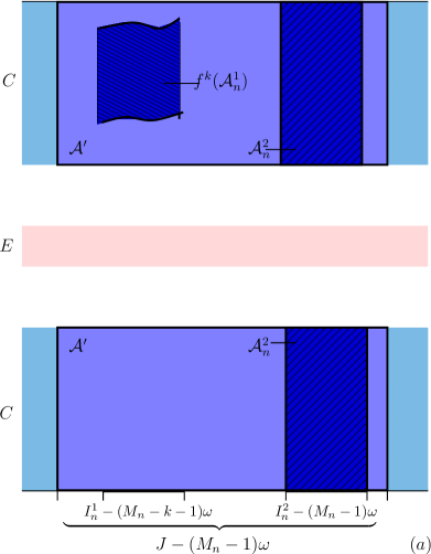
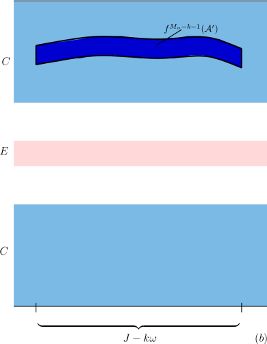
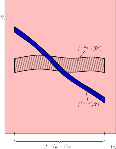
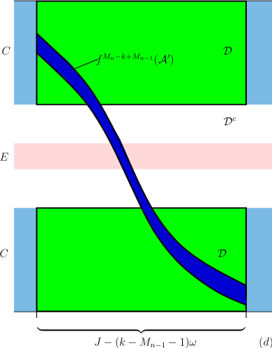
Figure 5.1: Strategy for the proof of Theorem 3.1: The different steps in the forward iteration of $\mathcal{A}^{\prime}$, explaining the creation of the two hooks in Figure 2.1. (a) It suffices to consider the sets $\mathcal{A}^{\prime}$ and $\mathcal{B}^{\prime}$ defined in (5.2), since $\mathcal{A}^{\prime}$ contains $\mathcal{A}^{2}_{n}\cup f^{k}(\mathcal{A}^{1}_{n})$, and similarly $\mathcal{B}^{\prime}$ contains $\mathcal{B}^{1}_{n}\cup f^{-k}(\mathcal{B}^{2}_{n})$ (Lemma 5.3). (b) After $M_{n}-k-1$ iterates, the image of $\mathcal{A}^{\prime}$ is a thin horizontal strip in the contracting region $\mathbb{T}^{1}\times C$. (c) In the next step, it is mapped into the expanding region $\mathbb{T}^{1}\times E$ with negative slope. Therefore it intersects the preimage of the complement of $\mathcal{D}$ under $f^{M_{n-1}}$ in a transveral way. (d) After $M_{n-1}$ further steps, the image of $\mathcal{A}$ is mostly contained in $\mathcal{D}$, but transverses the expanding region in a small interval. Continued in Figure 5.2 … .

The following lemma ensures that it is sufficient to consider $\mathcal{A}^{\prime}$ and $\mathcal{B}^{\prime}$ (instead of the four sets $\mathcal{A}^{1}_{n},\mathcal{A}^{2}_{n},\mathcal{B}^{1}_{n}$ and $\mathcal{B}^{2}_{n}$).

Lemma 5.3.

For all $\tau\in\Gamma$, the following inclusions hold.

(5.3) $$f^{M_{n}}(\mathcal{A}^{2}_{n})\cap f^{-M_{n}}(\mathcal{B}^{2}_{n}) \subseteq f^{M_{n}}(\mathcal{A}^{\prime})\cap f^{-(M_{n}-k)}(\mathcal{B}^{\prime})$$

(5.4) $$f^{k}\left(f^{M_{n}}(\mathcal{A}^{1}_{n})\cap f^{-M_{n}}(\mathcal{B}^{1}_{n})\right) \subseteq f^{M_{n}}(\mathcal{A}^{\prime})\cap f^{-(M_{n}-k)}(\mathcal{B}^{\prime})$$

Hence, in order to apply Proposition 4.7 it will be sufficient to show that $f^{M_{n}}(\mathcal{A}^{\prime})\cap f^{-(M_{n}-k)}(\mathcal{B}^{\prime})=\emptyset$, since in this case both components of $\mathcal{C}_{n}$ are empty.

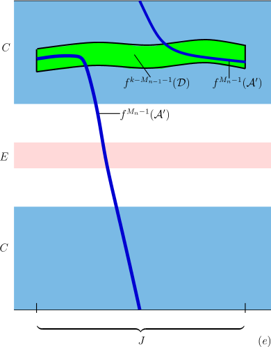
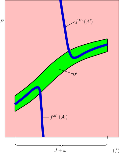
Figure 5.2: Strategy for the proof of Theorem 3.1: (e) After $k-M_{n-1}-1$ more iterates the set $\mathcal{D}$ gets mapped to a thin horizontal strip in the contracting region. (f) In the next step, it gets mapped into the expanding region with positive slope (Lemma 5.6). Due to the relative position of the two sets, this forces the image of $\mathcal{A}^{\prime}$ to develop the two hooks already mentioned in Figure 2.1(b) and (c) (Lemma 5.7).

Next, it will be important to control the geometry of the sets $f^{M_{n}}(\mathcal{A}^{\prime})$ and $f^{-(M_{n}-k)}(\mathcal{B}^{\prime})$. To that end, we introduce the following notation. If $I\subseteq\mathbb{T}^{1}$ is an interval and $A\subseteq\mathbb{T}^{1}$, we denote by $\sup^{I}A$ and $\inf^{I}A$ the supremum, respectively infimum, of $A$ with respect to the natural ordering on $I$, induced by the counter-clockwise orientation on $\mathbb{T}^{1}$. Note that thus $\inf^{I}I$ and $\sup^{I}I$ are the left and right endpoints of $I$. Given $A\subseteq\mathbb{T}^{2}$, $\theta\in\pi_{1}(A)$, we let $A_{\theta}=\{x\in\mathbb{T}^{1}\mid(\theta,x)\in A\}$. If $A_{\theta}$ is an interval for all $\theta\in\pi_{1}(A)$, we define the boundary graphs of $A$ as

$$\varphi^{+}_{A}:\pi_{1}(A)\to\mathbb{T}^{1} \varphi^{+}_{A}(\theta)\ =\ \textstyle\sup^{A_{\theta}}A_{\theta}$$ ,

$$\varphi^{-}_{A}:\pi_{1}(A)\to\mathbb{T}^{1} \varphi^{-}_{A}(\theta)\ =\ \textstyle\inf^{A_{\theta}}A_{\theta}\ .$$ ,

With these notions, we have

Lemma 5.4.

For all $\tau\in\Gamma$, the set $\mathcal{B}^{\prime\prime}=\mathrm{cl}(f_{\tau}^{-(M_{n}-k)}(\mathcal{B}^{\prime}))$ is included in $(J+\omega)\times E$ and satisfies the following.

• $|\mathcal{B}^{\prime\prime}_{\theta}|\ \leq\ |E|\cdot\alpha^{-\frac{M_{n}-k}{p}}$ for all $\theta\in J+\omega$;

• $|\partial_{\theta}\varphi^{\pm}_{\mathcal{B}^{\prime\prime}}(\theta)|\ \leq\ \frac{S}{\alpha^{1/p}-1}$ for all $\theta\in J+\omega$.

Lemma 5.5.

For all $\tau\in\Gamma$, the set $\mathcal{A}^{\prime\prime}=\mathrm{cl}(f_{\tau}^{M_{n}}(\mathcal{A}^{\prime}))$ satisfies the following.

• $|\mathcal{A}^{\prime\prime}_{\theta}|\ \leq\ |C|\cdot\alpha^{-\frac{M_{n}}{p}+(p+\frac{1}{p})k}$ for all $\theta\in J+\omega$;

• $|\partial_{\theta}\varphi^{\pm}_{\mathcal{A}^{\prime\prime}}(\theta)|\ \leq\ \alpha^{pk}\cdot\frac{2S}{1-\alpha^{-p}}$ for all $\theta\in J+\omega$.

Further, the crucial step in the argument will be to control the position of $f^{M_{n}}(\mathcal{A}^{\prime})$ with respect to an intermediate set $\mathcal{D}^{\prime}$ that is defined as follows. Let

(5.5) $$\mathcal{D}\ =\ (J-(k-M_{n-1}-1)\omega)\times C\quad\textrm{and}\quad\mathcal{D}^{\prime}=f^{k-M_{n-1}}(\mathcal{D})\ .$$

Concerning the geometry of $\mathcal{D}^{\prime}$ itself, we have

Lemma 5.6.

For all $\tau\in\Gamma$, the set $\mathcal{D}^{\prime}$ satisfies the following assertions.

• $\mathcal{D}^{\prime}\subseteq(J+\omega)\times E$;

• $|C|\cdot\alpha^{-p(k-M_{n-1})}\ \leq\ |\mathcal{D}^{\prime}_{\theta}|\ \leq\ |C|\cdot\alpha^{-\frac{k-M_{n-1}}{p}}$ for all $\theta\in J+\omega$;

• $s-\frac{S}{\alpha^{1/p}-1}\ \leq\ \partial_{\theta}\varphi^{\pm}_{\mathcal{D}^{\prime}}(\theta)\ \leq\ S+\frac{S}{\alpha^{1/p}-1}$ for all $\theta\in J+\omega$.

Now, the following statements yield the required information about the relations between $\mathcal{D}^{\prime}$ and $f^{M_{n}}(\mathcal{A}^{\prime})$.

Lemma 5.7.

For all $\tau\in\Gamma$ there exists an open interval $P_{0}\subseteq J+\omega$ of length between $\frac{1-|C|}{4S}\cdot\alpha^{-pM_{n-1}}$ and $\frac{4(1-|C|)}{s}\cdot\alpha^{-M_{n-1}/p}$ such that $\pi_{1}(\mathcal{A}^{\prime\prime}\cap\mathcal{D}^{\prime})=(J+\omega)\setminus P_{0}$. Moreover, $\mathcal{A}^{\prime\prime}$ leaves and enters $\mathcal{D}^{\prime}$ in the clockwise direction at the endpoints of $P_{0}$ and the boundary curves of $\mathcal{A}^{\prime\prime}$ intersect those of $\mathcal{D}^{\prime}$ exactly once. Further, $P_{0}\cap(I_{n}^{1}+(k+1)\omega)\neq\emptyset$.

Lemma 5.8.

There exists an arc $\Xi=\{(\theta,\xi(\theta))\mid\theta\in J+\omega\}\subseteq(J+\omega)\times C$, with continuous $\xi:J+\omega\to C$, such that $P_{1}=\pi_{1}(\mathcal{A}^{\prime\prime}\cap\Xi)$ is an interval.

Remark 5.9.

Note that since $\mathcal{D}^{\prime}\subseteq(J+\omega)\times E$, $|\mathcal{A}_{\theta}^{\prime\prime}|\leq\alpha^{-\frac{M_{n}}{p}+(p+\frac{1}{p})k}$ and $d(C,E)>\alpha^{-\frac{M_{n}}{p}+(p+\frac{1}{p})k}$ if $n\in\mathbb{N}$ is sufficiently large, we have that $P_{1}\subseteq P_{0}$. From now on, we always assume that this is the case. Moreover, as the slope of $\partial_{\theta}\varphi_{\mathcal{A}^{\prime\prime}}^{\pm}(\theta)$ is smaller than $\alpha^{pk}\cdot\frac{2S}{1-\alpha^{-p}}$, we obtain

(5.6) $$d(P_{1},\mathbb{T}^{1}\setminus P_{0})\ \geq\ \frac{d(C,E)-2\alpha^{-\frac{M_{n}}{p}+(p+\frac{1}{p})k}}{\alpha^{p(k+1)}\cdot\frac{2S}{\alpha^{p}-1}}\ \geq\ d(C,E)\cdot\alpha^{-p(k+1)}/2\ \geq\ \alpha^{-2pk}\ ,$$

where the last inequality again requires that $n$ (and thus $k\geq M_{n-1}$) is sufficiently large.

Denote by $J^{-}$ and $J^{+}$ the left, respectively right component of $(J+\omega)\setminus P_{0}$. Define

$$\mathcal{L}_{1} = \{(\theta,x)\mid\theta\in J^{-},x\in[e^{-},\varphi^{+}_{\mathcal{D}^{\prime}}(\theta)]\}$$

$$\mathcal{R}_{1} = \{(\theta,x)\mid\theta\in J^{+},x\in[\varphi^{-}_{\mathcal{D}^{\prime}}(\theta),e^{+}]\}\ .$$

Further, denote by $P_{0}^{-}$ and $P_{0}^{+}$ the left, respectively right component of $P_{0}\setminus\mathrm{int}(P_{1})$. Define

$$\mathcal{L}_{2} = \{(\theta,x)\mid\theta\in P_{0}^{-},x\in[e^{-},\varphi^{-}_{\mathcal{D}^{\prime}}(\theta)]\}$$

$$\mathcal{R}_{2} = \{(\theta,x)\mid\theta\in P_{0}^{+},x\in[\varphi^{+}_{\mathcal{D}^{\prime}}(\theta),e^{+}]\}\ .$$

Let $\mathcal{L}=\mathcal{L}_{1}\cup\mathcal{L}_{2}$ and $\mathcal{R}=\mathcal{R}_{1}\cup\mathcal{R}_{2}$. (See Figure 5.3 for an illustration.)

Remark 5.10.

We have $\mathcal{A}^{\prime\prime}\cap\left(\ (J+\omega)\ \times E\right)\subseteq\mathcal{L}\cup\mathcal{R}$ if $\alpha$ and $n$ are large.

Proof.

Note that since $\Xi\subseteq(J+\omega)\times C$ and $|\mathcal{A}^{\prime\prime}_{\theta}|\leq\alpha^{-\frac{M_{n}}{p}+(p+\frac{1}{p})k}<d(C,E)$ (using $k\ll M_{n}$ and assuming $\alpha$ to be large), we have $\mathcal{A}^{\prime\prime}\cap(P_{1}\times E)=\emptyset$. Moreover, $\mathcal{A}^{\prime\prime}$ only crosses the arc $\Xi$ once. The statement therefore follows from the way $\mathcal{A}^{\prime\prime}$ leaves and enters $\mathcal{D}^{\prime}\subseteq(J+\omega)\times E$, according to Lemma 5.7. ∎

Finally, the following statement ensures that at the extremal points of $\Gamma$, different situations occur.

Lemma 5.11.

At $\tau=\tau^{-}$, the set $\mathcal{B}^{\prime\prime}$ intersects $\mathcal{R}$, whereas at $\tau=\tau^{+}$ it intersects $\mathcal{L}$.

Based on the above statements, we can now turn to the proof of Theorem 3.1, which is illustrated in Figure 5.3.

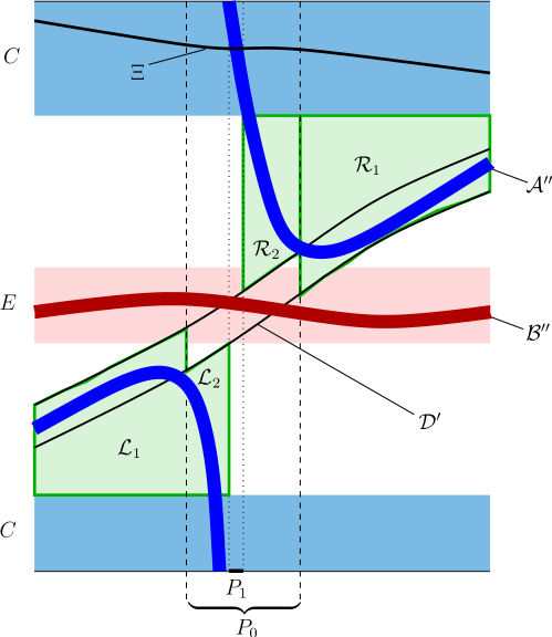
Figure 5.3: Illustration of the different sets considered in the proof of Theorem 3.1.

Proof of Theorem 3.1..

Suppose $\omega\in\mathcal{D}(\gamma,\nu)$ and $\hat{f}\in\mathcal{P}_{\omega}$ satisfies conditions (${\cal A}1$)–($\mathcal{A}10$). Fix $\delta>0$, denote by $\alpha_{*}^{\prime},\varepsilon_{*}^{\prime}>0$ the constants given by Theorem 4.1 and recall that $q\geq\max\{8,4\nu\}$. We have to show that for any parameter $\tau_{0}$ contained in the set $\Lambda^{\hat{f}}$ from Theorem 4.1 and any $\zeta>0$ there exists some $\tau\in B_{\zeta}(\tau_{0})$ such that $f_{\tau}$ is mode-locked, provided that $\alpha>\alpha^{\prime}_{*}$ is sufficiently large and $\varepsilon_{0}<\varepsilon^{\prime}_{*}$ is sufficiently small. The largeness and smallness assumptions on $\alpha$ and $\varepsilon_{0}$ will be used implicitely from now on, and all estimates below should be understood under this premise.

To that end, fix $\tau_{0}\in\Lambda^{\hat{f}}$ and $\zeta>0$. Choose $n\in\mathbb{N}$ and $\Gamma=[\tau^{-},\tau^{+}]\subseteq B_{\zeta}(\tau_{0})$ according to Lemma 5.1. By Proposition 4.7, it suffices to find some $\tau\in\Gamma$ such that $\mathcal{C}_{n}=\emptyset$. Moreover, due to Lemma 5.3, this follows if we can show that

(5.7) $$f^{M_{n}}_{\tau}(\mathcal{A}^{\prime})\cap f_{\tau}^{-(M_{n}-k)}(\mathcal{B}^{\prime})\ =\ \mathcal{A}^{\prime\prime}\cap\mathcal{B}^{\prime\prime}\ =\ \emptyset\ .$$

Due to Lemma 5.4, we know that $\mathcal{B}^{\prime\prime}\subseteq(J+\omega)\times E$, and we have $\mathcal{A}^{\prime\prime}\cap((J+\omega)\times E)\subseteq\mathcal{L}(\tau)\cup\mathcal{R}(\tau)$ by Remark 5.10. We claim that for all $\tau\in\Gamma$ the strip $\mathcal{B}^{\prime\prime}$ can intersect at most one of the two sets $\mathcal{L}$ and $\mathcal{R}$. Since it intersects $\mathcal{R}$ for $\tau=\tau^{-}$ and $\mathcal{L}$ for $\tau=\tau^{+}$ by Lemma 5.11 and all sets are closed and depend continuously on $\tau$, this means that for some $\tau\in(\tau^{-},\tau^{+})$ we must have $f_{\tau}^{-(M_{n}-k)}(\mathcal{B}^{\prime})\cap(\mathcal{L}(\tau)\cup\mathcal{R}(\tau))=\emptyset$. This, in turn, yields (5.7) and thus completes the proof.

Hence, it remains to show that $\mathcal{B}^{\prime\prime}$ cannot intersect both $\mathcal{L}$ and $\mathcal{R}$ at the same time. Suppose for a contradiction that $(\theta_{1},x_{1})\in\mathcal{B}^{\prime\prime}\cap\mathcal{L}$ and $(\theta_{2},x_{2})\in\mathcal{B}^{\prime\prime}\cap\mathcal{R}$. By Lemma 5.4, we have

(5.8) $$x_{2}-x_{1}\ \leq\ \frac{S}{\alpha^{1/p}-1}\cdot|\theta_{2}-\theta_{1}|+|E|\cdot\alpha^{-\frac{M_{n}-k}{p}}\ .$$

We distinguish four cases. Thereby, we will use freely the fact that $\alpha$ is sufficiently large and indicate when this is used by placing $(\alpha)$ over the respective inequality signs.

Case I

Suppose $(\theta_{1},x_{1})\in\mathcal{L}_{1}$ and $(\theta_{2},x_{2})\in\mathcal{R}_{1}$. In this case, we have that

(5.9) $$\theta_{2}-\theta_{1}\ \geq\ |P_{0}|\ \geq\ \frac{1-|C|}{4S}\cdot\alpha^{-pM_{n-1}}$$

by Lemma 5.7 and

$$x_{2}-x_{1} \geq \varphi^{-}_{\mathcal{D}^{\prime}}(\theta_{2})-\varphi^{+}_{\mathcal{D}^{\prime}}(\theta_{1})$$

$$\stackrel{{\scriptstyle\textrm{Lem.\leavevmode\nobreak\ \ref{l.D_shape}(ii)}}}{{\geq}} \ \varphi^{-}_{\mathcal{D}^{\prime}}(\theta_{2})-\varphi^{-}_{\mathcal{D}^{\prime}}(\theta_{1})-\alpha^{-\frac{k-M_{n-1}}{p}}$$

$$\stackrel{{\scriptstyle\textrm{Lem.\leavevmode\nobreak\ \ref{l.D_shape}(iii)}}}{{\geq}} \frac{s}{2}\cdot(\theta_{2}-\theta_{1})-\alpha^{-\frac{k-M_{n-1}}{p}}$$

$$\ \stackrel{{\scriptstyle(\ref{eq:12}),(\alpha)}}{{\geq}} \frac{S}{\alpha^{1/p}-1}\cdot(\theta_{2}-\theta_{1})+\alpha^{-\frac{M_{n}-k}{p}}\ ,$$

contradicting (5.8).

Case II

Suppose $(\theta_{1},x_{1})\in\mathcal{L}_{1}$ and $(\theta_{2},x_{2})\in\mathcal{R}_{2}$. In this case, we have

(5.10) $$\theta_{2}-\theta_{1}\ \geq\ d(P_{1},\mathbb{T}^{1}\setminus P_{0})\ \geq\alpha^{-2pk}$$

by Remark 5.9. Moreover, the definitions of $\mathcal{L}_{1}(\tau)$ and $\mathcal{R}_{2}(\tau)$ imply that

$$x_{2}-x_{1} \geq \varphi^{+}_{\mathcal{D}^{\prime}}(\theta_{2})-\varphi^{+}_{\mathcal{D}^{\prime}}(\theta_{1})$$

$$\stackrel{{\scriptstyle\textrm{Lemma\leavevmode\nobreak\ \ref{l.D_shape}(iii)},(\alpha)}}{{\geq}} \frac{s}{2}\cdot(\theta_{2}-\theta_{1})\ \stackrel{{\scriptstyle(\ref{eq:11}),(\alpha)}}{{\geq}}\ \frac{S}{\alpha^{1/p}-1}\cdot(\theta_{2}-\theta_{1})+\alpha^{-\frac{M_{n}-k}{p}}\ ,$$

again contradicting (5.8).

Case III

The case $(\theta_{1},x_{1})\in\mathcal{L}_{2}$ and $(\theta_{2},x_{2})\in\mathcal{R}_{1}$ is symmetric to the preceeding one and can be treated in the same way.

Case IV

Finally, suppose $(\theta_{1},x_{1})\in\mathcal{L}_{2}(\tau)$ and $(\theta_{2},x_{2})\in\mathcal{R}_{2}(\tau)$. In this case

$$x_{2}-x_{1} \geq \varphi^{+}_{\mathcal{D}^{\prime}}(\theta_{2})-\varphi^{-}_{\mathcal{D}^{\prime}}(\theta_{1})$$

$$\stackrel{{\scriptstyle\textrm{Lemma\leavevmode\nobreak\ \ref{l.D_shape}}(ii)}}{{\geq}} \varphi^{+}_{\mathcal{D}^{\prime}}(\theta_{2})-\varphi^{+}_{\mathcal{D}^{\prime}}(\theta_{1})+|C|\cdot\alpha^{-p(k-M_{n-1})}$$

$$\stackrel{{\scriptstyle\textrm{Lemma\leavevmode\nobreak\ \ref{l.D_shape}}}}{{\geq}} \frac{s}{2}\cdot(\theta_{2}-\theta_{1})+|C|\cdot\alpha^{-p(k-M_{n-1})}$$

$$\stackrel{{\scriptstyle(\alpha)}}{{\geq}} \frac{S}{\alpha^{1/p}-1}\cdot(\theta_{2}-\theta_{1})+\alpha^{-\frac{M_{n}-k}{p}}\ ,$$

contradicting (5.8) as before. ∎

6 Proofs of the geometric estimates

Throughout the proofs of this section, we will at most times omit the parameter $\tau$ from the notation and write $f$, $f_{\theta}$ and $I^{\iota}_{n}$ instead of $f_{\tau}$, $f_{\tau,\theta}$ and $I^{\iota}_{n}(\tau)$ (with the exception of the proof of Lemma 5.1). Moreover, we will always assume implicitely that the parameter $\alpha$ is sufficiently large and $\varepsilon_{0}$ is sufficiently small. All estimates below should be understood in this sense. Sometimes, but not always, we will indicate that this fact is used by placing $(\alpha)$ or $(\varepsilon_{0})$ over the respective inequality signs.

6.1 Proof of Lemma 5.1.

According to (4.3) and (4.4), there exists some $n\in\mathbb{N}$, $n\geq 10$, so that $\frac{s}{4L}\varepsilon_{n-1}<\zeta$. We fix this $n$ and first prove that there exists some $k\in\left[2K_{n-1}M_{n-1}+1,\ M_{n-1}^{4q(\nu+1)}\right]$, such that

(6.1) $$d\left(I_{n}^{1}(\tau_{0})+k\omega,I_{n}^{2}(\tau_{0})\right)\ <\ \frac{s\ell}{8LS}\varepsilon_{n-1}$$

and $I_{n}^{1}(\tau_{0})+k\omega$ is to the left of $I_{n}^{2}(\tau_{0})$ in a local sense. Since $(\mathcal{X})_{n-1}$ holds for $\tau_{0}$, it is obvious that $k\geq 2K_{n-1}M_{n-1}+1$.

For any $N\in\mathbb{N}$, there is a positive integer $m\leq N$ such that $d(m\omega,0)\leq\frac{1}{N}$. Moreover, since $\omega$ is Diophantine, we have $d(m\omega,0)\geq\gamma m^{-\nu}\geq\gamma N^{-\nu}$. Together, this implies that after $N\left([\gamma^{-1}N^{\nu}]+1\right)$ iterates, the orbit of $\omega$ is $\frac{1}{N}$ dense in the circle. Thus, there exists some $k\leq N\left([\gamma^{-1}N^{\nu}]+1\right)\leq 2\gamma^{-1}N^{\nu+1}$ such that $d\left(I_{n}^{1}(\tau_{0})+k\omega,I_{n}^{2}(\tau_{0})\right)\leq 1/N$ and $I_{n}^{1}(\tau_{0})+k\omega$ is to the left of $I_{n}^{2}(\tau_{0})$. Taking $N=\left[\frac{4LS}{\ell}\alpha^{M_{n-2}/p}\right]+1$, we obtain

$$d(I_{n}^{1}(\tau_{0})+k\omega,I_{n}^{2}(\tau_{0}))\ <\ \frac{\ell}{4LS}\alpha^{-M_{n-2}/p}\ \stackrel{{\scriptstyle(\ref{e.eps_j})}}{{\leq}}\ \frac{s\ell}{8LS}\varepsilon_{n-1}\$$

and

$$k \leq \frac{2}{\gamma}\left(\frac{4LS}{\ell}\alpha^{M_{n-2}/p}+1\right)^{\nu+1}$$

$$\stackrel{{\scriptstyle(\ref{e.M_j})}}{{\leq}} \frac{2}{\gamma}\left(\frac{4LS}{\ell}M_{n-1}^{2q}+1\right)^{\nu+1}\ \stackrel{{\scriptstyle(\alpha)}}{{\leq}}\ M_{n-1}^{4q(\nu+1)}\ \stackrel{{\scriptstyle(\alpha)}}{{\ll}}\ M_{n}\ .$$

We now claim that conditions $(\mathcal{X})_{n-1}$ and $(\mathcal{Y}^{\prime\prime})_{n}$ are satisfied for all $\tau$ with $|\tau-\tau_{0}|<\frac{s}{4L}\varepsilon_{n-1}$. In order to do so, we proceed by induction on $j$. Suppose that $(\mathcal{X})_{j-1}$ and $(\mathcal{Y}^{\prime\prime})_{j-1}$ hold for $\tau\in B_{\frac{s}{4L}\varepsilon_{n-1}}(\tau_{0})$. Then we have $|I_{j}^{\iota}(\tau)|\leq\varepsilon_{j}$ and $|\partial_{\tau}I_{j}^{\iota}(\tau)|\leq\frac{2L}{s}$, $\iota=1,2,$ by Proposition 4.6 if $j\geq 1$ and by assumption if $j=0$. If $d_{H}$ denotes the Hausdorff distance, then this implies that $d_{H}(I_{j}^{\iota}(\tau),I_{j}^{\iota}(\tau_{0})\leq\frac{2L}{s}\cdot|\tau-\tau_{0}|$.

Thus, using $(\mathcal{X}^{\prime})_{j}$ for $\tau_{0}$, we have for all $l=1,\ldots,2K_{j}M_{j}$ and $\iota_{1},\iota_{2}=1,2,$

$$d(I_{j}^{\iota_{1}}(\tau),I_{j}^{\iota_{2}}(\tau)+l\omega)$$

$$\geq d(I_{j}^{\iota_{1}}(\tau_{0}),I_{j}^{\iota_{2}}(\tau_{0})+l\omega)-d_{H}(I_{j}^{\iota_{1}}(\tau_{0}),I_{j}^{\iota_{1}}(\tau))-d_{H}(I_{j}^{\iota_{2}}(\tau_{0})+l\omega,I_{j}^{\iota_{2}}(\tau)+l\omega)$$

$$> 9\varepsilon_{j}-\frac{2L}{s}\cdot\frac{s\varepsilon_{n-1}}{4L}-\frac{2L}{s}\cdot\frac{s\varepsilon_{n-1}}{4L}\ >\ 3\varepsilon_{j}\$$

if $j\leq n-1$. Hence, $(\mathcal{X})_{j}$ holds for $\tau$. In a similar way, using $(\mathcal{Y}^{\prime})_{j}$ for $\tau_{0}$, we have that for $\iota_{1},\iota_{2}=1,2,\ j\leq n,\ 0\leq j^{\prime}\leq j-1,$ and $-M_{j^{\prime}}\leq l\leq M_{j^{\prime}}+2$

$$d(I_{j}^{\iota_{1}}(\tau)-(M_{j}-1)\omega,I_{j^{\prime}}^{\iota_{2}}(\tau)+l\omega)\ >\ \varepsilon_{j-1}\ ,$$

and

$$d(I_{j}^{\iota_{1}}(\tau)+(M_{j}+1)\omega,I_{j^{\prime}}^{\iota_{2}}(\tau)+l\omega)\ >\ \varepsilon_{j-1}\ ,$$

as long as $j\leq n$. Therefore, conditions $(\mathcal{X})_{n-1}$ and $(\mathcal{Y}^{\prime\prime})_{n}$ hold for $\tau\in B_{\frac{s}{4L}\varepsilon_{n-1}}(\tau_{0})$ as claimed.

Now, due to (4.13) the interval $I^{1}_{n}(\tau)+k\omega$ moves with positive minimal speed $\ell/S$ relative to $I^{2}_{n}(\tau)$. Hence, it follows from (6.1) that $I^{1}_{n}(\tau)+k\omega$ moves from the left to the right of $I_{n}^{2}(\tau)$ when $\tau$ transverses the interval $[\tau_{0},\tau_{0}+\frac{s}{4L}\varepsilon_{n-1}]$. (note that $|I^{\iota}_{n}(\tau)|\leq\varepsilon_{n}$ by Proposition 4.6 and $\varepsilon_{n}\ll\varepsilon_{n-1}$). Thus, we can choose a subinterval $\Gamma=[\tau^{-},\tau^{+}]\subseteq[\tau_{0},\tau_{0}+\frac{s}{4L}\varepsilon_{n-1}]$ that satisfies all the assertions of the lemma.∎

6.2 Proof of Lemma 5.3

We first need the following statement.

Claim 6.1.

Let $\Gamma$ be as in Lemma 5.1. Then for all $\tau\in\Gamma$ the following statement holds.

(6.2) $$(J+l\omega)\cap\mathcal{I}_{n}=\emptyset,\ \ \ \ \forall\ \ l\in\{-M_{n}-k+1,\ldots,M_{n}+1\}\setminus\{-k,0\}.$$

Proof.

By Lemma 5.1, we have $k\leq M_{n-1}^{4q(\nu+1)}\ll M_{n}$ for $\alpha$ large, and conditions $(\mathcal{X})_{n-1},(\mathcal{Y}^{\prime\prime})_{n-1}$ hold for all $\tau\in\Gamma$. Proposition 4.6, implies $|I_{n}^{\iota}|\leq\varepsilon_{n},\ \iota=1,2$. Suppose $l\in\{-M_{n}-k+1,\ldots,M_{n}+1\}\setminus\{-k,0\}$. Then $\omega\in\mathcal{D}(\gamma,\nu)$, (4.3) and (4.4) yield

$$d(I_{n}^{1}+(k+l)\omega,I_{n}^{1})\geq d((k+l)\omega,0)-|I_{n}^{1}|$$

$$\geq \gamma\cdot|k+l|^{-\nu}-\varepsilon_{n}\ >\ \gamma\cdot(2M_{n})^{-\nu}-\varepsilon_{n}\ \stackrel{{\scriptstyle(\alpha)}}{{>}}\ 9\varepsilon_{n}\$$

and

$$d(I_{n}^{2}+l\omega,I_{n}^{2})\geq d(l\omega,0)-|I_{n}^{2}|$$

$$\geq \gamma\cdot|l|^{-\nu}-\varepsilon_{n}\ >\ \gamma\cdot(2M_{n})^{-\nu}-\varepsilon_{n}\ \stackrel{{\scriptstyle(\alpha)}}{{>}}\ 9\varepsilon_{n}\ .$$

Since $J\subseteq B_{9\varepsilon_{n}}(I_{n}^{1}+k\omega)\cap B_{9\varepsilon_{n}}(I_{n}^{2})$, this implies (6.2). ∎

Now we can turn to the proof of Lemma 5.3. Since $I_{n}^{2}\cup(I_{n}^{1}+k\omega)\subseteq J$, we have that $\mathcal{A}_{n}^{2}\subseteq\mathcal{A}^{\prime}$ and $\mathcal{B}_{n}^{1}\subseteq\mathcal{B}^{\prime}$ by definition. Thus, it will be sufficient to show that

$$f^{-k}(\mathcal{B}_{n}^{2})\ \subseteq\ \mathcal{B}^{\prime}\ \ \textrm{and}\ \ f^{k}(\mathcal{A}_{n}^{1})\ \subseteq\ \mathcal{A}^{\prime}.$$

As for $\mathcal{B}_{n}^{2}$, we have $\left(I_{n}^{2}+(M_{n}+1)\omega\right)\cap\mathcal{V}_{n-1}^{+}=\emptyset$ by condition $(\mathcal{Y}^{\prime\prime})_{n}$. Moreover, $(\mathcal{Y}^{\prime\prime})_{n}$ together with $d(I_{n}^{1}+(M_{n}+1)\omega,I_{n}^{2}+(M_{n}-k+1)\omega)\leq 4\varepsilon_{n}\ll\varepsilon_{n-1}$ yields $(I_{n}^{2}+(M_{n}-k+1)\omega)\cap\mathcal{W}_{n-1}^{+}=\emptyset$. Moreover, due to Claim 6.1 we have that $k$ is the first integer such that $J-k\omega$ intersects $\mathcal{I}_{n}$. Thus, we can apply Lemma 4.4 to obtain $f^{-k}(\mathcal{B}_{n}^{2})\subseteq\mathcal{B}^{\prime}$.

Similarly, we have $\left(I_{n}^{1}-(M_{n}-1)\omega\right)\cap\mathcal{V}_{n-1}^{-}=\emptyset$ by $(\mathcal{Y}^{\prime\prime})_{n}$, and the fact that $d(I_{n}^{2}-(M_{n}-1)\omega,I_{n}^{1}-(M_{n}-k-1)\omega)\leq 4\varepsilon_{n}\ll\varepsilon_{n-1}$ together with $(\mathcal{Y}^{\prime\prime})_{n}$ also imply $(I_{n}^{1}-(M_{n}-k-1)\omega)\cap\mathcal{W}^{+}_{n-1}=\emptyset$. Thus Claim 6.1 combined with Lemma 4.3 yield $f^{k}(\mathcal{A}_{n}^{1})\subseteq\mathcal{A}^{\prime}$. ∎

6.3 Proof of Lemma 5.4

For the proof, we first need the following statement.

Claim 6.2.

Let $\hat{f}$ satisfy the assertion of Theorem 4.1 and assume $\tau\in\Lambda_{n-1}^{\hat{f}}$. Then for $n\geq 3$, we have

(6.3) $$f^{M_{n-1}}(\mathcal{A}_{n-1}^{\iota})\subseteq\mathbb{T}^{1}\times E,\ \ \iota=1,2,$$

(6.4) $$B_{9\varepsilon_{n}}(I_{n}^{\iota})\subseteq I_{n-1}^{\iota},\ \ \iota=1,2.$$

Proof.

The proof is illustrated in Figure 6.1. We let

$$I_{j}^{\iota}=(a_{j}^{\iota},b_{j}^{\iota}),\ \ \tilde{\mathcal{A}}_{j}^{\iota}=f^{M_{j}}(\mathcal{A}_{j}^{\iota}),\ \ \hat{\mathcal{B}}_{j}^{\iota}=f^{-M_{j}}(\mathcal{B}_{j}^{\iota}),\ \ \iota=1,2,\ j=0,1,\ldots,n-1.$$

We have $\mathcal{I}_{j}-(M_{j}-1)\omega\cap\mathcal{V}^{-}_{j-1}=\emptyset$ and $\mathcal{I}_{j}-(M_{j-1}-1)\omega\cap\mathcal{W}^{+}_{j-1}=\emptyset$ for all $j=0,\ldots,n-1$ by $(\mathcal{Y})_{n-1}$. Hence, Lemma 4.3 yields $f^{M_{j}-M_{j-1}}(\mathcal{A}^{\iota}_{j})\subseteq\mathcal{A}^{\iota}_{j-1}$ for all $j=0,\ldots,n-1$ and therefore $\tilde{\mathcal{A}}^{\iota}_{n-1}\subseteq\tilde{\mathcal{A}}^{\iota}_{n-2}\subseteq\ldots\subseteq\tilde{\mathcal{A}}_{2}^{\iota}$. Thus, it suffices to prove (6.3) for the case $n=3$.

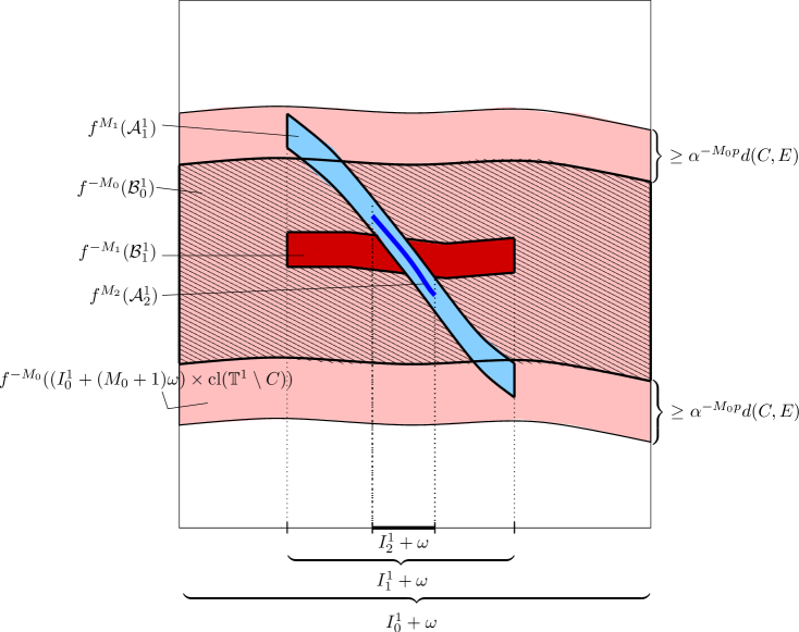
Figure 6.1: Proof of the inclusion (6.3) in Claim 6.2: Position of $f^{M_{2}}(\mathcal{A}_{2}^{1})$. Since this set is close to $f^{-M_{1}}(\mathcal{B}^{1}_{1})$, which lies well inside the expanding region, we obtain $f^{M_{2}}(\mathcal{A}_{2}^{1})\subseteq\mathbb{T}^{1}\times E$ as well.

A similar argument with Lemma 4.4 for the backwards iteration yields $f^{-(M_{1}-M_{0})}(\mathcal{B}^{\iota}_{1})\subseteq\mathcal{B}^{\iota}_{0}$. Since $f^{-M_{0}}(\mathcal{B}^{\iota}_{0})\subseteq f^{-M_{0}}((I^{\iota}_{0}+(M_{0}+1)\omega)\times\textrm{cl}(\mathbb{T}^{1}\setminus C))\subseteq\mathbb{T}^{1}\times E$ by (${\cal A}1$) and $(\mathcal{X})_{0}$, we can use (${\cal A}2$) to obtain

$$d(\mathbb{T}^{1}\setminus E,\hat{\mathcal{B}}_{1,\theta}^{\iota})\ \geq\ \alpha^{-M_{0}p}d(C,E)$$

for all $\theta\in I^{\iota}_{1}+\omega$ (see Figure 6.1). Moreover, by Lemma 4.8, we have that

$$|\varphi_{\tilde{\mathcal{A}}_{1}^{\iota}}^{+}(\theta)-\varphi_{\tilde{\mathcal{A}}_{1}^{\iota}}^{-}(\theta)|\ \leq\ \alpha^{-M_{1}/p}|C|\ \stackrel{{\scriptstyle(\alpha)}}{{<}}\ \alpha^{-M_{0}p}d(E,C)\ .$$

Therefore, by definition of $I^{\iota}_{2}=\mathrm{int}\left(\pi_{1}\left(\hat{\mathcal{B}}^{\iota}_{1}\cap\tilde{\mathcal{A}}^{\iota}_{1}\right)\right)$, this yields

$$f^{M_{2}}(\mathcal{A}_{2}^{\iota})\ \subseteq\ f^{M_{1}}\left((I_{2}^{\iota}-(M_{1}-1)\omega)\times C\right)\subseteq\mathbb{T}^{1}\times E\ .$$

This proves (6.3).

As for (6.4), we first consider the case $\iota=1$ and verify that ${\tilde{\mathcal{A}}}_{j}^{1}$ ‘crosses’ ${\hat{\mathcal{B}}}_{j}^{1}$ ‘downwards’ for all $j=0,1,\ldots,n-1$. Since $(I_{j}^{1}-(M_{j}-1)\omega)\cap\mathcal{V}_{j-1}^{-}=\emptyset,I_{j}^{1}\subseteq\mathcal{I}_{j-1}$ and $\forall\ l=0,1,\ldots,M_{j}-2,(I_{j}^{1}-(M_{j}-1-l)\omega)\cap\mathcal{I}_{j}=\emptyset$ for all $j=0,1,\ldots,n-1$ by $(\mathcal{X})_{n-1},(\mathcal{Y})_{n-1}$, Lemma 4.8 implies that

$$-S-\frac{S}{\alpha^{1/p}-1}\ \leq\ \partial_{\theta}\varphi_{\tilde{\mathcal{A}}_{j}^{1}}^{\pm}(\theta)\ <\ -s+\frac{S}{\alpha^{1/p}-1}.$$

A similar argument with Lemma 4.9 for the backwards iteration yields

$$|\partial_{\theta}\varphi_{\hat{\mathcal{B}}_{j}^{1}}^{\pm}(\theta)|\leq\frac{S}{\alpha^{1/p}-1},\ \ \forall\ j=0,1,\ldots,n-1.$$

Therefore, for any $\iota_{1},\iota_{2}\in\{\pm\},j=0,1,\ldots,n-1$, we have

• $-2S\stackrel{{\scriptstyle(\alpha)}}{{<}}-S-\frac{2S}{\alpha^{1/p}-1}\leq\partial_{\theta}(\varphi_{\tilde{\mathcal{A}}_{j}^{1}}^{\iota_{1}}(\theta)-\varphi_{\hat{\mathcal{B}}_{j}^{1}}^{\iota_{2}}(\theta))\leq-s+\frac{2S}{\alpha^{1/p}-1}\stackrel{{\scriptstyle(\alpha)}}{{<}}-s/2.$

Moreover, $\tilde{\mathcal{A}}_{0}^{1}$ is above $\hat{\mathcal{B}}_{0}^{1}$ at the left end of $I_{0}^{1}+\omega$ and below at the right end by (${\cal A}6$) and (${\cal A}7$), since $\tilde{\mathcal{A}}_{0}^{1}\subseteq f(I_{0}^{1}\times C)$ and $\hat{\mathcal{B}}_{0}^{1}\subseteq(I_{0}^{1}+\omega)\times E$ by (${\cal A}1$) and $(\mathcal{X})_{0}$. Since $\tilde{\mathcal{A}}_{n-1}^{1}\subseteq\cdots\subseteq\tilde{\mathcal{A}}_{0}^{1}$ and $\hat{\mathcal{B}}_{n-1}^{1}\subseteq\cdots\subseteq\hat{\mathcal{B}}_{0}^{1}$ by $(\mathcal{X})_{n-1},(\mathcal{Y})_{n-1}$ and Lemma 4.3, 4.4, the definition of $I_{j}^{1}$ yields

• $\tilde{\mathcal{A}}_{j}^{1}$ is above $\hat{\mathcal{B}}_{j}^{1}$ at the left end of $I_{j}^{1}+\omega$ and below at the right end. (see Figure 6.2)

Thus, (i) and (ii) ensure that $\tilde{\mathcal{A}}_{j}^{1}$ ‘crosses’ $\hat{\mathcal{B}}_{j}^{1}$ ‘downwards’ (and give a precise meaning to this statement). Hence, by definition of $I_{j+1}^{1}$, we have

(6.5) $$\varphi_{\tilde{\mathcal{A}}_{j}^{1}}^{-}(a_{j+1}^{1}+\omega)-\varphi_{\hat{\mathcal{B}}_{j}^{1}}^{+}(a_{j+1}^{1}+\omega)=0,\ \ j=0,1,\ldots,n-1,$$

(6.6) $$\varphi_{\tilde{\mathcal{A}}_{j}^{1}}^{+}(b_{j+1}^{1}+\omega)-\varphi_{\hat{\mathcal{B}}_{j}^{1}}^{-}(b_{j+1}^{1}+\omega)=0,\ \ j=0,1,\ldots,n-1\ .$$

Further, we have $(I_{n-1}^{1}-(M_{n-1}-1)\omega)\cap\mathcal{V}_{n-2}^{-}=\emptyset$ and $(I_{n-1}-M_{n-2}\omega)\cap\mathcal{W}^{+}_{n-2}=\emptyset$ by $(\mathcal{Y})_{n-1}$, so that Lemma 4.3 implies $f^{M_{n-1}-M_{n-2}-1}(\mathcal{A}_{n-1}^{1})\subseteq\mathbb{T}^{1}\times C$. Moreover, since $(I_{n-1}^{1}-M_{n-2}\omega)\cap\mathcal{I}_{0}=\emptyset$ by $(\mathcal{Y})_{n-1}$, we also have $f((I_{n-1}^{1}-M_{n-2}\omega)\times\textrm{cl}(\mathbb{T}^{1}\setminus E))\subseteq\mathbb{T}^{1}\times C$. Thus, for $\theta\in I_{n-1}^{1}+\omega$,

$$|f_{\theta-M_{n-1}\omega}^{M_{n-1}-M_{n-2}}(c^{\pm})-c^{\pm}|\geq\alpha^{-p}d(C,E).$$

Combined with (${\cal A}2$) this means that if $\theta\in I_{n-1}^{1}+\omega$, then

$$|\varphi_{\tilde{\mathcal{A}}_{n-1}^{1}}^{\pm}(\theta)-\varphi_{\tilde{\mathcal{A}}_{n-2}^{1}}^{\pm}(\theta)|\ =\ |f_{\theta-M_{n-2}\omega}^{M_{n-2}}(f_{\theta-M_{n-1}\omega}^{M_{n-1}-M_{n-2}}(c^{\pm}))-f_{\theta-M_{n-2}\omega}^{M_{n-2}}(c^{\pm})|$$

$$\geq \alpha^{-pM_{n-2}}|f_{\theta-M_{n-1}\omega}^{M_{n-1}-M_{n-2}}(c^{\pm})-c^{\pm}|\ \geq\alpha^{-p(M_{n-2}+1)}d(C,E).$$

Similarly, given $\theta\in I_{n-1}^{1}+\omega$ we have

$$|\varphi_{\hat{\mathcal{B}}_{n-1}^{\iota}}^{\pm}(\theta)-\varphi_{\hat{\mathcal{B}}_{n-2}^{\iota}}^{\pm}(\theta)|\geq\alpha^{-p(M_{n-2}+1)}d(C,E).$$

This yields

$$\varphi_{\tilde{\mathcal{A}}_{n-1}^{1}}^{-}(a_{n-1}^{1}+\omega)-\varphi_{\hat{\mathcal{B}}_{n-1}^{1}}^{+}(a_{n-1}^{1}+\omega)$$

$$= \varphi_{\tilde{\mathcal{A}}_{n-1}^{1}}^{-}(a_{n-1}^{1}+\omega)-\varphi_{\tilde{\mathcal{A}}_{n-2}^{1}}^{-}(a_{n-1}^{1}+\omega)$$

$$+\ \varphi_{\hat{\mathcal{B}}_{n-2}^{1}}^{+}(a_{n-1}^{1}+\omega)-\varphi_{\hat{\mathcal{B}}_{n-1}^{1}}^{+}(a_{n-1}^{1}+\omega)$$

$$\geq 2\alpha^{-p(M_{n-2}+1)}d(C,E),$$

(see Figure 6.2 with $j=n$) and similarly

(6.8) $$\varphi_{\tilde{\mathcal{A}}_{n-1}^{1}}^{+}(b_{n-1}^{1}+\omega)-\varphi_{\hat{\mathcal{B}}_{n-1}^{1}}^{-}(b_{n-1}^{1}+\omega)\leq-2\alpha^{-p(M_{n-2}+1)}d(C,E).$$

Thus, by (i), (6.5) with $j=n-1$, (6.3), (4.3) and (4.4), we obtain

$$a_{n}^{1}-a_{n-1}^{1}\ \geq\ \frac{d(C,E)}{S}\alpha^{-p(M_{n-2}+1)}\ \geq\ \alpha^{-2pM_{n-2}}\stackrel{{\scriptstyle(\alpha)}}{{\geq}}\ \varepsilon_{n-1}^{8p^{2}}\stackrel{{\scriptstyle(\alpha)}}{{>}}9\varepsilon_{n}.$$

Similarly, (i), (6.6) with $j=n-1$, (6.8), (4.3) and (4.4) yield

$$b_{n-1}^{1}-b_{n}^{1}\ >\ 9\varepsilon_{n}.$$

For the intervals $I_{n-1}^{2}$ and $I_{n}^{2}$ the situation is exactly the same, except for the fact that $\tilde{\mathcal{A}}_{j}^{2}$ crosses $\hat{\mathcal{B}}_{j}^{2}$ upwards instead of downwards. ∎

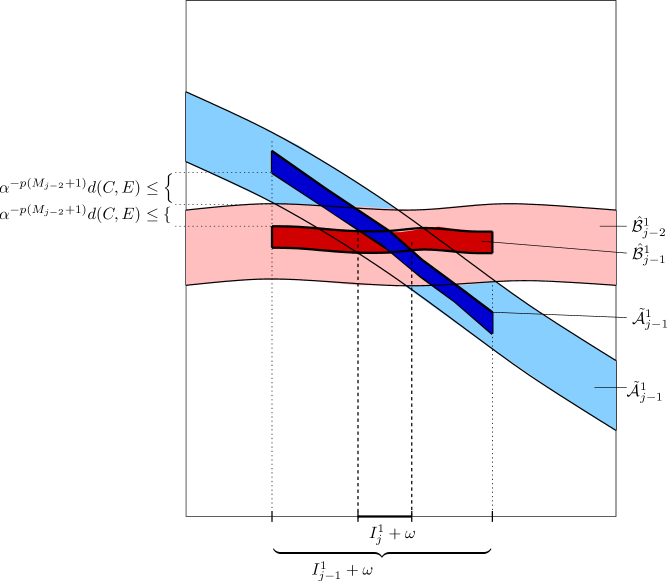
Figure 6.2: Proof of Claim 6.2: The ‘downwards’ crossing between $\tilde{\mathcal{A}}_{j}^{1}$ and $\hat{\mathcal{B}}_{j}^{1}$.

We now turn to the proof of Lemma 5.4. For $\tau\in\Gamma$, by Lemma 5.1 and Proposition 4.6, we have that $(\mathcal{X})_{n-1},(\mathcal{Y}^{\prime\prime})_{n}$ are satisfied and $|I_{n}^{1}(\tau)|,|I_{n}^{2}(\tau)|\leq\varepsilon_{n}$.

Due to the definition of $J$, we have

(6.9) $$J\subseteq B_{9\varepsilon_{n}}(I_{n}^{1}+k\omega)\cap B_{9\varepsilon_{n}}(I_{n}^{2}),$$

which implies $J+(M_{n}-k+1)\omega\subseteq B_{9\varepsilon_{n}}(I_{n}^{1}+(M_{n}+1)\omega)$. Since $9\varepsilon_{n}\leq\varepsilon_{n-1}$, $(\mathcal{Y}^{\prime\prime})_{n}$ yields

$$(J+(M_{n}-k+1)\omega)\cap\mathcal{V}_{n-1}^{+}=\emptyset.$$

Condition $(\mathcal{X})_{n-1}$ and (6.4), (6.9) also imply that

$$(J+\omega)\cap\mathcal{W}^{-}_{n-1}=\emptyset.$$

Therefore, by (6.2), Lemma 4.4 implies that $\mathcal{B}^{\prime\prime}\subseteq(J+\omega)\times E$. Moreover, since $(J+\omega)\subseteq I_{n-1}^{2}+\omega$ by (6.4) and (6.9), and

$$\big{(}J+(M_{n}-k+1)\omega-l\omega\big{)}\cap(\mathcal{I}_{n}+\omega)=\emptyset\ \ \textrm{for}\ \ 0\leq l\leq M_{n}-k-1,$$

by (6.2), we can apply Lemma 4.9 with $N=M_{n}-k$ and $\phi(\theta)=e^{\pm}$ to obtain that for any $\theta\in J+\omega$,

$$|\mathcal{B}_{\theta}^{\prime\prime}|\ \leq\ |E|\alpha^{-\frac{M_{n}-k}{p}},\ \textrm{and}\ \$$

$$|\partial_{\theta}\varphi_{\mathcal{B}^{\prime\prime}}^{\pm}(\theta)|\ \leq\ \sum_{l=1}^{M_{n}-k}\alpha^{-\frac{l}{p}}S\leq\frac{1}{\alpha^{1/p}-1}S.$$

∎

6.4 Proof of Lemma 5.5

For $\tau\in\Gamma$, by Lemma 5.1, we have that $(\mathcal{X})_{n-1}$, $(\mathcal{Y}^{\prime\prime})_{n}$ hold and $d(I_{n}^{1}+k\omega,I_{n}^{2})\leq 4\varepsilon_{n}$. Let $\mathcal{A}^{\prime\prime\prime}=f^{M_{n}-k}(\mathcal{A}^{\prime})$. Then for $\theta\in J+\omega$, we have

$$\varphi_{\mathcal{A}^{\prime\prime}}^{\pm}(\theta)=f_{\theta-k\omega}^{k}(\varphi_{\mathcal{A}^{\prime\prime\prime}}^{\pm}(\theta-k\omega)).$$

We first derive the estimates for the shape of $\mathcal{A}^{\prime\prime\prime}$. Since $(J-k\omega)\subseteq I_{n-1}^{1}$ by (6.4) and (6.9), $\big{(}J-(M_{n}-1)\omega+l\omega\big{)}\cap\mathcal{I}_{n}=\emptyset$ for $0\leq l\leq M_{n}-k-2$ by (6.2), and $(J-(M_{n}-1)\omega)\cap\mathcal{Y}_{n-1}=\emptyset$ by $(\mathcal{Y}^{\prime\prime})_{n}$ and (6.9). Therefore, we can apply Lemma 4.8 to obtain that

(6.10) $$|\mathcal{A}_{\theta}^{\prime\prime\prime}|\leq\alpha^{-\frac{M_{n}-k}{p}}|C|,$$

(6.11) $$-S-\frac{S}{\alpha^{1/p}-1}\leq\partial_{\theta}\varphi_{\mathcal{A}^{\prime\prime\prime}}^{\pm}(\theta)\leq-s+\frac{S}{\alpha^{1/p}-1}$$

for all $\theta\in J-(k-1)\omega$.

Now in order to obtain the required estimates on $\mathcal{A}^{\prime\prime}$, we let $\phi^{\iota}(\theta-k\omega)=\varphi_{\mathcal{A}^{\prime\prime\prime}}^{\pm}(\theta-k\omega)$ $(\iota=1,2)$ for $\theta\in J+\omega$. Then Remark 4.10 yields

$$|\mathcal{A}_{\theta}^{\prime\prime}|\ \leq\ \alpha^{pk}\alpha^{-\frac{M_{n}-k}{p}}|C|,$$

$$|\partial_{\theta}\varphi_{\mathcal{A}^{\prime\prime}}^{\pm}(\theta)|\ \leq\ \frac{2\alpha^{p(k+1)}S}{\alpha^{p}-1}.$$

∎

6.5 Proof of Lemma 5.6

Since $J-(k-M_{n-1}-1)\omega\subseteq I_{n-1}^{1}+(M_{n-1}+1)\omega$ and $J-(M_{n-1}-1)\omega\subseteq I_{n-1}^{2}-(M_{n-1}-1)\omega$ by (6.4) and (6.9), conditions $(\mathcal{X})_{n-1}$ and $(\mathcal{Y}^{\prime\prime})_{n-1}$ imply that

(6.12) $$(J-(k-M_{n-1}-1)\omega)\cap\mathcal{V}_{n-1}^{-}=\emptyset,$$

and

(6.13) $$(J-(M_{n-1}-1)\omega)\cap\mathcal{W}^{+}_{n-1}=\emptyset.$$

Then by (6.2) and Lemma 4.3, we have $f^{k-2M_{n-1}}(\mathcal{D})\subseteq(J-(M_{n-1}-1)\omega)\times C$. Combined with (6.3), this yields

$$\mathcal{D}^{\prime}\subseteq f^{M_{n-1}}(\mathcal{A}_{n-1}^{2})\subseteq(I_{n-1}^{2}+\omega)\times E.$$

Because $(J-(k-M_{n-1}-1)\omega+l\omega)\cap\mathcal{I}_{n}=\emptyset$ for $0\leq l\leq k-M_{n-1}-2$ by (6.2), and $J\subseteq I_{n-1}^{2}$ by (6.4) and (6.9), we can apply Lemma 4.8 with $I=J-(k-M_{n-1}-1)\omega,\ N=k-M_{n-1}-1,\ \phi^{\iota}=c^{\pm}$ $(\iota=1,2)$, together with (4.34), to obtain that for all $\theta\in J+\omega$

$$|C|\cdot\alpha^{-p(k-M_{n-1})}\ \leq\ |\mathcal{D}_{\theta}^{\prime}|\ \leq\ |C|\cdot\alpha^{-\frac{k-M_{n-1}}{p}},$$

$$s-\frac{S}{\alpha^{1/p}-1}\ \leq\ \partial_{\theta}\varphi_{\mathcal{D}^{\prime}}^{\pm}(\theta)\ \leq\ S+\frac{S}{\alpha^{1/p}-1}.$$

∎

6.6 Proof of Lemma 5.7

As before, we fix $\tau\in\Gamma$ such that assertions $(i)$-$(iii)$ of Lemma 5.1 hold.

Since $\mathcal{A}^{\prime\prime}\cap\mathcal{D}^{\prime}=f^{k}\big{(}f^{M_{n}-k}(\mathcal{A}^{\prime})\cap f^{-M_{n-1}}(\mathcal{D})\big{)}$, we have $\pi_{1}\left(\mathcal{A}^{\prime\prime}\cap\mathcal{D}^{\prime}\right)=\pi_{1}\big{(}f^{M_{n}-k}(\mathcal{A}^{\prime})\cap f^{-M_{n-1}}(\mathcal{D})\big{)}+k\omega$. In the following, we will focus on $f^{M_{n}-k}(\mathcal{A}^{\prime})\cap f^{-M_{n-1}}(\mathcal{D})$. We let $\mathcal{A}^{\prime\prime\prime}=f^{M_{n}-k}(\mathcal{A}^{\prime})$ as before and set

$$\mathcal{D}_{\iota}=\left(J-(k-M_{n-1}-1)\omega\right)\times X_{\iota},\ \ \ \hat{\mathcal{D}}_{\iota}=f^{-M_{n-1}}(\mathcal{D}_{\iota}),\ \ \iota=1,2,3,c,$$

where $X_{1}=[c^{+},e^{-}],X_{2}=E,X_{3}=[e^{+},c^{-}]$ and $X_{c}=[c^{+},c^{-}]$. Note that $\varphi_{\hat{\mathcal{D}}_{c}}^{\pm}(\theta)=\varphi_{f^{-M_{n-1}}(\mathcal{D})}^{\mp}(\theta)$ for $\theta\in J-(k-1)\omega$.

We will first prove that $\mathcal{A}^{\prime\prime\prime}$ crosses $\hat{\mathcal{D}}_{c}$ exactly once and this crossing is downwards (see Figure 6.3).

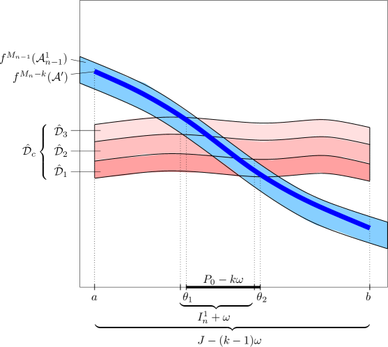
Figure 6.3: Proof of Lemma 5.7: The definition of $P_{0}$.

The reason is as follows. Since $J-(k+M_{n-1}-1)\omega\subseteq I_{n-1}^{1}-(M_{n-1}-1)\omega$ by (6.4) and (6.9), and $(I_{n-1}^{1}-(M_{n-1}-1)\omega)\cap\mathcal{W}^{-}_{n-1}=\emptyset$ by conditions $(\mathcal{X})_{n-1},\ (\mathcal{Y}^{\prime\prime})_{n-1}$, we have $(J-(k+M_{n-1}-1)\omega)\cap\mathcal{W}^{-}_{n-1}=\emptyset$. Together with (6.2) and the fact that $(J-(M_{n}-1)\omega)\cap\mathcal{Y}_{n-1}=\emptyset$ by (6.9) and $(\mathcal{Y}^{\prime\prime})_{n}$, Lemma 4.3 implies $f^{M_{n}-k-M_{n-1}}(\mathcal{A}^{\prime})\subseteq\mathcal{A}_{n-1}^{1}$ and hence

$$\mathcal{A}^{\prime\prime\prime}\ \subseteq\ f^{M_{n-1}}(\mathcal{A}_{n-1}^{1}).$$

Recall that $I_{n}^{\iota}=(a_{n}^{\iota},b_{n}^{\iota}),\iota=1,2$. By the definition of $I_{n}^{1}$, we have

(6.14) $$\varphi_{\mathcal{A}^{\prime\prime\prime}}^{-}(a_{n}^{1}+\omega)\geq\varphi_{f^{M_{n-1}}(\mathcal{A}_{n-1}^{1})}^{-}(a_{n}^{1}+\omega)\ =\ \varphi_{\hat{\mathcal{D}}_{3}}^{-}(a_{n}^{1}+\omega)\ .$$

Since $J-(k-M_{n-1}-1)\omega\subseteq I_{n-1}^{1}+(M_{n-1}+1)\omega$ and $J-(k-1)\omega\subseteq I_{n-1}^{1}+\omega$ by (6.4) and (6.9) and $(J-(k-M_{n-1}-1)\omega-l\omega)\cap(\mathcal{I}_{n}+\omega)=\emptyset$ for $l=0,1,\ldots,M_{n-1}-1$ by (6.2), we can apply Lemma 4.9, together with (4.34) to obtain that

$$|X_{\iota}|\cdot\alpha^{-pM_{n-1}}\ \leq\ |\hat{\mathcal{D}}_{\iota,\theta}|\ \leq\ |X_{\iota}|\cdot\alpha^{-\frac{M_{n-1}}{p}},\ \ \ |\partial_{\theta}\varphi_{\hat{\mathcal{D}}_{\iota}}^{\pm}(\theta)|\ \leq\ \frac{S}{\alpha^{1/p}-1},$$

for all $\theta\in J-(k-1)\omega$ and $\iota=1,2,3,c$.

Writing $J-(k-1)\omega=:[a,b]$ and using (6.10) and (6.11), we obtain

$$\varphi_{\mathcal{A}^{\prime\prime\prime}}^{-}(a)-\varphi_{\hat{\mathcal{D}}_{3}}^{-}(a)\ \stackrel{{\scriptstyle\eqref{e.graph_equality}}}{{\geq}}\ \varphi_{\mathcal{A}^{\prime\prime\prime}}^{-}(a)-\varphi_{\mathcal{A}^{\prime\prime\prime}}^{-}(a_{n}^{1}+\omega)+\varphi_{\hat{\mathcal{D}}_{3}}^{-}(a_{n}^{1}+\omega)-\varphi_{\hat{\mathcal{D}}_{3}}^{-}(a)$$

$$\geq (s-\frac{S}{\alpha^{1/p}-1})\cdot(a_{n}^{1}+\omega-a)-\frac{S}{\alpha^{1/p}-1}\cdot(a_{n}^{1}+\omega-a)\hskip 40.00006pt$$

$$\stackrel{{\scriptstyle(\alpha)}}{{\geq}} \frac{s}{2}\cdot 4\varepsilon_{n}\geq 4\alpha^{-\frac{M_{n-1}}{p}}>\sup_{\theta\in J-(k-1)\omega}|\hat{\mathcal{D}}_{3,\theta}|,$$

which means

$$\varphi_{\mathcal{A}^{\prime\prime\prime}}^{-}(a)>\varphi_{\hat{\mathcal{D}}_{3}}^{+}(a)=\varphi_{\hat{\mathcal{D}}_{c}}^{+}(a).$$

Similarly, we obtain

$$\varphi_{\mathcal{A}^{\prime\prime\prime}}^{+}(b)<\varphi_{\hat{\mathcal{D}}_{1}}^{-}(b)=\varphi_{\hat{\mathcal{D}}_{c}}^{-}(b).$$

Thus, together with the fact that $\inf_{\theta\in J-(k-1)\omega}|\partial_{\theta}\varphi_{\mathcal{A}^{\prime\prime\prime}}^{\pm}(\theta)|>\sup_{\theta\in J-(k-1)\omega}|\partial_{\theta}\varphi_{\hat{\mathcal{D}}_{c}}^{\pm}(\theta)|,$ we have that $\mathcal{A}^{\prime\prime\prime}$ ‘downwards’ crosses $\hat{\mathcal{D}}_{c}$ exactly one time, which means that in the image the boundary curves of $\mathcal{A}^{\prime\prime}$ intersect those of $\mathcal{D}^{\prime}$ exactly once. Equivalently,

$$\left.\begin{array}[]{ll}&\exists!\ \theta_{1}\in J-(k-1)\omega\ \ \textrm{with}\ \varphi_{\mathcal{A}^{\prime\prime\prime}}^{+}(\theta_{1})=\varphi_{\hat{\mathcal{D}}_{c}}^{+}(\theta_{1})\ \textrm{and}\\ &\exists!\ \theta_{2}\in J-(k-1)\omega\ \ \textrm{with}\ \varphi_{\mathcal{A}^{\prime\prime\prime}}^{-}(\theta_{2})=\varphi_{\hat{\mathcal{D}}_{c}}^{-}(\theta_{2}).\end{array}\right.$$

Then we have

$$\varphi_{\mathcal{A}^{\prime\prime\prime}}^{-}(\theta_{1})-\varphi_{\hat{\mathcal{D}}_{c}}^{-}(\theta_{1}) = (\varphi_{\hat{\mathcal{D}}_{c}}^{+}(\theta_{1})-\varphi_{\hat{\mathcal{D}}_{c}}^{-}(\theta_{1}))-(\varphi_{\mathcal{A}^{\prime\prime\prime}}^{+}(\theta_{1})-\varphi_{\mathcal{A}^{\prime\prime\prime}}^{-}(\theta_{1}))$$

$$\geq \inf_{\theta\in J-(k-1)\omega}|\hat{\mathcal{D}}_{c,\theta}|-\sup_{\theta\in J-(k-1)\omega}|\mathcal{A}_{\theta}^{\prime\prime\prime}|,$$

$$\varphi_{\mathcal{A}^{\prime\prime\prime}}^{-}(\theta_{1})-\varphi_{\hat{\mathcal{D}}_{c}}^{-}(\theta_{1})\ \leq\ \sup_{\theta\in J-(k-1)\omega}|\hat{\mathcal{D}}_{c,\theta}|$$

$$s/2\ <\ \partial_{\theta}(\varphi_{\hat{\mathcal{D}}_{c}}^{-}(\theta)-\varphi_{\mathcal{A}^{\prime\prime\prime}}^{-}(\theta))\ <\ 2S.$$

Therefore, for $\alpha$ large, we obtain that

(6.15) $$\frac{(1-|C|)}{4S}\cdot\alpha^{-pM_{n-1}}\ <\ \theta_{2}-\theta_{1}\ <\ \frac{4(1-|C|)}{s}\cdot\alpha^{-M_{n-1}/p}.$$

Moreover, if we let $\tilde{\mathcal{A}}_{n-1}^{1}=f^{M_{n-1}}(\mathcal{A}_{n-1}^{1})$, then by the definition of $I_{n}^{1}$, we have $\varphi_{\tilde{\mathcal{A}}_{n-1}^{1}}^{+}(b_{n}^{1}+\omega)=\varphi_{\hat{\mathcal{D}}_{2}}^{-}(b_{n}^{1}+\omega)$. Because $\partial_{\theta}(\varphi_{\tilde{\mathcal{A}}_{n-1}^{1}}^{+}-\varphi_{\hat{\mathcal{D}}_{2}}^{-})<-s/2<0$, and

$$\varphi_{\tilde{\mathcal{A}}_{n-1}^{1}}^{+}(\theta_{1})-\varphi_{\hat{\mathcal{D}}_{2}}^{-}(\theta_{1})>\varphi_{\mathcal{A}^{\prime\prime\prime}}^{+}(\theta_{1})-\varphi_{\hat{\mathcal{D}}_{2}}^{-}(\theta_{1})>\varphi_{\mathcal{A}^{\prime\prime\prime}}^{+}(\theta_{1})-\varphi_{\hat{\mathcal{D}}_{3}}^{+}(\theta_{1})=0,$$

we get $\theta_{1}<b_{n}^{1}+\omega$. Similarly, we obtain $\theta_{2}>a_{n}^{1}+\omega$, which implies that $(\theta_{1},\theta_{2})\cap(I_{n}^{1}+\omega)\neq\emptyset$.

If we now let $P_{0}=(\theta_{1}+k\omega,\theta_{2}+k\omega)$, then by the selection of $\theta_{1}$ and $\theta_{2}$, we have

$$\pi_{1}(\mathcal{A}^{\prime\prime}\cap\mathcal{D}^{\prime})\cap P_{0}=\emptyset,$$

with $\frac{(1-|C|)}{4S}\cdot\alpha^{-pM_{n-1}}<|P_{0}|<\frac{4(1-|C|)}{s}\cdot\alpha^{-M_{n-1}/p}$ and $P_{0}\cap(I_{n}^{1}+(k+1)\omega)\neq\emptyset$. ∎

6.7 Proof of Lemma 5.8

For $\theta\in I_{0}^{2}+\omega$, we let

$$\zeta(\theta)\ =\ c^{-}+\min\left\{\varphi_{f(I_{0}^{2}\times(\mathbb{T}^{1}\setminus E))}^{-}(\theta)-\varphi_{f(I_{0}^{2}\times(\mathbb{T}^{1}\setminus E))}^{-}(a_{0}^{2}+\omega),c^{+}-c^{-}\right\}\ ,$$

and choose $\xi$ to be a small $\mathcal{C}^{1}$-perturbation of $\zeta$ which satisfies $\xi(\theta)\in C$ and $|\partial_{\theta}\xi(\theta)|\leq S$ by (${\cal A}5$) (see Figure 6.4).

Figure 6.4: Proof of Lemma 5.8: Construction of the curves $\zeta$ and $\xi$.

Then, we let $\Xi=\{(\theta,\xi(\theta))\ |\ \theta\in J+\omega\}\subseteq(J+\omega)\times C$. Since the graph of $\zeta$ is disjoint from $f(J\times(\mathbb{T}^{1}\setminus E))$, we can choose $\xi$ sufficiently close to $\zeta$ such that this still holds, that is,

(6.16) $$\Xi\cap f(J\times(\mathbb{T}^{1}\setminus E))\ =\ \emptyset\ .$$

In order to verify that $\pi_{1}(\Xi\cap\mathcal{A}^{\prime\prime})$ is an iterval, we consider the preimage $f^{-k}(\Xi)$ and show that this curve intersects $f^{-k}(\mathcal{A}^{\prime\prime})$ in a transversal way (see Figure 6.5).

Let $\Upsilon=f^{-1}(\Xi)=:\{(\theta,v(\theta))\ |\ \theta\in J\}$. Then, by (6.16) above, $\Upsilon\subseteq J\times E$. Moreover, as $v(\theta)\in E$ for all $\theta\in J$, we have

$$|\partial_{\theta}v(\theta)| = |(\partial_{x}f_{\theta+\omega}^{-1})(\xi(\theta+\omega))\cdot\partial_{\theta}\xi(\theta+\omega)+(\partial_{\theta}f_{\theta+\omega}^{-1})(\xi(\theta+\omega))|$$

$$= \left|\frac{1}{(\partial_{x}f_{\theta})(v(\theta))}\cdot\partial_{\theta}\xi(\theta+\omega)-\frac{(\partial_{\theta}f_{\theta})(v(\theta))}{(\partial_{x}f_{\theta})(v(\theta))}\right|$$

$$\leq \alpha^{-2/p}\cdot S+\alpha^{-2/p}\cdot S\stackrel{{\scriptstyle(\alpha)}}{{\leq}}S.$$

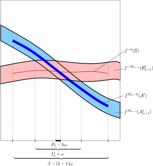
Figure 6.5: Transversal intersection between $f^{-k}(\Xi)$ and $f^{-k}(\mathcal{A}^{\prime\prime})=f^{M_{n}-k}(\mathcal{A}^{\prime})$.

Let $\mathcal{A}^{\prime\prime\prime}:=f^{M_{n}-k}(\mathcal{A}^{\prime})$ as before and $\Psi(\theta):=f_{\theta+(k-1)\omega}^{-(k-1)}(\upsilon(\theta+(k-1)\omega))$, where $\theta\in J-(k-1)\omega$. Since $J\subseteq I_{n-1}^{2}\subseteq I_{n-2}^{2}\subseteq\ldots\subseteq I_{0}^{2}$ by (6.4) and (6.9), condition $(\mathcal{X})_{n-1}$ yields

(6.17) $$J\cap\mathcal{V}_{n-1}^{+}=\emptyset.$$

Further, as $J-(k-M_{n-1}-1)\omega\subseteq I_{n-1}^{1}+(M_{n-1}+1)\omega$ by (6.4), (6.9), conditions $(\mathcal{X})_{n-1}$ and $(\mathcal{Y}^{\prime\prime})_{n-1}$ imply $(J-(k-M_{n-1}-1)\omega)\cap\mathcal{W}^{-}_{n-1}=\emptyset$. Together with (6.2), Lemma 4.4 yields

$$f^{-(k-M_{n-1}-1)}(\Upsilon)\ \subseteq\ \big{(}J-(k-M_{n-1}-1)\omega\big{)}\times E\ \subseteq\mathcal{B}^{1}_{n-1}\ .$$

Thus, we obtain

(6.18) $$f^{-(k-1)}(\Upsilon)\subseteq f^{-M_{n-1}}(\mathcal{B}_{n-1}^{1})\subseteq(I_{n-1}^{1}+\omega)\times E.$$

Moreover, Lemma 6.1 yields that $(J-l\omega)\cap(\mathcal{I}_{n}+\omega)=\emptyset$ for $l=0,\ldots,k-2$. Therefore (6.17) and the fact that $J-(k-1)\omega\subseteq I_{n-1}^{1}+\omega$ by (6.4) and (6.9) allow to apply Lemma 4.9 in order to obtain

$$\sup_{\theta\in J-(k-1)\omega}|\partial_{\theta}\Psi|\ \leq\ \frac{S}{\alpha^{1/p}-1}.$$

Then by (6.11), we get $\inf_{\theta}|\partial_{\theta}\varphi_{\mathcal{A}^{\prime\prime\prime}}^{\pm}(\theta)|\stackrel{{\scriptstyle(\alpha)}}{{>}}\sup_{\theta}|\partial_{\theta}\Psi|$. Thus, by the same argument as in Section 6.6, $\mathcal{A}^{\prime\prime\prime}$ is above $f^{-(k-1)}(\Upsilon)$ on the left end of $J-(k-1)\omega$ and below on the right end by (6.18) (see Figure 6.4). Therefore the boundary curves of $\mathcal{A}^{\prime\prime\prime}$ intersect $f^{-(k-1)}(\Upsilon)$ exactly once, which means $\pi_{1}\left(\mathcal{A}^{\prime\prime\prime}\cap f^{-(k-1)}(\Upsilon)\right)$ is an interval. Hence $P_{1}=\pi_{1}(\mathcal{A}^{\prime\prime}\cap\Xi)=\pi_{1}\left(\mathcal{A}^{\prime\prime\prime}\cap f^{-(k-1)}(\Upsilon)\right)+k\omega$ is an interval. ∎

6.8 Proof of Lemma 5.11

We will first prove that $(\mathcal{X})_{n}$ actually holds for $\tau=\tau^{-},\tau^{+}$. By Lemma 5.1 and Proposition 4.6, we have $|I_{n}^{\iota}(\tau^{\pm})|\leq\varepsilon_{n},\ \iota=1,2$, and $d(I_{n}^{1}(\tau^{\pm})+k\omega,I_{n}^{2}(\tau^{\pm}))=4\varepsilon_{n}$. If $d_{H}$ denotes the Hausdorff distance, then $d_{H}(I_{n}^{1}(\tau^{\pm})+k\omega,I_{n}^{2}(\tau^{\pm}))\leq 5\varepsilon_{n}$. Include $\tau^{\pm}$ throughout the proof. The Diophantine condition $\omega\in\mathcal{D}(\gamma,\nu)$ implies $d(I_{n}^{\iota},I_{n}^{\iota}+j\omega)>8\varepsilon_{n}$ for $\iota=1,2,\ j\in[1,(2K_{n}+1)M_{n}]$ by (4.3) and (4.4), provided $\alpha$ is large. Then, given $l\in[1,2K_{n}M_{n}]\setminus\{k\}$, we have

$$d(I_{n}^{2},I_{n}^{1}+l\omega)\geq d(I_{n}^{1}+l\omega,I_{n}^{1}+k\omega)-d_{H}(I_{n}^{1}+k\omega,I_{n}^{2})\ >\ 8\varepsilon_{n}-5\varepsilon_{n}=3\varepsilon_{n},\$$

and similarly

$$d(I_{n}^{1},I_{n}^{2}+l\omega)\ \geq\ 3\varepsilon_{n}\ .$$

Moreover, by the choice of $\tau^{-},\tau^{+}$ in Section 6.1, we have $d(I_{n}^{2},I_{n}^{1}+k\omega)>3\varepsilon_{n}$. Thus, $(\mathcal{X})_{n}$ is satisfied.

Hence, Proposition 4.6 implies that the two components of $\mathcal{I}_{n+1}$ are non-empty, which means $f^{M_{n}}(\mathcal{A}_{n}^{2})\cap f^{-M_{n}}(\mathcal{B}_{n}^{2})\neq\emptyset$. Then Lemma 5.3 implies that $\mathcal{B}^{\prime\prime}\cap f^{M_{n}}(\mathcal{A}_{n}^{2})\neq\emptyset$. Moreover, Lemma 5.7 implies that $P_{0}\cap(I_{n}^{1}+(k+1)\omega)\neq\emptyset$. Since $|P_{0}|\leq 2\varepsilon_{n}$ (using the estimate from Lemma 5.7 and (4.4)), and $d(I_{n}^{1}+k\omega,I_{n}^{2})=4\varepsilon_{n}$, we get $P_{0}\cap(I_{n}^{2}+\omega)=\emptyset$. When $\tau=\tau^{-}$, then since $I_{n}^{2}$ is to the right of $I_{n}^{1}+k\omega$, we have $f^{M_{n}}(\mathcal{A}_{n}^{2})\subseteq\mathcal{R}$, which means $\mathcal{B}^{\prime\prime}$ intersects $\mathcal{R}$. Conversely, when $\tau=\tau^{+}$ we have $f^{M_{n}}(\mathcal{A}_{n}^{2})\subseteq\mathcal{L}$ since $I_{n}^{2}$ is to the left of $I_{n}^{1}+k\omega$ and thus $\mathcal{B}^{\prime\prime}$ intersects $\mathcal{L}$.∎

References

- [1] A. Katok and B. Hasselblatt. Introduction to the Modern Theory of Dynamical Systems. Cambridge University Press, 1997.
- [2] EJ Ding. Analytic treatment of periodic orbit systematics for a nonlinear driven oscillator. Physical Review A, 34(4):3547, 1986.
- [3] V.I. Arnold. Cardiac arrythmias and circle mappings. Chaos, 1(1):20–24, 1991. These results were already contained in the authors 1959 PhD thesis at the Moscow University, but were omitted in the published version of that work (Am. Math. Soc. Transl. 46(2):213–284, 1965).
- [4] D.H. Perkel, J.H. Schulman, T.H. Bullock, G.P. Moore, and J.P. Segundo. Pacemaker neurons: Effects of regularly spaced synaptic input. Science, 145:61–63, 1964.
- [5] S. Coombes and P.C. Bressloff. Mode locking and arnold tongues in integrate-and-fire neural oscillators. Phys. Rev. E, 60(2):2086, 1999.
- [6] R. Johnson and J. Moser. The rotation numer for almost periodic potentials. Commun. Math. Phys., 4:403–438, 1982.
- [7] M. Herman. Une méthode pour minorer les exposants de Lyapunov et quelques exemples montrant le caractère local d’un théorème d’Arnold et de Moser sur le tore de dimension 2. Comment. Math. Helv., 58:453–502, 1983.
- [8] A. Haro and J. Puig. Strange non-chaotic attractors in Harper maps. Chaos, 16, 2006.
- [9] J. B\a’ellissard and B. Simon. Cantor spectrum for the almost Mathieu equation. J. Funct. Anal., 48(3):408–419, 1982.
- [10] J. Puig. Cantor spectrum for the almost Mathieu operator. Commun. Math. Phys., 244(2):297–309, 2004.
- [11] A. Avila and S. Jitomirskaya. The Ten Martini Problem. Ann. Math. (2), 170(1):303–342, 2009.
- [12] M. Benedicks and L. Carleson. The dynamics of the Hénon map. Ann. Math. (2), 133(1):73–169, 1991.
- [13] L.-S. Young. Lyapunov exponents for some quasi-periodic cocycles. Ergodic Theory Dyn. Syst., 17:483–504, 1997.
- [14] K. Bjerklöv. Positive Lyapunov exponent and minimality for a class of one-dimensional quasi-periodic Schrödinger equations. Ergodic Theory Dyn. Syst., 25:1015–1045, 2005.
- [15] K. Bjerklöv. Dynamics of the quasiperiodic Schrödinger cocycle at the lowest energy in the spectrum. Commun. Math. Phys., 272:397–442, 2005.
- [16] T. Jäger. Strange non-chaotic attractors in quasiperiodically forced circle maps. Comm. Math. Phys., 289(1):253–289, 2009.
- [17] G. Fuhrmann. Non-smooth saddle-node bifurcations of forced monotone interval maps i: Existence of an sna. Preprint 2013, arXiv:1307.0347.
- [18] K. Bjerklöv and T. Jäger. Rotation numbers for quasiperiodically forced circle maps – Mode-locking vs strict monotonicity. J. Am. Math. Soc., 22(2):353–362, 2009.
- [19] C. Grebogi, E. Ott, S. Pelikan, and J.A. Yorke. Strange attractors that are not chaotic. Physica D, 13:261–268, 1984.
- [20] G. Keller. A note on strange nonchaotic attractors. Fundam. Math., 151(2):139–148, 1996.
- [21] T. Jäger. Strange non-chaotic attractors in quasiperiodically forced circle maps: Diophantine forcing. To appear in Ergodic Theory Dyn. Syst., published online at http://dx.doi.org/10.1017/S0143385712000375, 2013.
- [22] U. Feudel, J. Kurths, and A. Pikovsky. Strange nonchaotic attractor in a quasiperiodically forced circle map. Physica D, 88:176–186, 1995.
- [23] P. Glendinning, U. Feudel, A. Pikovsky, and J. Stark. The structure of mode-locked regions in quasi-periodically forced circle maps. Physica D, 140:227–243, 2000.
- [24] K. Bjerklöv. The dynamics of a class of quasi-periodic schrödinger cocycles. Ann. H. Poincaré, pages 1–71, 2014. published online 04 May 2014, DOI 10.1007/s00023-014-0330-8.
- [25] Y. Wang and Z. Zhang. Uniform positivity and continuity of lyapunov exponents for a class of quasiperiodic schrödinger cocycles. Preprint 2013, arXiv:1311.4282.
- [26] Y. Wang and Z. Zhang. Cantor spectrum for a class of quasiperiodic Schrödinger operators. Preprint 2014, arXiv:1410.0101.
- [27] T. Jäger. The creation of strange non-chaotic attractors in non-smooth saddle-node bifurcations. Mem. Am. Math. Soc., 945:1–106, 2009.
- [28] K. Bjerklöv. Positive Lyapunov exponent and minimality for the continuous 1-d quasi-periodic Schrödinger equation with two basic frequencies. Ann. Henri Poincaré, 8(4):687–730, 2007.
- [29] J. Stark and R. Sturman. Semi-uniform ergodic theorems and applications to forced systems. Nonlinearity, 13(1):113–143, 2000.