The chemistry of planetary nebulae in the outer regions of M31

Abstract

We present spectroscopy of nine planetary nebulae (PNe) in the outskirts of M31, all but one obtained with the 10.4 m GTC telescope. These sources extend our previous study of the oxygen abundance gradient of M31 to galactocentric radii as large as 100 kpc. None of the targets are bona fide members of a classical, metal-poor and ancient halo. Two of the outermost PNe have solar oxygen abundances, as well as radial velocities consistent with the kinematics of the extended disk of M31. The other PNe have a slightly lower oxygen content ([O/H]$\sim$$-0.4$) and in some cases large deviations from the disk kinematics. These PNe support the current view that the external regions of M31 are the result of a complex interaction and merger process, with evidence for a widespread population of solar–metallicity stars produced in a starburst that occurred $\sim$2 Gyr ago.

1 Introduction

Planetary nebulae (PNe) are valuable tracers of stellar populations in all types of galaxies. They are widely used as distance indicators, via the invariant bright cutoff of the PN luminosity function (PNLF; e.g. Ciardullo et al., 2002), and as tracers of the luminosity (Buzzoni, Arnaboldi, & Corradi, 2006), dynamics (e.g. Merrett et al., 2006) and chemistry (e.g. Kwitter et al. 2012; Balick et al. 2013, hereafter papers I and II, respectively) of their stellar progenitors.

Recently, PNe have been used to determine the metallicity gradient in the disk of the nearby spiral galaxies M33 (Magrini, Stanghellini & Villaver, 2009) and M31 (papers I and II). These gradients provide direct constraints to models of disk formation and evolution. In particular, measurements in the outer regions of the disks have the power to test novel ideas such as the importance of external disturbances to produce extended young stellar disks (Werk et al., 2011). In the case of M31, it has been proposed that a tidal encounter with M33 that occurred about 3 Gyr ago would have produced a vast extended disk with homogeneous metallicity (Bernard et al., 2012, 2015). Such an extended disk has been reported before (Ibata et al., 2005), and PNe provide the opportunity to test its predicted chemical content. In earlier papers, we have studied PNe out to deprojected galactocentric distances of 60 kpc, finding nearly solar O/H abundances and a flat O/H gradient in these regions. In this work, we extend our study by obtaining high-quality spectra of another nine PNe at larger radii in the outskirts of M31.

Table 1: Basic properties of the target PNe

Name	R.A. pippppDec		m($5007$)	$\xi$	$\eta$	$d_{app}$	$d_{app}$	$d_{disk}$	V⊙,sys	Vdiff
	[J2000]	[J2000]	[mag]	[deg]	[deg]	[deg]	[kpc]	[kpc]	[km s-1]	[km s-1]
M2507	00 48 27.2	+39 55 34.3	21.23	1.10	-1.33	1.73	23.2	106.3	-147	180
M2538	00 36 28.8	+39 35 26.4	20.25	-1.21	-1.67	2.06	27.7	28.0	-426	110
M2539	00 36 12.6	+39 35 41.9	21.16	-1.26	-1.66	2.08	28.0	28.0	-426	110
M2541	00 35 09.1	+39 28 25.2	21.78	-1.46	-1.78	2.30	31.0	31.3	-456	080
M2543	00 35 50.7	+42 21 04.5	21.61	-1.27	1.09	1.68	22.6	105.8	-272	040
M2549	00 36 27.2	+42 06 21.9	21.35	-1.17	0.85	1.44	19.4	90.9	0-17	290
M2566	00 49 28.3	+40 59 53.9	21.26	1.27	-0.26	1.30	17.4	73.8	-247	010
M2988	00 52 00.0	+43 03 23.5	21.98	1.69	1.81	2.48	33.3	36.2	0-98	020
M31-372	00 46 41.5	+43 59 03.7	22.60	0.71	2.72	2.81	37.8	77.6	0-60	100

Note. — The following parameters for M31 have been assumed throughout the paper: distance 770 kpc (Freedman & Madore, 1990); center at RA(J2000)= 0 42 44.3 and Dec(J2000)=+41 16 09.0 (Merrett et al., 2006); disk inclination $i$=77°.7 (De Vaucouleurs, 1958) and position angle PA=37°.7 (Merrett et al., 2006); heliocentric systemic velocity V_sys=$-309$ kms (Merrett et al., 2006).

Figure 1: The spectra of the target PNe. For the lower S/N spectrum of M2538, regions with high noise have been masked, and the whole spectrum was smoothed with a boxcar of three pixels.

2 Observations

The target PNe are listed in Table 1. All but one were selected from the list of Merrett et al. (2006) to be at large galactocentric distances and sufficiently bright to obtain high quality spectra with a 10m telescope. The putative halo PN M31-372 observed by Jacoby & Ford (1986) was additionally included.

Spectroscopy of eight of these PNe was obtained in different nights in October 2013 in service-queue mode at the 10.4m GTC telescope on the island of La Palma, Spain. The OSIRIS instrument was used in its longslit mode. The combination of grism R1000B and a slit width of $0^{\prime\prime}.8$ provides a spectral dispersion of 0.21 nm per (binned $\times$2) pixel, a resolution of 0.63 nm, and a spectral coverage from 370 to 785 nm. Seeing varied between $0^{\prime\prime}.6$ and $1^{\prime\prime}.1$ (full width at half maximum), and spatial scale along the slit was $0^{\prime\prime}.254$ per binned pixel. Data were generally obtained under photometric weather conditions and grey moon. The slit was oriented along the parallactic angle for all targets and standard stars. Total exposure times per target varied from 120 to 135 min, depending on the brightness of the source, split into three or four sub-exposures. The GTC calibration plan provides, in each observing night, at least one spectrophotometric standard to be used for flux calibration.

Additionally, the PN M2538 was observed with the Dual-Imaging Spectrograph at Apache Point Observatory (New Mexico, USA) in 2011 October. We observed through a 2^′′ slit oriented along the parallactic angle. The B1000 grating provided coverage from 370 to 505 nm at 0.25 nm resolution; the R300 grating covered 520–960 nm at 0.70 nm resolution. Standard bias, flatfield, and emission-lamp exposures were taken and applied to the data. Flux calibration was obtained via observations of the standard star BD+28 4211. We obtained six 20 min integrations of M2538, which were co-added after calibration.

As PNe at the distance of M31 (770 kpc, see Table 1) are spatially unresolved, 1–D spectra were extracted and reduced using twodspec in IRAF.

3 Physics and chemistry of the nebulae

The spectra of the target PNe are displayed in Figure 1. Emission-line fluxes were measured by multi-Gaussian fit using splot. These fluxes are the input for the abundance determinations, carried out with ELSA, our five-level atom code (Johnson et al., 2006). We used the same method as in Papers I and II, in order to produce a homogeneous set of data and abundance estimations. The reader is referred to those articles and to Milingo et al. (2010) for the details of the analysis. The procedure includes corrections of the observed line fluxes for interstellar reddening, using the law of Savage & Mathis (1979), and for the contamination of the hydrogen Balmer lines by coincident recombination lines of He⁺⁺. Dereddened fluxes were used to determine the electron temperature and density $N_{e}$ and $T_{e}$ with the appropriate line diagnostics. Note that $T_{e}$([O III]) was always properly determined, as the auroral line [O III]4363 was accurately detected in all PNe (Figure 1). The same applies for $N_{e}$([S II]), except for M31-372 and M2538 where the [S II]6717,6731 doublet could not be measured and a default $N_{e}$ of 10000 cm^-3 was assumed. In PNe where no direct low-ionization temperature diagnostic has been observed, the determination of the temperature to be used for calculating low-ionization abundances ($T_{e}$([N II])) depends on whether He ii4686 is observed. If it is, we adopt the carefully derived result from Kaler (1986) that applies under this condition, i.e. $T_{e}$([N II])$=$10 300 K. If not, then we derive $T_{e}$([N II]) from $T_{e}$([O III]) according to the prescription from Pagel et al. (1992).

The detected lines allowed the calculation of the abundances of several O, Ar, N, S, and Ne ions. Total abundances were then determined using ionization correction factors (icf) calculated as described in Kwitter & Henry (2001). The observed emission-line measurements, logarithmic reddening parameter c(H$\beta$), $T_{e}$ and $N_{e}$, ionic and total abundances are listed in the tables in Appendix A. They indicate that none of the PNe presented in this paper fulfill the original definition by Peimbert & Torres-Peimbert (1983) for Galactic Type I PNe of having either $\log(N/O)>-0.3$ or He/H$>0.125$. This also applies to most of PNe studied in papers I and II, indicating at most a very moderate N and He enrichment for these bright PNe of M31. The PNe studied in this article also follow the relationships between O/H and other elemental abundances (such as N/O, Ne/H, and Ar/H) discussed in paper I.

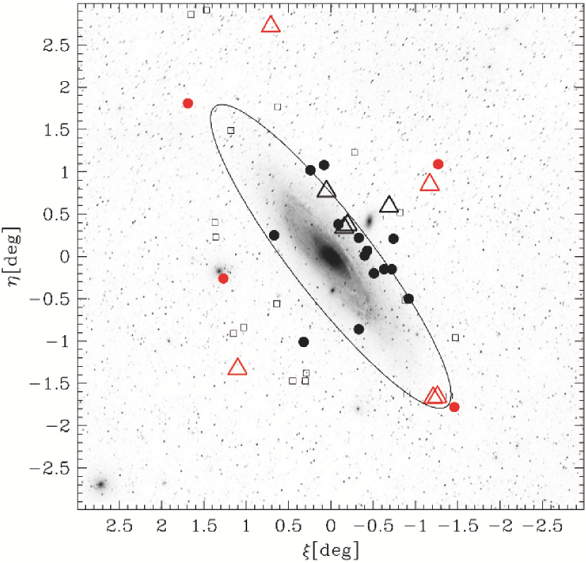
Figure 2: Location of the target PNe, overlaid on the DSS optical image. Circles and triangles indicate PNe with deviations from the model disk kinematics smaller and larger than 100 km s^-1, respectively (see text). Red symbols are the PNe presented in this work, and black symbols those discussed in papers I and II. Squares indicate the HST/ACS fields studied by Bernard et al. (2015). The ellipse indicates the R₂₅ radius of M31.

4 Location of targets within M31

Figure 2 shows the position in the sky of the target PNe, including those discussed in papers I and II. The geometric transformations of Huchra, Brodie & Kent (1991), with the parameters indicated in the Note of Table 1, were adopted to determine the R.A. and Dec offsets $\xi$ and $\eta$ from the center of M31. These offsets, and the total apparent distance $d_{app}$ in the plane of the sky, are also listed in Table 1. The ellipse in the figure marks the R₂₅ radius of M31 ($\sim$30 kpc, see paper II). It corresponds to $\sim$5 scale-lengths of the exponential bright disk of M31 (Walterbos & Kennicutt, 1988), showing that the newly observed PNe are located well outside the familiar bright disk of M31.

These outer regions of M31 are surprisingly complex. A huge halo with a radius $\geq$300 kpc and a smooth star density distribution has been identified (Ibata et al., 2007, 2014). A number of structures, such as streams, loops, and overdensity regions are seen in projection throughout the halo (Lewis et al., 2013; Ibata et al., 2014). They are mostly associated with accretion of satellite dwarf galaxies, as expected in the standard hierarchical halo formation scenario. The most prominent structure is the so-called Giant Stellar Stream (GSS), which is likely the latest, most metal enhanced accretion event associated with the streams. In addition, outside the usual bright disk of M31, a smooth “exodisk” was found to extend out to a galactocentric distance of $\sim$40 kpc, with detections as far as $\sim$70 kpc (Ibata et al., 2005). A set of globular clusters in this zone forms a coherent kinematic system that is similar to an extrapolation of M31’s inner disk (Veljanoski et al., 2014).

As far as metallicity is concerned, there is a significant overlap between the stellar [Fe/H] content of the different structures in the outer regions of M31. Overall, the mean halo metallicity decreases with radius from [Fe/H]$\sim$$-0.7$ at $R\leq$30 kpc to [Fe/H]$\sim$$-1.5$ at $R\sim$150 kpc, but the smooth halo component seems 0.2 dex more metal poor at all radii, and substructures span a wide range in metallicity covering roughly two orders of magnitude (Tanaka et al., 2010; Ibata et al., 2014). The strongest evidence of metal-rich stars in the halo (beyond the bound satellite galaxies) at $\left<[\mbox{Fe/H}]\right>$$\sim$$-0.5$ is found in the GSS (Ibata et al., 2014). As with the extended exodisk, Bernard et al. (2015) find an average value of [Fe/H]$\sim$$-0.3$ for the several disk-like fields considered. Chapman et al. (2006) find several fields in M31’s exodisk in which AGB stars have roughly solar metal abundances. Figure 8 in (Ibata et al., 2014) illustrates the complexity of the metallicity distribution in the outer regions of M31 caused by the overlapping halo (with its ancient and more recent components) and the extended disk.

Adopting the inclination and position angle of M31’s inner disk, the deprojected distances in the plane of the disk for the target PNe, $d_{disk}$, are indicated in Table 1. The radial velocities of PNe provide useful insights into their possible relation to M31’s extended disk. They are adopted from Merrett et al. (2006), except for M31–372 for which a rough estimate could be obtained from our spectra (Table 1). We compared them with the average velocity expected at each position according to the kinematic model of the extended disk presented by Ibata et al. (2005). The most significant differences (V${}_{diff}\geq 100$ km s^-1, see Table 1) are found in PNe M2507, M2538, M2539, M2549, and M31-372, suggesting that they may instead be associated with the halo or some of its substructures.

Bernard et al. (2015) present colour-magnitude diagrams in fourteen HST/ACS fields sampling galactocentric distances similar to the PNe presented in this work. They cover regions of the extended disk of M31, or some of the substructures in the halo, none representing the metal–poor halo component. The positions in the sky of the HST fields are indicated by squares in Figure 2. While some of these fields are not far from our PNe, no noteworthy association can be identified, except for the case of M2538, M2539, and M2541 which seem related to the so-called Warp and G1 Clump, which are both disk components (but note the abovementioned deviations from the disk kinematics of two of these PNe).

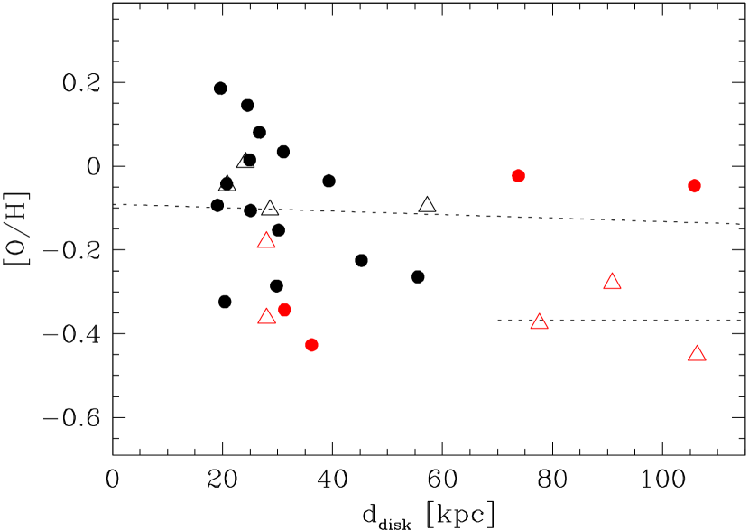
Figure 3: The O/H abundance radial gradient. Symbols are like in Figure 2. Dashed lines are described in the text.

5 M31 O/H abundance gradient

The O/H abundance radial gradient, compiled with all PNe studied in papers I and II (black symbols) and this work (red symbols), is presented in Figure 3. It extends the metallicity gradient from this type of object to galactocentric distances larger than 100 kpc, assuming that all PNe are located in the plane of the disk of M31. Sources with radial velocities consistent with the disk kinematics (V_diff$<$100 km s^-1, circles) are separated from those with large deviations from the disk kinematical model of Ibata et al. (2005, triangles). The graph shows that even at large distances PNe with solar metallicity and disk-like kinematics exist. A least-square-fit to sources with V_diff$<$100 km s^-1 provides an almost flat metallicity slope ([O/H]$=$$-0.0909$$-0.0004$$\times d_{disk}$, with $\left<[\mbox{O/H}]\right>$$=$$-0.11$). It is indicated by the upper dashed line in the figure. As a note of caution, the two PNe with solar oxygen abundance at $d_{disk}>60$ kpc are M2543 and M2566. Both are located along the minor axis of M31’s disk. Therefore their deprojection factors to the disk plane are large, and radial velocities are close to the systemic velocity of the galaxy. They do not appear to be associated with any major substructure in the halo (see also Merrett et al., 2006), although it should also be noted that that the GSS pervades a large portion of the outer regions of M31 out to 100 kpc, and its debris extend beyond the SE quadrant where it is more prominent (Ibata et al., 2014).

Figure 3 also shows that the three PNe at $d_{disk}>60$ kpc which deviate from the disk kinematics have a lower metallicity ($\left<[O/H]\right>$$=$$-0.37$, lower dashed line). This indicates that they might be related to an older population, but their only slightly subsolar O/H seemingly precludes their association with the stars in the most metal-poor and ancient component of the halo identified by e.g. Ibata et al. (2014).

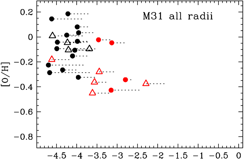
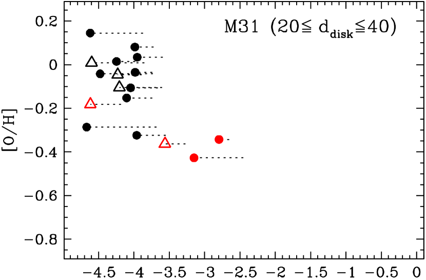
Figure 4: The O/H abundances as a function of the absolute [O III] magnitudes of PNe in M31 (top two panels, adopted distance 770 kpc) and in M33 (bottom panel, adopted distance 840 kpc). The dashed lines indicate the adopted extinction values (see text). For M31, symbols are like in Figure 2.

Before moving to a more general interpretation, two things should be noted. In this paper, we assume that the O/H abundance ratio in the PNe reflects the original oxygen content of the stellar progenitors, i.e. of the ISM from which these stars formed. There are some indication that oxygen may be enhanced in some AGB stars during the third dredge-up episodes, but this possible effect is neglected here as no clear conclusion has been drawn yet (Karakas & Lattanzio, 2014; Henry et al., 2012; Delgado-Inglada et al., 2015).

Also, it should be recalled that our target PNe were selected to be bright enough to allow an accurate chemical analysis. Indeed, all lie within 2.4 mag from the bright cutoff of the PNLF. Richer (1993) in the LMC, and Jacoby & Ciardullo (1999) in M31, suggested that there might be a slight dependence of metallicity with the [O III] luminosity, but concluded that the luminosities of the brightest PNe are nearly independent of O/H. On the other hand, Magrini et al. (2004) did not find any trend of chemical abundances as a function of the [O III] luminosity for PNe in the LMC and our Galaxy, concluding that the chemical abundances derived from the brightest PNe are representative of the total PN population. Figure 4, compiled with our data of M31, shows some tendency of decreasing metallicity with [O III] luminosity. The upper panel displays our measured O/H abundances as a function of the absolute [O III] magnitude corrected for foreground and internal extinction using the c(H$\beta$) values determined in our spectra. PNe in the brightest magnitude bin (M($5007$)$\leq$$-3.7$) have some spread in metallicity, but on average have higher O/H abundances than PNe in the next magnitude bin. To minimize the effects of the – albeit shallow – abundance gradient, the middle panel confirms that the trend persists if sources are selected in a more limited range of galactocentric distances. A similar relation is also seen seen in M33 (lower panel), where we have used the data from Magrini, Stanghellini & Villaver (2009), which were dereddened adopting the M33 foreground and internal extinction from Cepheids (Freedman et al., 2001). The decrease of mean metallicity with the [O III] luminosity may explain why the dispersion in the radial gradient of M31 at $d_{disk}<40$ kpc is increased, compared to the corresponding graphs in papers I and II, with the addition of the slightly fainter PNe presented in this work.

In a standard scenario where metallicity of a galaxy increases with time and the PN progenitors do not form or destroy oxygen, the observed correlation between luminosity and O/H content is qualitatively consistent with the hypothesis that the most luminous PNe are produced by younger, i.e. more massive progenitors than fainter PNe. The hydrodynamical simulations by Schönberner et al. (2007, see also and ) support such a view and provide further constraints to the stellar masses of our target PNe. Schönberner et al. (2007) found that only PNe with central stars masses $>$0.6 M_⊙ can attain the [O III] luminosity of the bright cutoff of the PNLF if accompanied by sufficiently delayed optically thin/thick transition of the nebular gas. Adopting the empirical initial-to-final mass relationships of Catalan et al. (2008), these relatively high core masses imply progenitors with an initial mass larger than $\sim$2 M_⊙. Our new targets are between 1 and 2 magnitudes below the PNLF cutoff. These slightly fainter magnitudes can either correspond to the most luminous PNe that have started to fade, or by PNe from slightly less massive progenitors at the their maximum luminosity. Figure 7 in Schönberner et al. (2007) shows for instance that PNe with core masses of 0.565 M_⊙ (initial masses $\sim$1.5 M_⊙) are not able to reach the [O III] luminosities of our targets. We adopt this value as the lower limit for the PN progenitors studied in this work. On the other side, it should be considered that with increasing mass the number of progenitors decreases (according to the standard IMF), and the duration of the high [O III] luminosity phase of their nebulae becomes much shorter (Schönberner et al., 2007). Therefore, statistically, it is unlikely to find very massive progenitors among our targets. A rough upper limit of $\sim$2.5 M_⊙ may be assumed, considering that none of them is a type I PN (Phillips, 2001). We conclude that the PNe presented in this work are expected to be produced by stars with masses roughly between 1.5 M_⊙ and 2.5 M_⊙. The lifetime of these stars is $\leq$3.5 Gyr. This mass range is also consistent with the modest nitrogen enhancement of the target nebulae, because the solar-metallicity models of Karakas (2010) predict significant N overabundances only for significantly more massive progenitors ($>$4 M_⊙) such as observed in some Galactic bipolar nebulae (Corradi & Schwarz, 1995).

It is important to note that our arguments are purely based on single-star evolution considerations. They do not tackle the problem that the PNLF cutoff magnitude is the same in all galaxies, even in older stellar populations where $\geq$2 M_⊙ stars are not found (Ciardullo et al., 2002; Ciardullo, 2010). This may require alternative channels of PN production to populate the bright end of the PNLF, such as mergers or mass accretion in interacting binaries (Ciardullo et al., 2005; Soker, 2006). In such case, our mass estimates would not be valid. However, low-mass progenitors would not be expected to have the high metallicity that we measure. In addition, as discussed in the next section, there is independent evidence that in the outer regions of M31 2 M_⊙ stars with solar metallicity do exist.

6 Conclusions

We have identified two PNe at very large galactocentric distances with solar oxygen abundances and radial velocities consistent with that of the extended disk of M31. Their stellar progenitors, according to single-star evolutionary theories, are estimated to be in the range 1.5–2.5 M_⊙. These two additional objects support our previous conclusion (paper II) that the luminous PNe found outside the disk of M31 trace a burst of star formation that occurred $<$3 Gyr ago. This interpretation is also fully consistent with the results of Bernard et al. (2015), who detect trace of such a recent starburst in all the HST fields studied, which span a similar galactocentric distance range as our PNe. A similar starburst of solar metallicity stars is also found throughout the disk of M31 by the Panchromatic Hubble Andromeda Treasury (Ben Williams, private communication), as well as in the outer disk of M33 (Bernard et al., 2012). The most likely explanation for the luminous oxygen-rich PNe in M31’s exodisk is that the observed, relatively massive stars found in the outer regions of M31 are part of the thin disk that has been kicked out during a recent encounter with M33, and/or following the impact with the unidentified progenitor of the Giant Stellar Stream (e.g. McConnachie et al., 2009; Bernard et al., 2012, 2015).

Three other PNe in the outer regions of M31 have O/H abundances $\sim$0.4 dex lower, and show significant deviations from the kinematics of M31’s exodisk. It is possible that they belong to one or another of the halo’s substructures discussed in the literature. No bona fide PN belonging to the smooth, mostly metal-poor, ancient halo described by Ibata et al. (2014) has been found yet. Nor would this be expected since the ancient PNe will be far fainter than the younger ones. Assuming a total luminosity of the smooth halo component of $\sim$10^-9 L_⊙ (Ibata et al., 2014) and a luminosity-specific PN number of $\sim$10^-7 (Buzzoni, Arnaboldi, & Corradi, 2006), some 10² halo PNe are expected, but only a tenth of them within two magnitudes from the bright cutoff of the PNLF, which is the luminosity range that we have explored so far. The number could be even smaller considering that, in old stellar populations, AGB stars with core masses $\leq$0.55 M_⊙ may not produce PNe, either because the post-AGB evolution of the core is too slow to “light up” the nebulae before they disperse, or because stars escape the AGB phase (Buzzoni, Arnaboldi, & Corradi, 2006).

Given the complexity of the outer regions of M31 and the small number of PNe available, our interpretation should be considered as speculative. However, it fits well into the modern view of a rich interaction and merger history for M31, providing independent support to the results obtained using other classes of stars, and adding complementary information about chemical elements that are best studied in ionized nebulae.

Appendix A Flux measurements and computed properties

Table 2 lists the emission-line measurements of all observed PNe. Column entries are as follows: the first column lists the ion and wavelength designation of each line; f($\lambda$) gives the value of the reddening function, normalized to H$\beta$ = 0; and the following lines show the measured flux relative to H$\beta$ = 100. At the bottom of each column, for each nebula we list the log of the total observed H$\beta$ flux through the spectrograph slit. Note that the latter may differ from the magnitude in Merrett et al. (2006), as not all observations were obtained in photometric nights and no attempt was done to account for slit slosses. Table 3 contains the logarithmic reddening parameter, c(H$\beta$), and the derived $N_{e}$ and $T_{e}$ of each nebula and the corresponding diagnostics. Tables 4–6 display their ionic abundances. They also show the temperatures adopted from Table 3 that were used to calculate them. Asterisks denote values that were used in the brightness-weighted mean values (wm) in lines below them. Also included for each elements is the derived ionization correction factor (icf), calculated as described in Kwitter & Henry (2001). Table 7 lists the total abundances. Note that the ELSA code determines uncertainties in the dereddened line intensities including the uncertainty in c(H$\beta$). Uncertainties in temperature and density diagnostics incorporate the errors in their constituent lines, and ionic abundance uncertainties include errors in the relevant line intensities, temperature, and density. Final abundances incorporate errors in the ionic abundances, but not on the icf. For more details, see for example Milingo et al. (2010). Note also that the calculation of a reliable sulfur abundance with the adopted icf scheme requires the measurement of S²⁺, that is estimated to be significantly more abundant than S⁺ in all targets. Therefore, in the cases where no S²⁺ lines could be measured we do not quote the S/H and S/O total abundances.

Table 2: Line identification and observed fluxes

Ident.	f($\lambda$)	M2507	M2538	M2539	M2541	M2543	M2549	M2566	M2988	M31-372
[O II] $\lambda$ 3727	0.292	24.8	61.5	20.9	33.1	26.8	27.4	84.9	27.1	$\cdots$
He ii+H9  $\lambda$ 3835	0.262	4.55	$\cdots$	6.03	$\cdots$	$\cdots$	$\cdots$	$\cdots$	$\cdots$	$\cdots$
[Ne III] $\lambda$ 3869	0.252	44.2	107	84.9	61.9	93.1	94.9	108	68.2	48.3
He i+H8  $\lambda$ 3889	0.247	13.8	8.83:	16.7	15.1	16.0	17.6	19.5	13.2	18.8
[Ne III]+H$\epsilon$  $\lambda$ 3968	0.225	28.9	33.0:	36.4	36.8	42.3	46.5	51.5	34.2	34.1
He i+He ii $\lambda$ 4026	0.209	$\cdots$	$\cdots$	2.22	$\cdots$	$\cdots$	$\cdots$	$\cdots$	$\cdots$	$\cdots$
[S II] $\lambda$ 4071	0.196	$\cdots$	$\cdots$	1.24	$\cdots$	$\cdots$	4.76	3.56	$\cdots$	$\cdots$
He ii $\lambda$ 4100	0.188	$\cdots$	0.116	$\cdots$	0.435	$\cdots$	0.308	6.26(-2)	$\cdots$	$\cdots$
H$\delta$  $\lambda$ 4101	0.188	24.3	29.3	$\cdots$	25.2	$\cdots$	25.0	25.8	$\cdots$	22.6
He ii $\lambda$ 4339	0.124	$\cdots$	0.215	2.27(-2)	0.775	0.105	0.557	0.113	$\cdots$	$\cdots$
H$\gamma$  $\lambda$ 4340	0.124	44.5	46.4	46.0	43.2	45.0	44.2	43.5	48.6	42.2
[O III] $\lambda$ 4363	0.118	6.39	18.6	12.9	13.5	8.33	16.0	8.90	9.96	10.3
He i $\lambda$ 4472	0.090	4.30	7.63::	4.91	4.21	5.66	3.79	5.32	5.35	6.05
He ii $\lambda$ 4542	0.072	$\cdots$	$\cdots$	$\cdots$	1.62	$\cdots$	$\cdots$	$\cdots$	$\cdots$	$\cdots$
N III+O II $\lambda$ 4640	0.048	$\cdots$	$\cdots$	$\cdots$	1.14	$\cdots$	2.70	$\cdots$	$\cdots$	$\cdots$
C III+O II $\lambda$ 4650	0.045	$\cdots$	$\cdots$	$\cdots$	0.901	$\cdots$	$\cdots$	$\cdots$	$\cdots$	$\cdots$
He ii $\lambda$ 4686	0.036	$\cdots$	12.1:	0.971	32.5	4.62	23.8	4.95	$\cdots$	$\cdots$
He i+[Ar IV] $\lambda$ 4711	0.030	$\cdots$	$\cdots$	$\cdots$	2.44	$\cdots$	4.39	3.69	$\cdots$	$\cdots$
[Ar IV] $\lambda$ 4740	0.023	$\cdots$	4.41	2.46	1.69	5.48	4.53	3.43	$\cdots$	$\cdots$
He ii $\lambda$ 4859	0.000	$\cdots$	0.488	4.85(-2)	1.62	0.226	1.20	0.242	$\cdots$	$\cdots$
H$\beta$  $\lambda$ 4861	0.000	100	100	100	100	100	100	100	100	100
He i $\lambda$ 4922	-0.021	1.10	$\cdots$	1.38	1.18	$\cdots$	$\cdots$	$\cdots$	$\cdots$	$\cdots$
[O III] $\lambda$ 4959	-0.030	232	479	378	324	418	415	427	311	324
[O III] $\lambda$ 5007	-0.042	697	1498	1140	978	1270	1243	1302	948	985
[Fe VI] $\lambda$ 5147	-0.074	$\cdots$	$\cdots$	0.421	$\cdots$	$\cdots$	$\cdots$	$\cdots$	$\cdots$	$\cdots$
He ii $\lambda$ 5412	-0.134	$\cdots$	$\cdots$	$\cdots$	2.88	$\cdots$	1.79	$\cdots$	$\cdots$	$\cdots$
[Cl III] $\lambda$ 5538	-0.161	$\cdots$	$\cdots$	0.466	$\cdots$	$\cdots$	$\cdots$	$\cdots$	$\cdots$	$\cdots$
[N II] $\lambda$ 5755	-0.207	1.24	$\cdots$	0.755	$\cdots$	$\cdots$	$\cdots$	1.30	$\cdots$	$\cdots$
He i $\lambda$ 5876	-0.231	16.8	18.8::	17.8	12.3	17.9	13.7	17.2	19.4	17.0
[O I] $\lambda$ 6300	-0.313	2.41	$\cdots$	2.95	3.41	$\cdots$	$\cdots$	$\cdots$	5.26	$\cdots$
He ii $\lambda$ 6311	-0.315	$\cdots$	$\cdots$	$\cdots$	0.123	$\cdots$	$\cdots$	$\cdots$	$\cdots$	$\cdots$
[S III] $\lambda$ 6312	-0.315	1.67	$\cdots$	1.08	1.07	$\cdots$	$\cdots$	$\cdots$	$\cdots$	$\cdots$
[O I] $\lambda$ 6364	-0.325	0.753	$\cdots$	1.17	0.854	$\cdots$	$\cdots$	$\cdots$	2.15	$\cdots$
[N II] $\lambda$ 6548	-0.358	9.52	33.6::	7.35	8.42	9.48	8.48	27.6	9.89	5.22
He ii $\lambda$ 6560	-0.360	$\cdots$	1.79	0.146	4.65	0.702	3.68	0.742	$\cdots$	$\cdots$
H$\alpha$  $\lambda$ 6563	-0.360	326	331	311	295	319	318	314	357	334
[N II] $\lambda$ 6584	-0.364	27.9	80.0	21.4	24.2	26.6	26.5	85.4	27.8	15.5
He i $\lambda$ 6678	-0.380	4.34	$\cdots$	4.60	3.32	4.77	3.92	4.85	5.07	4.79
[S II] $\lambda$ 6716	-0.387	0.758	$\cdots$	0.717	1.69	2.22	1.99	10.6	1.03	$\cdots$
[S II] $\lambda$ 6731	-0.389	1.56	$\cdots$	1.12	2.66	3.00	2.90	14.9	1.50	$\cdots$
He i $\lambda$ 7065	-0.443	10.9	$\cdots$	11.0	5.29	7.27	6.25	6.13	11.6	8.22
[Ar III] $\lambda$ 7136	-0.453	10.4	17.7::	10.8	5.37	16.6	10.0	22.1	9.09	6.38
He i $\lambda$ 7281	-0.475	1.24	$\cdots$	$\cdots$	$\cdots$	$\cdots$	$\cdots$	$\cdots$	$\cdots$	$\cdots$
[O II] $\lambda$ 7324	-0.481	18.9	$\cdots$	7.91	5.58	4.42	5.27	8.61	11.8	6.95
[Ar III] $\lambda$ 7751	-0.539	2.77	$\cdots$	2.34	$\cdots$	3.97	3.66	4.89	2.04	$\cdots$
[S III] $\lambda$ 9532	-0.632	$\cdots$	148::	$\cdots$	$\cdots$	$\cdots$	$\cdots$	$\cdots$	$\cdots$	$\cdots$
$\log$ F(H$\beta$)		-15.05	-15.05	-15.12	-15.23	-15.26	-15.26	-15.26	-15.31	-15.64

Table 3: Extinction, electron temperatures and densities

	M2507		M2538		M2539		M2541		M2543
c(H$\beta$)	0.17		0.18		0.12		0.06		0.13
$T_{e}$([O III])	11300	$\pm$650	12700	$\pm$750	12250	$\pm$700	13150	$\pm$800	10250	$\pm$500
$T_{e}$([N II])	16000	$\pm$4450	10300		15950	$\pm$1750	10300		10300
$T_{e}$([O II])							21950	$\pm$18100
$T_{e}$([S II])
$N_{e}$([S II])	12200	${}^{+14750}_{-12200}$	10000		3000	$\pm$1600	3050	$\pm$1650	1650	$\pm$800
	M2549		M2566		M2988		M31-372
c(H$\beta$)	0.15		0.12		0.29		0.19
$T_{e}$([O III])	12950	$\pm$800	10350	$\pm$500	12250	$\pm$700	11950	$\pm$650
$T_{e}$([N II])	10300		10400	$\pm$700	12350	$\pm$350	12200	$\pm$350
$T_{e}$([O II])			14350	$\pm$5850
$T_{e}$([S II])			10250	$\pm$3500
$N_{e}$([S II])	2300	$\pm$1150	1900	$\pm$950	2250	$\pm$1100	10000

Table 4: Ionic Abundances

Ion	Tused	Abundance
		M2507		M2538		M2539
He+	[O III]	9.85	$\pm$1.32(-2)	0.103	$\pm$0.052	0.112	$\pm$0.015
He+2				1.13	$\pm$0.36(-2)	9.04	$\pm$1.34(-4)
icf(He)		1.00		1.00		1.00
O0(6300)	[N II]	∗1.26	$\pm$0.75(-6)			∗1.48	$\pm$0.42(-6)
O0(6363)	[N II]	∗1.23	$\pm$0.73(-6)			∗1.82	$\pm$0.53(-6)
O0	wm	1.25	$\pm$0.74(-6)			1.57	$\pm$0.44(-6)
O+(3727)	[N II]	∗7.56	$\pm$9.57(-6)	∗4.79	$\pm$1.01(-5)	∗3.06	$\pm$1.01(-6)
O+(7325)	[N II]	∗1.29	$\pm$0.78(-5)			∗7.96	$\pm$3.27(-6)
O+	wm	9.88	$\pm$8.30(-6)			4.41	$\pm$1.25(-6)
O+2(5007)	[O III]	∗1.65	$\pm$0.43(-4)	∗2.47	$\pm$0.64(-4)	∗2.08	$\pm$0.53(-4)
O+2(4959)	[O III]	∗1.59	$\pm$0.34(-4)	∗2.29	$\pm$0.48(-4)	∗2.00	$\pm$0.41(-4)
O+2(4363)	[O III]	∗1.65	$\pm$0.43(-4)	∗2.47	$\pm$0.64(-4)	∗2.08	$\pm$0.53(-4)
O+2	wm	1.63	$\pm$0.40(-4)	2.43	$\pm$0.59(-4)	2.06	$\pm$0.49(-4)
icf(O)		1.00		1.11	$\pm$0.07	1.01	$\pm$0.00
Ar+2(7135)	[O III]	∗6.20	$\pm$1.44(-7)	∗8.14	$\pm$4.42(-7)	∗5.67	$\pm$1.34(-7)
Ar+2(7751)	[O III]	∗6.58	$\pm$1.69(-7)			∗4.98	$\pm$1.30(-7)
Ar+2	wm	6.28	$\pm$1.44(-7)			5.55	$\pm$1.30(-7)
Ar+3(4740)				∗3.91	$\pm$0.72(-7)	∗2.72	$\pm$0.52(-7)
icf(Ar)		1.06	$\pm$0.05	1.29	$\pm$0.09	1.03	$\pm$0.01
Cl+2(5537)						∗3.29	$\pm$0.67(-8)
icf(Cl)						1.01	$\pm$0.00
N+(6584)	[N II]	∗2.60	$\pm$1.23(-6)	∗1.16	$\pm$0.20(-5)	∗1.76	$\pm$0.44(-6)
N+(6548)	[N II]	∗2.61	$\pm$1.20(-6)	∗1.44	$\pm$0.74(-5)	∗1.78	$\pm$0.39(-6)
N+(5755)	[N II]	∗2.60	$\pm$1.23(-6)			∗1.76	$\pm$0.44(-6)
N+	wm	2.61	$\pm$1.21(-6)	1.24	$\pm$0.30(-5)	1.76	$\pm$0.41(-6)
icf(N)		17.5	$\pm$12.83	6.72	$\pm$1.48	48.2	$\pm$14.76
Ne+2(3869)	[O III]	∗3.11	$\pm$0.77(-5)	∗5.01	$\pm$1.22(-5)	∗4.33	$\pm$1.04(-5)
Ne+2(3967)	[O III]	6.68	$\pm$1.62(-5)	5.05	$\pm$1.88(-5)	6.12	$\pm$1.45(-5)
icf(Ne)		1.05	$\pm$0.06	1.33	$\pm$0.11	1.02	$\pm$0.01
S+	[N II]	∗7.32	$\pm$7.97(-8)			∗2.73	$\pm$0.84(-8)
S+(6716)	[N II]	7.31	$\pm$8.04(-8)			2.70	$\pm$0.84(-8)
S+(6731)	[N II]	7.33	$\pm$7.93(-8)			2.75	$\pm$0.84(-8)
S+	[S II]
S+2(6312)	[O III]	∗2.17	$\pm$0.59(-6)			∗1.11	$\pm$0.31(-6)
S+2(9532)	[O III]			∗3.97	$\pm$2.23(-6)
icf(S)		1.57	$\pm$0.48	1.24	$\pm$0.04	2.37	$\pm$0.42

Table 5: Ionic Abundances

Ion	Tused	Abundance
		M2541		M2543		M2549
He+	[O III]	7.63	$\pm$1.09(-2)	0.120	$\pm$0.015	8.42	$\pm$1.18(-2)
He+2		2.98	$\pm$0.45(-2)	4.27	$\pm$0.65(-3)	2.21	$\pm$0.33(-2)
icf(He)		1.00		1.00		1.00
O0(6300)	[N II]	∗4.52	$\pm$0.74(-6)
O0(6363)	[N II]	∗3.53	$\pm$0.58(-6)
O0	wm	4.32	$\pm$0.68(-6)
O+(3727)	[N II]	∗1.38	$\pm$0.37(-5)	∗1.29	$\pm$0.30(-5)	∗1.13	$\pm$0.28(-5)
O+(7325)	[N II]	∗2.93	$\pm$0.80(-5)	∗3.37	$\pm$0.83(-5)	∗2.81	$\pm$0.75(-5)
O+	wm	1.60	$\pm$0.26(-5)	1.58	$\pm$0.21(-5)	1.40	$\pm$0.19(-5)
O+2(5007)	[O III]	∗1.45	$\pm$0.39(-4)	∗4.13	$\pm$0.99(-4)	∗1.91	$\pm$0.50(-4)
O+2(4959)	[O III]	∗1.40	$\pm$0.30(-4)	∗3.94	$\pm$0.76(-4)	∗1.85	$\pm$0.39(-4)
O+2(4363)	[O III]	∗1.45	$\pm$0.39(-4)	∗4.13	$\pm$0.99(-4)	∗1.91	$\pm$0.50(-4)
O+2	wm	1.44	$\pm$0.35(-4)	4.09	$\pm$0.91(-4)	1.89	$\pm$0.46(-4)
icf(O)		1.39	$\pm$0.08	1.03	$\pm$0.01	1.26	$\pm$0.05
Ar+2(7135)	[O III]	∗2.59	$\pm$0.62(-7)	∗1.29	$\pm$0.29(-6)	∗4.55	$\pm$1.09(-7)
Ar+2(7751)	[O III]			∗1.24	$\pm$0.31(-6)	∗6.68	$\pm$1.77(-7)
Ar+2	wm			1.28	$\pm$0.28(-6)	5.12	$\pm$1.22(-7)
Ar+3(4740)		∗1.56	$\pm$0.31(-7)	∗1.03	$\pm$0.19(-6)	∗4.47	$\pm$0.86(-7)
icf(Ar)		1.50	$\pm$0.09	1.07	$\pm$0.01	1.34	$\pm$0.06
Cl+2(5537)
icf(Cl)
N+(6584)	[N II]	∗3.45	$\pm$0.60(-6)	∗4.49	$\pm$0.71(-6)	∗3.53	$\pm$0.61(-6)
N+(6548)	[N II]	∗3.52	$\pm$0.61(-6)	∗4.72	$\pm$0.73(-6)	∗3.33	$\pm$0.57(-6)
N+(5755)	[N II]
N+	wm	3.47	$\pm$0.57(-6)	4.55	$\pm$0.65(-6)	3.48	$\pm$0.57(-6)
icf(N)		13.9	$\pm$2.53	27.8	$\pm$5.59	18.3	$\pm$3.28
Ne+2(3869)	[O III]	∗2.39	$\pm$0.59(-5)	∗9.43	$\pm$2.18(-5)	∗4.04	$\pm$0.99(-5)
Ne+2(3967)	[O III]	4.70	$\pm$1.14(-5)	1.41	$\pm$0.32(-4)	6.51	$\pm$1.57(-5)
icf(Ne)		1.52	$\pm$0.11	1.07	$\pm$0.01	1.34	$\pm$0.07
S+	[N II]	∗1.09	$\pm$0.28(-7)	∗1.32	$\pm$0.25(-7)	∗1.05	$\pm$0.24(-7)
S+(6716)	[N II]	1.10	$\pm$0.28(-7)	1.32	$\pm$0.25(-7)	1.06	$\pm$0.24(-7)
S+(6731)	[N II]	1.08	$\pm$0.28(-7)	1.32	$\pm$0.25(-7)	1.04	$\pm$0.24(-7)
S+	[S II]
S+2(6312)	[O III]	∗8.88	$\pm$2.65(-7)
S+2(9532)	[O III]
icf(S)		1.44	$\pm$0.08	1.77	$\pm$0.17	1.57	$\pm$0.11

Table 6: Ionic Abundances

Ion	Tused	Abundance
		M2566		M2988		M31-372
He+	[O III]	0.116	$\pm$0.015	0.115	$\pm$0.015	9.73	$\pm$1.28(-2)
He+2		4.57	$\pm$0.69(-3)
icf(He)		1.00		1.00		1.00
O0(6300)	[N II]			∗4.05	$\pm$0.82(-6)
O0(6363)	[N II]			∗5.13	$\pm$1.06(-6)
O0	wm			4.36	$\pm$0.84(-6)
O+(3727)	[N II]	∗3.98	$\pm$1.20(-5)	∗7.50	$\pm$1.89(-6)
O+(7325)	[N II]	∗6.03	$\pm$2.59(-5)	∗2.58	$\pm$0.85(-5)	∗1.16	$\pm$0.32(-5)
O+	wm	4.17	$\pm$1.16(-5)	1.30	$\pm$0.27(-5)
O+2(5007)	[O III]	∗4.10	$\pm$0.99(-4)	∗1.72	$\pm$0.44(-4)	∗1.96	$\pm$0.50(-4)
O+2(4959)	[O III]	∗3.90	$\pm$0.75(-4)	∗1.64	$\pm$0.34(-4)	∗1.88	$\pm$0.38(-4)
O+2(4363)	[O III]	∗4.10	$\pm$0.99(-4)	∗1.72	$\pm$0.44(-4)	∗1.96	$\pm$0.50(-4)
O+2	wm	4.05	$\pm$0.90(-4)	1.70	$\pm$0.41(-4)	1.94	$\pm$0.46(-4)
icf(O)		1.04	$\pm$0.01	1.00		1.00
Ar+2(7135)	[O III]	∗1.70	$\pm$0.38(-6)	∗4.05	$\pm$0.96(-7)	∗3.34	$\pm$0.77(-7)
Ar+2(7751)	[O III]	∗1.52	$\pm$0.38(-6)	∗3.56	$\pm$0.93(-7)
Ar+2	wm	1.67	$\pm$0.37(-6)	3.96	$\pm$0.93(-7)
Ar+3(4740)		∗6.22	$\pm$1.13(-7)
icf(Ar)		1.14	$\pm$0.04	1.08	$\pm$0.01	1.06	$\pm$0.01
Cl+2(5537)
icf(Cl)
N+(6584)	[N II]	∗1.43	$\pm$0.35(-5)	∗2.65	$\pm$0.52(-6)	∗1.84	$\pm$0.35(-6)
N+(6548)	[N II]	∗1.36	$\pm$0.29(-5)	∗2.79	$\pm$0.54(-6)	∗1.82	$\pm$0.34(-6)
N+(5755)	[N II]	∗1.43	$\pm$0.35(-5)
N+	wm	1.41	$\pm$0.33(-5)	2.69	$\pm$0.49(-6)	1.83	$\pm$0.33(-6)
icf(N)		11.1	$\pm$3.23	14.0	$\pm$1.87	17.8	$\pm$3.62
Ne+2(3869)	[O III]	∗1.04	$\pm$0.24(-4)	∗3.86	$\pm$0.93(-5)	∗2.82	$\pm$0.68(-5)
Ne+2(3967)	[O III]	1.64	$\pm$0.37(-4)	6.33	$\pm$1.50(-5)	6.55	$\pm$1.54(-5)
icf(Ne)		1.14	$\pm$0.04	1.04	$\pm$0.01	1.00
S+	[N II]	∗6.58	$\pm$1.71(-7)	∗3.91	$\pm$0.94(-8)
S+(6716)	[N II]	6.58	$\pm$1.72(-7)	3.91	$\pm$0.94(-8)
S+(6731)	[N II]	6.58	$\pm$1.70(-7)	3.91	$\pm$0.95(-8)
S+	[S II]	6.77	$\pm$5.06(-7)
S+2(6312)	[O III]
S+2(9532)	[O III]
icf(S)		1.35	$\pm$0.08	1.60	$\pm$0.11

Table 7: Total Elemental Abundances

Element	M2507		M2538		M2539		M2541		M2543
He/H	9.85	$\pm$1.32(-2)	0.115	$\pm$0.053	0.113	$\pm$0.015	0.106	$\pm$0.012	0.125	$\pm$0.015
N/H	4.56	$\pm$1.67(-5)	8.36	$\pm$3.26(-5)	8.50	$\pm$2.34(-5)	4.81	$\pm$1.43(-5)	1.26	$\pm$0.37(-4)
N/O	0.264	$\pm$0.107	0.259	$\pm$0.089	0.400	$\pm$0.056	0.216	$\pm$0.047	0.288	$\pm$0.057
O/H	1.73	$\pm$0.44(-4)	3.22	$\pm$0.71(-4)	2.12	$\pm$0.50(-4)	2.22	$\pm$0.51(-4)	4.39	$\pm$0.95(-4)
Ne/H	3.26	$\pm$0.85(-5)	6.64	$\pm$1.63(-5)	4.43	$\pm$1.06(-5)	3.64	$\pm$0.93(-5)	1.01	$\pm$0.23(-4)
Ne/O	0.188	$\pm$0.031	0.206	$\pm$0.033	0.209	$\pm$0.034	0.164	$\pm$0.027	0.229	$\pm$0.036
S/H	3.52	$\pm$1.37(-6)	4.93	$\pm$2.83(-6)	2.69	$\pm$1.05(-6)	1.44	$\pm$0.46(-6)	$\cdots$	$\cdots$
S/O	2.04	$\pm$0.81(-2)	1.53	$\pm$0.88(-2)	1.27	$\pm$0.33(-2)	6.46	$\pm$1.58(-3)	$\cdots$	$\cdots$
Cl/H	$\cdots$	$\cdots$	$\cdots$	$\cdots$	3.32	$\pm$0.67(-8)	$\cdots$	$\cdots$	$\cdots$	$\cdots$
Cl/O	$\cdots$	$\cdots$	$\cdots$	$\cdots$	1.56	$\pm$0.23(-4)	$\cdots$	$\cdots$	$\cdots$	$\cdots$
Ar/H	6.66	$\pm$1.60(-7)	1.55	$\pm$0.58(-6)	8.51	$\pm$1.61(-7)	6.22	$\pm$1.05(-7)	2.49	$\pm$0.40(-6)
Ar/O	3.85	$\pm$0.81(-3)	4.81	$\pm$1.78(-3)	4.01	$\pm$0.63(-3)	2.80	$\pm$0.43(-3)	5.66	$\pm$0.80(-3)
	M2549		M2566		M2988		M31-372		Solar ref.	Orion ref.
He/H	0.106	$\pm$0.013	0.121	$\pm$0.015	0.115	$\pm$0.015	9.73	$\pm$1.28(-2)	8.50(-2)	9.70(-2)
N/H	6.36	$\pm$1.89(-5)	1.57	$\pm$0.47(-4)	3.77	$\pm$0.88(-5)	3.26	$\pm$0.70(-5)	6.76(-5)	5.37(-5)
N/O	0.248	$\pm$0.048	0.339	$\pm$0.077	0.206	$\pm$0.032	0.158	$\pm$0.026	0.138	0.100
O/H	2.57	$\pm$0.59(-4)	4.64	$\pm$0.97(-4)	1.83	$\pm$0.43(-4)	2.06	$\pm$0.48(-4)	4.89(-4)	5.37(-4)
Ne/H	5.40	$\pm$1.35(-5)	1.19	$\pm$0.27(-4)	4.03	$\pm$0.97(-5)	2.82	$\pm$0.68(-5)	8.51(-5)	1.12(-4)
Ne/O	0.210	$\pm$0.034	0.255	$\pm$0.041	0.220	$\pm$0.036	0.137	$\pm$0.022	0.174	0.209
S/H	$\cdots$	$\cdots$	$\cdots$	$\cdots$	$\cdots$	$\cdots$	$\cdots$	$\cdots$	1.32(-5)	1.66(-5)
S/O	$\cdots$	$\cdots$	$\cdots$	$\cdots$	$\cdots$	$\cdots$	$\cdots$	$\cdots$	2.70(-2)	3.09(-2)
Cl/H	$\cdots$	$\cdots$	$\cdots$	$\cdots$	$\cdots$	$\cdots$	$\cdots$	$\cdots$	3.16(-7)	2.88(-7)
Cl/O	$\cdots$	$\cdots$	$\cdots$	$\cdots$	$\cdots$	$\cdots$	$\cdots$	$\cdots$	6.46(-4)	5.36(-4)
Ar/H	1.28	$\pm$0.21(-6)	2.62	$\pm$0.45(-6)	4.26	$\pm$1.00(-7)	3.54	$\pm$0.83(-7)	2.51(-6)	4.17(-6)
Ar/O	4.99	$\pm$0.70(-3)	5.64	$\pm$0.92(-3)	2.33	$\pm$0.48(-3)	1.72	$\pm$0.36(-3)	5.13(-3)	7.77(-3)

References

- Balick et al. (2013) Balick, B., Kwitter, K. B., Corradi, R. L. M. & Henry, R. B. C. 2013, ApJ, 774, 3 (Paper II)
- Bernard et al. (2012) Bernard, E. J., Ferguson, A. M. N., Barker, M. K., et al. 2012, MNRAS, 420, 2625
- Bernard et al. (2015) Bernard, E. J., Ferguson, A. M. N., Richardson, J. C., et al. 2015, MNRAS, 446, 2789
- Buzzoni, Arnaboldi, & Corradi (2006) Buzzoni, A., Arnaboldi, M., & Corradi, R.L.M. 2006, MNRAS, 368, 877
- Catalan et al. (2008) Catalán, S., Isern, J., García–Berro, E., & Ribas, I. 2008, MNRAS, 387, 1693
- Chapman et al. (2006) Chapman, S. C., Ibata, R., Lewis, G. F., et al. 2006, ApJ, 653, 255
- Ciardullo (2010) Ciardullo, R., 2010, PASA, 27, 149
- Ciardullo et al. (2002) Ciardullo, R., Feldmeier, J. J., Jacoby, G. H., et al. 2002, ApJ, 577, 31
- Ciardullo et al. (2005) Ciardullo, R., Sigurdsson, S., Feldmeier, J. J., & Jacoby, G. H. 2005, ApJ, 629, 499
- Corradi & Schwarz (1995) Corradi, R. L. M., & Schwarz, H. E. 1995, A&A, 293, 871
- Courteau et al. (2011) Courteau, S., Widrow, L. M., McDonald, M., et al. 2011, ApJ, 739, 20
- De Vaucouleurs (1958) De Vaucouleurs, G. 1958, ApJ, 128, 465
- Delgado-Inglada et al. (2015) Delgado-Inglada, G., Rodríguez, M., Peimbert, M., Stasińska, G., & Morisset, C. 2015, MNRAS, in press
- Freedman & Madore (1990) Freedman, W.L., & Madore, B.F. 1990, ApJ, 365, 186
- Freedman et al. (2001) Freedman, W. L., Madore, B. F., Gibson, B. D., et al. 2001, ApJ, 553, 47
- Henry et al. (2012) Henry, R. B. C., Speck, A., Karakas, A. I., Ferland, G. J., & Maguire, M. 2012, ApJ, 749, 61
- Huchra, Brodie & Kent (1991) Huchra, J. P., Brodie, J. P., & Kent, S. M. 1991, ApJ, 370, 495
- Ibata et al. (2005) Ibata, R. A., Chapman, S., Ferguson, A. M. N., et al. 2005, ApJ, 634, 287
- Ibata et al. (2007) Ibata, R. A., Martin, N. F., Irwin, M., et al. 2007, ApJ, 671, 1591
- Ibata et al. (2014) Ibata, R. A., Lewis, G. F., McConnachie, A. W., et al. 2014, ApJ, 780, 128
- Jacoby & Ford (1986) Jacoby, G. H., & Ford, H. C. 1986, ApJ, 304, 490
- Jacoby & Ciardullo (1999) Jacoby, G. H., & Ciardullo, R. 1999, ApJ, 515, 169
- Johnson et al. (2006) Johnson, M. D., Levitt, J. S., Henry, R. B. C., & Kwitter, K. B. 2006, in IAU Symp. 234, Planetary Nebulae in our Galaxy and Beyond, eds. M.J. Barlow & R. Mendez (Cambridge: Cambridge Univ. Press), 439
- Kaler (1986) Kaler, J. B. 1986, ApJ, 308, 322
- Karakas (2010) Karakas, A. I. 2010, MNRAS, 403, 1413
- Karakas & Lattanzio (2014) Karakas, A. I., Lattanzio, J. C. 2014, PASA, 31, 30
- Kwitter & Henry (2001) Kwitter, B., & Henry, R. B. C. 2001, ApJ, 562, 804
- Kwitter et al. (2012) Kwitter, B., Lehman, E. M. M., Balick, B., & Henry, R. B. C. 2012, ApJ, 753, 12 (Paper I)
- Lewis et al. (2013) Lewis, G. F., Braun, R., McConnachie, A. W., et al. 2013, ApJ, 763, 4
- Magrini et al. (2004) Magrini, L., Corradi, R. L. M., Leisy, P, et al. 2004, in Asymmetrical Planetary Nebulae III: Winds, Structure and the Thunderbird, M. Meixner, J.H. Kastner, B. Balick & N. Soker eds, ASP Conf.Proc. Vol. 313, p.42
- Magrini, Stanghellini & Villaver (2009) Magrini, L., Stanghellini, L. & Villaver, E. 2009, ApJ, 696, 729
- McConnachie et al. (2009) McConnachie, A.W., Irwin, M.J., Ibata, R. A., et al. 2009, Nature, 461, 66
- Méndez et al. (2008) Méndez, R. H., Teodorescu, A. M., Schönberner, D., Jacob, R., & Steffen, M. 2008, ApJ, 681, 325
- Merrett et al. (2006) Merrett, H. R., Merrifield, M. R., Douglas, N. G., et al. 2006, MNRAS, 369, 120
- Milingo et al. (2010) Milingo, J. B., Kwitter, K. B., Henry, R. B. C., & Souza, S. P. 2010, ApJ, 711, 619
- Pagel et al. (1992) Pagel, B. E. J., Simonson, E. A., Terlevich, R. J., & Edmunds, M. G. 1992, MNRAS, 255, 325
- Peimbert & Torres-Peimbert (1983) Peimbert, M., & Torres-Peimbert, S. 1983, in Planetary Nebulae, IAU Symp. N. 103, Flower ed., p. 233
- Phillips (2001) Phillips, J.P. 2001, MNRAS, 326, 1041
- Richer (1993) Richer, M. G. 1993, ApJ, 415, 240
- Savage & Mathis (1979) Savage, B. D., & Mathis, J. S. 1979, ARA&A, 17, 73
- Schönberner et al. (2007) Schönberner, D., Jacob, R., Steffen, M., & Sandin, C. 2007, A&A, 473, 467
- Soker (2006) Soker, N. 2006, ApJ, 640, 966
- Tanaka et al. (2010) Tanaka, M., Masashi, C., Komiyama, Y., et al. 2010 ApJ, 708, 1168
- Veljanoski et al. (2014) Veljanoski, J., Mackey, A. D., Ferguson, A. M. N., et al. 2014, MNRAS, 442, 2929
- Walterbos & Kennicutt (1988) Walterbos, R., & Kennicutt, R. 1988, A&A, 198, 61
- Werk et al. (2011) Werk, J. K. et al. 2011, ApJ, 735, 71