Time-dependent Simulation and Analytical Modelling of Electronic Mach-Zehnder Interferometry with Edge-states wave packets

Abstract

We compute the exact single-particle time-resolved dynamics of electronic Mach-Zehnder interferometers based on Landau edge-states transport, and assess the effect of the spatial localization of carriers on the interference pattern. The exact carrier dynamics is obtained by solving numerically the time-dependent Schrödinger equation with a suitable 2D potential profile reproducing the interferometer design. An external magnetic field, driving the system to the quantum Hall regime with filling factor one, is included. The injected carriers are represented by a superposition of edge states and their interference pattern reproduces the results of [Y. Ji et al., Nature 422, 415 (2003)]. By tuning the system towards different regimes, we find two additional features in the transmission spectra, both related to carrier localization, namely a damping of the Aharonov–Bohm oscillations with increasing difference in the arms length, and an increased mean transmission that we trace to the energy-dependent transmittance of quantum point contacts. Finally, we present an analytical model, also accounting for the finite spatial dispersion of the carriers, able to reproduce the above effects.

I Introduction

Edge states (ESs) are chiral one-dimensional conductive channels which arise in a 2D electron gas (2DEG) in the Integer Quantum Hall regime (IQHE)Haug (1993); Ferry et al. (2009). They are essentially immune to backscattering and are characterized by very long coherence lengthsRoulleau et al. (2008). Besides their remarkable interest for basic solid-state physics and coherent electronic devices, they are ideal candidates for both the so-called “electron quantum optics”Grenier et al. (2011) and “flying qubit” implementations of quantum computing architecturesBenenti et al. (2004); Bertoni (2009).

Indeed, several attempts to demonstrate single-qubit gate operations and electronic interference in coupled quantum wires were hampered by scattering and decoherence processesRamamoorthy et al. (2007); Yamamoto et al. (2012); Bautze et al. (2014). On the other hand, experimental realizations of electronic interferometry based on edge-channel transport seem more mature, to the point of demonstrating not only single-electronJi et al. (2003); Bocquillon et al. (2012) but also two-electron interferenceNeder et al. (2007a). Also, “which-path” detectors or quantum erasersNeder et al. (2007b); Kang (2007); Dressel et al. (2012); Buscemi et al. (2012); Weisz et al. (2014) have been implemented and the formation of quantum entanglement between indistinguishable particles has been demonstratedNeder et al. (2007a); Samuelsson et al. (2004); Bocquillon et al. (2013); Ol’khovskaya et al. (2008); Rosselló et al. (2015).

While specific features of electronic Mach-Zehnder Interferometers (MZIs)Neder et al. (2006) are still under investigation and involve possibly many-particle effectsDinh et al. (2013); Rufino et al. (2013); Rosselló et al. (2015), their basic functioning can be explained in terms of stationary electron waves interference, like their more common optical counterpart. However, contrary to photons, the time that a conduction electron takes to cross the interferometer can be comparable to switching times of typical microelectronic devices, and its spatial localization can be much less than the dimensions of a single arm of the interferometer. Thus, understanding the detailed quantum dynamics of the carriers, beyond the simple plane wave model is critical for the design of novel devices based on ES transport. This is even more relevant if the device is intended to process the information encoded in a single particle at a time, a task which requires a high resolution both in time and space.

In fact, the injection of single-electron excitations that propagate along ESs has been recently demonstratedFève et al. (2007); Bocquillon et al. (2012); Fletcher et al. (2013): with a proper time modulation of the injecting pulse, they consists of Lorentzian-shaped excitations above the Fermi sea, termed levitonsLevitov et al. (1996); Keeling et al. (2006); Dubois et al. (2013). However, leviton-based MZI has not been realized experimentally so far. The majority of the literature on electron MZIs in ESs deals with electronic currentsJi et al. (2003); Neder et al. (2006, 2007b, 2007a); Weisz et al. (2014), and the prevalent theoretical models for the transport are based upon delocalized scattering statesSamuelsson et al. (2004); Kang (2007); Dressel et al. (2012); Kazymyrenko and Waintal (2008); Chung et al. (2005); Buscemi et al. (2012), with few notable exceptionsHaack et al. (2011); Gaury and Waintal (2014).

In this work we address, both from numerical and analytical points of view, the interference properties of a Mach-Zehnder device based on ES channels tuned to filling factor $\nu$=1 and quantum point contacts used as splitting elements, when the electron travelling inside it is strongly localized. We first use a numerical approach, which, unlike other recent worksKotimäki et al. (2012); Salman et al. (2013), is based upon the direct solution of the effective-mass time-dependent Schrödinger equation, in presence of an external magnetic field. The electrons travelling inside the device are localized wave packets (WPs) of ESs, and are propagated by a generalized split-step Fourier methodWeideman and Herbst (1986); Taha and Ablowitz (1984); Kramer et al. (2008). The effects of the WP size on the transport process is analyzed. Then, we develop an analytical model also accounting for the finite spatial dispersion of the carriers. The transmission coefficient of the device subject to Aharonov-Bohm (AB) oscillationsAharonov and Bohm (1959) is obtained as a function of the magnetic field and of the geometrical parameters of the interfering paths, and the results are compared with the numerical simulations. Specifically, in Section II, we describe the initial electronic wave function and the physical device used in our simulations. In Section III we give some details on the numerical algorithm that we adopt and we describe the results of the numerical simulations. Section IV is devoted to the development of an analytical model for the transport, which takes into account the energy dispersion of the wave packet. A comparison between the predictions of the latter model and the numerical simulations is then presented in Section V. Finally, the conclusions are drawn in Section VI.

II Physical system

We consider a conduction-band electron in a 2DEG on the $x$-$y$ plane, with charge $-e$ and effective mass $m^{*}$. A uniform magnetic field $\vec{B}=(0,0,B)$ is applied along the $z$ direction and a non-uniform electric field induces a local potential energy $V(x,y)$. The latter will represent the field generated by a polarized metallic gate pattern above the 2DEG that will define energetically forbidden regions. The generic Hamiltonian $\hat{H}=(-i\hbar\vec{\nabla}+e\vec{A})^{2}/(2m^{*})+V$ can be rewritten in a more explicit form by substituting the magnetic vector potential $\vec{A}$ with its expression in the Landau gauge $\vec{A}=(0,\,Bx,\,0)$. The 2D Hamiltonian for the electron in the 2DEG then reads

$$\hat{H}=-\frac{\hbar^{2}}{2m^{*}}\frac{\partial^{2}}{\partial x^{2}}-\frac{\hbar^{2}}{2m^{*}}\frac{\partial^{2}}{\partial y^{2}}-i\hbar\frac{eBx}{m^{*}}\frac{\partial}{\partial y}$$

$$+\frac{e^{2}B^{2}}{2m^{*}}x^{2}+V(x,y).$$ (1)

We adopt a single-particle approach, thus neglecting the interaction with other free electrons of the device. Our time-dependent numerical simulations and analytical model are based on Eq. (1), as we explain in the following. Before that, we must recall briefly the derivation of Landau states and of corresponding ESsJacoboni (2010).

Let us consider a region where the electric potential is invariant along $y$, i.e. $V(x,y)=V(x)$. In the Landau gauge, the Hamiltonian (1) shows an explicit translational symmetry along the $y$ direction, and the quantum evolution of the particle can be factorized along the two axes. In this case, the eigenstates of $\hat{H}$ have the form $\Psi(x,y)=\varphi(x)e^{iky}.$ In fact, the $y$-dependent part of the wave function (WF) is a plane wave, while the $x$-dependent part (which depends also on the wavevector $k$) is a solution of $\hat{H}_{L}^{eff}\varphi_{n,k}(x)=E_{n}(k)\varphi_{n,k}(x)$, with the following 1D effective Hamiltonian

$$\hat{H}_{L}^{eff}=\frac{-\hbar^{2}}{2m^{*}}\frac{\partial^{2}}{\partial x^{2}}+\frac{1}{2}m^{*}\omega_{c}^{2}\left(x-x_{0}\right)^{2}+V(x),$$ (2)

where

$$x_{0}(k)=-\frac{\hbar k}{eB},$$ (3)

and where $\omega_{c}=\frac{-eB}{m^{*}}$ is the cyclotron frequency. Note that the parameter $x_{0}$ representing the center of the effective parabolic confinement along $x$ depends on $k$, i.e. the wavevector in the $y$ direction. The discrete energy levels $E_{n}(k)$ associated with $\hat{H}_{L}^{eff}$ are the so-called Landau levels (LLs).

If $V(x)=0$, the system eigenfunctions are the well-known localised Landau states. However, if $V(x)$ is a step-like function, defining a sub-region in which the electrons are confined, the Landau states with $x_{0}$ close to the edge have higher energy, and show a finite dispersion in $k$. They become edge states, which are delocalized WFs associated with a net probability density flux, and which can act as 1D conductive channels.

Since we want to model a carrier as a propagating wave packet, beyond the delocalized scattering state model, we need to construct such WF as a proper combination of ESs, rather than considering a single ES. This is similar to representing a free electron by a minimum uncertainty wave packet rather than a plane wave, thus including a finite uncertainty in both its position and its kinetic energy. However, in our case the magnetic field couples the two directions and some care has to be taken, since the position along $x$ and the velocity along $y$ are not independent.

We suppose that the injected electron lies in the first LL and we represent it as a linear combination of ESs with $n=1$, with Gaussian weights. We choose a Gaussian shape for our initial WP since it represents a quantum particle with the minimum quantum uncertainty in both its position and momentum, and because its longitudinal spreading with the time is limited. This allows us to follow clearly the dynamics of the localized WP without substantial high-energy components forerunning the center of the WP and leading to numerical instabilities. This choice also allows the derivation of the approximated analytical model presented in Sect. IV. However, the qualitative results of our simulations do not depend on the specific shape of the initial WP. In fact, although we address the experimental regime of Ref. Ji et al., 2003 and not the propagation of levitons, as in Ref. Fève et al., 2007, we tested different shapes for the initial electron wave function: due to the superposition principle the final state will be the composition of the different scattering states taken with their initial weight. Specifically, the wave function at the initial time will be

$$\Psi_{0}(x,y) = \int dk\,F(k)\varphi_{1,k}(x)e^{iky},$$ (4)

where $F(k)$ is the Fourier transform of a 1D Gaussian function along the $y$ axis:

$$F(k) = \frac{1}{2\pi}\int dy\,e^{-iky}\frac{e^{-\frac{(y-y_{0})^{2}}{4\sigma^{2}}}e^{+ik_{0}y}}{\sqrt[4]{2\pi\sigma^{2}}}$$

$$= \sqrt[4]{\frac{\sigma^{2}}{2\pi^{3}}}e^{-\sigma^{2}(k-k_{0})^{2}}e^{-iky_{0}}.$$

This leads to a localized WF along both directions: in $y$, the Gaussian envelope gives a finite extension around the central position $y_{0}$, in $x$, the functions $\varphi_{1,k}(x)$ are always localized around $x_{0}(k)$, and the wave vector $k$ is, in turn, localized around $k_{0}$ by our choice of $F(k)$. With the initial condition Eq. (4), our simulations will be able to take into account the effects of the size $\sigma$ of the wave packet (WP) on the interference phenomena. In order to use Eq. (4), we will be careful to initialize the WP $\Psi_{0}$ where the potential $V(x,y)$ does not depend on $y$.

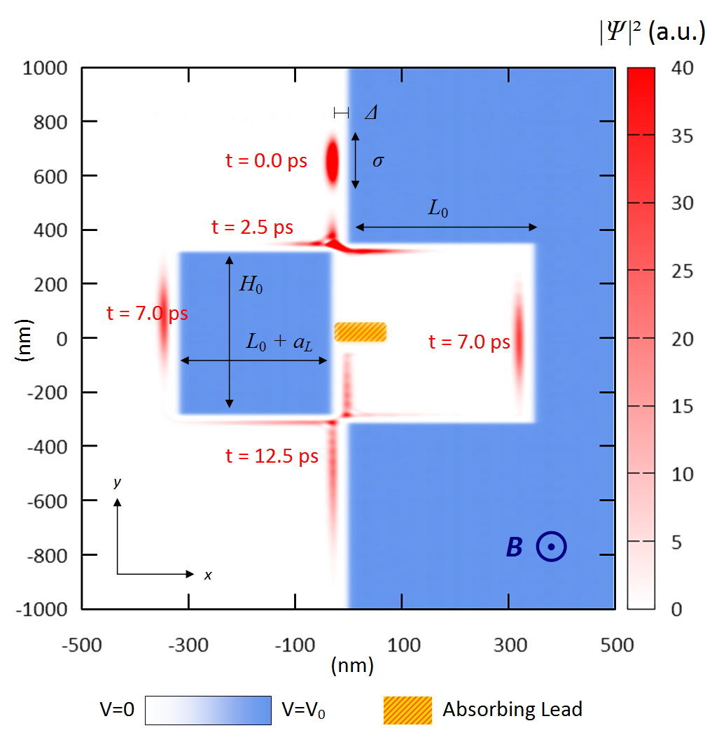
Figure 1: (Color online) Device geometry and square modulus of the WF at $t=0$ (initial state, with $\sigma=40$ nm), $t=2.5$ ps (at the first QPC), $t=7$ ps (along the two arms), $t=12.5$ ps (at the second QPC). In this example $B=5$ T and $a_{L}=-65$ nm. The resulting transmission is $T=0.599$.

The specific form of the ESs depends on the the shape of the potential barrier $V(x)$, and in general there is no closed-form expression for them. In order to have a realistic model of the smooth edges between the allowed 2DEG region and the depleted one, defined e.g. with the split-gate technique, we take

$$V(x)=V_{0}\mathcal{F}_{\tau}(x),$$ (6)

where $\mathcal{F}_{\tau}(x)=(\exp(\tau x)+1)^{-1}$ is a Fermi distribution with a “broadening” parameter $\tau$, and we compute numerically the corresponding $\varphi_{n,k}(x)$ states.

The shape of the depleted regions of our 2DEG is chosen in order to mimic, with the ES channels, the Mach-Zehnder interferometer (MZI) of Ref. Ji et al., 2003. This is depicted in Fig. 1, where the dark and light regions represent $V(x,y)=0$ and $V(x,y)=V_{0}$, respectively. Two narrowings, where two areas with high potential are close to each other, form two quantum point contacts (QPCs), both with a square area of $\delta^{2}$: their dimension $\delta$ is tuned in order to give a transmissivity of $50\%$ in the two output channels. The localized electron is injected from the top of Fig. 1 (where the initial WF is centered around $x=-20$ nm and $y=700$ nm), in the first LL, whose ESs follow the boundary between the high- and low-potential regions. After the first QPC, each ES is split into two parts that constitute the two arms (“left” and “right”) of the interferometer. They are rejoined at the second QPC. As a consequence, the two components of the WP that follow the two arms, interfere at the second QPC. Indeed, two outputs are available there to the electron: one part is reflected inside the MZI, and then absorbed by a contact (modeled as an absorbing imaginary potential $V_{abs}$, as detailed later), the other part is transmitted towards the bottom of the device. The norm of the latter part gives a measure of the transmission coefficient $T$ of the device.

The geometrical parameters of the MZI are indicated in Fig. 1. Specifically, the “right” arm and the “left” arm have two horizontal sections each, of length $L_{0}$ and $L_{0}+a_{L}$, respectively. The vertical sections of the two arms have obviously the same length, $H_{0}$. The absorbing lead is modeled by a purely imaginary potentialKramer et al. (2008); Kramer (2011)

$$V_{abs}(x,y)=iV_{abs}^{0}\frac{\mathcal{F}_{\tau}(-x+x_{c})\mathcal{F}_{\tau}(x-x_{c}-\delta_{c})}{\cosh^{2}\left((y-y_{c})^{2}/d^{2}\right)},$$ (7)

where $x_{c}$ and $y_{c}$ are the coordinates of the contact, while $\delta_{c}$ and $d$ are, respectively, the contact extension along the $x$ and $y$ axes. By changing the parameters of the device, such as $a_{L}$ (which controls the relative length of the two arms and the area) or the magnetic field $B$, we observe AB oscillations in the transmission coefficient $T$. With the introduction of the absorbing lead $V_{abs}$, the calculation of $T$ is straightforward, since it is the norm of the final wave function after the absorption process. Differently to other worksGaury et al. (2014) focusing on the dynamics of carriers moving along Hall ESs, our confining potential $V$ does not depend on time.

The “center” $x_{0}(k_{0})$ of the initial WP ($t=0$) is fixed at a distance $\Delta$ from the inflection point of the potential barrier $V(x)$, and consequently $k_{0}$ can be calculated by Eq. (3). The resulting local bandstructure of the 1st LL around $k=k_{0}$ can be determined numerically, and from a parabolic fit we get the values of the parameters $E_{0}$, $m_{B}^{*}$ and $k_{1}$ in its expression:

$$E_{1}(k)=\frac{\hbar^{2}}{2m_{B}^{*}}(k-k_{1})^{2}+E_{0}.$$ (8)

The parameters $k_{0}$ and $k_{1}$ are gauge-dependent quantities, since they depend by the origin of the coordinate system: however, with a proper choice of this degree of freedom and of the energy zero, we can set $k_{1}=0$ and $E_{0}=0$ without any physical change in the description of the system, in order to get a simpler description of the system. Now $k_{0}$ is directly related to the group velocity $v_{g}=\hbar k_{0}/m_{B}^{*}$ of the WP, which behaves like a free particle of mass $m_{B}^{*}$ in 1D.

In the simulations we use for the electron the effective mass of GaAs $m^{*}=0.067\,m_{e}$. The parameters of the potential and of the absorbing contact are $V_{0}=10$ eV, $\tau^{-1}=3$ nm, $\delta_{c}=100$ nm, $d=30$ nm, $V_{abs}^{0}=-98.7$ eV; the constructive parameters of the device are $\delta=32.2$ nm, $L_{0}=350$ nm and $H_{0}=600$ nm; the parameters of the WP are $\Delta=20$ nm and $\sigma=20,40,60$ nm, while the magnetic field is kept around the value of $B=5$ T.

III Numerical simulations

The time evolution of the WP is realized with the split-step Fourier methodSerafini and Bertoni (2009); Kramer et al. (2008); Kramer (2011). In summary, the evolution operator $\hat{U}(\delta t)=e^{-\frac{i}{\hbar}\delta t\cdot\hat{H}}$ is applied $N$ times to the initial wave function $\Psi(x,y;\,0)$, each leading to the evolution of a short time step $\delta t$:

$$\Psi(x,y;\,t)|_{t=N\delta t}=[\hat{U}(\delta t)]^{N}\Psi(x,y;\,0).$$ (9)

The Hamiltonian of Eq. (1) can be written as $\hat{H}=\hat{T}_{1}(x,p_{y})+\hat{T}_{2}(p_{x})+\hat{V}(x,y)$, with

$$\hat{T}_{1}(x,p_{y})=-\frac{\hbar^{2}}{2m^{*}}\frac{\partial^{2}}{\partial y^{2}}-i\hbar\frac{eBx}{m^{*}}\frac{\partial}{\partial y}+\frac{e^{2}B^{2}}{2m^{*}}x^{2},\quad$$ (10)

$$\hat{T}_{2}(p_{x})=-\frac{\hbar^{2}}{2m^{*}}\frac{\partial^{2}}{\partial x^{2}}.\quad$$ (11)

By applying the Trotter-Suzuky factorization and the split-step Fourier method, the operator $\hat{U}(\delta t)$ can be approximated with

$$[\hat{U}(\delta t)]^{N}=e^{+\frac{i}{\hbar}\delta t\cdot\frac{\hat{V}}{2}}\left[e^{-\frac{i}{\hbar}\delta t\cdot\left(\hat{V}+\hat{V}_{abs}\right)}\mathscr{F}_{y}^{-1}e^{-\frac{i}{\hbar}\delta t\cdot\hat{T}_{1}}\mathscr{F}_{y}\mathscr{F}_{x}^{-1}e^{-\frac{i}{\hbar}\delta t\cdot\hat{T}_{2}}\mathscr{F}_{x}\right]^{N}e^{-\frac{i}{\hbar}\delta t\cdot\frac{\hat{V}}{2}},$$ (12)

where $\mathscr{F}_{x(y)}$ and $\mathscr{F}_{x(y)}^{-1}$ denote, respectively, the direct and inverse Fourier transform with respect to the variable $x(y)$. By using the above expression, the numerical solution of Eq. (9) is reduced to an alternating application of discrete Fourier transforms and array multiplications, since each operator acts only in its diagonal representation.

Within this scheme, we can reproduce the exact dynamics of the electronic WF inside the device. As an example, the evolution of the WP at four different times is shown in Fig. 1 for the specific case described in the caption. The simulations have been performed with a time-step $\delta t=0.1$ fs.

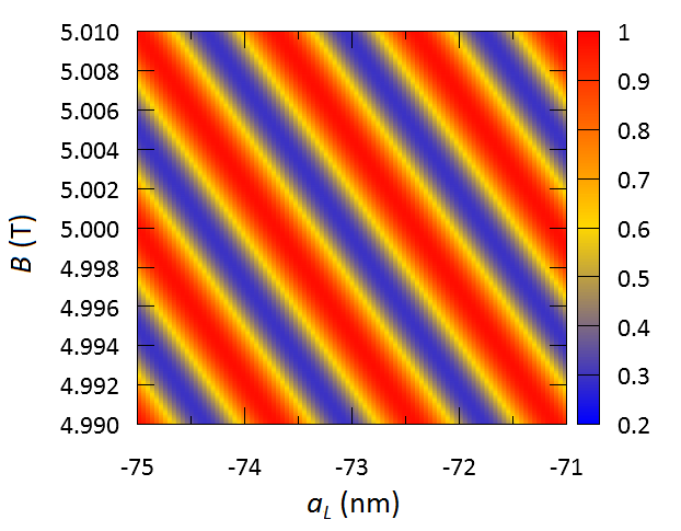
Figure 2: (Color online) Aharonov-Bohm oscillations in the transmission coefficient $T$ as a function of the asymmetry parameter of the left arm $a_{L}$ and of the magnetic field $B$ (numerical simulations for a wave packet with $\sigma=40\,\mathrm{nm}$).

As expectedJi et al. (2003); Neder et al. (2007a); Weisz et al. (2014), we obtain AB oscillations of the transmission $T$ (see Figure 2) with respect to both the variation of the area (which is controlled through $a_{L}$) and the variation of the magnetic field $B$. This is consistent with the results of Refs. Ji et al., 2003 and Neder et al., 2007a, where the tailoring of the length of one of the two paths is achieved through a modulation gate.

However, we observe two extra features, namely (a) a damping of the AB oscillations with $a_{L}$ and (b) an increase of the average $T$ as the initial spatial localization $\sigma$ of the WP is increased, with a consequent decrease of the visibilityJi et al. (2003); Neder et al. (2006, 2007b, 2007a)

$$v_{MZI}=\frac{I_{max}-I_{min}}{I_{max}+I_{min}}=\frac{T_{max}-\langle T\rangle}{\langle T\rangle}$$ (13)

of the AB oscillations (of the transmitted current $I$), which is always smaller with respect to the ideal case $v_{MZI}=1$. The two issues above are addressed in the following.

(a) The AB oscillations as a function of $a_{L}$ are modulated by a Gaussian envelope, whose extension is directly correlated with the size $\sigma$ of the initial WP. A fitting of $T$ vs $\sigma$ is reported in Fig. 3, for three values of $\sigma$ (see caption). This effect has a simple physical explanation, already advanced by Haack et al. in Haack et al., 2011 for a Lorentzian WP. Indeed, when the asymmetry between the two arms is large with respect to the size of the WP, the two parts of the WF arrive at the second QPC at different times, and do not interfere. In this case, each part is transmitted with a probability of 50%, ending up with a total transmission of $T\simeq 0.5$. In general, the larger the time offset at which the centers of the two WPs reach the second QPC, the less effective is the quantum interference. Therefore, we expect a saturation value of $\sim 0.5$ for $T(a_{L})$, and an oscillation amplitude of $\sim 0.5$. However, our numerical simulations show a different trend, i.e. issue (b).

(b) For smaller values of $\sigma$, the average (or saturation value with $a_{L}$) of the transmission $T$ is higher and the amplitude of the oscillations is lower (Fig. 3). These effects are due to the energy-dependent features of the scattering process at the QPCs, which are included automatically in the numerical simulations based on the direct solution of the Schrödinger equation. In fact, contrary to a delocalized scattering-state model, where the particle is represented by a single-energy state, our WP is composed by different ESs, as given in Eq. (4), each with a slightly different energy. As a consequence, the two parts of the WP, transmitted and reflected by the QPC, have different spectral weights, which depend on $\sigma$. Only in the limit of $\sigma\to\infty$, the WP is split into two identical parts that give an ideal $50\%$ splitting with $T=0.5$. This effect should be detectable in noise spectra of two-particle scattering, as proposed in Ref. Marian et al. (2015). In order to have a better physical insight and to give a quantitative assessment of this effect, we will include the energy-dependent transmissivity of the QPCs in the analytical model presented in the following section.

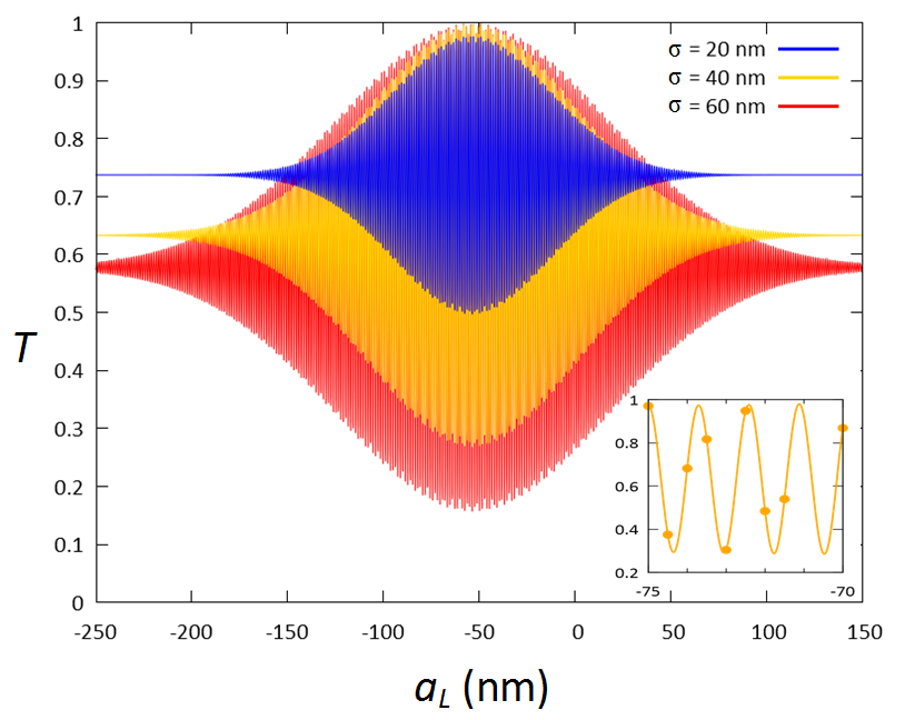
Figure 3: (Color online) Transmission coefficient $T$ as a function of the asymmetry parameter of the left arm $a_{L}$ (top curve: $\sigma=20\,\mathrm{nm}$, middle curve: $\sigma=40\,\mathrm{nm}$, bottom curve: $\sigma=60\,\mathrm{nm}$). The curves are the fits of the numerical simulation data. It turns out that the best fit is obtained with the function $T(a_{L})=c_{1}+c_{2}\cdot\exp[-c_{3}(a_{L}-c_{4})^{2}]\cdot\cos(c_{5}a_{L}+c_{6})$, where the $c_{i}$ are the fit parameters. Inset: Detail of the curve $\sigma=40\,\mathrm{nm}$ with numerical simulation data-points. All the simulations are performed at $B=5$ T.

IV Theoretical Model for the Interference

Following Weisz et alWeisz et al. (2014), we will represent a single ES as a 1D plane wave, and we will describe the scattering process and the transport inside the MZI with the scattering matrix formalismFerry et al. (2009). Of course, the effects of the scattering on the WP can be determined from the linear superposition of the scattering of single plane waves.

The device can be divided into three regions – I, II and III – as indicated in Fig. 4, where the plane-wave states are given by:

$$I. \left|D_{1}(k)\right\rangle=\left(\begin{array}[]{c}1\\ 0\end{array}\right) \left|U_{1}(k)\right\rangle=\left(\begin{array}[]{c}0\\ 1\end{array}\right),$$ (18)

$$II. \left|L(k)\right\rangle=\left(\begin{array}[]{c}1\\ 0\end{array}\right) \left|R(k)\right\rangle=\left(\begin{array}[]{c}0\\ 1\end{array}\right),$$ (23)

$$III. \left|D_{2}(k)\right\rangle=\left(\begin{array}[]{c}1\\ 0\end{array}\right) \left|U_{2}(k)\right\rangle=\left(\begin{array}[]{c}0\\ 1\end{array}\right).$$ (28)

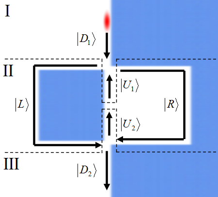
Figure 4: Scattering states inside the device. Regions I, II and III are separated with dashed lines.

The initial wave packet is prepared in the state

$$\left|\Psi_{I}\right\rangle=\int dk\,F(k)\left|D_{1}(k)\right\rangle,$$ (29)

and the scatterings at the two QPCs are described by the scattering matrices

$$S_{j}=\left(\begin{array}[]{cc}r_{j}&it_{j}\\ it_{j}&r_{j}\end{array}\right),$$ (30)

with $j=1$ ($j=2$) labeling the first (second) QPC, and where $r_{j}$ and $t_{j}$ are the transmission and reflection amplitudes. After the first QPC, the WF is given by:

$$\left|\Psi_{II}\right\rangle =S_{1}\left|\Psi_{I}\right\rangle$$

$$=\int dk\,\left(F_{L}(k)\left|L(k)\right\rangle+F_{R}(k)\left|R(k)\right\rangle\right),$$ (31)

where $F_{L}(k)=r_{1}(k)F(k)$ and $F_{R}(k)=i\,t_{1}(k)F(k)$. While travelling in the two arms of the MZI inside region II, the WF acquires a different phase in each arm, which is given byFerry et al. (2009); Heikkilä (2013); Kreisbec et al. (2010):

$$\varphi_{h}=\frac{1}{\hbar}\int_{h}(\vec{p}-q\vec{A})\cdot ds=\xi_{h}+\phi_{h},$$ (32)

where $h=L$ ($h=R$) labels the left (right) arm and the integral is a line integral along the arm $h$. The first contribution, the dynamic phase $\xi_{h}$, is due to the canonical momentum $\vec{p}$, while the second contribution, the magnetic phase $\phi_{h}$, accounts for the vector potential $\vec{A}$. The matrix describing the phase acquired is given by

$$P=\left(\begin{array}[]{cc}e^{i\varphi_{L}}&0\\ 0&e^{i\varphi_{R}}\end{array}\right),$$ (33)

and therefore the final WF in region III is given by

$$\left|\Psi_{III}\right\rangle = S_{2}P\left|\Psi_{II}\right\rangle$$ (34)

$$= \int dk\,F(k)\left(\tilde{t}\left|D_{2}(k)\right\rangle+\tilde{r}\left|U_{2}(k)\right\rangle\right),$$

where $\tilde{t}=r_{1}r_{2}e^{i\varphi_{L}}-t_{1}t_{2}e^{i\varphi_{R}}$ and $\tilde{r}=ir_{1}t_{2}e^{i\varphi_{L}}-it_{1}r_{2}e^{i\varphi_{R}}$. It is easy to see that the transmitted part of the WP is given by

$$\left|\Psi_{III}^{T}\right\rangle=\left(\frac{1}{2\pi}\int dk^{\prime}\left|D_{2}(k^{\prime})\right\rangle\left\langle D_{2}(k^{\prime})\right|\right)\left|\Psi_{III}\right\rangle,$$ (35)

where $\left\langle D_{2}(k^{\prime})|D_{2}(k)\right\rangle=2\pi\delta(k-k^{\prime})$, and therefore

$$\tilde{T} = \left\langle\Psi_{III}^{T}\middle|\Psi_{III}^{T}\right\rangle,$$ (36)

$$= 2\pi\int dk\,|F(k)|^{2}|\tilde{t}(k)|^{2}.$$

If the scattering amplitudes $r_{j}$ and $t_{j}$ are energy-independent, Eq. (36) can be integrated analytically, to give:

$$\tilde{T}=T_{0}-T_{1}e^{-\frac{\Delta l^{2}}{8\sigma^{2}}}\cos(\Delta\phi-k_{0}\Delta l),$$ (37)

where $T_{0}=\left|r_{1}r_{2}\right|^{2}+\left|t_{1}t_{2}\right|^{2}$ and $T_{1}=2r_{1}r_{2}t_{1}t_{2}$. $T_{0}$ is the mean value of the oscillations, while $T_{1}$ is their maximum amplitude. In the previous formula, $\Delta l\simeq 2a_{L}$ is the length difference between the two arms of the interferometer, while $\Delta\phi\simeq\frac{e}{\hbar}BH_{0}(a_{L_{0}}+2L)=\pi\frac{\Phi_{B}}{\Phi_{0}}$ is the well-known Aharonov-Bohm phaseFerry et al. (2009); Jacoboni (2010); Heikkilä (2013) ($\Phi_{B}$ is the flux of the magnetic field through the area of the MZI and $\Phi_{0}=\frac{h}{2e}$ is the magnetic flux quantum) .

V Discussion

As one can see, Eq. (37) provides the correct trend for the results of the simulations, with a sinusoidal oscillation enveloped by a Gaussian and with a fixed offset in the transmission. Indeed, by substituting the expressions for $\Delta\phi$ and $\Delta l$ into Eq. (37), we see that the transmission coefficient should oscillate as a function of $a_{L}$ like $\cos(k_{e}a_{L}+\varphi_{0})$, where $k_{e}=\frac{e}{\hbar}BH-2k_{0}\simeq 4.80\cdot 10^{9}\,m^{-1}$, which is consistent within 2% with the values of $k_{e}$ obtained by fitting the simulation data (see Table 1). For what concerns the amplitude and the saturation value of $T$, if we suppose that the QPCs have a perfect half-reflecting behavior for all incoming energies – that is $t_{j}=r_{j}=\frac{1}{\sqrt{2}}$ for all $k$ – then our model predicts a saturation value $T_{0}=0.5$ and an oscillation amplitude $T_{1}=0.5$, as we previously stated. This prediction, however, does not match with the numerical simulations, where we observe higher values for $T_{0}$ and lower values for $T_{1}$ (see Table 1). The model also predicts that the oscillations of $T(a_{L})$ should be modulated by a Gaussian with a standard deviation $\Sigma=\sigma$, i.e. with the same spatial dispersion of the initial wave packet. However, the actual values of $\Sigma$ obtained from numerical fitting the data of Fig. 3 are bigger than $\sigma$ by more than a factor of two in the case with smaller $\sigma$. As $\sigma$ increases, the values of $\Sigma$ (always obtained by fitting the results of the simulations) get closer to $\sigma$ (see Table 1). Indeed, a better agreement can be obtained by enhancing our model.

This simplified model is valid under certain approximations, that are: (i) the scattering process can be treated as a quasi-1D problem; (ii) all the edge channels involved in the transmission follow the same path, i.e. we can consider the area enclosed by the interfering paths and the difference in length $\Delta l$ as they were independent on $k$; (iii) the reflection and transmission amplitudes $r_{j}$ and $t_{j}$ of the QPCs are energy-independent (that means also $k$-independent). While assumptions (i) and (ii) are in general verified, the approximation (iii) must be dropped in order to reproduce the results of the simulations. Indeed, our results can be explained considering that the scattering amplitudes of the QPCs are not energy-independent, as it has been already pointed out in the literature Bocquillon et al. (2013). From a physical point of view, the edge states of higher energy are closer to the barrier, and therefore they should tunnel easier through the QPCs. This prediction can be easily verified, since the energy-dependent scattering process should produce different values in the weights $F_{L}(k)$ and $F_{R}(k)$ of the WP after the first QPC. This can be linked directly to the differences in the values of $T_{0}$ and $T_{1}$ with respect to the ideal case, as we will see briefly (a model for the correct estimation of $\Sigma$, $T_{0}$ and $T_{1}$ is given in Appendix A).

Initial WP	$T(a_{L})$ (fit)
$\sigma\;(\mathrm{nm})$	$T_{0}$	$T_{1}$	$\Sigma\;(\mathrm{nm})$	$k_{e}\;(\mathrm{nm^{-1}})$
$20.0$	0.7371	0.2403	$40.98$	$4.86$
$40.0$	0.6330	0.3650	$54.54$	$4.86$
$60.0$	0.5778	0.4215	$70.99$	$4.86$

Table 1: Data of the initial WP ($\sigma$ is the standard deviation of Eq. (II)) and the corresponding parameters for the transmission coefficient $T(a_{L})$ profile. Data were fitted with the expression $T(a_{L})=T_{0}-T_{1}\exp(-\frac{1}{2}(a_{L}-c)^{2}/\Sigma^{2})\cos(k_{e}a_{L}+\varphi_{0})$, taken from Eq. (37).

The amplitudes $t(k)$ and $r(k)$ (which are equal for both QPCs, due to their identical shape) can be calculated numerically from $\left|\Psi_{II}\right\rangle$. In Eq. (31), the squared modulus of the weights $|F_{L}(k)|^{2}$ and $|F_{R}(k)|^{2}$ has been calculated from a simulation on the wave packet with $\sigma=40\,\mathrm{nm}$ by projecting $\left|\Psi_{II}\right\rangle$ over the local eigenstates $\left|L(k)\right\rangle$ and $\left|R(k)\right\rangle$ Kramer et al. (2010). Then, using a phenomenological approach, the corresponding data have been fitted with the functions $f_{L}(k)=\mathcal{F}_{\alpha_{r}}(k-k_{r})\,|F(k)|^{2}$ and $f_{R}(k)=\mathcal{F}_{\alpha_{t}}(k-k_{t})\,|F(k)|^{2}$, thus giving a Fermi-distribution expressionBüttiker (1990) for $|r(k)|^{2}$ and $|t(k)|^{2}$. The results of the fits shown in Fig. 5 are in good agreement with the numerical simulations and are also consistent with the constraint $|r(k)|^{2}+|t(k)|^{2}=1$. From the same figure, we also deduce that the QPCs are more transparent at higher energies (i.e., lower values of $k$), as we predicted.

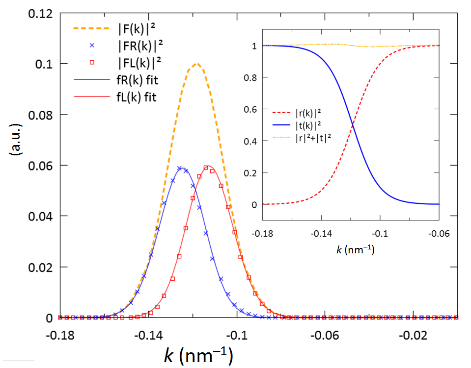
Figure 5: (Color online) Weights $|F_{R}(k)|^{2}$ and $|F_{L}(k)|^{2}$ for the transmitted and reflected part of $\left|\Psi_{II}\right\rangle$ obtained from numerical simulations ($\sigma=40\,nm$); the continuous lines are the fits with the functions $f_{R}(k)$ and $f_{L}(k)$, the dashed line is $|F(k)|^{2}$ (which is peaked on $k=k_{0}$). Inset: Squared modulus of transmission and reflection amplitudes $t(k)$ and $r(k)$ for a single QPC calculated from numerical fits.

With the hypothesis that $t(k)$ and $r(k)$ are realWeisz et al. (2014), we can insert the transmission and reflection amplitudes calculated numerically into Eq. (36) and find the exact transmission coefficient $\tilde{T}$. The results for a WP of $\sigma=20\,\mathrm{nm}$ are shown in Fig. 6: here, the simplified transmission coefficient of Eq. (37) (where $t$ and $r$ are energy-independent and both equal to $1/\sqrt{2}$) is compared with the exact energy-dependent calculation of Eq. (36), which reproduces the result of numerical simulations (see Fig. 3 for comparison). Then, as we see, the energy dependence of the scattering amplitudes $t(k)$ and $r(k)$ is able to account for the values of $T_{0}$ and $T_{1}$ and also for the broadening of $\Sigma$ (the region in which we observe interference) with respect to the original spatial extension $\sigma$ of the WP. Therefore, taking into account these corrections, it is still possible to use the simplified model of Eq. (37) to describe the interference, provided that one uses the energy-dependent values for $T_{0}$, $T_{1}$ and $\Sigma$, that we name $\tilde{T}_{0}$, $\tilde{T}_{1}$ and $\tilde{\Sigma}$. They can be calculated from our model as:

$$\tilde{T}_{0} =2\pi\int dk\,|F(k)|^{2}\left(\left|r_{1}r_{2}\right|^{2}+\left|t_{1}t_{2}\right|^{2}\right),$$ (38)

$$\tilde{T}_{1} \simeq 2\pi\int dk\,|F(k)|^{2}2r_{1}r_{2}t_{1}t_{2},$$ (39)

(see Appendix A for $\tilde{\Sigma}$ and for the details of the derivation of $\tilde{T}_{0}$ and $\tilde{T}_{1}$). In summary, we obtained an analytical formula for the visibility $v_{MZI}$ of the device, which is

$$v_{MZI}=\frac{\tilde{T}_{1}}{\tilde{T}_{0}}.$$ (40)

Indeed, we see that the device has a reduced visibility with respect to the expected ideal value $v_{MZI}=T_{1}/T_{0}=1$, due to phase-averaging effects between different energies involved in the WP (and not because of decoherence effects), as some experimental works already pointed outJi et al. (2003). Interestingly, these remarkable effects, which are comparable with experimental observations, are not explicitly related to fluctuations of the area enclosed by the two paths of the interferometer, because we used the same values of $\Delta l$ and $\Delta\phi$ for all edge states composing the WP.

As we can see from the model, in the mono-energetic plane-wave limit ($\sigma\rightarrow\infty$) the energy-dependent effects become less important, and we recover the ideal behavior with $T_{0}=T_{1}=\frac{1}{2}$ (notice that $r(k_{0})=t(k_{0})\approx\frac{1}{\sqrt{2}}$) and unitary visibility. The Gaussian modulation of the AB oscillations of the transmission coefficient disappears, since $|F(k)|^{2}\rightarrow(2\pi)^{-1}\delta(k-k_{0})$: This is consistent with scattering-states models used in the literatureJi et al. (2003); Neder et al. (2007a); Weisz et al. (2014).

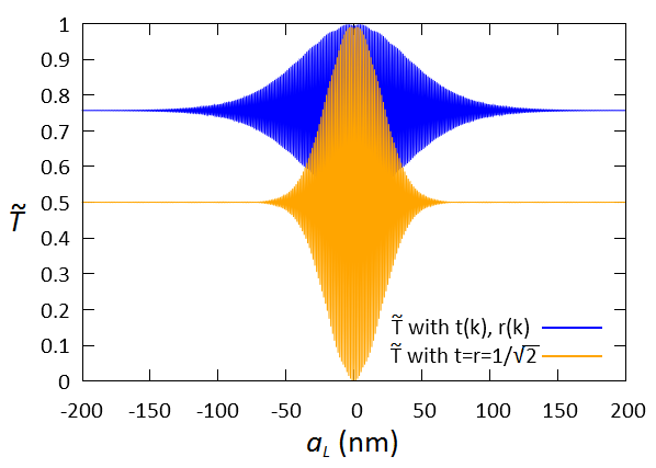
Figure 6: (Color online) Transmission coefficient $\tilde{T}$ calculated from the theoretical model for $\sigma=20\,\mathrm{nm}$, when scattering amplitudes $t=r=\frac{1}{\sqrt{2}}$ are energy-independent (Eq. (37), bottom curve) and when scattering amplitudes are energy-dependent (Eq. (36), top curve). The energy-dependent curve has $k_{e}=4.80\,\mathrm{nm}^{-1}$, $\tilde{T}_{0}=0.757$, $\tilde{T}_{1}=0.245$ and $\tilde{\Sigma}=40.4\,\mathrm{nm}$, which are very close to the results of numerical simulations (see Table 1). Note how the energy-dependent analytical model is able to reproduce the numerical results of Fig. 3 (top curve)

VI Conclusions

In conclusion, our time-dependent simulations allow us to reproduce the interference pattern of electrons transmitted through Landau edge-states defining a MZI. Specifically, we first used the split-step Fourier method to solve exactly the time-dependent Schrödinger equation, and then we calculated the single-particle dynamics and the transmission coefficient of the interferometer, which shows Aharonov-Bohm oscillations. We exposed the effects of the finite size of the electronic WP. In fact, the longitudinal extension (i.e. along the edge state) of the WP is connected to its energy uncertainty which, in turn, is determined by the injection process of the carriers: the larger the energy uncertainty, the more localized the WP. In Ref. Ji et al., 2003, for example, the carrier injection in the device is achieved by an ohmic contact operating as the source terminal. However, the specific dynamics of the electrons moving from the Fermi sea of the metallic contact to the semiconductor edge state is unknown, in general. Indeed it is strongly affected by the atomistic details of the junction, by the temperature (i.e. the broadening of the Fermi level) and, in the case of Schottky contact, by the metal-semiconductor barrier. Furthermore, if the injection of the single carrier is realized via cyclic voltage pulsesMoskalets et al. (2008); Fève et al. (2007); Hofer and Flindt (2014), its WF can be partially tailored by the pulses timing and shape, and the correlation of several carriers, possibly levitons, can be estimated as reported in Ref. Moskalets, 2015, thus assessing the transition from single-particle to multi-particle regimes.. With our approach, that includes the energy selectivity of the QPCs, the real-space spreading of the carriers can be estimated a posteriori from the interference patternHaack et al. (2011, 2013).

In addition to simulating the exact dynamics, we developed an analytical model that incorporates the physics needed to reproduce the main features of the transport spectrum. Such a model must go beyond the standard delocalized scattering-state approach. Indeed, we derived Eqs. (36) and (37) by including the effects of the finite size of the electronic WP. Furthermore, the values of $T_{0}$ and $T_{1}$ in Eq. (37) must depend on the different wave vectors $k$ composing the WP, in order to account for the energy-dependence of the scattering at the QPCs and, finally, to reproduce the offset value of the transmission, as a function of the spatial dispersion $\sigma$. Also, the model leading to Eq. (36) can justify the reduction of the visibility of the interferometer with respect to the ideal case.

Finally, we stress that the understanding of the dynamics of single electrons in Landau ESs, possibly including 4-way splittings in QPCs and a non-trivial geometry, is of utmost importance for several proposals of quantum computing architectures based on edge-channel transport. Usually, in these proposals, the quantum bits are encoded into two ESs of the same LL that are physically separated in space. However, some recent studies also focused on the possibility of coupling ESs belonging to different LLsVenturelli et al. (2011); Giovannetti et al. (2008); Devyatov (2013), between ESs belonging to two different 2DEGs through tunnelingRoddaro et al. (2013) or between spin-resolved ESs of the same LL, which could also be used in the future to realize a different type of MZIKarmakar et al. (2011, 2013) or scalable quantum gates. Also in the above systems, the effects of the spatial localization of the WP are pivotal for a realistic modeling of the devices.

Appendix A Calculation of $\tilde{\Sigma}$, $\tilde{T}_{0}$ and $\tilde{T}_{1}$

In order to give an estimate for the energy-dependent value of $\tilde{\Sigma}$, we will use a perfectly symmetrical form for $r(k)$ and $t(k)$, since the QPCs are half-reflecting for $k=k_{0}$ and $r(k)^{2}+t(k)^{2}$ must be 1 for any $k$; furthermore, we do not distinguish between QPC 1 and 2:

$$r(k) = \left[\exp(-\alpha(k-k_{0}))+1\right]^{-\frac{1}{2}}$$ (41)

$$t(k) = \left[\exp(+\alpha(k-k_{0}))+1\right]^{-\frac{1}{2}}$$ (42)

(where $\alpha=1.13\cdot 10^{-7}m$ is obtained by fitting the numerical simulations). We now replace these functions with Gaussian profiles, since near the turning point $k_{0}$ and in the decaying tail of the Fermi distribution it holds:

$$\frac{1}{\exp(\alpha(k-k_{0}))+1}\simeq\exp\!\left[-\frac{(\alpha(k-k_{0})+e)^{2}}{4e}\right]\qquad$$ (43)

(here $e$ is the Euler number). Therefore, since Eq. (36) for $r_{1}=r_{2}=r$ and $t_{1}=t_{2}=t$ can be written as

$$\tilde{T}=2\pi\int dk\,|F(k)|^{2}\times\qquad\qquad\qquad$$ (44)

$$\times\left[r(k)^{4}+t(k)^{4}+2r(k)^{2}t(k)^{2}\cos(-k\Delta l+\Delta\phi)\right],$$

we deduce that, from each term in the square brackets, we can factor out $\exp(-2\frac{\alpha^{2}}{4e}(k-k_{0})^{2})$, which can be multiplied with $|F(k)|^{2}\propto\exp(-2\sigma^{2}(k-k_{0})^{2})$ to give an “effective” Gaussian weight with an increased standard deviation. We conclude that the energy-dependent value for $\Sigma$ is given by:

$$\tilde{\Sigma}^{2}\simeq\sigma^{2}+\frac{\alpha^{2}}{4e}.$$ (45)

With this approximated model we obtain, for $\sigma=20$ nm, $\tilde{\Sigma}=39.7$ nm, which is in excellent agreement with the value $\Sigma=40.98$ nm obtained from the numerical fitting of the exact simulations (see Table 1). A similar good agreement is obtained for $\sigma=40$ nm and $\sigma=60$ nm.

Concerning the calculation of $\tilde{T}_{0}$ and $\tilde{T}_{1}$, we see from Eq. (44) that the oscillating part of $\tilde{T}$ and the Gaussian damping are given by the third term in the square brackets. Therefore, for large values of $\Delta l=2a_{L}$, the rapid oscillations of the cosine cancel out, and only the first two terms survive, to give the saturation value of the transmission. Then

$$\tilde{T}_{0} = \underset{a_{L}\rightarrow\infty}{\lim}\tilde{T}$$

$$= 2\pi\int dk\,|F(k)|^{2}\left[r(k)^{4}+t(k)^{4}\right].$$

As we did for $\tilde{T}_{0}$, we can estimate $\tilde{T}_{1}$ by comparing Eq. (44) with Eq. (37). As a first approximation, $\tilde{T}_{1}$ is the maximum amplitude of the oscillating part, which is obtained when all the oscillating functions are maximized and the Gaussian damping is zero, i.e. when the argument $\Delta\varphi$ of all the cosines in the integral vanishes (and also $\Delta l=0$). Therefore, in this limit, we can subtract the background $\tilde{T}_{0}$ from $\tilde{T}$ to get $\tilde{T}_{1}$:

$$\tilde{T}_{1} = \underset{\Delta\varphi\rightarrow 0}{\lim}\tilde{T}-\tilde{T}_{0}$$

$$= 2\pi\int dk\,|F(k)|^{2}\left[2r(k)^{2}t(k)^{2}\right].$$

For example, by using the above formulas, we obtain $\tilde{T}_{0}=0.760$ and $\tilde{T}_{1}=0.240$ for the WP with $\sigma=20$ nm, that are in good agreement wit the values of Table 1. It is straightforward to generalize these results to the cases when $r_{1}\neq r_{2}$ and $t_{1}\neq t_{2}$, to get the expressions of Eqs. (38) and (39).

Supplementary data

In this Supplementary text, we show, as an example, the dynamics of a Lorentzian wave packet crossing a QPC of the kind described into Sec. II of the main text, and compare it with the corresponding result for a Gaussian wave packet, as used in the simulations of our work.

We consider a 1D Lorentzian wave function

$$\psi_{1D}^{L}(y,t)=\frac{1}{\sqrt{\pi}}\frac{\sqrt{\frac{\Gamma}{2}}}{\left(y-y_{0}\right)-v\,t+i\,\text{sgn}(k_{F})\frac{\Gamma}{2}}e^{ik_{F}(y+v\,t)},$$

where $\Gamma$ is the full-width at middle height of the probability density $|\psi_{1D}^{L}(y,t)|^{2}$, $y_{0}$ is the position of the maximum at the initial time $t=0$. For a system with a linear dispersion $E(k)=v\cdot k$, this corresponds to the wave function of a levitonKeeling et al. (2006), but it describes also an electron emitted by a single-electron source quantum dot when subject to a suitable bias pulse Keeling et al. (2008). The imaginary exponential kinetic factor $\exp(ik_{F}(y+v\,t))$ provides the group velocity $\langle v_{g}\rangle$ corresponding to the Fermi wave vector $k_{F}$, which is given below. The factor $\text{sgn}(k_{F})$ is inserted to select only the wavevectors $k$ associated with an energy $E(k)>E_{F}$, as required by the leviton energy profile.

As in Eq. (5) of the main text, we Fourier transform in the $k$ domain in order to obtain proper weights for the ESs $\varphi(x,k)e^{iky}$

$$F^{L}(k) =\frac{1}{2\pi}\int dy\,e^{-iky}\psi_{1D}^{L}(y,0)$$ (S1)

$$=-\sqrt{\frac{\Gamma}{\sqrt{2\pi}}}ie^{-\frac{1}{2}(k-k_{F})(2iy_{0}+\Gamma\text{sgn}(k_{F}))}\Theta[(k-k_{F})\text{sgn}(k_{F})]\text{sgn}(k_{F}),$$

where we used the Heaviside function $\Theta[k]$. Therefore, the expectation value for the group velocity is:

$$\left\langle v_{g}\right\rangle=\hbar\left\langle k\right\rangle=k_{F}+\text{sgn}(k_{F})\frac{1}{\Gamma},$$

from which we can define the central wavevector $k_{0}=m\left\langle v_{g}\right\rangle/\hbar$ of the wavepacket. With the approximation that all the involved edge states have the same transverse profile (which we used also in Sect. V to derive the analytical expression for the transmission coefficient), that is $\varphi(x,k)\approx\varphi(x,k_{F})$, the 2D wavepacket becomes (see also Eq. (4) of the main text)

$$\psi^{L}(x,y) =\int dk\,F^{L}(k)\varphi_{1,k}(x)e^{iky}$$ (S2)

$$\approx\varphi(x,k_{F})\frac{e^{ik_{F}y}}{\sqrt{\pi}}\frac{\sqrt{\frac{\Gamma}{2}}}{\left(y-y_{0}\right)+i\,\text{sgn}(k_{F})\frac{\Gamma}{2}},$$

thus showing that our linear superposition of ESs has the required Lorentzian shape. The above expression (S2) is taken as the initial Lorentzian wave packet and is propagated with the numerical approach described in the main text for the Gaussian case. Supplementary Figures 1 and 2 report the square modulus of the Lorentzian and Gaussian wave functions, respectively, at the initial time and at a following time step, after the action of the QPC. The wavepackets have been initialized to have the same group velocity (numerical parameters are given in the captions). Furthermore, Supplementary Figure 3 shows the effect of the QPC energy selectivity on the Lorentzian wave function. Although the time evolution in the latter case is more noisy than in the Gaussian case described in the main text, and the spatial spreading is clearly larger, the QPC is able to split the wave packet in two parts with essentially the same integrated probability of $0.5$ but with different spectral components, as for the Gaussian case described in the main text.

List of suppfigures 1 Square modulus of the Lorentzian wave function of Eq. (S2) at the initial time (a) and at $t=6\,\text{ps}$, when the WP has been split in a reflected (b) and a transmitted (c) component by the QPC. Here $\Gamma=40\,\text{nm}$ and the wavevector $k_{0}$ associated with the group velocity is $\sim 1.2\,\text{nm}^{-1}$, while the other parameters are the same as in Fig. 1 of the main text.

List of suppfigures 2 Square modulus of the Gaussian wave function of Eq. 4 of the main text at the initial time (a) and at $t=5\text{ps}$, when the WP has been split in a reflected (b) and a transmitted (c) component by the QPC. We used the same other parameters as in Fig. 1 of the main text (i.e., $\sigma=40\,\text{nm}$ and $k_{0}\simeq 1.2\,\text{nm}^{-1}$).

List of suppfigures 3 Reciprocal-space weights, as in Eq. (S1), of the Lorentzian wave function at the initial time (yellow) and for the transmitted (blue) and reflected (red) components after the split at the QPC. Their real-space evolution is shown in Supplementary Figure 1.

References

- Haug (1993) R. Haug, Semiconductor Science and Technology 8, 131 (1993).
- Ferry et al. (2009) D. K. Ferry, S. M. Goodnick, and J. Bird, Transport in nanostructures, 2nd ed., Vol. 6 (Cambridge University Press, 2009).
- Roulleau et al. (2008) P. Roulleau, F. Portier, P. Roche, A. Cavanna, G. Faini, U. Gennser, and D. Mailly, Phys. Rev. Lett. 100, 126802 (2008).
- Grenier et al. (2011) C. Grenier, R. Hervé, G. Fève, and P. Degiovanni, Modern Physics Letters B 25, 1053 (2011).
- Benenti et al. (2004) G. Benenti, G. Casati, and G. Strini, Principles of quantum computation and information. Vol. 1: Basic concepts (World Scientific, 2004).
- Bertoni (2009) A. Bertoni, in Encyclopedia of Complexity and Systems Science, edited by R. A. Meyers (Springer New York, 2009) pp. 1011–1027.
- Ramamoorthy et al. (2007) A. Ramamoorthy, J. Bird, and J. Reno, Journal of Physics: Condensed Matter 19, 276205 (2007).
- Yamamoto et al. (2012) M. Yamamoto, S. Takada, C. Bäuerle, K. Watanabe, A. D. Wieck, and S. Tarucha, Nature nanotechnology 7, 247 (2012).
- Bautze et al. (2014) T. Bautze, C. Süssmeier, S. Takada, C. Groth, T. Meunier, M. Yamamoto, S. Tarucha, X. Waintal, and C. Bäuerle, Phys. Rev. B 89, 125432 (2014).
- Ji et al. (2003) Y. Ji, Y. Chung, D. Sprinzak, M. Heiblum, D. Mahalu, and H. Shtrikman, Nature 422, 415 (2003).
- Bocquillon et al. (2012) E. Bocquillon, F. D. Parmentier, C. Grenier, J.-M. Berroir, P. Degiovanni, D. C. Glattli, B. Plaçais, A. Cavanna, Y. Jin, and G. Fève, Phys. Rev. Lett. 108, 196803 (2012).
- Neder et al. (2007a) I. Neder, N. Ofek, Y. Chung, M. Heiblum, D. Mahalu, and V. Umansky, Nature 448, 333 (2007a).
- Neder et al. (2007b) I. Neder, M. Heiblum, D. Mahalu, and V. Umansky, Phys. Rev. Lett. 98, 036803 (2007b).
- Kang (2007) K. Kang, Phys. Rev. B 75, 125326 (2007).
- Dressel et al. (2012) J. Dressel, Y. Choi, and A. N. Jordan, Phys. Rev. B 85, 045320 (2012).
- Buscemi et al. (2012) F. Buscemi, P. Bordone, and A. Bertoni, The European Physical Journal D 66, 312 (2012).
- Weisz et al. (2014) E. Weisz, H. K. Choi, I. Sivan, M. Heiblum, Y. Gefen, D. Mahalu, and V. Umansky, Science 344, 1363 (2014).
- Samuelsson et al. (2004) P. Samuelsson, E. V. Sukhorukov, and M. Büttiker, Phys. Rev. Lett. 92, 026805 (2004).
- Bocquillon et al. (2013) E. Bocquillon, V. Freulon, J.-M. Berroir, P. Degiovanni, B. Plaçais, A. Cavanna, Y. Jin, and G. Fève, Science 339, 1054 (2013).
- Ol’khovskaya et al. (2008) S. Ol’khovskaya, J. Splettstoesser, M. Moskalets, and M. Büttiker, Phys. Rev. Lett. 101, 166802 (2008).
- Rosselló et al. (2015) G. Rosselló, F. Battista, M. Moskalets, and J. Splettstoesser, Phys. Rev. B 91, 115438 (2015).
- Neder et al. (2006) I. Neder, M. Heiblum, Y. Levinson, D. Mahalu, and V. Umansky, Phys. Rev. Lett. 96, 016804 (2006).
- Dinh et al. (2013) S. N. Dinh, D. A. Bagrets, and A. D. Mirlin, Phys. Rev. B 87, 195433 (2013).
- Rufino et al. (2013) M. J. Rufino, D. L. Kovrizhin, and J. T. Chalker, Phys. Rev. B 87, 045120 (2013).
- Fève et al. (2007) G. Fève, A. Mahé, J.-M. Berroir, T. Kontos, B. Plaçais, D. C. Glattli, A. Cavanna, B. Etienne, and Y. Jin, Science 316, 1169 (2007).
- Fletcher et al. (2013) J. D. Fletcher, P. See, H. Howe, M. Pepper, S. P. Giblin, J. P. Griffiths, G. A. C. Jones, I. Farrer, D. A. Ritchie, T. J. B. M. Janssen, and M. Kataoka, Phys. Rev. Lett. 111, 216807 (2013).
- Levitov et al. (1996) L. S. Levitov, H. Lee, and G. B. Lesovik, Journal of Mathematical Physics 37, 4845 (1996).
- Keeling et al. (2006) J. Keeling, I. Klich, and L. S. Levitov, Phys. Rev. Lett. 97, 116403 (2006).
- Dubois et al. (2013) J. Dubois, T. Jullien, F. Portier, P. Roche, A. Cavanna, Y. Jin, W. Wegscheider, P. Roulleau, and D. C. Glattli, Nature 502, 659 (2013).
- Kazymyrenko and Waintal (2008) K. Kazymyrenko and X. Waintal, Phys. Rev. B 77, 115119 (2008).
- Chung et al. (2005) V. S.-W. Chung, P. Samuelsson, and M. Büttiker, Phys. Rev. B 72, 125320 (2005).
- Haack et al. (2011) G. Haack, M. Moskalets, J. Splettstoesser, and M. Büttiker, Phys. Rev. B 84, 081303 (2011).
- Gaury and Waintal (2014) B. Gaury and X. Waintal, Nature Communications 5, 3844 (2014).
- Kotimäki et al. (2012) V. Kotimäki, E. Cicek, A. Siddiki, and E. Räsänen, New Journal of Physics 14, 053024 (2012).
- Salman et al. (2013) A. Salman, V. Kotimäki, A. Sıddıki, and E. Räsänen, The European Physical Journal B 86, 155 (2013).
- Weideman and Herbst (1986) J. A. C. Weideman and B. M. Herbst, SIAM Journal on Numerical Analysis 23, 485 (1986).
- Taha and Ablowitz (1984) T. R. Taha and M. I. Ablowitz, Journal of Computational Physics 55, 203 (1984).
- Kramer et al. (2008) T. Kramer, E. J. Heller, and R. E. Parrott, in Journal of Physics: Conference Series, Vol. 99 (IOP Publishing, 2008) p. 012010.
- Aharonov and Bohm (1959) Y. Aharonov and D. Bohm, Phys. Rev. 115, 485 (1959).
- Jacoboni (2010) C. Jacoboni, Theory of electron transport in semiconductors: A pathway from elementary physics to nonequilibrium Green functions, Vol. 165 (Springer Science & Business Media, 2010).
- Note (1) In the Supplementary data, we compare the action of a QPC on a Gaussian and a Lorentzian WP: in the second case the dynamics is more noisy and the spread larger, but the effect of the QPC energy dependence is still evident.
- Note (2) In the region of the QPCs two potential barriers with a right-angle shape face each other. The prolongation of the edges of the angles identifies a square area with side . The position of the edges is taken at the inflection point of each barrier.
- Kramer (2011) T. Kramer, AIP Conference Proceedings 1334, 142 (2011).
- Gaury et al. (2014) B. Gaury, J. Weston, and X. Waintal, Phys. Rev. B 90, 161305 (2014).
- Note (3) We choose these values for the standard deviation of the WPs because they result a good compromise for the simulations: indeed, these WPs are small enough to be localized inside the device and at the same time their time spreading is small enough to keep this condition true during all the simulation time.
- Serafini and Bertoni (2009) T. Serafini and A. Bertoni, Journal of Physics: Conference Series 193, 012049 (2009).
- Marian et al. (2015) D. Marian, E. Colomés, and X. Oriols, Journal of Physics: Condensed Matter 27, 245302 (2015).
- Heikkilä (2013) T. T. Heikkilä, The Physics of Nanoelectronics: Transport and Fluctuation Phenomena at Low Temperatures, Vol. 21 (Oxford University Press, 2013).
- Kreisbec et al. (2010) C. Kreisbec, T. Kramer, S. S. Buchholz, S. F. Fischer, U. Kunze, D. Reuter, and A. D. Wieck, Physical Review B 82, 165329 (2010).
- Note (4) The expressions for and should be corrected with two geometrical parameters and , which account for the fact that the center of the ESs channels is inside the low-potential region rather than on the allowed/forbidden region boundary, and the area encircled is not a perfect rectangle. Indeed, for , the edge states travelling in the left arm follow a longer path (external) with respect to those travelling in the right arm (internal). This is the reason why the curves obtained from numerical simulations of Fig. 3 are Gaussians which are not centered around . We should write and in order to take these effects into account. However, this gives only an offset of the length difference of the arms and does not affect the physics involved. For the sake of clarity we do not include the above expressions in the analytical derivation.
- Kramer et al. (2010) T. Kramer, C. Kreisbeck, and V. Krueckl, Physica Scripta 82, 038101 (2010).
- Büttiker (1990) M. Büttiker, Physical Review B 41, 7906 (1990).
- Moskalets et al. (2008) M. Moskalets, P. Samuelsson, and M. Büttiker, Phys. Rev. Lett. 100, 086601 (2008).
- Hofer and Flindt (2014) P. P. Hofer and C. Flindt, Phys. Rev. B 90, 235416 (2014).
- Moskalets (2015) M. Moskalets, Phys. Rev. B 91, 195431 (2015).
- Haack et al. (2013) G. Haack, M. Moskalets, and M. Büttiker, Phys. Rev. B 87, 201302 (2013).
- Venturelli et al. (2011) D. Venturelli, V. Giovannetti, F. Taddei, R. Fazio, D. Feinberg, G. Usaj, and C. A. Balseiro, Phys. Rev. B 83, 075315 (2011).
- Giovannetti et al. (2008) V. Giovannetti, F. Taddei, D. Frustaglia, and R. Fazio, Phys. Rev. B 77, 155320 (2008).
- Devyatov (2013) E. V. Devyatov, Low Temperature Physics 39, 7 (2013).
- Roddaro et al. (2013) S. Roddaro, L. Chirolli, F. Taddei, M. Polini, and V. Giovannetti, Phys. Rev. B 87, 075321 (2013).
- Karmakar et al. (2011) B. Karmakar, D. Venturelli, L. Chirolli, F. Taddei, V. Giovannetti, R. Fazio, S. Roddaro, G. Biasiol, L. Sorba, V. Pellegrini, et al., Phys. Rev. Lett. 107, 236804 (2011).
- Karmakar et al. (2013) B. Karmakar, D. Venturelli, L. Chirolli, F. Taddei, V. Giovannetti, R. Fazio, S. Roddaro, G. Biasiol, L. Sorba, L. Pfeiffer, et al., in Journal of Physics: Conference Series, Vol. 456 (IOP Publishing, 2013) p. 012019.
- Keeling et al. (2008) J. Keeling, A. V. Shytov, and L. S. Levitov, Phys. Rev. Lett. 101, 196404 (2008).