Efficient single pixel imaging in Fourier space

Abstract

Single pixel imaging (SPI) is a novel technique being able to capture 2D images using a bucket detector with high signal-to-noise ratio, wide spectrum range and low cost. Conventional SPI projects random illumination patterns to randomly and uniformly sample the entire scene’s information. Determined by the Nyquist sampling theory, SPI needs either numerous projections or high computation cost to reconstruct the target scene, especially for high-resolution cases. To address this issue, we propose an efficient single pixel imaging technique (eSPI), which instead projects sinusoidal patterns for importance sampling of the target scene’s spatial spectrum in Fourier space. Specifically, utilizing the centrosymmetric conjugation and sparsity priors of natural images’ spatial spectra, eSPI sequentially projects two $\frac{\pi}{2}$-phase-shifted sinusoidal patterns to obtain each Fourier coefficient in the most informative spatial frequency bands. eSPI can reduce requisite patterns by two orders of magnitude compared to conventional SPI, which helps a lot for fast and high-resolution SPI.

• April 2016

Keywords: single pixel imaging, computational ghost imaging, sinusoidal modulation, importance sampling

1 Introduction

Single pixel imaging (SPI) [1] is a novel incoherent imaging technique. It produces 2D images using a bucket detector instead of array sensors. SPI shares the same imaging scheme with computational ghost imaging [2], which uses a spatial light modulator (SLM) to generate programmable illumination patterns onto the target scene, and uses a bucket detector to collect the correlated lights. Then the 2D scene can be retrieved from the illumination patterns and corresponding 1D correlated single pixel measurements, using either linear correlation methods [3, 4, 5, 6] or compressive sensing (CS) techniques [7, 8]. Due to its high signal-to-noise ratio, wide spectrum range, low cost and flexible light-path configuration, SPI has been widely applied in various fields [9, 10, 11, 12].

Despite the above advantages over conventional imaging techniques using array sensors, SPI needs numerous illumination patterns to reconstruct an image, which makes it time consuming and memory demanding [13]. Such a large number of patterns is caused by the utilized random modulation, which randomly and uniformly samples all the target scene’s information with no discrimination. Determined by the Nyquist sampling theory, it needs at leat N measurements to reconstruct an N-pixel image. Especially, more measurements are needed in real applications to compensate for the system noise and the influences from other external factors. As a reference, Sun et al.[14] used around $10^{6}$ patterns (20 times of the image pixels) to reconstruct a 256$\times$192-pixel image owning sufficient quality for subsequent 3D imaging. Though one can utilize compressive sensing [7] to reduce projections, this largely increases computation complexity[8]. Instead of using random patterns, the technique recently proposed in ref. [15] utilizes sinusoidal modulation to sample the scene’s information in Fourier space. Specifically, it projects four $\frac{\pi}{2}$-phase-shifted patterns to sample each spatial frequency of the scene’s spatial spectrum, and can save a lot of projections compared to conventional SPI.

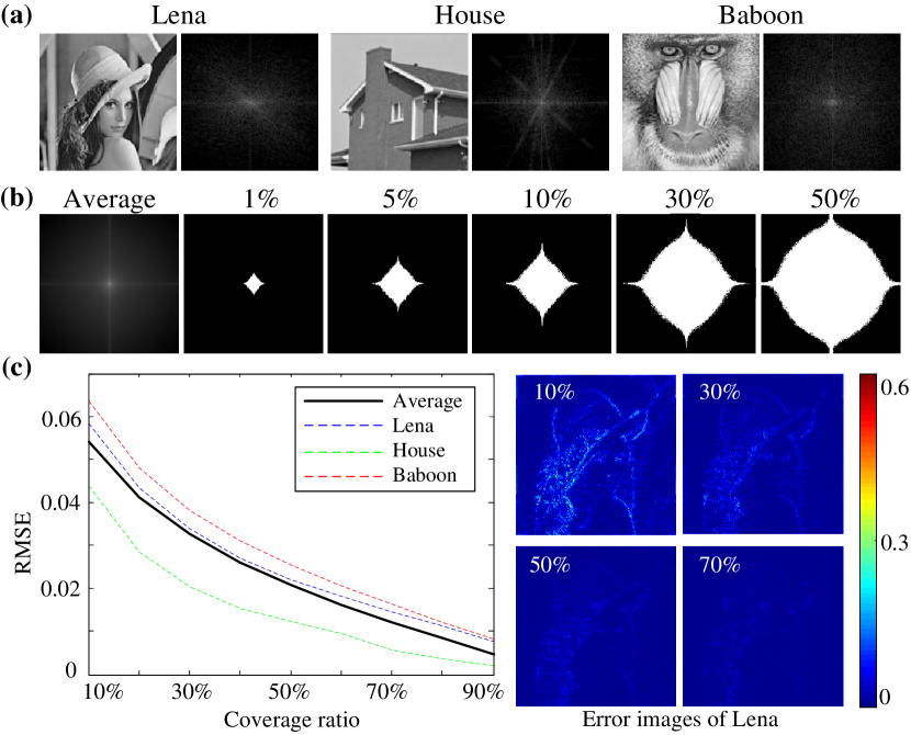
Figure 1: Statistical study of natural images’ spatial spectra. (a) Three exemplar natural images and their spatial spectra. (b) The average spectrum of the USC-SIPI database, as well as different acquisition bands under different coverage ratios. (c) The relationship between reconstruction error and coverage ratio.

From the statistics[16], most information of natural images is concentrated in low spatial frequency bands and exhibits strong sparsity in Fourier space, as shown in Fig. 1(a) where several exemplar images and their spatial spectra are presented. This motivates us to utilize the importance sampling strategy for efficient acquisition in Fourier space. To realize the non-uniform sampling of the scene’s spatial spectrum, we calculate the statistical importance distribution of nature images’ spatial frequencies and sample them in a descending order of importance. To sample each spatial frequency, since random patterns do not work anymore, we use a two-step sinusoidal illumination modulation strategy similar to ref.[17], which is based on the centrosymmetric conjugation property of real natural images’ spatial spectra. To conclude, we propose an efficient single pixel imaging technique (eSPI) in this paper. The technique utilizes the sparsity and conjugation priors of natural images’ spatial spectra to realize fast SPI with extremely high efficiency and low computation cost. We note that the proposed eSPI differentiates from ref. [15] in two aspects: (i) utilizing the sparsity prior of natural images’ spatial spectra, eSPI performs importance sampling in the Fourier domain, i.e., eSPI doesn’t sample all the Fourier coefficients exhaustively as ref. [15]; (ii) incorporating the centrosymmetric conjugation property of natural images’ spatial spectra into the patterning strategy, eSPI needs only two sinusoidal $\frac{\pi}{2}$-phase-shifted patterns for each frequency, instead of four as in ref. [15]. Benefitting from these two strategies, eSPI can save most projections of ref. [15]. In the following, we begin to introduce eSPI in two steps.

2 Methods

The first step of eSPI is to determine the acquisition band in Fourier space, i.e., to decide which Fourier coefficients to sample. Here we first study the statistical distribution of natural scenes’ spatial spectra, and accordingly determine the priority of spectrum sampling. Specifically, we transform all the 44 images in the USC-SIPI common miscellaneous database [18] to Fourier space, and calculate the spectra’s average magnitude map, as shown in the first image in Fig. 1(b). Then we threshold it to determine the acquisition bands under different coverage ratios (the ratio between the acquisition band and the whole spectrum). The results are shown in Fig. 1(b), where the white areas stand for the acquisition bands.

Based on the thresholding results, users can determine the acquisition band by setting different coverage ratios according to specific applications. Larger coverage ratio results in a wider acquisition band and more detailed information, but more projections. To further study the relationship between coverage ratio and reconstruction error, we successively sample the spatial spectrum of each image in the above dataset under different coverage ratios, transform them back to spatial space, and calculate reconstruction errors in terms of root-mean-square error (RMSE). RMSE is defined as $\sqrt{E(({\bf I}_{1}-{\bf I}_{2})^{2})}$ to measure the difference between two images ${\bf I}_{1}$ and ${\bf I}_{2}$, where $E$ is the pixel-wise average operation. The average performance is plotted as the black solid curve in Fig. 1(c), where reconstruction errors of several exemplar images are also plotted with dashed lines. The results indicate that though different images are of slight diversity, they follow the same trend that reconstruction error decreases as coverage ratio increases. Besides, the reconstruction residues of the “Lena” image at different coverage ratios are also presented as a reference.

After the acquisition band determined, we move on to the second step of eSPI, i.e., sampling each Fourier coefficient in the band to perform the non-uniform acquisition. Since random patterns do not work anymore, we use a two-step sinusoidal illumination modulation strategy similar to ref. [17] based on the centrosymmetric conjugation property of real natural images’ spatial spectra. To introduce the illumination patterning strategy in detail, we first analyze the information encoded by the single pixel measurements in Fourier space. According to the Fourier theorem, a 2D image $\bf I$ can be represented as ${\bf I}=\sum_{i}c_{i}{\bf B_{i}}$, where $\bf B_{i}$ is the $i$th normalized Fourier basis, and $c_{i}$ is its Fourier coefficient. Similarly, by applying Fourier transform to a projected pattern $\bf P$, we can get ${\bf P}=\sum_{j}\hat{c}_{j}{\bf B_{j}}$. Its corresponding single pixel measurement $s$ can be represented as

$$s = |\sum_{m}\sum_{n}{\bf I}(m,n){\bf P}(m,n)|$$

$$= |\sum_{m}\sum_{n}[\sum_{i}c_{i}{\bf B}_{i}(m,n)][\sum_{j}\hat{c}_{j}{\bf B}_{j}(m,n)]|$$

$$= |\sum_{i}\sum_{j}c_{i}\hat{c}_{j}[\sum_{m}\sum_{n}{\bf B}_{i}(m,n){\bf B}_{j}(m,n)]|.$$

Here $(m,n)$ index the 2D spatial coordinate. Substituting the orthogonality of the Fourier bases

$$f(x)=\left\{\begin{aligned} \sum_{m}\sum_{n}{\bf B}_{i}(m,n){\bf B}_{j}(m,n)&=0,&i\neq j\\ \sum_{m}\sum_{n}{\bf B}_{i}(m,n){\bf B}_{j}(m,n)&=1,&i=j,\end{aligned}\right.$$ (2)

into the above equation, we get

$$s = |\sum_{j}c_{j}\hat{c}_{j}|.$$ (3)

From this we can see that $\{\hat{c}_{j}\}$ is a spectrum sampling vector to record the scene’s Fourier coefficients. Therefore, we can directly sample a specific Fourier coefficient by setting $\{\hat{c}_{j}\}$ as a delta vector (containing only one non-zero entry), which results in a sinusoidal pattern with complex values.

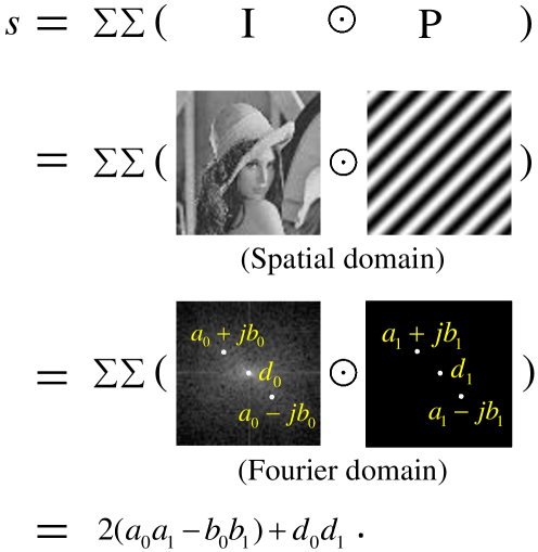
Figure 2: Illustration of the encoded information in a correlated single pixel measurement when a real valued sinusoidal pattern is projected.

However, real facilities can only project real-valued sinusoidal patterns, each owning three non-zero coefficients in its spatial spectrum—two conjugate coefficients of a centrosymmetric non-zero frequency pair and one of the zero frequency. The conjugation property also holds for natural scenes. Let $c_{1}=a_{0}+jb_{0}$, $c_{2}=a_{0}-jb_{0}$ and $c_{3}=d_{0}$ ($j$ is the imaginary unit) denote the three non-zero coefficients of the target scene $\bf I$, and $\hat{c}_{1}=a_{1}+jb_{1}$, $\hat{c}_{2}=a_{1}-jb_{1}$ and $\hat{c}_{3}=d_{1}$ represent corresponding coefficients of a sinusoidal pattern $\bf P$, we have

$$s\! = \!|c_{1}\hat{c}_{1}+c_{2}\hat{c}_{2}+c_{3}\hat{c}_{3}|$$

$$= \!|(a_{0}\!+\!jb_{0})(a_{1}\!+\!jb_{1})+(a_{0}\!-\!jb_{0})(a_{1}\!-\!jb_{1})+d_{0}d_{1}|$$

$$= \!2(a_{0}a_{1}-b_{0}b_{1})+d_{0}d_{1}.$$

A more explicit demonstration is shown in Fig. 2. Note that if the pattern’s pixel number in each dimension is even, determined by the symmetry property of discrete Fourier transform, there is no corresponding centrosymmetric counterpart of the highest spatial frequency, i.e., the highest frequency cannot form a conjugation frequency pair.

Based on the above derivations, acquiring a specific Fourier coefficient turns into computing $a_{0}$ and $b_{0}$, with $s,a_{1},b_{1}$ and $d_{1}$ known. To achieve this, we sequentially project three patterns onto the target scene. The first one is a uniform pattern with the constant intensity equal to the mean pixel value of $\bf P$, and the measurement is exactly $d_{0}d_{1}$. The other two patterns are sinusoidal patterns with Fourier coefficients being $\{a_{1}=\frac{1}{2},b_{1}=0,d_{1}=1\}$ and $\{a_{1}=0,b_{1}=\frac{1}{2},d_{1}=1\}$, respectively. Thus we can obtain $a_{0}$ and $b_{0}$ by simply subtracting $d_{0}d_{1}$ from the correlated measurements.

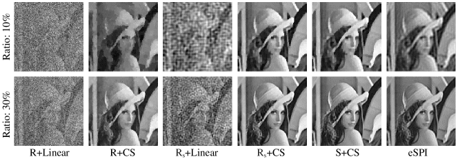
Figure 3: Simulated reconstruction results of the Lena image (128$\times 128$ pixels) by different SPI strategies, with the coverage ratio being 10$\%$ and 30$\%$, respectively. “R”, “R_s”, “S”, “Linear” and “CS” stand for random modulation, random modulation of the same speckle traverse size (same spatial frequency) as eSPI, sinusoidal modulation, linear correlation reconstruction, and compressive sensing reconstruction, respectively.

Following the above method, we can obtain all the Fourier coefficients of the pre-determined acquisition band, by sequentially projecting corresponding sinusoidal patterns (the uniform pattern needs to be projected only once for all the frequencies). Then, the target scene can be recovered by inverse Fourier transform to the obtained spatial spectrum.

3 Results

To validate the proposed eSPI technique, we first conduct a simulation experiment to compare the reconstruction performance of different SPI methods. We set the “Lena” image ($128\times 128$ and $256\times 256$ pixels respectively) as the latent target scene image, and synthesize the measurements of different patterns following Eq. 2. We set the coverage ratio being 0.1 and 0.3 (corresponding acquisition bands are shown in the fourth and fifth subfigures in Fig. 1(b)), respectively. The experiment is conducted using Matlab on an Intel i7 3.6GHz CPU computer, with 16G RAM and 64 bit Windows 7 system. For comparison, the linear correlation based reconstruction method [4, 5] and the compressive sensing based technique [1] are applied on the same set of sinusoidal patterns, as well as the same number of random patterns. Also, we compare eSPI with conventional SPI in the sense of the same speckle transverse size [12] (same spatial frequency), by truncating conventional random patterns’ spatial spectra with the same acquisition band (Fig. 1(b)) as eSPI. The results are shown in Fig. 3 and Tab. 3. Note that we omit the results of “S+Linear”, since the eSPI reconstruction (namely inverse Fourier transform) is essentially a linear combination of the Fourier bases, which is intrinsically the same as the linear correlation based method in the case of sinusoidal patterns.

Table 1: Quantitative comparison among different SPI strategies under different coverage ratios and image sizes. The ”$\times$” symbol means that the reconstruction is out of memory.

		Ratio: 10$\%$		Ratio: 30$\%$
		RMSE	Time	RMSE	Time
128$\times$128 pixels	R+Linear	0.215	2s	0.191	6s
	R+CS	0.115	68min	0.042	92min
	Rs+Linear	0.203	2s	0.187	6s
	Rs+CS	0.075	68min	0.041	91min
	S+CS	0.066	67min	0.037	92min
	eSPI	0.061	1s	0.044	3s
256$\times$256 pixels	R+Linear	0.211	9s	0.188	26s
	R+CS	$\times$	$\times$	$\times$	$\times$
	Rs+Linear	0.205	9s	0.186	25s
	Rs+CS	$\times$	$\times$	$\times$	$\times$
	S+CS	$\times$	$\times$	$\times$	$\times$
	eSPI	0.035	3s	0.014	8s

From both the visual and quantitative results, we can clearly see that eSPI largely outperforms conventional SPI in terms of both efficiency and reconstruction quality. The advantages come from the utilized sparse information encoding strategy. For conventional SPI, the spatial spectra of random patterns are also random. They sample and multiplex the target scene’s whole spectrum randomly and uniformly with no discrimination. Thus conventional SPI can not utilize the importance sampling strategy, and need much more projections for demulplexing and reconstruction. Instead, each sinusoidal pattern in eSPI only encodes a Fourier coefficient pair of the scene’s spatial spectrum. Based on this, eSPI samples only the most informative bands and omits unimportant ones. Therefore, it is much more efficient. Note that though the compressive sensing (CS) method produces similar results as eSPI when using sinusoidal patterns, it is much more time consuming and memory demanding. Especially, when image size grows large enough, CS does not work anymore. This is because CS models the reconstruction as an ill-posed problem, which needs large memory and long time for computation under an optimization framework. Instead, eSPI is linear correlation based and doesn’t involve any complex calculations, so it is much faster and memory saving.

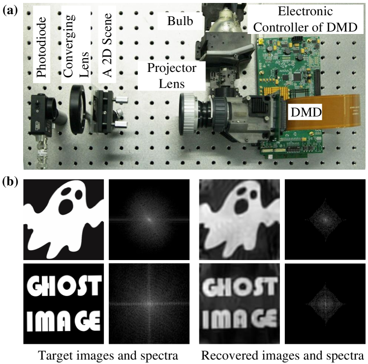
Figure 4: Experiment on real captured data. (a) The eSPI prototype. (b) Reconstruction results of two different scenes (each owning128$\times$128 pixels) with the coverage ratio being 10$\%$. The left two columns are the ground-truth target images and their spatial spectra, and the right two columns are corresponding reconstruction.

To further validate eSPI, we build a proof-of-concept prototype exhibited in Fig. 4(a). The system mainly consists of two parts including programmable illumination and detection. The illumination part includes a commercial projector’s illumination module (numerical aperture of the projector lens is 0.27) and a digital micromirror device (DMD, Texas Instrument DLP Discovery 4100 Development Kit, .7XGA) for spatial modulation. We use the 8-bit mode of the DMD to generate patterns, with the frame rate being 30Hz. Patterns owning 128$\times$128 pixels are sequentially projected onto a printed transmissive film (34mm$\times$34mm) as the target scene. Then the correlated lights are recorded by a high-speed bucket detector (Thorlabs DET100 Silicon photodiode, 340-1100 nm) with a 14-bit acquisition board ART PCI8514. The sampling rate is set as 10kHz. We utilize the self-synchronization technique in ref. [19] to synchronize the DMD and the detector. For each pattern, we average all its corresponding stable measurements for subsequent reconstruction. The coverage ratio of the acquisition band is set as $10\%$, resulting in 1635 projected patterns in total. The reconstructed results of two different scenes are shown in Fig. 4(b), from which we can see that 10$\%$ of the pixel number patterns can yield satisfying results. Compared to ref.[14] where the requisite pattern number is 20 times of the pixel number, eSPI can reduce projections by two orders of magnitude. Note that there exist some artifacts in the reconstructed images. This may be caused by several factors, including film glare, light flicker (voltage fluctuation), ambient light, modulation deviation of the DMD, thermal noise of the detector, and so on. Further efforts are needed to address these problems by improving the experimental environment and imaging elements, and proposing noise-robust reconstruction techniques.

4 Conclusion and discussion

In this paper, we propose an efficient single pixel imaging technique (eSPI). Different from conventional random illumination modulation which randomly and uniformly samples the scene’s whole spatial spectrum, eSPI uses a two-step sinusoidal illumination modulation strategy to obtain the Fourier coefficients of the target scene’s most informative spectrum band. As a result, we can reduce the requisite patterns by two orders of magnitude. This helps a lot for fast and high resolution SPI.

Figure 5: Demonstration of eSPI’s advantages for high resolution imaging. (a) Required samplings at different image sizes for the same reconstruction quality. (d) Exemplar reconstructed megapixel images using $10^{5}$ samplings.

Due to the utilized importance sampling strategy, eSPI owns more advantages when applied to high resolution imaging, where the images’ spatial spectra are more sparse. To demonstrate this, we downsample each of the 322 natural images (2268$\times$1512 pixels) in the Barcelona Calibrated Images Database [20] to different image sizes, and successively sample their spatial spectra under different coverage ratios. Then we transform them back to spatial space, and quantify the reconstruction quality in terms of RMSE and the structure similarity index (SSIM) [21]. SSIM measures the structural similarity between two images. It ranges from 0 to 1, with larger amount meaning more similar structure. As shown in Fig. 5(a), the required sampling number increases slower for the same reconstruction quality as the image size grows. This means that for high-resolution imaging, linearly increased samplings are unnecessary. Specifically, around $10^{5}$ samplings are enough to retrieve a megapixel image with satisfying visual quality, as shown in Fig. 5(b). We want to note that the low sampling frequencies of eSPI are not caused by the hardware limit. Instead, it is determined by the utilized importance sampling strategy for much higher efficiency with no degeneration of final reconstruction.

eSPI can be widely extended. Since the measurement formation in Eq. (2) is linear, we can adopt multiplexing [22] to raise the signal-to-noise ratio of final reconstruction. Besides, the content-adaptive sampling scheme [23] can be introduced for higher efficiency. In addition, there exist many other generative image representation methods such as the discrete cosine transform. It is interesting to study the pros and cons by applying these transforms to the proposed eSPI framework. What’s more, as the requisite number of illumination patterns is largely reduced, eSPI offers promising potentials for real time SPI. These are our future work.

Acknowledgements

This work was supported by the National Natural Science Foundation of China (Nos. 61327902 and 61120106003).

References

References

- [1] Marco F Duarte, Mark A Davenport, Dharmpal Takhar, Jason N Laska, Ting Sun, Kevin E Kelly, Richard G Baraniuk, et al. Single-pixel imaging via compressive sampling. IEEE Signal Proc. Mag., 25(2):83, 2008.
- [2] Jeffrey H Shapiro. Computational ghost imaging. Phys. Rev. A, 78(6):061802, 2008.
- [3] Yaron Bromberg, Ori Katz, and Yaron Silberberg. Ghost imaging with a single detector. Phys. Rev. A, 79(5):053840, 2009.
- [4] Wenlin Gong and Shensheng Han. A method to improve the visibility of ghost images obtained by thermal light. Phys. Lett. A, 374(8):1005–1008, 2010.
- [5] F Ferri, D Magatti, LA Lugiato, and A Gatti. Differential ghost imaging. Phys. Rev. Lett., 104(25):253603, 2010.
- [6] Baoqing Sun, Stephen S Welsh, Matthew P Edgar, Jeffrey H Shapiro, and Miles J Padgett. Normalized ghost imaging. Opt. Express, 20(15):16892–16901, 2012.
- [7] Ori Katz, Yaron Bromberg, and Yaron Silberberg. Compressive ghost imaging. Appl. Phys. Lett., 95(13):131110, 2009.
- [8] Marc Amann and Manfred Bayer. Compressive adaptive computational ghost imaging. Sci. Rep., 3, 2013.
- [9] Chengqiang Zhao, Wenlin Gong, Mingliang Chen, Enrong Li, Hui Wang, Wendong Xu, and Shensheng Han. Ghost imaging lidar via sparsity constraints. Appl. Phys. Lett., 101(14):141123, 2012.
- [10] Xuemei Hu, Jinli Suo, Tao Yue, Liheng Bian, and Qionghai Dai. Patch-primitive driven compressive ghost imaging. Opt. Express, 23(9):11092–11104, 2015.
- [11] Liheng Bian, Jinli Suo, Guohai Situ, Ziwei Li, Jingtao Fan, Feng Chen, and Qionghai Dai. Multispectral imaging using a single bucket detector. Sci. Rep., 6:24752, April 2016.
- [12] Wenlin Gong, Chengqiang Zhao, Hong Yu, Mingliang Chen, Wendong Xu, and Shensheng Han. Three-dimensional ghost imaging lidar via sparsity constraint. Sci. Rep., 6:26133, 2016.
- [13] Baris I Erkmen and Jeffrey H Shapiro. Signal-to-noise ratio of gaussian-state ghost imaging. Phys. Rev. A, 79(2):023833, 2009.
- [14] Baoqing Sun, Matthew P Edgar, Richard Bowman, Liberty E Vittert, Stuart Welsh, A Bowman, and MJ Padgett. 3D computational imaging with single-pixel detectors. Science, 340(6134):844–847, 2013.
- [15] Zibang Zhang, Xiao Ma, and Jingang Zhong. Single-pixel imaging by means of Fourier spectrum acquisition. Nat. Commun., 6, 2015.
- [16] Michael W Marcellin. JPEG2000: Image Compression Fundamentals, Standards and Practice, volume 1. Springer Science & Business Media, 2002.
- [17] SM Mahdi Khamoushi, Yaser Nosrati, and S Hassan Tavassoli. Sinusoidal ghost imaging. Opt. Lett., 40(15):3452–3455, 2015.
- [18] Univeisity of Southern California. SIPI Image Database. http://sipi.usc.edu/database/. [Online; accessed 1-Feb-2015].
- [19] Jinli Suo, Liheng Bian, Yudong Xiao, Yongjin Wang, Lei Zhang, and Qionghai Dai. A self-synchronized high speed computational ghost imaging system: A leap towards dynamic capturing. Opt. Laser Technol., 74:65–71, 2015.
- [20] Computer Vision Center in Universitat Autònoma de Barcelona. The barcelona calibrated images database. http://www.cvc.uab.es/color_calibration/Database.html. [Online; accessed 10-May-2015].
- [21] Zhou Wang, Alan C Bovik, Hamid R Sheikh, and Eero P Simoncelli. Image quality assessment: From error visibility to structural similarity. IEEE T. Image Process., 13(4):600–612, 2004.
- [22] Yoav Y Schechner, Shree K Nayar, and Peter N Belhumeur. Multiplexing for optimal lighting. IEEE T. Pattern Anal., 29(8):1339–1354, 2007.
- [23] Liheng Bian, Jinli Suo, Guohai Situ, Guoan Zheng, Feng Chen, and Qionghai Dai. Content adaptive illumination for Fourier ptychography. Opt. Lett., 39(23):6648–6651, 2014.