Calculation of a fluctuating entropic force by phase space sampling

Abstract

A polymer chain pinned in space exerts a fluctuating force on the pin point in thermal equilibrium. The average of such fluctuating force is well understood from statistical mechanics as an entropic force, but little is known about the underlying force distribution. Here, we introduce two phase space sampling methods that can produce the equilibrium distribution of instantaneous forces exerted by a terminally pinned polymer. In these methods, both the positions and momenta of mass points representing a freely jointed chain are perturbed in accordance with the spatial constraints and the Boltzmann distribution of total energy. The constraint force for each conformation and momentum is calculated using Lagrangian dynamics. Using terminally pinned chains in space and on a surface, we show that the force distribution is highly asymmetric with both tensile and compressive forces. Most importantly, the mean of the distribution, which is equal to the entropic force, is not the most probable force even for long chains. Our work provides insights into the mechanistic origin of entropic forces, and an efficient computational tool for unbiased sampling of the phase space of a constrained system.

I Introduction

According to the second law of thermodynamics, a system tends to seek a higher entropy state. When the increase in entropy can be gained through a change in a spatial coordinate, an effective force emerges. This force, purely entropic in origin, is a universal phenomenon, not specific to the underlying microscopic Hamiltonian of the system. Examples of entropic force are found in all realms of physics such as the Casimir force Kardar and Golestanian (1999), elastic force, and depletion force Leckband and Israelachvili (2001). The concept of entropic force has even been applied to gravity  Jacobson (1995); Verlinde (2011).

Polymers provide an excellent model system to study the entropic force both theoretically and experimentally. They can be attached to a surface, confined in a volume, or constrained in a particular shape. Compared to polymers free in solution, geometrically confined polymers have reduced entropy. This reduction in entropy leads to an entropic force, which may influence the rate of detachment from a surface or the escape time of a polymer from confinement. The confinement-mediated force was measured for a chain in a tube Turner et al. (2002), and calculated using semianalytical means and brownian dynamics simulations Prinsen et al. (2009). A simple heuristic argument estimates its magnitude to be $\sim k_{B}T/a$, where $a$ is the monomer length.

More involved calculations include computation of the full partition function under confinement and its derivative with respect to displacement Zhao et al. (2011). Alternatively, this force can be calculated from the local concentration of mass points near the surface  Guo et al. (2005); Odenheimer et al. (2005). For a chain tethered to a hard wall, the force increases with chain length, but saturates at $\sim k_{B}T/a$. For a temperature $310\text{\,}\mathrm{K}$ and a monomer length of $3.4\text{\,}\mathrm{\SIUnitSymbolAngstrom}$, this corresponds to $12.6\text{\,}\mathrm{pN}$. This is consistent with $13.3\text{\,}\mathrm{pN}$ value for the pressure integrated over the entire surface found by Bickel et al.Bickel et al. (2001), where a shorter monomer length of $3\text{\,}\mathrm{\SIUnitSymbolAngstrom}$ is assumed.

These methods are adequate to calculate the entropic force as the mean thermodynamic force conjugate to displacement. However, entropic force itself is induced by a fluctuating quantity Bartolo et al. (2002). Several examples in biology point to the importance of rare events that deviate from the average behavior Jeppesen et al. (2001); Guo et al. (2011). Likewise, force fluctuations may have a significant impact on chemical and biological processes Koslover and Spakowitz (2012). Therefore, finding the full distribution of instantaneous forces or its higher moments can give insights not easily accessible by statistical mechanics.

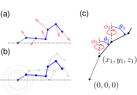
Figure 1: The origin of force by a constrained chain. A freely jointed chain (blue balls and sticks) is terminally pinned to a point (crosshair) and can move in full space or half space (dashed horizontal line). (a) Constraint (centrifugal) force. When freely jointed mass points of the chain move with some velocities (red arrows), the pin point will experience a force. The mass points can also exert force on the pin point when they recoil from the wall. (b) Thermodynamic (entropic) force. If the chain is pinned through a longer tether, more conformations become available. For example, the first mass point can explore a larger surface (compare blue and gray circles). Some conformations prohibited by the wall boundary can become acceptable as well when the tether is lengthened. This increase in conformational space leads to an increase in entropy, and thus a net force away from the surface. (c) Generalized coordinates in the global frame. The first three mass points of the chain are shown as black balls. The first three Cartesian coordinates $(x_{1},y_{1},z_{1})$ define the position of the first mass point with respect to the origin. The tether length is $r_{1}$. The positions of the rest are defined by global zenith ($\theta$) and azimuthal ($\phi$) angles.

In this study, we obtain the equilibrium force distribution due to a flexible polymer pinned in space or to a surface (Fig. 1). The key idea of our approach is to make random moves in the phase space of generalized position coordinates and their conjugate momenta and calculate microscopic forces exerted by the system. This approach is different from conventional Markov chain Monte Carlo methods that typically apply moves only in the position space. Because of the universality of entropic force, we expect our method to be applicable to a wide range of dynamic systems.

II Methods

II.1 Entropic force prediction

The entropic force can be found from a thermodynamic calculation

$$F=\frac{\partial A}{\partial r}=-k_{B}T\frac{\partial\log Q}{\partial r}$$ (1)

where $A$ is the free energy, $Q$ is the partition function, and $r$ is the generalized coordinate of interest. By measuring the change in the partition function as the chain is slightly displaced from the pin point, we can compute the entropic force. As shown in Fig. 1(b), when the tether is lengthened, additional conformations become available. For the full space case, the number of additional conformations is simply proportional to the area available to the first mass point. For the half-space case, we count the fraction of chain conformations compatible with the boundary condition Waters and Kim (2013), and calculate the small increase ($\Delta Q$) upon varying $r_{1}$ by $\Delta r_{1}$ to numerically approximate Eq. 1.

II.2 Phase space sampling

II.2.1 Monte Carlo sampling

Beginning from some initial conformation and initial generalized momenta, we can generate a set of conformations for a coarse-grained chain in a heat bath. The Hamiltonian of the chain in terms of generalized positions ($\mathbf{q}$) and momenta ($\mathbf{p}$) will be given by

$$H(\mathbf{q},\mathbf{p})=U(\mathbf{q})+\frac{1}{2}\mathbf{p}^{\mathsf{T}}\mathbf{M}^{-1}\mathbf{p}$$ (2)

where the first term $U$ is a potential energy based on chain deformation, and the second term is the kinetic energy expressed with the mass metric $\mathbf{M}$. For a freely jointed chain (FJC), $U$ is zero. We use the FJC model in this study because we want to obtain forces purely entropic of origin, but not due to physical interactions. The FJC model effectively coarse-grains an arbitrary polymer into Kuhn-length segments. The mass metric can be found from the Jacobian

$$(\mathbf{M})_{ij}=m(\mathbf{J}^{\mathsf{T}}\mathbf{J})_{ij}=m\frac{\partial x_{k}}{\partial q_{i}}\frac{\partial x_{k}}{\partial q_{j}}$$ (3)

$\mathbf{M}$ depends on $\mathbf{q}$ in non-Cartesian space. We choose $\theta$ and $\phi$ angles of each link measured in the global reference frame as the generalized coordinates (Fig. 1(c)). These are chosen over internal coordinates, as a change to the orientation of one link in the global frame will only affect two columns of the Jacobian matrix.

At each step, one of the momentum coordinates can be perturbed, and the new kinetic energy computed. The trial step can be accepted or rejected according to the Metropolis criterion on the total energy. The position coordinates can also be perturbed, which will require computing the change in kinetic energy (via a change in $\mathbf{M}(\mathbf{q})$) before the move can be accepted or rejected.

II.2.2 Equilibrium sampling

For longer chains, we sample points in the phase space using modal velocity decomposition Jain et al. . The key idea is that microstates specified by both $\mathbf{q}$ and $\mathbf{p}$ can be directly sampled from the probability density function ($\rho(\mathbf{q},\mathbf{p})$) to build the distribution of any microscopic variable. Our method is different from methods categorized as equilibrium sampling Zuckerman (2011) in that we sample both positions and momenta. For a canonical ensemble, $\rho(\mathbf{q},\mathbf{p})$ is given by

$$\rho(\mathbf{q},\mathbf{p})d^{2N}qd^{2N}p\propto e^{-\frac{\beta}{2}\dot{\mathbf{q}}^{\mathsf{T}}\mathbf{M(\mathbf{q})}\dot{\mathbf{q}}}d^{2N}qd^{2N}p,$$ (4)

where $\beta=1/k_{B}T$. In this form, sampling individual variables $q_{i}$ and $\dot{q}_{i}$ is not straightforward because they are coupled through $\mathbf{M(\mathbf{q})}$. Matrix diagonalization can be used to separate variables, but is not computationally efficient. Instead, the Cholesky decomposition can be used to express the symmetric, positive mass metric as

$$\mathbf{M}=m\bm{\mu}\bm{\mu}^{\mathsf{T}}$$ (5)

where $\mathbf{\mu}$ is a lower triangular matrix. By defining modal velocities as $\mathbf{v}=\bm{\mu}^{\mathsf{T}}\dot{\mathbf{q}}$, we can express the probability in a more separable form

$$\rho(\mathbf{q},\mathbf{p})d^{2N}qd^{2N}p\propto\sqrt{\text{det}(\mathbf{M(\mathbf{q})})}d^{2N}q\cdot e^{-\frac{\beta}{2}\mathbf{v}^{\mathsf{T}}\mathbf{v}}d^{2N}v$$ (6)

In this form, modal velocities ($v_{i}$) can be sampled independently of each other from a Gaussian distribution. However, positions ($q_{i}$) become coupled through $\text{det}(\mathbf{M(\mathbf{q})})$, which is known as the Fixman correction Fixman (1974). Hence, we adopt a hybrid approach where we first sample a microstate using normally distributed modal velocities and weight the microstate-dependent variable by the Fixman term. Calculating the determinant of the dense metric tensor is computationally intensive, however Fixman demonstrated that this is equivalent to the determinant of a smaller, tri-diagonal metric of the constrained coordinates (for details, see Supplemental Information).

II.3 Computing constraint force from positions and momenta

We consider a flexible chain terminally pinned in space or to a surface. We can use Lagrangian dynamics to calculate the constraint force as a function of positions and velocities of the $N$ mass points. Because distances between all adjacent mass points are constant, there are $2N+1$ degrees of freedom. We use three Cartesian coordinates $(x_{1},y_{1},z_{1})$ for the first mass point, and $2(N-1)$ angles ($\theta$ and $\phi$) for all other mass points of the chain (Fig. 1 (c)). Choosing generalized coordinates this way simplifies subsequent calculations. The Lagrangian is given by

$$L=\frac{1}{2}\dot{\mathbf{q}}^{\mathsf{T}}\mathbf{M}\dot{\mathbf{q}}$$ (7)

For the first mass point of the chain to be radially constrained at distance $r$, we introduce a Lagrange multiplier $\lambda$

$$L^{\prime}=\frac{1}{2}\dot{\mathbf{q}}^{\mathsf{T}}\mathbf{M}\dot{\mathbf{q}}+\lambda(r_{1}-r)$$ (8)

where $r_{1}=\sqrt{x_{1}^{2}+y_{1}^{2}+z_{1}^{2}}$. Using $L^{\prime}$ in the Euler-Lagrange equation with respect to $q_{k=1,2,3}$

$$\frac{d}{dt}\left(M_{ki}\dot{q}_{i}\right)=\frac{1}{2}\frac{\partial M_{ij}}{\partial q_{k}}\dot{q}_{i}\dot{q}_{j}+\lambda\frac{\partial r_{1}}{\partial q_{k}}$$ (9)

The first term on the right hand side vanishes as $\mathbf{M}$ does not depend on the Cartesian coordinates of the first mass point. Carrying out the differentiation on the left hand side produces an expression

$$M_{ki}\ddot{q}_{i}+\frac{\partial M_{ki}}{\partial q_{j}}\dot{q}_{i}\dot{q}_{j}=\lambda\frac{q_{k}}{r_{1}}$$ (10)

The second derivative of these terms must be solved for using the equation of motion for the angular coordinates.

$$M_{ij}\ddot{q}_{j}+\frac{\partial M_{ij}}{\partial q_{k}}\dot{q}_{j}\dot{q}_{k}=\frac{1}{2}\frac{\partial M_{jk}}{\partial q_{i}}\dot{q}_{j}\dot{q}_{k}$$ (11)

Solving for $\ddot{q}_{j}$ gives us

$$\ddot{q}_{j}=M_{ij}^{-1}\left(-\dot{q}_{l}\dot{q}_{k}\frac{\partial M_{il}}{\partial q_{k}}+\frac{1}{2}\dot{q}_{l}\dot{q}_{k}\frac{\partial M_{lk}}{\partial q_{i}}\right)$$ (12)

We can express this more concisely as the geodesic equation using the Christoffel connection coefficient, and making use of the symmetry in the first term under exchange of $l$ and $k$

$$\ddot{q}_{j}=-\dot{q}_{l}\dot{q}_{k}\Gamma_{lk}^{j}$$ (13)

where

$$\Gamma^{i}_{jk}=\frac{1}{2}M_{il}^{-1}\left(\frac{\partial M_{jl}}{\partial q_{k}}+\frac{\partial M_{kl}}{\partial q_{j}}-\frac{\partial M_{jk}}{\partial q_{l}}\right)$$ (14)

Substituting this back in produces the Cartesian components of the constraint force

$$\lambda\frac{q_{k}}{r_{1}}=\dot{q}_{i}\dot{q}_{j}\left(\frac{\partial M_{ik}}{\partial q_{j}}-\Gamma^{l}_{ij}M_{lk}\right)=\dot{q}_{i}\dot{q}_{j}\nabla_{i}M_{jk}$$ (15)

where $\nabla_{i}$ is the covariant derivative in the constrained subspace.

III Results

III.1 A single point constraint in space

We first considerd a thermally equilibrated flexible chain with one end pinned to a single point in full three dimensional space. By using the FJC model without a potential term, we can focus solely on entropic contributions to the force. We used the Monte Carlo phase space sampling method to build a canonical ensemble of chains. As shown in Fig. 2(a), kinetic energy is not equally partitioned between the mass points of the chain due to the constraints. The mass point nearest to the pin point has $\sim 25$% less kinetic energy whereas the endmost mass point has $\sim 25$% more. Most mass points in the middle have $k_{B}T$ on average, which would be expected for two degrees of freedom. Using these chain conformations and momenta, we calculated individual constraint forces from Lagrangian mechanics (Eq. 15). The distribution of constraint forces is highly asymmetric, including both positive and negative values with a sharp cusp. The mean constraint force is a negative pulling force, and does not depend on the chain length. Due to high skewness of the distribution, the mean force ($\sim 2k_{B}T/a$) is larger in magnitude than the most probable force ($\sim 1k_{B}T/a$). The standard deviation also has little dependence on the chain length (Fig. 2(d)).

We compared this mean constraint force with the entropic force ($F$) predicted by statistical mechanics. To seek more conformations, i.e., to increase entropy, the chain would prefer detachment from the pin point. As a result, the chain exerts a radial entropic force on the pin point. If the distance ($r$) between the pin point and the first mass point increases by $\Delta r$, the number of conformations will increase in proportion to the spherical surface spanned by the mass point. Therefore, the partition function ($Q$) is proportional to $4\pi r^{2}$, and the force at monomer distance $a$ is given by Eq. 1

$$F\approx\frac{k_{B}T}{Q}\frac{Q(a+\Delta r)-Q(a)}{\Delta r}=\frac{2k_{B}T}{a}$$ (16)

This entropic force is identical to the mean constraint force in magnitude, and is also independent of chain length as shown in Fig. 2(c).

Interestingly, the mean constraint force due to the entire chain is equal to the mean centrifugal force exerted by a single mass point. A radially constrained mass point has only two degrees of freedom, and therefore, according to the equipartition theorem, its mean kinetic energy is equal to $k_{B}T$. The mean of the centrifugal force ($f_{c}$) is

$$\langle f_{c}\rangle=\left\langle\frac{mv^{2}}{a}\right\rangle=\frac{2k_{B}T}{a}$$ (17)

Since the energy ($E=mv^{2}/2$) of a canonical ensemble is Boltzmann-distributed, the centrifugal force is exponentially distributed.

$$p(E)dE=e^{-\beta E}dE=\frac{a}{2}e^{-\beta af_{c}/2}df_{c}$$ (18)

As shown in Fig. 2(b), this exponential distribution (dashed line) can explain much of the distribution of negative constraint forces. However, positive forces and a significant fraction of large negative forces deviate from this distribution. This result suggests that freely jointed mass points beyond the nearest one can have a collective impact on the pin point.

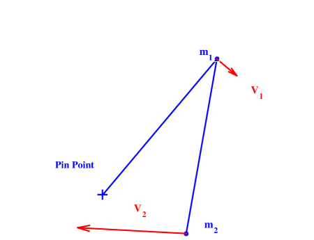
Figure 3: Origin of compressive forces. Some fraction of conformations (blue) and velocities (red) produce compressive forces along the first link in the chain, in contrast to the expectation from a single link acting as a pendulum. These occur when the chain is sharply bent, and the downstream mass points are moving more rapidly than those closer to the pin point ($v_{2}>v_{1}$).

To understand combined force generation by freely jointed mass points, we examined conformations that produce anomalous force values outside the range attributable to a single monomer. As shown in Fig. 3, instances where the force has the positive sign result from sharp bending and large velocities. For the simple case of a trimer in two dimensions, we can derive a condition for compressive force

$$\dot{\theta}_{2}^{2}\cos(\theta_{2}-\theta_{1})>2\dot{\theta}_{1}^{2}$$ (19)

This corresponds to the case where the centrifugal force exerted by $m_{2}$ on $m_{1}$ towards the pin point is more than twice that exerted by $m_{1}$ on the pin point in the opposite direction.

III.2 A single point constraint on a plane

We next considered a flexible chain attached to a surface. This confinement geometry arises in biology problems Petrov et al. (2013); Ludington et al. (2015) and polymer applications Milchev et al. (2010). The phase space sampling method applies the same way except that we only accept chain conformations that do not cross the boundary. We computed constraint forces at different chain lengths. As shown in Fig. 4(a) and (d), the distribution of constraint forces is highly asymmetric, similar to the full space case. Most forces are exerted in the outward direction, but a significant fraction of forces are compressive. The mean constraint force increases slightly as a function of chain length up to ten monomer lengths, but quickly reaches a constant value. The mean constraint force plateaus at about $2.5k_{B}T/a$, which is $25\text{\,}\mathrm{\char 37\relax}$ higher than the full space case.

For longer chains ($N>50$), phase space sampling becomes computationally expensive. We therefore adopted an equilibrium sampling method to calculate constraint forces. This method requires weighting by the Fixman correction. We computed a raw force distribution (uncorrected, ‘$\times$’ in Fig. 4), and later applied this correction (‘$\circ$’ in Fig. 4). Applying the Fixman correction lowers the average value of the force, as the largest forces are correlated with the largest extensions, which have a low weighting factor. This equilibrium method after correction produces similar distributions to the Monte Carlo method, highly asymmetric with more frequent negative than positive forces.

To compute the corresponding entropic force, we consider the increase in the accepted chain conformations upon increasing the distance to the first mass point. The partition function can then be numerically differentiated using Eq. 16 to obtain the entropic force. The result did not depend on the size of displacement chosen. As shown by the red dashed line in Fig. 4(b) and (e), the entropic forces based on conformational space only are slightly larger than the mean constraint forces ($2.6k_{B}T/a$ vs. $2.5k_{B}T/a$).

IV Discussion

We computed constraint forces exerted on a FJC in full space or half space by classical and statistical mechanical methods. Statistical mechanics was used to describe thermal fluctuations of the chain microstate, and classical mechanics was used to calculate the force required to constrain the chain against these thermal fluctuations. We found that the mean of constraint forces is equal to the entropic force calculated from the spatial derivative of the free energy. However, because constraint forces are asymmetrically distributed, the mean force is not equal to the most probable force. The force distribution is largely independent of the chain length beyond ten monomer lengths.

In this study, we treat the FJC as a canonical ensemble, which exchanges heat with the environment at a constant temperature. Our equilibration of microstates in the phase space is similar to the Andersen thermostat Andersen (1980) used in molecular dynamics with the added capability of simultaneously satisfying geometric constraints. At any instant, the mass points of the chain move with certain velocities at certain positions under the constraints set by the FJC model and the boundary. At a different time point, the mass points will adopt a different conformation with a different set of velocities as a result from collisions with the surrounding molecules of the heat bath. For each set of positions and momenta reset as a result of heat exchange, we calculate the microscopic constraint force.

The most nontrivial result from this study is that the force distribution is not Gaussian even in the long chain limit. Because the mass points are constrained in the freely jointed chain model, their impact on the tether are neither identical nor independent. As a result, the constraint force does not obey the central limit theorem. Consequently, the most probable value and the average value of force do not coincide with each other. Therefore, the entropic force that we derive from statistical mechanics might not be the most relevant quantity in all circumstances.

The fluctuation or second cumulant of an extensive thermodynamic variable can be easily calculated from the partition function when its conjugate intensive variable is fixed Marconi et al. (2008). Textbook examples are energy fluctuation in a canonical ensemble and particle number fluctuation in a grand canonical ensemble. On the other hand, the fluctuation of an intensive variable such as force cannot be derived from the partition function when the conjugate extensive variable is fixed, i.e. in a fixed-distance ensemble Rudoi and Sukhanov (2000); Gerland et al. (2001). Here, we use the FJC terminally constrained in full space to illustrate this point.

The constrained partition function ($Q_{c}$) is given by (See Supplemental Information.)

$$Q_{c}(r) =\int e^{-\beta H_{c}(\mathbf{q},\mathbf{p})}d^{2N}qd^{2N}p$$ (20a)

$$=\int e^{-\frac{\beta}{2}\mathbf{p}^{\mathsf{T}}\mathbf{M}^{-1}\mathbf{p}}d^{2N}qd^{2N}p,$$ (20b)

where $H_{c}$ is the Hamiltonian of the constrained chain. The mass metric $\mathbf{M}$ is a $2N\times 2N$ matrix that depends on $2N$ global angles $\mathbf{q}$. The dependence of the partition function on the distance between the end and the pin point ($r$) is explicity shown. Entropic force ($F$) arises because the constrained partition function increases with $r$, which is reflected by the thermodynamic relation:

$$F =\frac{1}{\beta}\frac{\partial\log Q_{c}(r)}{\partial r}$$ (21a)

$$=\int\frac{1}{\beta}\frac{\partial e^{-\beta H_{c}(\mathbf{q},\mathbf{p})}}{\partial r}d^{2N}qd^{2N}p/Q_{c}(r)$$ (21b)

$$=-\int\frac{\partial H_{c}(\mathbf{q},\mathbf{p})}{\partial r}\frac{e^{-\beta H_{c}(\mathbf{q},\mathbf{p})}}{Q_{c}(r)}d^{2N}qd^{2N}p$$ (21c)

$$=-\left\langle\frac{\partial H_{c}(\mathbf{q},\mathbf{p})}{\partial r}\right\rangle_{c}.$$ (21d)

The quantity in the constrained ensemble average can be identified with a microscopic force, which we denote as $f$. The second moment of $f$ can be shown to be

$$\left\langle\Delta f^{2}\right\rangle_{c}=\frac{1}{\beta^{2}}\frac{\partial^{2}\log Q_{c}(r)}{\partial r^{2}}+\left\langle\frac{\partial^{2}H_{c}}{\partial r^{2}}\right\rangle_{c}$$ (22)

Whereas the first term can be calculated from the constrained partition function, the second term depends on the microstate of the system. If the rigid constraint is relaxed to a spring, the second term is simply the stiffness ($\kappa$) of the spring. In this case, force fluctuations can be easily calculated, similar to those for a particle trapped in a harmonic potential Manosas and Ritort (2005); Mehraeen and Spakowitz (2012). However, the force fluctuation diverges in the stiff limit ($\kappa\rightarrow\infty$) Gerland et al. (2003). Therefore, to obtain force fluctuations with a hard constraint, one has to resort to computational means.

We showed that for a terminally pinned chain in full space, our phase space sampling method produces constraint forces whose mean is equal to the entropic force $2k_{B}T/a$. Using Eq. 20b, the entropic force can be worked out analytically. Integrating out the momentum dependence of $Q_{c}(r)$, one obtains

$$Q_{c}(r)=\text{const}\times\int\sqrt{\text{det}(\mathbf{M})}d^{2N}q$$ (23)

$Q_{c}(r)$ depends on $r$ through the mass metric $\mathbf{M}$. It can be shown that $\sqrt{\text{det}(\mathbf{M})}\propto r^{2}$ (Supplemental Information), and therefore the entropic force is given by

$$F=-\frac{2k_{B}T}{r}.$$ (24)

In comparison, the entropic force due to the pinned chain in a half space is difficult to derive because the limits of integration imposed by the half plane depend on $\mathbf{q}$ in some complex fashion.

People have used the method of images to calculate a simpler partition function in conformational space only Zhao et al. (2011); Hammer and Kantor (2014),

$$Q(h)\propto\int_{\text{half space}}d^{2N}q\propto\text{erf}\left(h\sqrt{\frac{3}{2Na^{2}}}\right)$$ (25)

where $h$ is the height of the pin point from the surface. By taking the derivative of $\log Q(h)$ with respect to $h$, a vertical entropic force can be derived. This vertical force increases with chain length for short chains, but is nearly constant at $k_{B}T/h$ for long chains. This force, however, is expected to be different from the mean constraint force obtained from our phase sampling methods for several reasons. First, the method of images yields only the vertical component of the entropic force out of mathematical convenience. Second, the analytical expression (Eq. 25) is correct only in the Gaussian limit of long chains. Third, the conformational partition function in Eq. 25 does not include the kinetic effect. However, it is unclear if removing the kinetic effect would significantly alter the mean force prediction. Therefore, we numerically computed the conformational partition function as a function of $r$ instead of $h$, and obtained a thermodynamic force conjugate to $r$ using Eq. 16. This force is only slightly larger than the entropic force obtained by phase space sampling as shown in Fig. 4(b) and (e).

As the chain length becomes longer, the Monte Carlo method becomes computationally expensive. A faster method is to sample conformations directly from an a priori distribution. For example, to simulate a canonical ensemble of ideal gas, one can randomly sample velocities from the Maxwell-Boltzmann distribution and assign them to randomly positioned particles. Such equilibrium sampling, however, is not straightforward for a constrained system due to the coupling of $\mathbf{p}$ through $\mathbf{M}$. By decomposing $\mathbf{M}$, we can obtain modal velocities that individually obey a Gaussian distribution. Such a transformation skews the distribution by the Fixman term, which must be corrected for to unbiasedly sample the phase space. Our results show that this correction is warranted (Fig. 4(e) and (f)).

Both phase space sampling methods we introduce in this work are based on theoretically correct interpretations of the constrained partition function. The Monte Carlo phase space sampling method has the advantage of not requiring the Fixman correction to produce the correct average force prediciton. Additionally, this method may prove more useful for geometries such as polymer chains with a constant end-to-end distance. In such cases, selecting conformations that fit a given distribution is difficult but perturbing a conformation that already lies within that distribution is comparatively easy. The chief disadvantage of this method is the computational time required to perturb the chain, and the large number of steps required to adequately explore the conformational space.

In contrast, the equilibrium phase space sampling, where uncorrelated conformations are selected, and momenta assigned after, is much quicker for free chains. This lack of correlation may more easily lend this method to large-scale parallelization as well. One minor disadvantage of this method is that it introduces a discrepancy in the mean force, unless the sampled conformations are weighted by the Fixman correction.

V Conclusions

We introduced two different computational methods to sample microstates of a freely jointed chain in an unbiased manner. Unlike mainstream Monte Carlo methods that explore the conformational space only, our methods explore the complete phase space to obtain full distribution of any velocity-dependent microscopic variable in thermal equilibrium. We applied these methods to a terminally pinned chain in full space and half space to calculate constraint forces. The force distribution was non-Gaussian and asymmetric with both tensile and compressive forces. Most notably, the most likely force was smaller in magnitude than the mean force, which is more commonly considered both theoretically and experimentally. The constraint force exhibited little chain-length dependence beyond $\sim 10$ monomer lengths. The presence of a plane leads to a larger mean constraint force. This work can be extended to investigate fluctuating forces using more realistic polymer models and confinement.

VI Acknowledgement

The authors acknowledge financial support from Georgia Institute of Technology and the Burroughs Wellcome Fund Career Award at the Scientific Interface. We thank Tung Le, Jiyoun Jeong, and the rest of the Kim lab for careful reading of the manuscript. We also thank Dr. Kurt Wiesenfeld and Dr. Toan Nguyen for helpful discussions.

Figure 2: Chain pinned in full space. (a) Distribution of kinetic energy at different points along the chain. The first mass point after the pinning position has less energy than average, and the last one has slightly more. The mean kinetic energy remains $Nk_{B}T$ in all cases. Shown are results from different chain lengths ($N$=10, 20, and 30). (b) Distribution of radial constraint forces. While the mean constraint force equals that due to a single mass point, additional links in the polymer chain increase likelihood of strong pulling forces and even introduce the possibility of compressive forces. The most probable force is near $-1$ shown by the vertical dotted line. Distributions are computed for different chain lengths ($N$=2, 9, and 29) from 150 K samples. (c) Mean constraint force and entropic force. The average force (black circles) is independent of length, and matches the predicted entropic force (red line), which results from the first mass point confined to the surface of a sphere moving to a larger radius. (d) Standard deviation of constraint forces. The standard deviation is on the same order of magnitude as the mean force, and quickly saturates as chain length increases.

Figure 4: Chain pinned to plane. (a) Distribution of forces for phase-space sampled chains. The surface effect shifts the mean of the distribution slighty, but the shape is not changed relative to the free case. The most probable force is near $-1$ shown by the vertical dotted line. Distributions are computed for different chain lengths ($N$=2, 9, and 29), from 150 K samples. (b) Mean force from chains sampled via phase space Monte Carlo (circles) and thermodynamic force from conformation space partition function (dashed line). The average force lies above the $2/a\beta$ value of the free chain case, as additional entropy is gained by pulling away from the surface. The mean force exhbits some length dependence not seen in the free chain case, however it quickly saturates around 10 links in the polymer chain. (c) Standard deviation of sampled forces. As in the free chain case, the deviation is on the same order of magnitude as the mean force. It grows slightly as a function of length, quickly saturating around 5-7 links. (d) Distribution of forces for conformational space sampled chains. The same distribution observed in (a) persists as we consider longer chains ($N$=2, 9, and 99). The most probable force is near $-1$ shown by the vertical dotted line. The curves in the figure represent 300 K samples. (e) Mean force from equilibrium sampled chains, before applying the Fixman correction ($\times$) and after ($\circ$), displayed along side the partition function prediction (dashed line). The mean force remains constant as we explore larger lengths than were accessible in (b). (f) Standard deviation for force from equilibrium sampled chains, with ($\circ$) and without ($\times$) the Fixman correction.

Supplemental Information

VI.1 Dependence of the mass metric on the end constraint

The Cartesian coordinates of the n-th mass point are given by ($n\geq 2$).

$$x_{n} =x_{1}+\sum_{i=2}^{N}\sin\theta_{i}\cos\phi_{i}$$

$$y_{n} =y_{1}+\sum_{i=2}^{N}\sin\theta_{i}\sin\phi_{i}$$

$$z_{n} =z_{1}+\sum_{i=2}^{N}\cos\theta_{i}.$$

It is assumed that all adjacent mass points are joined by an inextensible linker of unit length. The spherical coordinates of the first mass point are given by

$$x_{1} =r_{1}\sin\theta_{1}\cos\phi_{1}$$

$$y_{1} =r_{1}\sin\theta_{1}\sin\phi_{1}$$

$$z_{1} =r_{1}\cos\theta_{1}.$$

We define two sets of generalized coordinates $\mathbf{u}=\{r_{1},\theta_{i},\phi_{i}\}$ and a subset of unconstrained coordinates $\mathbf{q}=\{\theta_{i},\phi_{i}\}$ where $i=1,2,...,N$. The Jacobian matrix $\mathbf{J}$ with respect to $\mathbf{u}$ can be constructed from smaller Jacobians for individual mass points. The Jacobian matrix is a $3\times 3$ matrix for the first mass point:

$$\mathbf{J}_{1}=\begin{bmatrix}\dfrac{\partial x_{1}}{\partial r_{1}}&\dfrac{\partial x_{1}}{\partial\theta_{1}}&\dfrac{\partial x_{1}}{\partial\phi_{1}}\\[10.00002pt] \dfrac{\partial y_{1}}{\partial r_{1}}&\dfrac{\partial y_{1}}{\partial\theta_{1}}&\dfrac{\partial y_{1}}{\partial\phi_{1}}\\[10.00002pt] \dfrac{\partial z_{1}}{\partial r_{1}}&\dfrac{\partial z_{1}}{\partial\theta_{1}}&\dfrac{\partial z_{1}}{\partial\phi_{1}}\end{bmatrix}=\begin{bmatrix}\sin\theta_{1}\cos\phi_{1}&r_{1}\cos\theta_{1}\cos\phi_{1}&-r_{1}\sin\theta_{1}\sin\phi_{1}\\ \sin\theta_{1}\sin\phi_{1}&r_{1}\cos\theta_{1}\sin\phi_{1}&r_{1}\sin\theta_{1}\cos\phi_{1}\\ \cos\theta_{1}&-r_{1}\sin\theta_{1}&0\end{bmatrix},$$

and a $3\times 2$ matrix for the rest:

$$\mathbf{J}_{i\geq 2}=\begin{bmatrix}\dfrac{\partial x_{i}}{\partial\theta_{i}}&\dfrac{\partial x_{i}}{\partial\phi_{i}}\\[10.00002pt] \dfrac{\partial y_{i}}{\partial\theta_{i}}&\dfrac{\partial y_{i}}{\partial\phi_{i}}\\[10.00002pt] \dfrac{\partial z_{i}}{\partial\theta_{i}}&\dfrac{\partial z_{i}}{\partial\phi_{i}}\end{bmatrix}=\begin{bmatrix}\cos\theta_{i}\cos\phi_{i}&-\sin\theta_{i}\sin\phi_{i}\\ \cos\theta_{i}\sin\phi_{i}&\sin\theta_{i}\cos\phi_{i}\\ \sin\theta_{i}&0\end{bmatrix}.$$

The total Jacobian can be expressed as a block matrix:

$$\mathbf{J}=\begin{bmatrix}\mathbf{J}_{1}&0&\cdots&0\\ \mathbf{J}_{1}&\mathbf{J}_{2}&\cdots&0\\ \vdots&\vdots&\ddots&\vdots\\ \mathbf{J}_{1}&\mathbf{J}_{2}&\cdots&\mathbf{J}_{N}\end{bmatrix}.$$

The mass matric becomes a $(2N+1)\times(2N+1)$ square matrix:

$$\mathbf{M}_{u}=m\mathbf{J}^{\mathsf{T}}\mathbf{J}=m\begin{bmatrix}N\mathbf{J}_{1}^{\mathsf{T}}\mathbf{J}_{1}&(N-1)\mathbf{J}_{1}^{\mathsf{T}}\mathbf{J}_{2}&\cdots&\mathbf{J}_{1}^{\mathsf{T}}\mathbf{J}_{N}\\ (N-1)\mathbf{J}_{2}^{\mathsf{T}}\mathbf{J}_{1}&(N-1)\mathbf{J}_{2}^{\mathsf{T}}\mathbf{J}_{2}&\cdots&\mathbf{J}_{2}^{\mathsf{T}}\mathbf{J}_{N}\\ \vdots&\vdots&\ddots&\vdots\\ \mathbf{J}_{N}^{\mathsf{T}}\mathbf{J}_{1}&\mathbf{J}_{N}^{\mathsf{T}}\mathbf{J}_{2}&\cdots&\mathbf{J}_{N}^{\mathsf{T}}\mathbf{J}_{N}\end{bmatrix},$$

where $r_{1}$-dependence is completely isolated in the first block row and column. Expanding the block matrices, one can obtain $r_{1}$-dependence of the matrix elements:

$$\mathbf{M}_{u}=m\begin{bmatrix}N&0&0&...\\ 0&Nr_{1}^{2}&0&\propto r_{1}&\cdots&\propto r_{1}\\ 0&0&Nr_{1}^{2}\sin^{2}\theta_{1}&\propto r_{1}&\cdots&\propto r_{1}\\ \vdots&\propto r_{1}&\propto r_{1}&\ddots\\ &\vdots&\vdots\\ &\propto r_{1}&\propto r_{1}&\end{bmatrix},$$

where $\propto r_{1}$ denotes terms proportional to $r_{1}$. We can obtain a $2N\times 2N$ submatrix $\mathbf{M}_{q}$ by excluding the first row and column of $\mathbf{M}_{u}$:

$$\mathbf{M}_{q}=m\begin{bmatrix}Nr_{1}^{2}&0&\propto r_{1}&\cdots&\propto r_{1}\\ 0&Nr_{1}^{2}\sin^{2}\theta_{1}&\propto r_{1}&\cdots&\propto r_{1}\\ \propto r_{1}&\propto r_{1}&\ddots\\ \vdots&\vdots\\ \propto r_{1}&\propto r_{1}&\end{bmatrix}.$$ (S1)

It is straightforward to show $\text{det}(\mathbf{M}_{q})\propto r_{1}^{4}$, which gives rise to an entropic force $2k_{B}T/r$ upon constraining $r_{1}=r$. To demonstrate this, we transform the partition function for the unconstrained system to the constrained one den Otter (2013). We use the Hamiltonian of a freely jointed chain without the end constraint to express the partition function:

$$Q_{u}=\int e^{-\frac{\beta}{2}\mathbf{p}_{u}^{\mathsf{T}}\mathbf{M}_{u}^{-1}\mathbf{p}_{u}}d^{2N+1}ud^{2N+1}p_{u}.$$

$\mathbf{p}_{u}$ is a vector of $2N+1$ momenta conjugate to $\mathbf{u}$. Delta functions are introduced to apply the end constraint on $r_{1}$:

$$Q_{c}(r)=\int e^{-\frac{\beta}{2}\mathbf{p}_{u}^{\mathsf{T}}\mathbf{M}_{u}^{-1}\mathbf{p}_{u}}\delta(r_{1}-r)\delta(\dot{r}_{1})d^{2N+1}ud^{2N+1}p_{u},$$

where $r$-dependence of the constrained partition function is explicitly shown. The delta functions can be handled by decomposing the mass metric and using the transformation rule $d^{2N+1}p_{u}=d^{2N}p_{q}(Nmd\dot{r_{1}})$

$$Q_{c}(r) =\int e^{-\frac{\beta}{2}\mathbf{p}_{q}^{\mathsf{T}}\mathbf{M}_{q}^{-1}\mathbf{p}_{q}}e^{-\frac{\beta}{2}m\dot{r}_{1}^{2}}\delta(r_{1}-r)\delta(\dot{r}_{1})dr_{1}(Nmd\dot{r}_{1})d^{2N}qd^{2N}p_{q}$$

$$=Nm\int e^{-\frac{\beta}{2}\mathbf{p}_{q}^{\mathsf{T}}\mathbf{M}_{q}^{-1}(r)\mathbf{p}_{q}}d^{2N}qd^{2N}p_{q}.$$

Integrating with $\mathbf{p}_{q}$, we can obtain the $r$-dependence of the partition function:

$$Q_{c}(r)\propto\int\sqrt{\text{det}(\mathbf{M}_{q}(r))}d^{2N}q$$ (S2)

VI.2 Calculation of the metric determinant

Chain conformations acquired from equilibirum sampling of the conformational space, without consideration of momentum space, will require a weighting factor given by the determinant of the metric tensor in the constrained space. The metric in the constrained space is generally dense, and so calculating the determinant $g^{\alpha}$ is computationally intensive. Fixman Fixman (1974) made use of the simple form of the metric determinant $g$ in the unconstrained space, to find the desired $g^{\alpha}$ from the determinant $g^{\beta}$ in the smaller, orthogonal subspace spanned by the constrained dimensions.

$$g=g^{\alpha}g^{\beta}\rightarrow g^{\alpha}=g/g^{\beta}$$ (S3)

This is further simplified by considering the inverse $\mathbf{H}$ of the metric $\mathbf{G}^{\beta}$ for the orthogonal subspace of constrained dimensions. This has the form

$$H_{ij}=\sum_{k=0}^{N}\frac{\partial r_{i}}{\partial\mathbf{x}_{k}}\frac{\partial r_{j}}{\partial\mathbf{x}_{k}}$$ (S4)

where $r_{i}$ is the bond length between points $\mathbf{x}_{i-1}$ and $\mathbf{x}_{i}$. The terms in the sum are only non-zero when $i=j\pm 1$ and $k=i\mbox{ or }i-1$. This ultimately produces a tridiagonal matrix

$$\mathbf{H}=\begin{bmatrix}2&-\mathbf{\hat{r}}_{1}\cdot\mathbf{\hat{r}}_{2}&0&\cdots&0&0\\ -\mathbf{\hat{r}}_{1}\cdot\mathbf{\hat{r}}_{2}&2&-\mathbf{\hat{r}}_{2}\cdot\mathbf{\hat{r}}_{3}&\cdots&0&0\\ 0&-\mathbf{\hat{r}}_{2}\cdot\mathbf{\hat{r}}_{3}&2&\cdots&0&0\\ \vdots&\vdots&\vdots&\ddots&\vdots&\vdots\\ 0&0&0&\cdots&2&-\mathbf{\hat{r}}_{N-1}\cdot\mathbf{\hat{r}}_{N}\\ 0&0&0&\cdots&-\mathbf{\hat{r}}_{N-1}\cdot\mathbf{\hat{r}}_{N}&2\end{bmatrix}.$$ (S5)

Expanding this matrix in minors gives a recursive formula for the determinant $h$, where $\mathbf{\hat{r}}_{n}$ is the unit relative position vector pointing from (n-1)-th mass point to n-th mass point.

$$h_{n}=2h_{n-1}-(\mathbf{\hat{r}}_{n}\cdot\mathbf{\hat{r}}_{n-1})^{2}h_{n-2}$$ (S6)

For equal mass points, we begin with the base cases $h_{0}=h_{1}=1$. Note this is slightly different than the Fixman case ($h_{1}=2$) as we are also constraining the position of the first mass point. Once we have computed $h$, the determinant $g^{\alpha}$ is easily found from

$$g^{\alpha}=g\cdot h$$ (S7)

References

- Kardar and Golestanian (1999) M. Kardar and R. Golestanian, Reviews of Modern Physics 71, 1233 (1999).
- Leckband and Israelachvili (2001) D. Leckband and J. Israelachvili, Quarterly reviews of biophysics 34, 105 (2001).
- Jacobson (1995) T. Jacobson, Physical Review Letters 75, 1260 (1995).
- Verlinde (2011) E. Verlinde, Journal of High Energy Physics 2011, 1 (2011).
- Turner et al. (2002) S. Turner, M. Cabodi, and H. Craighead, Physical Review Letters 88, 128103 (2002).
- Prinsen et al. (2009) P. Prinsen, L. T. Fang, A. M. Yoffe, C. M. Knobler, and W. M. Gelbart, The Journal of Physical Chemistry B 113, 3873 (2009).
- Zhao et al. (2011) S.-L. Zhao, J. Wu, D. Gao, and J. Wu, The Journal of chemical physics 134, 065103 (2011).
- Guo et al. (2005) K. Guo, F. Qiu, H. Zhang, and Y. Yang, The Journal of chemical physics 123, 074906 (2005).
- Odenheimer et al. (2005) J. Odenheimer, D. W. Heermann, and M. Brill, International Journal of Modern Physics C 16, 1561 (2005).
- Bickel et al. (2001) T. Bickel, C. Jeppesen, and C. Marques, The European Physical Journal E 4, 33 (2001).
- Bartolo et al. (2002) D. Bartolo, A. Ajdari, J.-B. Fournier, and R. Golestanian, Physical review letters 89, 230601 (2002).
- Jeppesen et al. (2001) C. Jeppesen, J. Y. Wong, T. L. Kuhl, J. N. Israelachvili, N. Mullah, S. Zalipsky, and C. M. Marques, Science 293, 465 (2001).
- Guo et al. (2011) Z. Guo, M. Gibson, S. Sitha, S. Chu, and U. Mohanty, Proceedings of the National Academy of Sciences 108, 3947 (2011).
- Koslover and Spakowitz (2012) E. F. Koslover and A. J. Spakowitz, Physical Review E 86, 011906 (2012).
- Waters and Kim (2013) J. T. Waters and H. D. Kim, Macromolecules 46, 6659 (2013).
- (16) A. Jain, I.-H. Park, and N. Vaidehi, Journal of chemical theory and computation 8, 2581.
- Zuckerman (2011) D. M. Zuckerman, Annual Review of Biophysics 40, 41 (2011).
- Fixman (1974) M. Fixman, Proceedings of the National Academy of Sciences 71, 3050 (1974).
- Petrov et al. (2013) A. S. Petrov, S. S. Douglas, and S. C. Harvey, Journal of Physics: Condensed Matter 25, 115101 (2013).
- Ludington et al. (2015) W. B. Ludington, H. Ishikawa, Y. V. Serebrenik, A. Ritter, R. A. Hernandez-Lopez, J. Gunzenhauser, E. Kannegaard, and W. F. Marshall, Biophysical journal 108, 1361 (2015).
- Milchev et al. (2010) A. Milchev, L. Klushin, A. Skvortsov, and K. Binder, Macromolecules 43, 6877 (2010).
- Andersen (1980) H. C. Andersen, The Journal of chemical physics 72, 2384 (1980).
- Marconi et al. (2008) U. M. B. Marconi, A. Puglisi, L. Rondoni, and A. Vulpiani, Physics reports 461, 111 (2008).
- Rudoi and Sukhanov (2000) Y. G. Rudoi and A. D. Sukhanov, Physics-Uspekhi 43, 1169 (2000).
- Gerland et al. (2001) U. Gerland, R. Bundschuh, and T. Hwa, Biophysical Journal 81, 1324 (2001).
- Manosas and Ritort (2005) M. Manosas and F. Ritort, Biophysical journal 88, 3224 (2005).
- Mehraeen and Spakowitz (2012) S. Mehraeen and A. J. Spakowitz, Physical Review E 86, 021902 (2012).
- Gerland et al. (2003) U. Gerland, R. Bundschuh, and T. Hwa, Biophysical journal 84, 2831 (2003).
- Hammer and Kantor (2014) Y. Hammer and Y. Kantor, Physical Review E 89, 022601 (2014).
- den Otter (2013) W. K. den Otter, Journal of chemical theory and computation 9, 3861 (2013).