Optimal Training for Non-Feedback Adaptive Modulation over Rayleigh Fading Channels

Abstract

Time-varying fading channels present a major challenge in the design of wireless communication systems. Adaptive schemes are often employed to adapt the transmission parameters to receiver-based estimates of the quality of the channel. We consider a pilot-based adaptive modulation scheme without the use of a feedback link. In this scheme, pilot tones (known by sender and receiver) are periodically sent through the channel for the purpose of channel estimation and coherent demodulation of data symbols at the receiver. We optimize the duration and power allocation of these pilot symbols to maximize the information-theoretic achievable rates using binary signaling. We analyze four transmission policies and numerically show how optimal training in terms of duration and power allocation varies with the channel conditions and from one transmission policy to another. We prove that for a causal estimation scheme with flexible power allocation, placing all the available power on one pilot is optimal.

I Introduction

In digital mobile communications, fast fading degrades the Bit Error Rate (BER) of the channel and inhibits coherent detection. It is known that performance is limited by channel estimation errors [1, 2, 3, 4]. Pilot Symbol Assisted Modulation (PSAM) is a technique that has been introduced in [5] to mitigate these effects. In this scheme, known training symbols (pilots) are periodically inserted into the data frame for the purpose of channel estimation and coherent demodulation of the data symbols.

Furthermore, channel-adaptive modulation dynamically adjusts certain transmission parameters such as the constellation size, transmitted power, and code rate according to the channel quality. Adaptive signaling provides in general higher bit rates (relative to conventional nonadaptive methods) by increasing the transmission throughput under favorable channel conditions and reducing it as the channel condition is degraded.

Some of the previous adaptive schemes rely on a channel-feedback link to provide the transmitter with the Channel Side Information (CSI) [6, 7]. In [8], the authors consider employment of adaptive modulation with one pilot in addition to delayed feedback to the transmitter and prove that power adaptation via periodic feedback can increase the achievable rates. Similarly, in [9], authors consider pilot-based adaptive modulation where estimate is fed back to transmitter in order to adapt data and pilot power and study the optimal policy for power allocation for data and pilot symbols. Authors in [10] discuss adaptive modulation with feedback and develop an adaptive scheme that accounts for both channel estimation and prediction errors in order to meet a target Bit Error Rate (BER). In [11], the authors attempt to optimize the spectral efficiency subject to a specific BER constraint in a pilot-based adaptive modulation setup with feedback. The above mentioned works study the performance of such systems and prove adaptive modulation using pilots can increase the achievable rates in general. However, systems that rely on a channel-feedback link present some disadvantages because of the modeling complexity on one hand and its infeasibility on the other hand when the channel is fading faster than it can be estimated (or predicted) and fed back to the sender. Optimizing the pilot placement, power allocation and modulation schemes in a pilot-based setup is an active area of research, whether in the case of a single receiver [8, 9, 12, 13, 14, 15, 16, 17, 10] or multiple receivers [17, 18, 19].

A modified pilot-based adaptive modulation scheme over Rayleigh fading channels was presented in [20]. This scheme adapts the coded modulation strategy at the sender to the quality of the channel estimation (estimation error variance) at the receiver without requiring any channel feedback. In this work we study the performance of this non-feedback adaptive modulation scheme over time-varying Rayleigh fading channels. Unlike the scheme in [20], we consecutively send a cluster of $k$ pilots ($k\geq 1$) per data frame with $k$ being an optimization variable [21]. We determine the optimal duration and power allocation of the training period under different transmission policies for both causal and non-causal estimation. We study such systems at low Signal-to-Noise-Ratio (SNR) (we consider the received SNR) levels and the performance is measured in terms of achievable rates using binary signaling. We prove that the “optimal” power allocation scheme which minimizes the error variance of the estimates of the channel parameters –which is set up offline without requiring feedback– in case of causal estimation is the one in which all the available power is allocated on one pilot, if constraints allow it.

The organization of this paper is as follows. In Section II, we present the fading channel model, the adaptive transmission technique we use to transmit over the channel as well as the receiver details. The measure of performance is discussed in Section III, the optimal power allocation for causal estimation is proved in Section IV and the numerical results are presented in Section V. In Section VI, we present possible extensions to other fading models and Section VII concludes the paper.

II Preliminaries

II-A The Channel Model

Consider the single-user discrete-time model for the Rayleigh fading channel,

$$Y_{i}=R_{i}X_{i}+N_{i},$$

where $i$ is the time index, $X_{i}\in\mathbb{C}$ is the channel input at time $i$, $Y_{i}\in\mathbb{C}$ is its output, and $R_{i}$ and $N_{i}$ are independent complex circular Gaussians random variables with zero mean and variance $\sigma_{R}^{2}$ and $\sigma_{N}^{2}$ respectively. The amplitude of the fading coefficient $R_{i}$ is then Rayleigh distributed and its phase is uniform over $[-\pi,\,\pi)$. To account for power constraints, the input is subject to

$$\textsf{E}\left[{\left|X_{i}\right|^{2}}\right]\leq P_{i},$$

for some parameters $\{P_{i}\}$ –that could be all equal to a constant for example. Since from an information theoretic perspective scaling the output by $1/\sigma_{R}$ does not change the mutual information, we assume without loss of generality that $\sigma_{R}=1$. The variance of the noise $\sigma_{N}^{2}$ is to be generally interpreted as $(\sigma_{N}^{2}/\sigma_{R}^{2})$.

We assume in this study that the fading process follows a stationary first-order Gauss-Markov model introduced in [22], i.e.,

$$R_{i}=\alpha R_{i-1}+Z_{i},$$ (1)

where the samples $\{Z_{i}\}$ are Independent and Identically-Distributed (IID) complex circular Gaussians with mean zero and variance equal to $\sigma_{Z}^{2}=\left(1-\alpha^{2}\right)$ such that $\alpha\in\left[0,1\right)$ to guarantee stationarity.

Even though we analyze the benefits of pilot clustering by assuming that the autocorrelation function of the fading process is derived from a stationary first-order Gauss-Markov model (1), we argue in Section VI that the methodology may be readily adapted to other models and present the case of a Jakes’ model [23] that takes into account higher orders of correlation.

II-B The Adaptive Transmission Scheme

At regular intervals, the transmitter successively sends $k$ known pilot symbols whose purpose is to enable the estimation of the channel at the receiver. The channel estimation is solely based on the pilot symbols and no data-directed estimation is used. For each time sample $i$, the receiver computes the Minimum Mean-Square Estimate (MMSE) of the channel, the quality of which –measured through the estimate error variance– depends on its position with respect to the pilot symbols. After estimation, the channel, as seen by the receiver, is a Rician channel whose specular part is given by the estimate and whose Rayleigh component is given by the zero-mean Gaussian-distributed estimation error.

Although the scheme is adaptive, it does not use feedback to determine its policy. The key idea is that the transmitter adapts to the quality of channel estimation (specifically to the mean-square error which is independent of the value of the estimate available only at the receiver) rather than the estimate of the channel. Since the estimation error variance is computed offline, the adaptive transmission scheme can then be determined offline as well and adopted by the transmitter. Even though three is no feedback to the transmitter, it is aware of the statistics of the estimation error beforehand.

The transmitter employs multiple codebooks in an interleaved fashion as shown in Figure 1. It adapts its throughput to the estimation error variance by coding the data symbols according to their distance from the training pilots. Symbols that are far away from the pilots encounter poorer channel estimates at the receiver and are therefore coded with lower rate codes, while closer symbols benefit from small estimation error variance and are coded with higher rate codes.

Figure 1: Multiple Codebook Interleaving

We only consider binary signaling. The motivation for this choice is multiple folds. First, in [24] the authors prove that for discrete-time memoryless Rayleigh fading channels subject to average power constraints, the capacity achieving distribution is discrete with a finite number of mass points. Moreover, a binary distribution was found to be optimal at low and moderate values of SNR [24, 25, 26]. Second, for a memoryless Rician fading channel, Luo [27] established a similar result that, combined with Gallager’s in [25], implies that the binary input distribution is asymptotically optimal at low SNR [27]. Consequently, we choose the alphabet of every codebook to consist in general of two symbols:

$$\left\{\begin{array}[]{llll}m_{1}&=a_{1}+jb_{1}&\text{\small with probability}&p_{1}\\ m_{2}&=a_{2}+jb_{2}&\text{\small with probability}&p_{2}=(1-p_{1}).\end{array}\right.$$

The rate of the codebooks is adjusted by modifying the probability distribution of the mass points. Numerical results in [20, 12] indicate that the optimal mass points always lie between the extremes of on-off keying (optimal for the IID Rayleigh fading case where no CSI is available at the receiver) and the antipodal signaling (optimal for a perfectly known channel). It is worth noting that some of the work in the literature consider these two extremes for designing the constellation mapping and try to optimize the transmission model in the case of imperfect CSI based on the SNR level [12]. Moreover, any rotational transformation of the two mass points will not affect the mutual information [24, 27]. Therefore an optimal input distribution consists of two mass points $m_{1},m_{2}\in\mathbb{R^{*}}$ with $-\sqrt{P}\leq m_{1}<0$ and $m_{2}\geq\sqrt{P}$.

II-C Channel Estimation at the Receiver

Given a pilot spacing interval $T$, we send $k$ pilots in the beginning of every data frame as shown in Figure 2. When transmitting a pilot at time index $i$, the input of the channel is $\sqrt{P_{i}}$ and its output is,

$$Y_{i}=\sqrt{P_{i}}R_{i}+N_{i},\qquad i=0,\cdots,k-1.$$

Figure 2: Pilot Symbols and Channel Estimation

On the receiver side, we perform MMSE estimation based on the received signal during training. More precisely, we denote by $\mathcal{S}$ the set of indices corresponding to the received pilots $\{Y_{s}\}_{s\in\mathcal{S}}$ involved in estimating $R_{j}$ for $j=k,\ldots,T-1$. Therefore, when $\mathcal{S}=\left\{0,\ldots,k-1\right\}$ we say we are performing causal MMSE estimation, and when $\mathcal{S}=\left\{0,\ldots,k-1,\,T,\ldots,T+k-1\right\}$ the MMSE estimate is said to be non-causal.

Next, we compute the MMSE estimate $\hat{R}_{j}\left(\left\{Y_{s}\right\}_{s\in\mathcal{S}}\right)$ of $R_{j}$ for $j=k,\ldots,T-1$. Since the random variables $\left\{R_{j},\,\,\{Y_{s}\}_{s\in\mathcal{S}}\right\}$ are jointly Gaussian, the MMSE estimator is linear and is identical to the Linear Least-Square Estimator (LLSE) the error variance $v_{j}$ of which is,

$${\displaystyle v_{j}=1-\Lambda_{R_{j},\,\{Y_{s}\}_{s\in\mathcal{S}}}\;\Lambda_{\{Y_{s}\}_{s\in\mathcal{S}}}^{-1}\;\Lambda_{R_{j},\,\{Y_{s}\}_{s\in\mathcal{S}}}^{T}\,\,,}$$ (2)

where $\Lambda_{R_{j},\,\{Y_{s}\}_{s\in\mathcal{S}}}$ is the cross-covariance matrix between $R_{j}$ and $\{Y_{s}\}_{s\in\mathcal{S}}$ and $\Lambda_{\{Y_{s}\}_{s\in\mathcal{S}}}$ is the autocovariance of the vector of received pilots $\{Y_{s}\}_{s\in\mathcal{S}}$.

We note that the estimation error variance in equation (2) may be computed offline at design time –and therefore no feedback is needed to the encoder– and is only dependent on the autocorrelation function of $\{R_{j}\}$, the transmitted pilots and the noise spectral density.

III Achievable Rates

We consider the transmission scheme shown in Figure 2 with symbols sent with power $P_{j}$ for $j=0,\ldots,T-1$. Given a sample $\left\{y_{s}\right\}_{s\in\mathcal{S}}$, the received symbols can be written

$$Y_{i}=R_{i}X_{i}+N_{i}=\left(\hat{R}_{i}+\Gamma_{i}\right)X_{i}+N_{i},\quad\text{for }i=k,\ldots,T-1,$$

where $\Gamma_{i}$ is a zero-mean complex Gaussian error term that has a variance $v_{i}$. Therefore,

$$p\left(y_{i}|x_{i},\left\{y_{s}\right\}_{s\in\mathcal{S}}\right) = \mathcal{N}_{\mathbb{C}}\left(\hat{R}_{i}x_{i},\,v_{i}\left|x_{i}\right|^{2}+\sigma_{N}^{2}\right)=\frac{1}{\pi\left(v_{i}\left|x_{i}\right|^{2}+\sigma_{N}^{2}\right)}e^{-\frac{\left|y_{i}-\hat{R}_{i}x_{i}\right|^{2}}{v_{i}\left|x_{i}\right|^{2}+\sigma_{N}^{2}}}.$$

When ignoring the fading correlation from one transmitted frame to another, the mutual information per symbol due to interleaving can be written as

$$\frac{1}{T}\,I\left(\;\{X_{i}\}_{i=0}^{T-1}\;;\;\{Y_{i}\}_{i=0}^{T-1}\;|\;\{Y_{s}\}_{s\in\mathcal{S}}\;\right)=\textsf{E}_{\{Y_{s}\}_{s\in\mathcal{S}}}\left[{\frac{1}{T}\sum_{i=k}^{T-1}I\left(X_{i};Y_{i}|\{y_{s}\}_{s\in\mathcal{S}}\right)}\right]\\ =\frac{1}{T}\sum_{i=k}^{T-1}\textsf{E}_{\hat{R}_{i}}\left[{I\left(X_{i};Y_{i}|\hat{R}_{i}\right)}\right],$$ (3)

where the expectation is now over the random variable $\hat{R}_{i}$. Note that $\hat{R}_{i}$ is a linear combination of the observations

$$\hat{R}_{i}=\sum_{m\in\mathcal{S}}\beta_{m}Y_{m}=R_{i}-\Gamma_{i}\sim\mathcal{N}_{\mathbb{C}}(0,1-v_{i}).$$ (4)

III-A The Computation Method

The $i^{th}$ term, $\textsf{E}_{\hat{R}_{i}}\left[{I\left(X_{i};Y_{i}|\hat{R}_{i}\right)}\right]$, in equation (3) depends on the choice of the corresponding binary probability distribution fully characterized by the three parameters $\{m_{1},m_{2},p_{1}\}_{i}$. This distribution (for $i=k,\ldots,T-1$) determines the rate of the corresponding codebook and should be chosen to maximize the mutual information quantity in (3). Therefore, we are interested in solving

$$\frac{1}{T}\sum_{i=k}^{T-1}\max_{\{m_{1},\,m_{2},\,p\}_{i}}\textsf{E}_{\hat{R}_{i}}\left[{I\left(X_{i};Y_{i}|\hat{R}_{i}\right)}\right],$$ (5)

subject to $\textsf{E}\left[{|X_{i}|^{2}}\right]\leq P_{i}$ for all $i=k,\ldots,T-1$.

Furthermore, examining the probability law (4) of $\hat{R}_{i}$ indicates that the elementary quantity $\displaystyle{\max_{\{m_{1},\,m_{2},\,p\}_{i}}\textsf{E}_{\hat{R}_{i}}\left[{I\left(X_{i};Y_{i}|\hat{R}_{i}\right)}\right]}$ in (5) is only a function of the estimation error variance $v_{i}$ and power $P_{i}$ of the symbol. We define

$$I_{sub}(P_{i},\,\,v_{i})=\max_{\{m_{1},\,m_{2},\,p\}_{i}}\textsf{E}_{\hat{R}_{i}}\left[{I\left(X_{i};Y_{i}|\hat{R}_{i}\right)}\right],$$

where the maximization is subject to $\textsf{E}\left[{|X_{i}|^{2}}\right]\leq P_{i}$ and $\hat{R_{i}}\sim\mathcal{N}_{\mathbb{C}}(0,1-v_{i})$. Thereafter the achievable rates become

$$\frac{1}{T}\,I\left(\;\{X_{i}\}_{i=0}^{T-1}\;;\;\{Y_{i}\}_{i=0}^{T-1}\;|\;\{Y_{s}\}_{s\in\mathcal{S}}\;\right)=\frac{1}{T}\sum_{i=k}^{T-1}I_{sub}(P_{i},\,\,v_{i}).$$ (6)

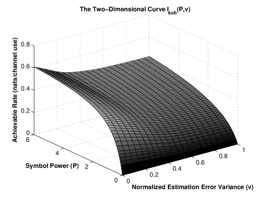
The two dimensional curve $I_{sub}(P,\,\,v)$ is computed over a fine grid $\mathscr{V}=\{0\leq P\leq P_{max},0\leq v\leq 1\}$ as shown in Figure 3. Then given a transmission strategy consisting of an inter-pilot spacing $T$, $k$-pilot clustering, and a power allocation $P_{j}$ for $j=0,\ldots,T-1$, we calculate using equation (2) the estimation error variance $v_{j}$ for $j=k,\,\dots,T-1$. The corresponding elementary mutual information quantity $I_{sub}(P_{j},\,v_{j})$ can now be interpolated from the data set $\{\mathscr{V},\,I_{sub}(P,\,v)\}$ and used to compute the normalized sum in (6).

Figure 3: The two-dimensional curve $I_{sub}(P,\,\,v)$

Finally, note that the error variance is a function of the power of the pilots $\{P_{s}\}_{s\in\mathcal{S}}$. Hence equation (6) can also be written as

$$I\left(\;\{X_{i}\}_{i=k}^{T-1}\;;\;\{Y_{i}\}_{i=k}^{T-1}\;|\;\{Y_{s}\}_{s\in\mathcal{S}}\;\right)=\frac{1}{T}\sum_{i=k}^{T-1}I_{sub}\left(P_{i},\,\,\{P_{s}\}_{s\in\mathcal{S}}\right).$$ (7)

III-B The transmission policy

We consider four types of transmission policies and we study how the optimal training strategy differs from one policy to another, analytically in Section IV and numerically in Section V.

III-B1 Policy I

The pilot symbols and the data symbols are transmitted with the same amount of power, i.e.,

$$P_{s}=P,\quad\forall s=0,\ldots,k-1\qquad\&\qquad P_{i}=P,\quad\forall\,i=k,\ldots,T-1.$$

Therefore. for a given channel model, $k$-pilot training, and an inter-pilot spacing $T$, the achievable rate in equation (7) is a function of $P$ only.

III-B2 Policy II

In this policy, a flat power allocation is adopted for both the pilot symbols and the data symbols, but we allow the two levels to be different. More precisely,

$$P_{s}=P_{tr}\quad\forall s=0,\ldots,k-1\qquad\&\qquad P_{i}=P_{d},\quad\forall\,i=k,\ldots,T-1.$$

The achievable rate is a function of $P_{tr}$ & $P_{d}$ which satisfy

$$\frac{1}{T}\sum_{j=0}^{T-1}P_{j}=\frac{1}{T}\bigl{[}kP_{tr}+(T-k)P_{d}\bigr{]}\leq P.$$

III-B3 Policy III

Following a flat power allocation for pilots ($P_{s}=P_{tr},\forall s=0,\ldots,k-1$), the data symbols are sent with power $P_{i}$ for $i=k,\ldots,T-1$. These power levels satisfy

$$\frac{1}{T}\sum_{j=0}^{T-1}P_{j}=\frac{1}{T}\left[kP_{tr}+\sum_{j=k}^{T-1}P_{j}\right]\leq P.$$

III-B4 Policy IV

We send both the pilots and data symbols with variable power $P_{j}$ for $j=0,\ldots,T-1$. The constraint on the power levels is now given by

$$\frac{1}{T}\sum_{j=0}^{T-1}P_{j}\leq P.$$

IV Optimal Power Allocation for Causal Estimation

In this section we find the optimal power allocation and training duration for policies II, III and IV under causal estimation. These optimal solutions are found by applying the result of Theorem 1 stated hereafter. The theorem implies that if we let $kP_{tr}$ be the total power “budget” for the training period, everything else being equal, among all the training power allocation schemes $\{P_{s}\}_{s=0}^{k-1}$ such that

$$\sum_{s=0}^{k-1}P_{s}=kP_{tr},$$ (8)

the optimal one is the one where all the power is allocated to the last time slot $(k-1)$.

For causal MMSE estimation $\mathcal{S}=\{0,\cdots,k-1\}$ and equation (2) can be written as

$$v_{j} =1-\Lambda_{R_{j},\,\{Y_{s}\}_{s\in\mathcal{S}}}\;\Lambda_{\{Y_{s}\}_{s\in\mathcal{S}}}^{-1}\;\Lambda_{R_{j},\,\{Y_{s}\}_{s\in\mathcal{S}}}^{T}\qquad\qquad\qquad j=k,\cdots,(T-1)$$

$$=1-\alpha^{2(j-k+1)}\left(\alpha^{k-1}\,\,\alpha^{k-2}\,\,\cdots\,\,1\right)\;D^{T}\;\left[D\;A\;D^{T}+\sigma_{N}^{2}\;I\right]^{-1}\;D\;\left(\begin{array}[]{c}\alpha^{k-1}\\ \vdots\\ 1\end{array}\right),$$ (12)

where $A$ is the $k\times k$ symmetric, positive definite autocovariance matrix of the channel fading coefficients $\{R_{s}\}_{s\in\mathcal{S}}$, and $D$ is the $k\times k$ “input” matrix:

$$A=\begin{pmatrix}1&\alpha&\cdots&\alpha^{k-1}\\ \alpha&1&\cdots&\alpha^{k-2}\\ \vdots&\vdots&\ddots&\vdots\\ \alpha^{k-1}&\alpha^{k-2}&\cdots&1\end{pmatrix},\qquad D=\begin{pmatrix}\sqrt{P_{0}}&0&\cdots&0\\ 0&\sqrt{P_{1}}&\cdots&0\\ \vdots&\vdots&\ddots&\vdots\\ 0&0&\cdots&\sqrt{P_{k-1}}\end{pmatrix}.$$

A power allocation that minimizes the error variances of the estimates for all $\{j\}$’s –subject to the power constraint (8)– is naturally an optimal one. Examining (12), we note that a power allocation that minimizes $v_{j_{o}}$ for some $j_{o}$ will also minimize $v_{j}$ for all $\{j\}$’s, as it will be one that maximizes

$$\left(\alpha^{k-1}\,\,\alpha^{k-2}\,\,\cdots\,\,1\right)\;D^{T}\;\left[D\;A\;D^{T}+\sigma_{N}^{2}\;I\right]^{-1}\;D\;\left(\begin{array}[]{c}\alpha^{k-1}\\ \vdots\\ 1\end{array}\right).$$ (13)

The power allocation that maximizes (13) is the subject of the following theorem, proven in Appendix A.

Theorem 1.

The expression (13) is maximized when all the available power is allocated to the last pilot, i.e., $P_{j}=0$, for all $0\leq j\leq(k-2)$ and $P_{k-1}=kP_{tr}$.

We note that Theorem 1 holds whenever one allows the power allocation during the training period to vary across the pilots. We also note that the result holds irrespective of how the power is allocated for the data.

Implications on the training duration

• When considering policy IV, the powers of the individual training symbols are allowed to vary and the theorem states that all the power should be allocated to the last training symbol. Factoring in the loss of achievable rates due to training, it becomes clear that the optimal duration is that of one pilot transmission.

• Since the achievable rates using policy III are less or equal to those of policy IV, and since the optimal solution for policy IV is that of a “flat” power allocation over the duration of the training –which is one, then the solution is also optimal for policy III.

• Finally, since the statement of the theorem is valid irrespective of how the power is allocated during data transmission and specifically even when a flat power allocation is used, the result implies that for policy II, using a training duration of one pilot is optimal as well.

Naturally, these statements are true if the power level during training is optimized. In Section V we validate numerically these results.

V Numerical Results

For a given channel model, a given SNR (power constraints), and estimation technique (causal or non-causal), we numerically determine the optimal training strategy consisting of:

1. The duration of training or the number of pilots $k$.

2. The inter-pilot spacing $T$.

3. The power allocation for the pilots and data symbols in a transmitted frame, according to the transmission policy used.

In our work, the quality measure is the achievable rates which we compute for pilot clustering/training period of up to six pilots in each frame. We study the low received SNR regime (SNR values of -3dB, 0dB, 3dB, and 6dB) for a first-order Gauss-Markov fading process with values of $\alpha=0.9,0.95,0.97,\,\textrm{and}\,0.99$. On the receiver side, causal and non-causal estimation are investigated. We present hereafter graphs for some chosen test cases and compare the rates achieved using 1, 2, 3, 4, 5, and 6-pilot clustering strategies for different scenarios of SNR and fading correlation levels.

We note first that the numerical results confirm the observation previously made that the achievable rate in equation (3) depends on the choice of $\{m_{1},m_{2},p_{1}\}_{i}$, i.e., the input distribution of the $i$-th symbol. As the symbol gets further away from the training pilots, the channel estimation quality (measured through the estimate error variance) is degraded and hence the amount of information sent over the channel decreases. This is translated by shifting $\{m_{1},m_{2},p_{1}\}_{i}$ from the antipodal distribution (optimal for a perfectly known channel) with $p_{1}\approx p_{2}$ (high entropy) toward the other extreme of on-off keying (optimal for the IID Rayleigh fading case) with $p_{1}\gg p_{2}$ (low entropy).

We also note that in the case of causal estimation, our numerical results are consistent with the results in Section IV.

V-A Results for Transmission Policy I

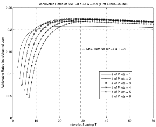
For transmission policy I, pilot clustering proves to achieve higher rates under certain conditions compared to the 1-pilot scheme. In Figure 4, for an SNR = 0dB, $\alpha$ = 0.99 and causal estimation, training with 4 pilots and inter-pilot spacing of $T$=29 symbols is optimal. A percent increase of 8.2% in information rate is achieved relative to the best rate achievable with a 1-pilot scheme. The results for other test cases are shown in Table I.

Figure 4: Achievable Rates for policy I, for SNR = 0dB and $\alpha$ = 0.99 with Causal Estimation.

TABLE I: Achievable Rates for Different Transmission Policies

Test Case	Policy I	Policy II	Policy III	Policy IV
$\alpha\,=\,0.9$	nP=4	nP=1	nP=1	nP=1
SNR = 0dB	T=29	T=22	T=23	T=22
Causal Estimation	Rate$\approx$0.2247	Rate$\approx$0.2418	Rate$\approx$0.2422	Rate$\approx$0.2422
	8.2%$\uparrow$1	7.6%$\uparrow$2
$\alpha\,=\,0.97$	nP=1	nP=1	nP=1	nP=1
SNR = 6dB	T=15	T=15	T=15	T=15
Causal Estimation	Rate$\approx$0.3782	Rate$\approx$0.3829	Rate$\approx$0.3836	Rate$\approx$0.3836
		1.2%$\uparrow$2
$\alpha\,=\,0.97$	nP=3	nP=1	nP=1	nP=1
SNR = -3dB	T=19	T=18	T=18	T=18
Non-Causal Estimation	Rate$\approx$0.1374	Rate$\approx$0.1470	Rate$\approx$0.1472	Rate$\approx$0.1472
	4.3%$\uparrow$1	6.9%$\uparrow$2
Using Jakes’ model:
$f_{d}\,=\,100\,$Hz, $f_{s}\,=\,10\,$KHz	nP=2	nP=1	nP=1	nP=1
SNR = 3dB	T=14	T=13	T=13	T=13
Causal Estimation	Rate$\approx$0.3224	Rate$\approx$0.3508	Rate$\approx$0.3510	Rate$\approx$0.3510
	4%$\uparrow$1	8.8%$\uparrow$2
Using Jakes’ model:
$f_{d}\,=\,100\,$Hz, $f_{s}\,=\,10\,$KHz	nP=4	nP=1	nP=1	nP=1
SNR = 0dB	T=29	T=30	T=30	T=30
Non-Causal Estimation	Rate$\approx$0.2843	Rate$\approx$0.3064	Rate$\approx$0.3064	Rate$\approx$0.3064
	16%$\uparrow$1	7.7%$\uparrow$2

• relative to the rate achieved by the 1-pilot scheme (Policy I).

• relative to the achievable rate under Policy I.

However there are some scenarios when pilot-clustering is not useful. For the case when SNR = 6dB, $\alpha$ = 0.97 and causal estimation, the 1-pilot scheme presents optimal rates.

Moreover in Figure 5 at an SNR=0dB, and $\alpha$=0.9 with causal estimation, training is not beneficial in the first place because the information rate is less than that achieved over an IID Rayleigh fading channel.

Figure 5: Achievable Rates for policy I, for SNR = 0dB and $\alpha$ = 0.9 with Causal Estimation.

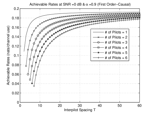
As a conclusion, we can distinguish three cases. The first is when training is not applicable. The second is when the 1-pilot scheme gives the highest rates. And finally the third when pilot clustering is beneficial. From our numerical results, we note that as SNR increases and coherence time decreases, clustering becomes useless and the whole scheme is pushed toward the 1-pilot training strategy and even to the extreme case of no training at all. This is directly related to the fact that training is inefficient (less CSI) when fading decorrelates quickly or when SNR is high.

V-B Results for Transmission Policy II

In this policy, the pilots are sent with fixed power $P_{tr}$ ( per pilot ) and so are the symbols that are transmitted with power $P_{d}$ (Section III-B2), such that $\displaystyle{\frac{1}{T}\sum_{j=0}^{T-1}P_{j}\leq P}$. Therefore, the optimal training strategy includes determining the optimal power allocation ($P_{tr}$ and $P_{d}$) for the transmitted frame. Here the notion of SNR is naturally associated with the average power $P$.

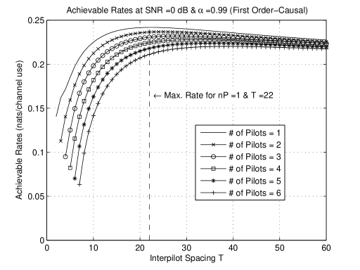
Figure 6 shows the achievable rates for SNR=0dB, and $\alpha$=0.99 with causal estimation. Unlike the results for policy I (Figure 4), training with 4 pilots is not optimal anymore. The 1-pilot scheme (with $T$=22) now offers 7.6% increase in the achievable rate compared to the 4-pilot scheme for policy I. The corresponding optimal power allocation across the transmission frame is shown in Figure 7.

Figure 6: Achievable Rates for policy II, for SNR = 0dB and $\alpha$ = 0.99 with Causal Estimation.

Figure 7: Optimal Symbol Power Allocation (one frame) for policy II, for SNR = 0dB and $\alpha$ = 0.99 with Causal Estimation.

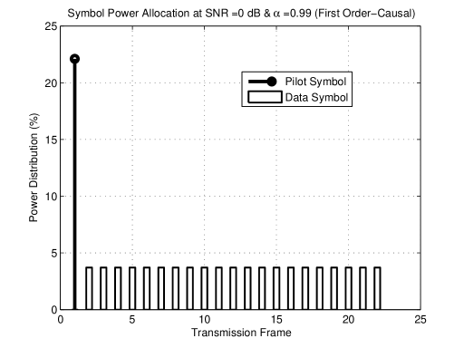
The rest of the results are presented in Table I and they all confirm that, as expected pilot clustering is not optimal for policy II, and for any transmission strategy where the pilots’ power is subject to optimization for that matter. In this case, the transmitter decreases the estimation error variance (higher throughput) by boosting the power of the single pilot instead of increasing the number of pilots $k$ and getting penalized by the normalizing term $\displaystyle{\frac{1}{T}}$ in equation (7).

If a peak power constraint is imposed on the power of the pilots, the optimal training duration will not necessarily be one pilot. This can be seen from Figure 8 which shows the optimal power allocation across the transmission frame for SNR=0dB, and $\alpha$=0.99 with causal estimation whenever a peak constraint $P_{tr}\leq 3P$ is imposed. This constraint is effectively imposing a maximum Peak-to-Average Power Ratio (PAPR) value of 3.

Figure 8: Optimal Symbol Power Allocation (one frame) for policy II, for SNR = 0dB and $\alpha$ = 0.99 with Causal Estimation and peak constraint $P_{tr}\leq 3P$.

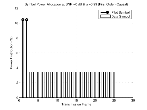
As mentioned earlier, there are some scenarios where training is not useful and the rate is always less than that achieved over an IID Rayleigh fading channel. This is observed with causal estimation for an SNR=0dB and $\alpha$=0.9 for example. In that case all the power is allocated to the data symbols indicating that training is not beneficial.

V-C Results for Transmission Policy III

For policy III, we send the data symbols with varying power as we hold on to a flat power allocation for the pilots. As already shown in the Section IV, clustering is not useful for this case as well. The transmitter boosts the power of the single pilot used in training to decrease the error variance and increase the achievable rate.

The numerical results are in accordance with those of Section IV and they show how the power of the symbols is adapted to the estimation error variance. In Figure 9, the power allocated to each symbol and the variation of the error variance are presented for an SNR=0dB, and $\alpha$=0.99 with non-causal estimation. This shows that symbols with lower variance are sent with higher power and vice versa. However we should note that power variations among the data symbols is not profound.

Figure 9: Optimal Symbol Power Allocation (one frame) for policy III, for SNR = 0dB and $\alpha$ = 0.99 with Non-Causal Estimation.

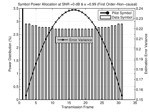
The achievable rates for other cases are summarized in Table I. It is noticed that adapting the symbol power to the quality of estimation introduces a slight increase in achievable rates compared to policy II. As a result, one can say that uniform power allocation for the data symbols is sufficiently close to optimal and presents a more practical transmission strategy.

V-D Results for Transmission Policy IV

Here both the pilots and data symbols are sent with varying power (Section III-B4). However from the results for transmission policy III, we already know that sending the data symbols with uniform power is very close to optimal.

Let us consider the case for an SNR=0dB, and $\alpha$=0.99. We choose a 4-pilot training scheme. For causal estimation, the power allocated to the pilots is shown in Figure 10. We notice that all of the power was found numerically to be allocated to the pilot closest to the symbols leaving the rest of the pilots that are further away with no power and therefore useless, which is consistent with the results of Theorem 1 and Section IV. Combining this result with the penalty factor $\displaystyle{\frac{1}{T}}$ in equation (3), we reach the conclusion that the 1-pilot scheme is always optimal (Table I).

Figure 10: Optimal Symbol Power Allocation (one frame) for policy IV, for SNR = 0dB and $\alpha$ = 0.99 with Causal Estimation.

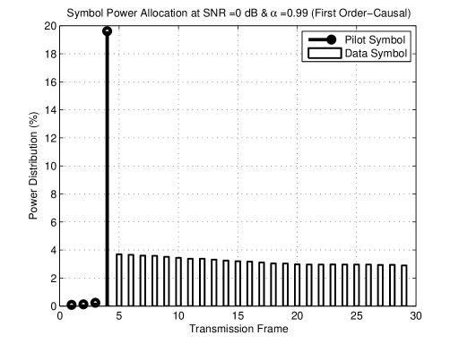
A similar result is shown in Figure 11 for the non-causal estimation scenario. The powers of the first pilot (playing a prominent role in the non-causal part) and last pilot (with a prominent role in the causal part) are increased.

Figure 11: Optimal Symbol Power Allocation (one frame) for policy IV, for SNR = 0dB and $\alpha$ = 0.99 with Non-Causal Estimation.

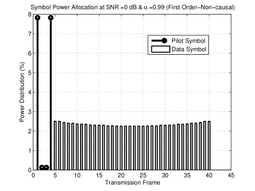
Whenever a peak power constraint is imposed on the power of the pilots, the optimal training duration will potentially involve pilot clustering. The optimal duration and power allocation in Figure 12 are for an SNR=0dB, and $\alpha$=0.99 with causal estimation whenever a peak constraint $P_{tr}\leq 3P$ is imposed.

Figure 12: Optimal Symbol Power Allocation (one frame) for policy IV, for SNR = 0dB and $\alpha$ = 0.99 with Causal Estimation and peak constraint $P_{tr}\leq 3P$.

VI Other Fading Process Models

Whenever the fading process follows a different model, appropriate results may be readily derived as the numerical optimization is only dependent on the autocovariance function of the process as seen from equation (2). In what follows, we present sample results using Jakes’ model.

Jakes’ Model

In Jakes’ model [23], the normalized (unit variance) continuous-time autocorrelation function of the fading process is given by

$$\phi_{RR}(\tau)=J_{0}(2\pi f_{d}\tau),$$

where $J_{0}(.)$ is the zeroth-order Bessel function of the first kind and $f_{d}$ is the maximum Doppler frequency. For the purposes of discrete-time simulation of this model [28], the autocorrelation sequence becomes

$$\phi_{RR}[l]=J_{0}(2\pi f_{d}\,T_{s}\,|l|),$$

where $1/T_{s}$ is the symbol rate.

In Table I we list a sample of the results obtained for a bandwidth $f_{s}=10$ kHz and a Doppler shift of $f_{d}=100$ Hz. For example, optimal training consists of $k=4$ and $T=29$ when we have an SNR=0dB and non-causal estimation. Throughput is improved by 16% in this case.

VII Conclusion

We studied the performance of the non-feedback pilot-based adaptive modulation scheme [20, 21, 29] over time-varying Rayleigh fading channels. We measured the performance in terms of achievable rates using binary signaling and we investigated the benefits of pilot clustering as well as power allocation.

We introduced a modular method to compute the rates in an efficient manner. Moreover, four types of transmission policies were analyzed. For each policy, we determined the optimal training strategy consisting of:

1. The duration of training.

2. The inter-pilot spacing.

3. The power allocation for the pilots and data symbols in the frame.

Pilot clustering proved to be useful in the low SNR–high coherence time range where training is efficient (Policy I). However, when the pilot power is subject to optimization (Policies II, III and IV), training for a smaller period but with boosted power becomes more beneficial than training with more pilots. We proved that the optimal training duration using causal estimation is indeed one whenever the power level during training is optimized and allowed to take arbitrary values. Numerical results suggest that this is also the case when using non-causal estimation at the receiver.

We also noted that the numerical computations indicate that a flat power allocation across the data slots in a frame is very close to optimal whenever the pilot power is subject to optimization.

On the other hand, training is useless in the high SNR–small coherence time range and the rate is always less than that achieved over an IID Rayleigh fading channel. Several test cases are shown throughout this work to analyze how optimal training varies with channel conditions and from one transmission policy to another.

Extensions to this work can include adaptive schemes that integrate temporal and spatial components like the Multiple-Input Multiple-Output (MIMO) scenario.

Appendix A

In this appendix we provide a proof for Theorem 1. For notational convenience, define

$$\phi \;\hat{=}\;V^{T}\;D^{T}\;\left[D\;A\;D^{T}+\sigma_{N}^{2}\;I\right]^{-1}\;D\;V,$$

where $V=\left(\alpha^{k-1}\,\,\alpha^{k-2}\,\,\cdots\,\,1\right)^{T}$, $A$ is the $k\times k$ symmetric, positive definite autocovariance matrix of the channel fading coefficients $\{R_{s}\}_{s\in\mathcal{S}}$, and $D$ is the $k\times k$ “input” matrix:

$$A=\begin{pmatrix}1&\alpha&\cdots&\alpha^{k-1}\\ \alpha&1&\cdots&\alpha^{k-2}\\ \vdots&\vdots&\ddots&\vdots\\ \alpha^{k-1}&\alpha^{k-2}&\cdots&1\end{pmatrix},\quad D=\begin{pmatrix}\sqrt{P_{0}}&0&\cdots&0\\ 0&\sqrt{P_{1}}&\cdots&0\\ \vdots&\vdots&\ddots&\vdots\\ 0&0&\cdots&\sqrt{P_{k-1}}\end{pmatrix},\quad V=\left(\begin{array}[]{c}\alpha^{k-1}\\ \alpha^{k-2}\\ \vdots\\ 1\end{array}\right).$$

Note that $\phi<1$ for any $k\geq 1$ because $\phi=1-v_{k-1}$. We establish first the following lemma:

Lemma 1.

Let $U$ be a $k\times k$ diagonal matrix with non-negative entries $\{x_{i}\}_{i=0}^{k-1}$ on the diagonal. Among all the permutations of the $\{x_{i}\}$’s, the one that maximizes $V^{T}\left[A+U\right]^{-1}V$ is one where the diagonal entries are in non-increasing order.

Proof.

Assume that $\{x_{i}\}_{i=0}^{k-1}$ are in the following order: $0\leq x_{0}\leq x_{1}\leq\cdots\leq x_{k-1}$. We prove in what follows that $U=diag(x_{k-1},x_{k-2},\cdots,x_{0})$ maximizes $V^{T}\left[A+U\right]^{-1}V$ using induction on $k$. To highlight the dependence on $k$ we denote $\varphi_{k}=V_{k}^{T}\left[A_{k}+U_{k}\right]^{-1}V_{k}$, which is a positive quantity due to the positive definiteness of $\left[A_{k}+U_{k}\right]^{-1}$.

Base Cases

For $k=1$, $\varphi_{1}=\frac{1}{1+x_{0}}$ and the statement holds. Examine now the case $k=2$:

$$U=diag(x_{0},x_{1}) \Longrightarrow\varphi_{2}=\frac{(\alpha^{2}x_{1}+x_{0}-\alpha^{2}+1)}{(x_{0}+1)(x_{1}+1)-\alpha^{2}}$$

$$U=diag(x_{1},x_{0}) \Longrightarrow\varphi_{2}=\frac{(\alpha^{2}x_{0}+x_{1}-\alpha^{2}+1)}{(x_{1}+1)(x_{0}+1)-\alpha^{2}}.$$

Since $\alpha<1$ and $x_{1}\geq x_{0}$, the second value is larger.

Induction Step

Suppose the property holds true up to $k-1$ ($k-1\geq 2$) and we prove in what follows that it holds true for $k$:

$$\varphi_{k}=\begin{pmatrix}\alpha^{k-1}&\alpha^{k-2}&\cdots&1\end{pmatrix}\;\left[A_{k}+U_{k}\right]^{-1}\;\begin{pmatrix}\alpha^{k-1}\\ \alpha^{k-2}\\ \vdots\\ 1\end{pmatrix},$$

where $A_{k}$ and $U_{k}$ are square matrices of size $k$. We prove that $\varphi_{k}$ is maximized when $\{x_{i}\}_{i=0}^{k-1}$ are placed in non-increasing order on the diagonal matrix $U_{k}$. The proof proceeds as follows: We first “fix” $x_{k-1}$ on the last diagonal entry of $U_{k}$ and prove that $\{x_{i}\}_{i=0}^{k-2}$ should be in a non-increasing order to maximize $\varphi_{k}$. Next, we “fix” $\{x_{i}\}_{i=0}^{k-3}$ on the first $(k-2)$ diagonal entries of $U_{k}$ and we prove that, if $x_{k-2}\leq x_{k-1}$, having $U=diag\{x_{0},x_{1},\cdots,x_{k-3},x_{k-1},x_{k-2}\}$ (versus $U=diag\{x_{0},x_{1},\cdots,x_{k-3},x_{k-2},x_{k-1}\}$) gives us a larger value of $\varphi_{k}$, completing the proof.

$\bullet$ Using a block form, we write $[A_{k}+U_{k}]$ as:

$$A_{k}+U_{k}=\begin{pmatrix}E&F\\ F^{T}&G\end{pmatrix},$$

where

$$E=\begin{pmatrix}x_{0}+1&\alpha&\cdots&\alpha^{k-2}\\ \alpha&x_{1}+1&\cdots&\alpha^{k-3}\\ \vdots&\vdots&\ddots&\vdots\\ \alpha^{k-2}&\alpha^{k-3}&\cdots&x_{k-2}+1\end{pmatrix},\quad F=\begin{pmatrix}\alpha^{k-1}\\ \alpha^{k-2}\\ \vdots\\ \alpha\end{pmatrix}=\alpha V_{k-1}\quad\&\quad G=\begin{pmatrix}x_{k-1}+1\end{pmatrix}.$$

This allows us to express $[A_{k}+U_{k}]^{-1}$ as [30]:

$$[A_{k}+U_{k}]^{-1}=\begin{pmatrix}E^{-1}+E^{-1}F[G-F^{T}E^{-1}F]^{-1}F^{T}E^{-1}&-E^{-1}F[G-F^{T}E^{-1}F]^{-1}\\ -[G-F^{T}E^{-1}F]^{-1}F^{T}E^{-1}&[G-F^{T}E^{-1}F]^{-1}\end{pmatrix}$$

and

$$\varphi_{k}=\, F^{T}\left[E^{-1}+E^{-1}F[G-F^{T}E^{-1}F]^{-1}F^{T}E^{-1}\right]F-[G-F^{T}E^{-1}F]^{-1}F^{T}E^{-1}F$$

$$-F^{T}E^{-1}F[G-F^{T}E^{-1}F]^{-1}+[G-F^{T}E^{-1}F]^{-1},$$

which reduces to:

$$\varphi_{k} =F^{T}E^{-1}F+\frac{\left(1-F^{T}E^{-1}F\right)^{2}}{\left[x_{k-1}+1-F^{T}E^{-1}F\right]}=F^{T}E^{-1}F+\frac{\left(x_{k-1}+1-F^{T}E^{-1}F-x_{k-1}\right)^{2}}{\left[x_{k-1}+1-F^{T}E^{-1}F\right]}$$

$$=\left(-x_{k-1}+1\right)+\frac{x_{k-1}^{2}}{\left[x_{k-1}+1-F^{T}E^{-1}F\right]}.$$

The scalar $F^{T}E^{-1}F$ is equal to $\alpha^{2}\varphi_{k-1}$. Indeed, $F$ is of size $(k-1)\times 1$ and equal to $\alpha V_{k-1}$, and $E$ is a $(k-1)\times(k-1)$ sub-matrix of the form $[A_{k-1}+U_{k-1}]$. Since $\alpha<1$, the scalar $F^{T}E^{-1}F$ is less than one and the denominator is a positive quantity. Therefore, with $x_{k-1}$ fixed, $\varphi_{k}$ is maximized when $F^{T}E^{-1}F$ is maximized. By the induction step, with a fixed $x_{k-1}$ the remaining $x_{i}$’s should be “placed” in decreasing order on the diagonal of $E$ –and $U$– to maximize $\varphi_{k}$.

$\bullet$ Now fix $\{x_{i}\}_{i=0}^{k-3}$. We prove that with $x_{k-2}\leq x_{k-1}$, $U=diag\{x_{0},x_{1},\cdots,x_{k-3},x_{k-1},x_{k-2}\}$ gives us a larger value for $\varphi_{k}$. To do this, we consider a different decomposition of the matrix $[A_{k}+U_{k}]$,

$$A_{k}+U_{k}=\begin{pmatrix}E&F\\ F^{T}&G\end{pmatrix}$$

where now

$$E=\begin{pmatrix}x_{0}+1&\alpha&\cdots&\alpha^{k-3}\\ \alpha&x_{1}+1&\cdots&\alpha^{k-4}\\ \vdots&\vdots&\ddots&\vdots\\ \alpha^{k-3}&\alpha^{k-4}&\cdots&x_{k-3}+1\end{pmatrix}\,F=\begin{pmatrix}\alpha^{k-2}&\alpha^{k-1}\\ \alpha^{k-3}&\alpha^{k-2}\\ \vdots&\vdots\\ \alpha&\alpha^{2}\end{pmatrix}\,\&\,G=\begin{pmatrix}x_{k-2}+1&\alpha\\ \alpha&x_{k-1}+1\end{pmatrix}.$$

Since $F=\left(\alpha V_{k-2}\quad\alpha^{2}V_{k-2}\right)$,

$$\varphi_{k}=\, \alpha^{4}V_{k-2}^{T}\biggl{[}E^{-1}+E^{-1}F\left[G-F^{T}E^{-1}F\right]^{-1}F^{T}E^{-1}\biggr{]}V_{k-2}$$

$$-2\alpha^{2}\begin{pmatrix}\alpha&1\end{pmatrix}\left[G-F^{T}E^{-1}F\right]^{-1}F^{T}E^{-1}V_{k-2}+\begin{pmatrix}\alpha&1\end{pmatrix}\left[G-F^{T}E^{-1}F\right]^{-1}\begin{pmatrix}\alpha\\ 1\end{pmatrix}$$

Noting that $\varphi_{k-2}=V_{k-2}^{T}E^{-1}V_{k-2}$,

$$\varphi_{k}=\, \alpha^{4}\varphi_{k-2}+\alpha^{6}\varphi_{k-2}^{2}\begin{pmatrix}1&\alpha\end{pmatrix}\left[G-F^{T}E^{-1}F\right]^{-1}\begin{pmatrix}1\\ \alpha\end{pmatrix}$$

$$-2\alpha^{3}\varphi_{k-2}\begin{pmatrix}\alpha&1\end{pmatrix}\left[G-F^{T}E^{-1}F\right]^{-1}\begin{pmatrix}1\\ \alpha\end{pmatrix}+\begin{pmatrix}\alpha&1\end{pmatrix}\left[G-F^{T}E^{-1}F\right]^{-1}\begin{pmatrix}\alpha\\ 1\end{pmatrix}$$

$$=\, \alpha^{4}\varphi_{k-2}+\underbrace{\begin{pmatrix}\alpha(1-\alpha^{2}\varphi_{k-2})&1-\alpha^{4}\varphi_{k-2}\end{pmatrix}\left[G-F^{T}E^{-1}F\right]^{-1}\begin{pmatrix}\alpha(1-\alpha^{2}\varphi_{k-2})\\ 1-\alpha^{4}\varphi_{k-2}\end{pmatrix}}_{\xi\,=\,\xi(x_{k-2},x_{k-1})}$$

Examining $\xi$,

$$\xi =\begin{pmatrix}\alpha-\alpha^{3}\varphi_{k-2}&1-\alpha^{4}\varphi_{k-2}\end{pmatrix}\begin{pmatrix}x_{k-2}+1-\alpha^{2}\varphi_{k-2}&\alpha-\alpha^{3}\varphi_{k-2}\\ \alpha-\alpha^{3}\varphi_{k-2}&x_{k-1}+1-\alpha^{4}\varphi_{k-2}\end{pmatrix}^{-1}\begin{pmatrix}\alpha-\alpha^{3}\varphi_{k-2}\\ 1-\alpha^{4}\varphi_{k-2}\end{pmatrix}$$

$$=\frac{(\alpha-\alpha^{3}\varphi_{k-2})^{2}x_{k-1}+(1-\alpha^{4}\varphi_{k-2})^{2}x_{k-2}+(1-\alpha^{2}\varphi_{k-2})(1-\alpha^{4}\varphi_{k-2})(1-\alpha^{2})}{x_{k-2}x_{k-1}+(1-\alpha^{4}\varphi_{k-2})x_{k-2}+(1-\alpha^{2}\varphi_{k-2})x_{k-1}+(1-\alpha^{2}\varphi_{k-2})(1-\alpha^{2})}.$$ (14)

Checking the two possibilities, $\xi(x_{k-2},x_{k-1})-\xi(x_{k-1},x_{k-2})$ has the same sign as

$$\left[(\alpha-\alpha^{3}\varphi_{k-2})^{2}x_{k-1}+(1-\alpha^{4}\varphi_{k-2})^{2}x_{k-2}+(1-\alpha^{2}\varphi_{k-2})(1-\alpha^{4}\varphi_{k-2})(1-\alpha^{2})\right]\\ \left[x_{k-2}x_{k-1}+(1-\alpha^{4}\varphi_{k-2})x_{k-1}+(1-\alpha^{2}\varphi_{k-2})x_{k-2}+(1-\alpha^{2}\varphi_{k-2})(1-\alpha^{2})\right]\\ -\left[(\alpha-\alpha^{3}\varphi_{k-2})^{2}x_{k-2}+(1-\alpha^{4}\varphi_{k-2})^{2}x_{k-1}+(1-\alpha^{2}\varphi_{k-2})(1-\alpha^{4}\varphi_{k-2})(1-\alpha^{2})\right]\\ \left[x_{k-2}x_{k-1}+(1-\alpha^{4}\varphi_{k-2})x_{k-2}+(1-\alpha^{2}\varphi_{k-2})x_{k-1}+(1-\alpha^{2}\varphi_{k-2})(1-\alpha^{2})\right],$$

which is zero if $\alpha=1$ or $x_{k-2}=x_{k-1}$. Assuming $x_{k-2}<x_{k-1}$, it is of the same sign as

$$-(1-\alpha^{6}\varphi_{k-2}^{2})x_{k-2}x_{k-1}-(1-\alpha^{4}\varphi_{k-2})(1-\alpha^{2}\varphi_{k-2})(x_{k-1}+x_{k-2})-(1-\alpha^{2}\varphi_{k-2})^{2}(1-\alpha^{2}),$$

which is negative and hence $\xi(x_{k-2},x_{k-1})<\xi(x_{k-1},x_{k-2})$. We conclude that, when fixing $\{x_{i}\}_{i=0}^{k-3}$, $\varphi_{k}$ is maximized when the last two diagonal elements $x_{k-2}$ and $x_{k-1}$ are placed in non-increasing order.

The final step in the proof is to note that if the diagonal entries are not in non-increasing order, then either the first $(k-1)$ entries are not or the last two entries are not. This contradicts the previous two properties. ∎

Before we state and prove the theorem, a couple of quantities that will come in handy hereafter are the partial derivatives of $\xi(x_{k-2},x_{k-1})$ defined in (14):

$$\frac{\partial}{\partial x_{k-2}}\,\xi\quad \propto\quad-\alpha^{2}(1-\alpha^{2}\varphi_{k-2})^{2}x_{k-1}^{2}$$ (15)

$$\frac{\partial}{\partial x_{k-1}}\,\xi\quad \propto\quad-\left[(1-\alpha^{2}\varphi_{k-2})(1-\alpha^{2})+(1-\alpha^{4}\varphi_{k-2})x_{k-2}\right]^{2},$$ (16)

where the expressions above are those of the respective numerators. We note that both quantities are non-positive and everything else being constant, the value of $\xi$ decreases as $x_{k-2}$ or $x_{k-1}$ increases.

Theorem.

When maximizing the scalar $\phi$ over all the choices of $\{P_{j}\}_{0}^{k-1}$ such that $\displaystyle\sum_{j=0}^{k-1}P_{j}=kP_{tr}$, the maximum is achieved when all the available power is allocated to the last pilot, i.e., $P_{j}=0$, for all $0\leq j\leq(k-2)$ and $P_{k-1}=kP_{tr}$.

Proof.

We start by imposing a lower bound on the powers $\{P_{j}\}$’s. More precisely, for some small enough $\epsilon>0$, we assume that $P_{j}=\epsilon+P^{\prime}_{j}$ and

$$D=\begin{pmatrix}\sqrt{\epsilon+P^{\prime}_{0}}&0&\cdots&0\\ 0&\sqrt{\epsilon+P^{\prime}_{1}}&\cdots&0\\ \vdots&\vdots&\ddots&\vdots\\ 0&0&\cdots&\sqrt{\epsilon+P^{\prime}_{k-1}}\end{pmatrix},$$

and we optimize over the $\{P^{\prime}_{j}\}$’s subject to the constraint

$$\sum_{j=0}^{k-1}P^{\prime}_{j}\leq kP_{tr}-k\epsilon.$$ (17)

The diagonal matrix $D$ is non-singular, allowing us to express the objective function $\phi$ as:

$$\phi=V^{T}\left[A+\sigma_{N}^{2}D^{-1}D^{-1}\right]^{-1}V.$$

Applying the result of Lemma 1 with $U=\sigma_{N}^{2}D^{-1}D^{-1}$ –and diagonal entries $x_{i}=\sigma_{N}^{2}\frac{1}{\epsilon+P^{\prime}_{i}}$, yields that the optimal $\{P^{\prime}_{j}\}$’s have to be non-decreasing. Additionally, the derivative (16) indicates that the upperbound (17) will be tight. Indeed, fixing $\{P^{\prime}_{0},\cdots,P^{\prime}_{k-2}\}$ (or equivalently $\{x_{0},\cdots,x_{k-2}\}$) and increasing $P^{\prime}_{k-1}$ (or equivalently decreasing $x_{k-1}$) will increase $\phi(=\varphi_{k})$. This asserts that the power on the last pilot should be as large as possible so that the upper bound (17) is met with equality.

The derivatives (15) and (16) allow us to make an even stronger statement: If $\{P^{\prime}_{0},\cdots,P^{\prime}_{k-3}\}$ are fixed, among the choices of $P^{\prime}_{k-2}$ and $P^{\prime}_{k-1}$ such that

$$P^{\prime}_{k-2}+P^{\prime}_{k-1}\leq kP_{tr}-k\epsilon-\sum_{j=0}^{k-3}P^{\prime}_{j}\;\hat{=}\;M,$$

the one that maximizes $\varphi_{k}$ is $P^{\prime}_{k-2}=0$ and $P^{\prime}_{k-1}=M$.

Indeed, since the bound will be met with equality and $P^{\prime}_{k-2}$ is less or equal to $P^{\prime}_{k-1}$ (by the result of Lemma 1), we let $P^{\prime}_{k-2}=p$ and $P^{\prime}_{k-1}=M-p$ and optimize over $p\in[0,M/2]$. Equivalently, $x_{k-2}=\sigma_{N}^{2}\frac{1}{\epsilon+p}$, $x_{k-1}=\sigma_{N}^{2}\frac{1}{\epsilon+M-p}$, and since $\varphi_{k-2}$ is fixed, the derivative of $\varphi_{k}$ with respect to $p$ is

$$\frac{d}{dp}\varphi_{k} =\frac{\partial\xi}{\partial x_{k-2}}\cdot\frac{dx_{k-2}}{dp}+\frac{\partial\xi}{\partial x_{k-1}}\cdot\frac{dx_{k-1}}{dp}$$

$$\propto\frac{\alpha^{2}(1-\alpha^{2}\varphi_{k-2})^{2}}{(\epsilon+p)^{2}(\epsilon+M-p)^{2}}-\frac{\left[(1-\alpha^{2}\varphi_{k-2})(1-\alpha^{2})(\epsilon+p)/\sigma_{N}^{2}+(1-\alpha^{4}\varphi_{k-2})\right]^{2}}{(\epsilon+p)^{2}(\epsilon+M-p)^{2}},$$

which is of the same sign as

$$\alpha(1-\alpha^{2}\varphi_{k-2})-\left[(1-\alpha^{2}\varphi_{k-2})(1-\alpha^{2})(\epsilon+p)/\sigma_{N}^{2}+(1-\alpha^{4}\varphi_{k-2})\right]$$

$$\leq \,\alpha(1-\alpha^{2}\varphi_{k-2})-(1-\alpha^{4}\varphi_{k-2})=\,(-1-\alpha^{3}\varphi_{k-2})(1-\alpha)\leq 0,$$

for any $p$ and therefore the maximum is attained when $p=0$. Said differently, $\varphi_{k}$ is maximum when $P^{\prime}_{k-2}=0$ and $P^{\prime}_{k-1}=M$.

By Lemma 1, the optimal values of $P^{\prime}_{i}$ for all $i\in\{0,1,\cdots,k-3\}$ are less or equal to $P^{\prime}_{k-2}$. Since for an optimal power allocation $P^{\prime}_{k-2}$ is zero, $P^{\prime}_{i}=0$ for all $i\in\{0,1,\cdots,k-2\}$ and $P^{\prime}_{k-1}=kP_{tr}-k\epsilon$.

Finally, the same previous observations show that the smaller the $\epsilon$ the larger $\phi$ is. Consequently, taking the limit as $\epsilon$ goes to zero yields the optimal solution and the proof of the theorem is complete. ∎

References

- [1] A. Lapidoth and S. Shamai, “Fading channels: how perfect need p̈erfect side informationb̈e?” IEEE Trans. on Inf. Theory, vol. 48, no. 5, pp. 1118–1134, May 2002.
- [2] A. Vakili, M. Sharif, and B. Hassibi, “The effect of channel estimation error on the throughput of broadcast channels,” in IEEE Intl. Conf. Acoustics, Speech & Sig. Processing, ICASSP, vol. 4, May 2006, pp. IV–IV.
- [3] J. Wang, M. Li, Y. Zhang, and Q. Zhou, “Effect of channel estimation error on the mutual information of mimo fading channels,” in Intl. Conf. Wireless Comm., Networking & Mobile Comp., WiCOM, Oct 2008, pp. 1–4.
- [4] A. Lozano, R. Heath, and J. Andrews, “Fundamental limits of cooperation,” IEEE Trans. on Inf. Theory, vol. 59, no. 9, pp. 5213–5226, Sept 2013.
- [5] J. K. Cavers, “An Analysis of Pilot Symbol Assisted Modulation for Rayleigh Fading Channels,” IEEE Trans. on Veh. Technol., vol. 40, no. 11, pp. 686–693, Nov. 1991.
- [6] A. J. Goldsmith and S. G. Chua, “Variable-rate variable-power MQAM for fading channels,” IEEE Trans. on Comm., vol. 45, no. 10, pp. 1218–1230, Oct. 1997.
- [7] X. Cai and G. B. Giannakis, “Adaptive PSAM Accounting for Channel Estimation and Prediction Errors,” IEEE Trans. on Wireless Comm., vol. 4, no. 1, pp. 246–256, Jan. 2005.
- [8] T. A. Lamahewa, P. Sadeghi, R. Kennedy, and P. Rapajic, “Model-based pilot and data power adaptation in psam with periodic delayed feedback,” IEEE Trans. on Wireless Comm., vol. 8, no. 5, pp. 2247–2252, May 2009.
- [9] M. Agarwal, M. Honig, and B. Ata, “Adaptive training for correlated fading channels with feedback,” IEEE Trans. on Inf. Theory, vol. 58, no. 8, pp. 5398–5417, Aug 2012.
- [10] X. Cai and G. Giannakis, “Adaptive psam accounting for channel estimation and prediction errors,” IEEE Trans. on Wireless Comm., vol. 4, no. 1, pp. 246–256, Jan 2005.
- [11] A. Ekpenyong and Y.-F. Huang, “Feedback constraints for adaptive transmission,” IEEE Sig. Processing Mag., vol. 24, no. 3, pp. 69–78, May 2007.
- [12] S. Misra, A. Swami, and L. Tong, “Cutoff rate optimal binary inputs with imperfect csi,” IEEE Trans. on Wireless Comm., vol. 5, no. 10, pp. 2903–2913, Oct 2006.
- [13] S. Akin and M. Gursoy, “Achievable rates and training optimization for fading relay channels with memory,” in Conf. Inf. Sc. & Sys, CISS, March 2008, pp. 185–190.
- [14] K. Almustafa, S. Primak, T. Willink, and K. Baddour, “On achievable data rates and optimal power allocation in fading channels with imperfect csi,” in Intl. Symp. Wireless Comm. Sys., ISWCS, Oct 2007, pp. 282–286.
- [15] S. Akin and M. Gursoy, “Training optimization for gauss-markov rayleigh fading channels,” in IEEE Intl. Conf. on Comm., ICC, June 2007, pp. 5999–6004.
- [16] S. Savazzi and U. Spagnolini, “Optimizing training lengths and training intervals in time-varying fading channels,” IEEE Trans. on Sig. Processing, vol. 57, no. 3, pp. 1098–1112, March 2009.
- [17] H. Zhang, S. Wei, G. Ananthaswamy, and D. Goeckel, “Adaptive signaling based on statistical characterizations of outdated feedback in wireless communications,” Proc. of the IEEE, vol. 95, no. 12, pp. 2337–2353, Dec 2007.
- [18] D. Duong, B. Holter, and G. Oien, “Optimal pilot spacing and power in rate-adaptive mimo diversity systems with imperfect transmitter csi,” in IEEE Workshop on Sig. Processing Adv. in Wireless Comm., June 2005, pp. 47–51.
- [19] A. Maaref and S. Aissa, “Optimized rate-adaptive psam for mimo mrc systems with transmit and receive csi imperfections,” IEEE on Trans. Comm., vol. 57, no. 3, pp. 821–830, March 2009.
- [20] I. Abou-Faycal, M. Médard, and U. Madhow, “Binary Adaptive Coded Pilot Symbol Assisted Modulation over Rayleigh Fading Channels without Feedback,” IEEE Trans. on Comm., vol. 53, no. 6, pp. 1036–1046, June 2005.
- [21] K. Zeineddine and I. Abou-Faycal, “How Much Training is Optimal in Adaptive PSAM over Markov Rayleigh Fading Channels,” IEEE Intl. Symp. Sig. Processing & Inf. Technology, ISSPIT, pp. 366 –371, Dec. 2009.
- [22] M. Médard, “The Effect upon Channel Capacity in Wireless Communications of Perfect and Imperfect Knowledge of the Channel,” IEEE Trans. on Inf. Theory, vol. 46, no. 3, pp. 935–946, March 2000.
- [23] W. C. Jakes, Microwave Mobile Communications. New York: Wiley, 1974.
- [24] I. Abou-Faycal, M. D. Trott, and S. Shamai, “The Capacity of Discrete-Time Memoryless Rayleigh-Fading Channels,” IEEE Trans. on Inf. Theory, vol. 47, no. 4, pp. 1290–1301, May 2001.
- [25] R. Gallager, “Power Limited Channels: Coding, Multiaccess, and Spread Spectrum,” MIT LIDS, Nov. 1987.
- [26] S. Verdu, “On Channel Capacity per unit cost,” IEEE Trans. on Inf. Theory, vol. 36, no. 5, pp. 1019–1030, Sep. 1990.
- [27] C. Luo, “Communication for Wideband Fading Channels: on Theory and Practice,” Ph.D. dissertation, Massachusetts Institute of Technology, Feb. 2006.
- [28] K. E. Baddour and N. C. Beaulieu, “Autoregressive Modeling for Fading Channel Simulation,” IEEE Trans. on Wireless Comm., vol. 4, no. 4, pp. 1650–1662, July 2005.
- [29] A. Bdeir, I. Abou-Faycal, and M. Médard, “Power Allocation Schemes for Pilot Symbol Assisted Modulation over Rayleigh Fading Channels with no Feedback,” IEEE Int. Conf. Comm., ICC, vol. 2, pp. 737–741, Jun. 2004.
- [30] K. B. Petersen and M. S. Pedersen, “The matrix cookbook,” Nov 2012, version 20121115.