Robustness of power systems under a democratic fiber bundle-like model

Abstract

We consider a power system with $N$ transmission lines whose initial loads (i.e., power flows) $L_{1},\ldots,L_{N}$ are independent and identically distributed with $P_{L}(x)={\mathbb{P}}\left[{L\leq x}\right]$. The capacity $C_{i}$ defines the maximum flow allowed on line $i$, and is assumed to be given by $C_{i}=(1+\alpha)L_{i}$, with $\alpha>0$. We study the robustness of this power system against random attacks (or, failures) that target a $p$-fraction of the lines, under a democratic fiber bundle-like model. Namely, when a line fails, the load it was carrying is redistributed equally among the remaining lines. Our contributions are as follows: i) we show analytically that the final breakdown of the system always takes place through a first-order transition at the critical attack size $p^{\star}=1-\frac{{\mathbb{E}}\left[{L}\right]}{\max_{x}({\mathbb{P}}\left[{L>x}\right](\alpha x+{\mathbb{E}}\left[{L~{}|~{}L>x}\right]))}$, where ${\mathbb{E}}\left[{\cdot}\right]$ is the expectation operator; ii) we derive conditions on the distribution $P_{L}(x)$ for which the first order break down of the system occurs abruptly without any preceding diverging rate of failure; iii) we provide a detailed analysis of the robustness of the system under three specific load distributions: Uniform, Pareto, and Weibull, showing that with the minimum load $L_{\textrm{min}}$ and mean load ${\mathbb{E}}\left[{L}\right]$ fixed, Pareto distribution is the worst (in terms of robustness) among the three, whereas Weibull distribution is the best with shape parameter selected relatively large; iv) we provide numerical results that confirm our mean-field analysis; and v) we show that $p^{\star}$ is maximized when the load distribution is a Dirac delta function centered at ${\mathbb{E}}\left[{L}\right]$, i.e., when all lines carry the same load; we also show that optimal $p^{\star}$ equals $\frac{\alpha}{\alpha+1}$. This last finding is particularly surprising given that heterogeneity is known to lead to high robustness against random failures in many other systems.

PACS numbers

64.60.Ht, 62.20.M-, 89.75.-k, 02.50.-r

I Introduction

As we embark on a future where the demand for electricity power is greater than ever, and the quality of life of the society highly depends on the continuous functioning of power grid, a fundamental question arises as to how we can design a power system in a robust and reliable manner. A major concern regarding such systems are the seemingly unexpected large scale failures. Although rare, the sheer size of such failures has proven to be very costly, at times affecting hundreds of millions of people Rosas-Casals and Solé (2011); Andersson et al. (2005); e.g., the recent blackout in India Zhang et al. (2013); Tang et al. (2012). Such events are often attributed to a small initial shock getting escalated due to intricate dependencies within a power system Buldyrev et al. (2010); Watts (2002); Kinney et al. (2005). This phenomenon, also known as cascade of failures, has the potential of collapsing an entire power system as well as other infrastructures that depend on the power grid O’Rourke (2007); Dobson et al. (2007); Yağan et al. (2012); e.g., water, transport, communications, etc. Therefore, understanding the dynamics of failures in power systems and mitigating the potential risks are critical for the successful development and evolution of many critical infrastructures.

In this work, we study the robustness of power systems under a democratic fiber bundle-like model Pahwa et al. (2014); Daniels (1945); Andersen et al. (1997), which is based on the equal redistribution of load upon the failure of a power line. It was suggested by Pahwa et al. Pahwa et al. (2014) that equal load redistribution can be a reasonable assumption (in the mean-field sense) due to the long-range nature of Kirchoff’s law. This is especially so under the DC power flow model that approximates the standard AC power flow model when the phase differences along the branches are small and the bus voltages are fixed Pahwa et al. (2014). In many cases, power flow calculations based on the DC model is known Overbye et al. (2004); Stott et al. (2009) to give accurate results that match the AC model calculations.

Our problem setting is as follows: We consider $N$ transmission lines whose initial loads (i.e., power flows) $L_{1},\ldots,L_{N}$ are independently drawn from a distribution $P_{L}(x)={\mathbb{P}}\left[{L\leq x}\right]$. The maximum flow allowed on a line $i$ defines its capacity, and is given by $C_{i}=(1+\alpha)L_{i}$ with $\alpha>0$ denoting the tolerance parameter. If a line fails (for any reason), its load will be redistributed equally among all lines that are alive, meaning that the load carried by a line may increase over time. We also assume that any line whose load exceeds its capacity will be tripped (i.e., disconnected) by means of automatic protective equipments so as to avoid costly damages to the system.

We study the robustness of this system against random attacks (or, failures) that target a $p$-fraction of the lines. The failure of the $p$-fraction of lines may cause further failures in the system due to flows of some of the lines exceeding their capacity. Subsequently, their load will be redistributed which in turn may cause further failures, and so on until the cascade of failures stops; note that this process is guaranteed to converge, at the very least when all lines in the system fail.

One of our important findings is to show the existence of a critical threshold on the attack size $p$, denoted by $p^{\star}$, below which a considerable fraction lines remain functional at the steady state; on the other hand, if $p>p^{\star}$, the entire system collapses. We show that the critical attack size is given by $p^{\star}=1-\frac{{\mathbb{E}}\left[{L}\right]}{\max_{x}({\mathbb{P}}\left[{L>x}\right](\alpha x+{\mathbb{E}}\left[{L~{}|~{}L>x}\right]))}$, where ${\mathbb{E}}\left[{\cdot}\right]$ denotes the expectation operator. In addition, we show that the phase transition at $p^{\star}$ is always first-order; i.e., the variation of the “fraction of functional lines at the steady state” with respect to “attack size $p$” has a discontinuous first derivative. In a nutshell, what this means is that power systems under the democratic fiber bundle model tend to exhibit very large changes to small variations on the failure size (around $p^{\star}$), rendering their robustness unpredictable from previous data. In fact, this type of first order phase transition is attributed Watts (2002) to be the origin of large but rare blackouts seen in real world, in a way explaining how small initial shocks can cascade to collapse large systems that have proven stable with respect to similar disturbances in the past.

Our second main contribution is to demonstrate the clear distinction between the case where the first order break down of the system occurs abruptly without any preceding diverging rate of failure versus the case where a second order transition precedes the first-order breakdown. In the former case, if $p<p^{\star}$ the final fraction of alive lines will be given by $1-p$ meaning that no single additional line fails other than those that are initially attacked, whereas the whole system will suddenly collapse if the attack size exceeds $p^{\star}$. These cases are reminiscent of the most catastrophic and unexpected large-scale collapses observed in the real world. We provide explicit conditions on the distribution $P_{L}(x)$ of the loads and the tolerance parameter $\alpha$ that distinguish the two cases.

Last but not least, we show that $p^{\star}$ is maximized when the load distribution is a Dirac delta function centered at ${\mathbb{E}}\left[{L}\right]$, i.e., when all lines carry the same load. The optimal $p^{\star}$ is shown to be given by $\frac{\alpha}{\alpha+1}$, regardless of the mean load ${\mathbb{E}}\left[{L}\right]$. This finding is particularly surprising given that complex networks are known to be extremely robust against random failures when their degree distribution is broad Barabási and Albert (1999); e.g., when the number of links incident on a line follows a power-law distribution.

We believe that our results provide interesting insights into the dynamics of cascading failures in power systems. In particular, they can help design power systems in a more robust manner. The results obtained here may have applications in fields other than power systems as well. Fiber bundle models have been used in a wide range of applications including fatigue Curtin (1993), failure of composite materials Kun et al. (2007), landslides Cohen et al. (2009), etc. A particularly interesting application is the study of the traffic jams in roads Pradhan and Chakrabarti (2003), where the capacity of a line can be regarded as the traffic flow capacity of a road.

The paper is structured as follows. In Section II we give the details of our system model, discuss how it compares with other models in the literature, and comment on its applicability in power systems. Analytical results regarding the robustness of the system against random attacks are provided in Section III for general load distributions. These results are discussed in more details for three specific load distributions in Section IV and various load-distribution-specific conclusions are drawn. Section V is devoted to numerical results that confirm the main findings of the paper for systems of finite size. In Section VI, we derive the optimal load distribution that leads to maximum robustness among all distributions with the same mean, and the paper is concluded in Section VII.

II Model definitions

We consider a power system with $N$ transmission lines whose initial loads (i.e., power flows) $L_{1},\ldots,L_{N}$ are independent and identically distributed with $P_{L}(x):={\mathbb{P}}\left[{L\leq x}\right]$. The corresponding probability density function is given by $p_{L}(x)=\frac{d}{dx}P_{L}(x)$. Let $L_{\textrm{min}}$ denote the minimum value $L$ can take; i.e.,

$$L_{\textrm{min}}=\sup\{x:P_{L}(x)=0\}.$$

We assume that $L_{\textrm{min}}>0$. We also assume that the density $p_{L}(x)$ is continuous on its support.

The capacity of a line defines the maximum power flow that it can sustain, and is typically Motter and Lai (2002); Wang and Chen (2008); Mirzasoleiman et al. (2011); Crucitti et al. (2004) set to be a fixed factor of the line’s original load. To that end, we let the capacity $C_{i}$ of line $i$ be given by

$$C_{i}=(1+\alpha)L_{i},\qquad i=1,\ldots,N,$$ (1)

with $\alpha>0$ defining the tolerance parameter. For simplicity, we assume that all lines have the same tolerance parameter $\alpha$, but it would be of interest to extend our results to the case where the tolerance parameter $\alpha_{i}$ of a line $i$ is randomly selected from a probability distribution, for each $i=1,\ldots,N$. A line fails (i.e., outages) if its load exceeds its capacity at any given time. In that case, the load it was carrying before the failure is redistributed equally among all remaining lines.

Our main goal is to study the robustness of this power system against random attacks that result with a failure of a $p$-fraction of the lines; of course, all the discussion and accompanying results do hold for the robustness against random failures as well. The initial set of failures leads to redistribution of power flows from the failed lines to alive ones (i.e., non-failed lines), so that the load on each alive line becomes equal to its initial load plus its equal share of the total load of the failed lines. This may lead to the failure of some additional lines due to the updated flow exceeding their capacity. This process may continue recursively, generating a cascade of failures, with each failure further increasing the load on the alive lines, and may eventually result with the collapse of the entire system. Throughout, we let $n_{\infty}(p)$ denote the final fraction of alive lines when a $p$-fraction of lines is randomly attacked. The robustness of a power system will be evaluated by the behavior of $n_{\infty}(p)$ as the attack size $p$ increases, and particularly by the critical attack size $p^{\star}$ at which $n_{\infty}(p)$ drops to zero.

Our formulation is partially inspired by the democratic fiber bundle model Andersen et al. (1997); Daniels (1945), where $N$ parallel fibers with random failure thresholds $C_{1},\ldots,C_{N}$ (i.e., capacities) drawn independently from $P_{C}(x)$ share equally an applied total force of $F$; see also da Silveira (1998); Sornette et al. (1997); Pradhan and Chakrabarti (2003); Roy et al. (2015). This model has been recently adopted by Pahwa et al. Pahwa et al. (2014) in the context of power systems with $F$ corresponding to the total load that $N$ power lines share equally. A major difference of our setting with the original democratic fiber-bundle model is that in the latter the total load of the system is always fixed at $F$. This ensures that the load that each alive line carries at any given time is independent of the specific set of lines that have failed until that time. For example if $M$ lines out of the original $N$ are alive, one can easily compute the load per alive line as $F/M$ regardless of which $N-M$ lines have actually failed. In our model, however, the initial loads of $N$ lines are random and they differ from each other, and so do their capacities. This leads to strong dependencies between the load of an alive line and the particular $N-M$ set of lines that have failed, and makes it impossible to compute the former merely from the number of failed lines. For instance, at any given time, lines that are alive are likely to have a larger capacity, and thus a larger initial load in view of (1), than those that have failed. In addition, the total load shed on to the alive lines is not given by $(N-M){\mathbb{E}}\left[{L}\right]$, since the lines that have failed are likely to have a smaller capacity, and thus a smaller initial load, than average. As a result of these intricate dependencies, analysis of cascading failures in our setting becomes substantially more challenging than that in the fiber-bundle model; see Section III for details.

We believe that our problem formulation can lead to significant insights for the robustness of power systems (and possibly of other real-world systems) that can not be seen in the original fiber-bundle model. First of all, our formulation allows analyzing the robustness of the system against external attacks or random line failures, which are known to be the source of system-wide blackouts in many interdependent systems Rosato et al. (2008); Buldyrev et al. (2010); Yağan et al. (2012); the standard fiber-bundle model is instead concerned with failures triggered by increasing the total force (i.e., load) applied to the system. Secondly, unlike the democratic fiber bundle model where all lines start with the same initial load , power lines in real systems are likely to have different loads at the initial set-up although they may participate equally in taking over the load of those lines that have failed; intuitively speaking, this is also the case for traffic flow on roads.

Our model has some similarities also with the CASCADE model introduced by Dobson et al. Dobson et al. (2002). There, they assume that initial loads $L_{1},\ldots,L_{N}$ are uniformly distributed over an interval $(L_{\textrm{min}},L_{\textrm{max}})$, and all lines have the same capacity $C=L_{\textrm{max}}$. This is a significant difference from our model where capacities vary according to (1). Another major difference is that in the CASCADE model, a fixed amount $\Delta$ is redistributed to all alive lines irrespective of the load being carried before failure. Therefore, strong dependencies between particular lines failed and the load carried by alive lines do not exist in the CASCADE model.

A word on notation in use: The random variables (rvs) under consideration are all defined on the same probability space $(\Omega,{\cal F},\mathbb{P})$. Probabilistic statements are made with respect to this probability measure $\mathbb{P}$, and we denote the corresponding expectation operator by $\mathbb{E}$. The indicator function of an event $A$ is denoted by ${\bf 1}\left[A\right]$.

III Analytic Results

III.1 Recursive Relations

We now provide the mean-field analysis of the cascading failures of lines for the model described in Section II. We start by deriving recursive relations concerning the fraction $f_{t}$ of lines that are failed at time stage $t=0,1,\ldots$. The number of links that are still alive at time $t$ is then given by $N_{t}=N(1-f_{t})$ for all $t=0,1,\ldots$. The cascading failures start with a random attack that targets a fraction $p$ of power lines, whence we have $f_{0}=p$. Upon the failure of these $f_{0}p$ lines, their load will be redistributed to the remaining $(1-f_{0})N$ lines. The resulting extra load per alive line, $Q_{0}$ is given by

$$Q_{0}=\frac{{\mathbb{E}}\left[{L}\right]pN}{(1-p)N}={\mathbb{E}}\left[{L}\right]\frac{f_{0}}{1-f_{0}}.$$ (2)

At this initial stage, since the $pN$ lines that have been attacked are selected uniformly at random, the mean total load that will be transferred to the remaining lines is just given by ${\mathbb{E}}\left[{L}\right]pN$.

Now, in the next stage a line $i$ that survived the initial attack will fail if and only if its new load reaches its capacity ; i.e., if

$$L_{i}+Q_{0}\geq(1+\alpha)L_{i},$$

or, equivalently if $L_{i}\leq Q_{0}/\alpha$. Therefore, at stage $t=1$, an additional fraction ${\mathbb{P}}\left[{L\leq Q_{0}/\alpha}\right]$ of lines will fail from the lines that were alive at the end of stage 0. This gives

$$f_{1}=f_{0}+(1-f_{0}){\mathbb{P}}\left[{L\leq Q_{0}/\alpha}\right]=1-(1-f_{0}){\mathbb{P}}\left[{L>\frac{Q_{0}}{\alpha}}\right].$$

In order to compute $Q_{1}$, i.e., the total extra load per alive line at stage $1$, we should sum the total load of all the failed lines until this stage and divide it by the new system size $1-f_{1}$. So, $Q_{1}(1-f_{1})$ is given by the sum of $Q_{0}(1-f_{0})$, and the total load of the lines failed at stage 1 normalized by the number of lines $N$; i.e., of lines that survived the initial attack but have load $L\leq Q_{0}/\alpha$. Let $\mathcal{A}$ be the initial set of lines attacked. We get

$$Q_{1}(1-f_{1}) = Q_{0}(1-f_{0})+\frac{1}{N}\cdot{\mathbb{E}}\left[{\sum_{i\not\in\mathcal{A}:L_{i}\leq Q_{0}/\alpha}L_{i}}\right]$$

$$= Q_{0}(1-f_{0})+\frac{1}{N}\cdot{\mathbb{E}}\left[{\sum_{i\not\in\mathcal{A}}L_{i}{\bf 1}\left[L_{i}\leq Q_{0}/\alpha\right]}\right]$$

$$= Q_{0}(1-f_{0})+\frac{1}{N}\cdot\sum_{i\not\in\mathcal{A}}{\mathbb{E}}\left[{L_{i}{\bf 1}\left[L_{i}\leq Q_{0}/\alpha\right]}\right]$$

$$= Q_{0}(1-f_{0})+(1-f_{0}){\mathbb{E}}\left[{L{\bf 1}\left[L\leq Q_{0}/\alpha\right]}\right],$$

where the last step uses $|\mathcal{A}|/N=p=f_{0}$. Thus, we get

$$Q_{1}=\frac{p{\mathbb{E}}\left[{L}\right]+(1-p){\mathbb{E}}\left[{L\cdot{\bf 1}\left[L\leq Q_{0}/\alpha\right]}\right]}{1-f_{1}}$$

upon noting (2). We find it useful to note that

$${\mathbb{E}}\left[{L\cdot{\bf 1}\left[L\leq Q_{0}/\alpha\right]}\right]={\mathbb{E}}\left[{L~{}|~{}L\leq Q_{0}/\alpha}\right]{\mathbb{P}}\left[{L\leq Q_{0}/\alpha}\right].$$

The general form of $f_{t}$ and $Q_{t}$ will become apparent as we compute them at stage $t=2$. This time we argue as follows. For a line to still stay alive at this stage, two conditions need to be satisfied: i) it should not have failed until this stage, which happens with probability $1-f_{1}$; and ii) its load should satisfy $L>Q_{1}/\alpha$ so that its capacity is still larger than its current load. One additional note is that a line that satisfies condition (i) necessarily have a load $L>Q_{0}/\alpha$. Collecting, we obtain

$$f_{2}=1-(1-f_{1}){\mathbb{P}}\left[{L>Q_{1}/\alpha~{}|~{}L>Q_{0}/\alpha}\right].$$

The total load that will be redistributed to the remaining lines can then be computed as before:

$$Q_{2}(1-f_{2}) = Q_{0}(1-f_{0})+\frac{1}{N}\cdot{\mathbb{E}}\left[{\sum_{i\not\in\mathcal{A}:L_{i}\leq Q_{1}/\alpha}L_{i}}\right]$$

$$= Q_{0}(1-f_{0})+(1-f_{0}){\mathbb{E}}\left[{L{\bf 1}\left[L\leq Q_{1}/\alpha\right]}\right].$$

One can complicate the matters a little bit and get the same expression by writing

$$Q_{2}(1-f_{2})=Q_{1}(1-f_{1})+\frac{1}{N}{\mathbb{E}}\left[{\sum_{i\not\in\mathcal{A}:Q_{0}/\alpha<L_{i}\leq Q_{1}/\alpha}L_{i}}\right]$$

as well.

The form of the recursive equations is now clear. Let $f_{0}=p$, $N_{0}=N(1-p)$, and $Q_{0}={\mathbb{E}}\left[{L}\right]\frac{p}{1-p}$. For convenience, also let $Q_{-1}=0$. Then, for each $t=0,1,\ldots$, we have

$$\begin{array}[]{ll}f_{t+1}=&1-(1-f_{t}){\mathbb{P}}\left[{L>\frac{Q_{t}}{\alpha}~{}\bigg{|}~{}L>\frac{Q_{t-1}}{\alpha}}\right]\\ Q_{t+1}=&\frac{p{\mathbb{E}}\left[{L}\right]+(1-p){\mathbb{E}}\left[{L\cdot{\bf 1}\left[L\leq\frac{Q_{t}}{\alpha}\right]}\right]}{1-f_{t+1}}\\ &\\ N_{t+1}=&(1-f_{t+1})N\end{array}$$ (3)

From (3) we see that cascades stop and a steady is reached, i.e., $N_{t+2}=N_{t+1}$, if

$${\mathbb{P}}\left[{L>\frac{Q_{t+1}}{\alpha}~{}\bigg{|}~{}L>\frac{Q_{t}}{\alpha}}\right]=1.$$ (4)

In order to understand the conditions that would lead to (4), we need to simplify the recursion on $f_{t}$. This step is taken in the next section.

III.2 Conditions for steady-state via a simplification

Applying the first relation in (3) repeatedly, we see that

$$\begin{array}[]{ll}1-f_{t+1}&=(1-f_{t}){\mathbb{P}}\left[{L>{Q_{t}}/{\alpha}~{}|~{}L>{Q_{t-1}}/{\alpha}}\right]\\ 1-f_{t}&=(1-f_{t-1}){\mathbb{P}}\left[{L>{Q_{t-1}}/{\alpha}~{}|~{}L>{Q_{t-2}}/{\alpha}}\right]\\ ~{}~{}~{}\vdots&\\ 1-f_{1}&=(1-f_{0}){\mathbb{P}}\left[{L>Q_{0}/\alpha}\right]\end{array}$$ (9)

Applying these recursively, we obtain

$$1-f_{t+1}=(1-f_{0})\prod_{\ell=0}^{t}{\mathbb{P}}\left[{L>{Q_{\ell}}/{\alpha}~{}|~{}L>{Q_{\ell-1}}/{\alpha}}\right],$$

where $Q_{-1}=0$ as before. Since $Q_{t}$ is monotone increasing in $t$, i.e., $Q_{t+1}\geq Q_{t}$ for all $t$, we further obtain

$$1-f_{t+1}$$

$$=(1-f_{0})\frac{{\mathbb{P}}\left[{L>\frac{Q_{t}}{\alpha}}\right]}{{\mathbb{P}}\left[{L>\frac{Q_{t-1}}{\alpha}}\right]}\cdot\frac{{\mathbb{P}}\left[{L>\frac{Q_{t-1}}{\alpha}}\right]}{{\mathbb{P}}\left[{L>\frac{Q_{t-2}}{\alpha}}\right]}\cdots\frac{{\mathbb{P}}\left[{L>\frac{Q_{1}}{\alpha}}\right]}{{\mathbb{P}}\left[{L>\frac{Q_{0}}{\alpha}}\right]}$$

$$~{}~{}~{}~{}~{}~{}~{}\cdot{\mathbb{P}}\left[{L>\frac{Q_{0}}{\alpha}}\right]$$

$$=(1-f_{0}){\mathbb{P}}\left[{L>{Q_{t}}/{\alpha}}\right]$$ (10)

Reporting this into (3) and recalling that $f_{0}=p$, we get the following simplified recursions:

$$\begin{array}[]{ll}f_{t+1}=&1-(1-f_{t}){\mathbb{P}}\left[{L>\frac{Q_{t}}{\alpha}~{}|~{}L>\frac{Q_{t-1}}{\alpha}}\right]\\ Q_{t+1}=&\frac{p{\mathbb{E}}\left[{L}\right]+(1-p){\mathbb{E}}\left[{L\cdot{\bf 1}\left[L\leq\frac{Q_{t}}{\alpha}\right]}\right]}{(1-p){\mathbb{P}}\left[{L>{Q_{t}}/{\alpha}}\right]}\\ &\\ N_{t+1}=&(1-p){\mathbb{P}}\left[{L>{Q_{t}}/{\alpha}}\right]N\end{array}$$ (11)

Failures will stop and a steady-state will be reached when $f_{t+2}=f_{t+1}$. From the first relation in (11), we see that this holds if

$${\mathbb{P}}\left[{L>{Q_{t+1}}/{\alpha}~{}|~{}L>{Q_{t}}/{\alpha}}\right]=1,$$

or, equivalently if

$${\mathbb{P}}\left[{L>\frac{p{\mathbb{E}}\left[{L}\right]+(1-p){\mathbb{E}}\left[{L\cdot{\bf 1}\left[L\leq\frac{Q_{t}}{\alpha}\right]}\right]}{\alpha(1-p){\mathbb{P}}\left[{L>{Q_{t}}/{\alpha}}\right]}~{}\Bigg{|}~{}L>\frac{Q_{t}}{\alpha}}\right]$$

$$~{}=1,$$ (12)

as we use the middle equation in (11).

Define $x:=Q_{t}/\alpha$, and realize that

$$p{\mathbb{E}}\left[{L}\right]+(1-p){\mathbb{E}}\left[{L\cdot{\bf 1}\left[L\leq x\right]}\right]$$

$$=p{\mathbb{E}}\left[{L}\right]+(1-p){\mathbb{E}}\left[{L\cdot(1-{\bf 1}\left[L>x\right])}\right]$$

$$={\mathbb{E}}\left[{L}\right]-(1-p){\mathbb{E}}\left[{L\cdot{\bf 1}\left[L>x\right]}\right].$$

With these in place, the condition for cascades to stop (12) gives

$${\mathbb{P}}\left[{L>\frac{{\mathbb{E}}\left[{L}\right]-(1-p){\mathbb{E}}\left[{L\cdot{\bf 1}\left[L>x\right]}\right]}{\alpha(1-p){\mathbb{P}}\left[{L>x}\right]}~{}\Bigg{|}~{}L>x}\right]=1.$$ (13)

It is now clear how to obtain the final fraction of power lines that are still alive at the end of the cascading failures: One must find the smallest solution $x^{\star}$ of (13). Then, the final fraction $n_{\infty}(p)$ of alive lines is given (see (10)) by

$$n_{\infty}(p)=1-f_{\infty}=(1-p){\mathbb{P}}\left[{L>x^{\star}}\right].$$ (14)

Under the enforced assumptions on the distribution of $L$, we see that (13) holds in either one of the following cases:

• If $x\geq\frac{{\mathbb{E}}\left[{L}\right]-(1-p){\mathbb{E}}\left[{L\cdot{\bf 1}\left[L>x\right]}\right]}{\alpha(1-p){\mathbb{P}}\left[{L>x}\right]}$; or,

• If $x<\frac{{\mathbb{E}}\left[{L}\right]-(1-p){\mathbb{E}}\left[{L\cdot{\bf 1}\left[L>x\right]}\right]}{\alpha(1-p){\mathbb{P}}\left[{L>x}\right]}$ and

  $${\mathbb{P}}\left[{L>\frac{{\mathbb{E}}\left[{L}\right]-(1-p){\mathbb{E}}\left[{L\cdot{\bf 1}\left[L>x\right]}\right]}{\alpha(1-p){\mathbb{P}}\left[{L>x}\right]}}\right]=1.$$ (15)

We see that in the latter case, it automatically holds ${\mathbb{P}}\left[{L>x}\right]=1$, meaning that the final system size equals $1-p$. In other words, no single line fails other than the $pN$ lines that went down as a result of the initial attack. Using ${\mathbb{P}}\left[{L>x}\right]=1$ in (15), we see that this happens whenever ${\mathbb{P}}\left[{L>\frac{p{\mathbb{E}}\left[{L}\right]}{\alpha(1-p)}}\right]=1$, which can be regarded as the condition for no cascade of failures. This condition can help in capacity provisioning, i.e., in determining the factor $\alpha$ needed for robustness against $p$-size attacks, and can be rewritten as

$$L_{\textrm{min}}>\frac{p{\mathbb{E}}\left[{L}\right]}{\alpha(1-p)}.$$ (16)

The first condition, on the other hand, amounts to

$${\mathbb{P}}\left[{L>x}\right]\left(\alpha x+{\mathbb{E}}\left[{L~{}|~{}L>x}\right]\right)\geq\frac{{\mathbb{E}}\left[{L}\right]}{1-p}.$$ (17)

We can now see that the final system size $n_{\infty}(p)$ is always given by $(1-p){\mathbb{P}}\left[{L>x^{\star}}\right]$ where $x^{\star}$ is the smallest solution of (17). This is clearly true for the case $(i)$ given above. To see why this approach also works for the case $(ii)$, observe that when (16) holds (17) is satisfied for any $x$ in $[\frac{p{\mathbb{E}}\left[{L}\right]}{\alpha(1-p)},L_{\textrm{min}}]$. Hence, the smallest solution $x^{\star}$ of (17) will always give $x^{\star}\leq L_{\textrm{min}}$, leading to $(1-p){\mathbb{P}}\left[{L>x^{\star}}\right]=1-p$. As discussed before, no cascade takes place under (16) (i.e., in the case $(ii)$ above), so the final system size is indeed $1-p$.

For a graphical solution of $n_{\infty}(p)$, one shall plot ${\mathbb{P}}\left[{L>x}\right]\left(\alpha x+{\mathbb{E}}\left[{L~{}|~{}L>x}\right]\right)$ as a function of $x$ (e.g., see Figure 1), and draw a horizontal line at the height ${\mathbb{E}}\left[{L}\right]/(1-p)$ on the same plot. The leftmost intersection of these two lines gives the operating point $x^{\star}$, from which we can compute $n_{\infty}(p)=(1-p){\mathbb{P}}\left[{L>x^{\star}}\right]$. When there is no intersection, we set $x^{\star}=\infty$ and understand that $n_{\infty}(p)=0$.

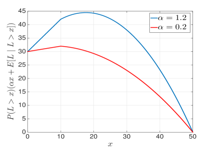
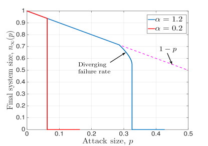
Figure 1: (Color online) We demonstrate the distinction between an abrupt first-order rupture, and a first-order rupture that is preceded by a diverging failure rate. $p_{L}(x)$ is assumed to be of uniform density over the range $[L_{\textrm{min}},L_{\textrm{max}}]=[10,50]$. In both plots, Red curves stand for the case where $\alpha=0.2$, whereas Blue curves represent $\alpha=1.2$. Figure 1 shows ${\mathbb{P}}\left[{L>x}\right]\left(\alpha x+{\mathbb{E}}\left[{L~{}|~{}L>x}\right]\right)$, whereas Figure 1 plots the corresponding variation of $n_{\infty}(p)$ with attack size $p$. We observe that for $\alpha=0.2$ (Red), ${\mathbb{P}}\left[{L>x}\right]\left(\alpha x+{\mathbb{E}}\left[{L~{}|~{}L>x}\right]\right)$ takes its maximum at the point $x=L_{\textrm{min}}=10$. As a result, we see an abrupt first-order transition of $n_{\infty}(p)$ as it suddenly drops to zero at the point $p=p^{\star}=0.0625$, while decaying linearly as $1-p$ up until that point. The case where $\alpha=1.2$ is clearly different as ${\mathbb{P}}\left[{L>x}\right]\left(\alpha x+{\mathbb{E}}\left[{L~{}|~{}L>x}\right]\right)$ is now maximized at $x=17.6>L_{\textrm{min}}$. As expected from our discussion, this ensures that the total failure of the system occurs after a diverging failure rate is observed. This divergence is clearly seen in Figure 1 where the dashed line corresponds to the $1-p$ curve.

III.3 Rupture Condition

We now know how to compute the final system size $n_{\infty}(p)$ for a given attack size $p$. In many cases, we will be interested in the variation of $n_{\infty}(p)$ as a function of $p$. This will help us understand the response of the system to attacks of varying magnitude. Of particular interest will be to derive the critical attack size $p^{\star}$ such that for any attack with size $p>p^{\star}$, the system undergoes a complete breakdown leading to $n_{\infty}(p)=0$.

From (17) and the discussion that follows, we see that the maximum attack size $p^{\star}$ is related to the global maximum of the function ${\mathbb{P}}\left[{L>x}\right]\left(\alpha x+{\mathbb{E}}\left[{L~{}|~{}L>x}\right]\right)$. In fact, it is easy to see that

$$p^{\star}=1-\frac{{\mathbb{E}}\left[{L}\right]}{\max\limits_{x}\{{\mathbb{P}}\left[{L>x}\right]\left(\alpha x+{\mathbb{E}}\left[{L~{}|~{}L>x}\right]\right)\}}.$$ (18)

The critical point $x^{\star}$ that maximizes the function ${\mathbb{P}}\left[{L>x}\right]\left(\alpha x+{\mathbb{E}}\left[{L~{}|~{}L>x}\right]\right)$ can shed light on the type of the transition that the system undergoes as the attack size increases. First of all, the system will always undergo a first-order (i.e., discontinuous) transition at the point $p^{\star}$. This can be seen as follows: We have $n_{\infty}(p^{\star^{+}})=0$ by virtue of the fact that no $x$ will satisfy (17), and cascading failures will continue until the whole system breaks down. On the other hand, $n_{\infty}(p^{\star^{-}})=(1-p){\mathbb{P}}\left[{L>x^{\star}}\right]>0$ where $x^{\star}$ is the point that maximizes ${\mathbb{P}}\left[{L>x}\right]\left(\alpha x+{\mathbb{E}}\left[{L~{}|~{}L>x}\right]\right)$. We can see why it must hold ${\mathbb{P}}\left[{L>x^{\star}}\right]>0$ via contradiction: ${\mathbb{P}}\left[{L>x^{\star}}\right]=0$ implies that the maximum value of ${\mathbb{P}}\left[{L>x}\right]\left(\alpha x+{\mathbb{E}}\left[{L~{}|~{}L>x}\right]\right)$ is zero, which clearly does not hold since at $x=0$ this function equals ${\mathbb{E}}\left[{L}\right]>0$ by non-negativity of $L$.

An interesting question is whether this first order rupture at the point $p^{\star}$ will have any early indicators at smaller attack sizes; e.g., a diverging failure rate leading to a non-linear decrease in $n_{\infty}(p)$. With $L_{\textrm{min}}>0$, we know from (16) that for $p$ sufficiently small, there will be no cascades and $n_{\infty}(p)$ will decrease linearly as $1-p$. This corresponds to the situations where (17) is satisfied at a point $x\leq L_{\textrm{min}}$, i.e., when ${\mathbb{P}}\left[{L>x}\right]\left(\alpha x+{\mathbb{E}}\left[{L~{}|~{}L>x}\right]\right)$ is linearly increasing with $x$. An abrupt first-order transition is said to take place if the linear decay of $n_{\infty}(p)$ is followed by a sudden discontinuous jump to zero at the point $p^{\star}$. Those cases are reminiscent of the real-world phenomena of unexpected large-scale system collapses; i.e., cases where seemingly identical attacks/failures leading to entirely different consequences.

It is easy to see that an abrupt transition occurs if ${\mathbb{P}}\left[{L>x}\right]\left(\alpha x+{\mathbb{E}}\left[{L~{}|~{}L>x}\right]\right)$ takes its maximum at the point $x=L_{\textrm{min}}$; see Figure 1. In that case, (17) either has a solution at some $x\leq L_{\textrm{min}}$ so that $n_{\infty}(p)=1-p$, or has no solution leading to $n_{\infty}(p)=0$. Under the assumptions enforced here, ${\mathbb{P}}\left[{L>x}\right]\left(\alpha x+{\mathbb{E}}\left[{L~{}|~{}L>x}\right]\right)$ is continuous at every $x\geq 0$. Given that this function is linear increasing on the range $0\leq x\leq L_{\textrm{min}}$, a maximum takes place at $x=L_{\textrm{min}}$ if at that point the derivate changes its sign. We have

$$\frac{d}{dx}\left({\mathbb{P}}\left[{L>x}\right]\left(\alpha x+{\mathbb{E}}\left[{L~{}|~{}L>x}\right]\right)\right)$$ (19)

$$=\frac{d}{dx}\left(\alpha x{\mathbb{P}}\left[{L>x}\right]+{\mathbb{E}}\left[{L\cdot{\bf 1}\left[L>x\right]}\right]\right)$$

$$=\alpha{\mathbb{P}}\left[{L>x}\right]+\alpha x(-p_{L}(x))+\frac{d}{dx}\left(\int_{x}^{\infty}tp_{L}(t)dt\right)$$

$$=\alpha{\mathbb{P}}\left[{L>x}\right]+\alpha x(-p_{L}(x))-xp_{L}(x)$$

$$=\alpha{\mathbb{P}}\left[{L>x}\right]-xp_{L}(x)(\alpha+1)$$ (20)

where in the second to last step we used the Leibniz integral rule. As expected, for $x<L_{\textrm{min}}$, we have ${\mathbb{P}}\left[{L>x}\right]=1$ and $p_{L}(x)=0$, so that the derivative is constant at $\alpha$. For an abrupt rupture to take place, the derivative should be negative at the point $x=L_{\textrm{min}}$; i.e., we need

$$\alpha-L_{\textrm{min}}\cdot p_{L}(L_{\textrm{min}})(\alpha+1)<0,$$

or, equivalently

$$\frac{\alpha}{(\alpha+1)L_{\textrm{min}}}<p_{L}(L_{\textrm{min}}).$$ (21)

It is important to note that (21) ensures only the existence of a local maximum of the function ${\mathbb{P}}\left[{L>x}\right]\left(\alpha x+{\mathbb{E}}\left[{L~{}|~{}L>x}\right]\right)$ at the point $x=L_{\textrm{min}}$. This in turn implies that there will be a first order jump in $n_{\infty}(p)$ at the point where ${\mathbb{E}}\left[{L}\right]/(1-p)=\alpha L_{\textrm{min}}+{\mathbb{E}}\left[{L}\right]$; i.e., at the point $p$ that satisfies (16) with equality. However, for this condition to lead to an “abrupt” first-order breakdown, we need $x=L_{\textrm{min}}$ to be the global maximum. This can be checked by finding all $x$ that make the derivate at (20) zero, and then comparing the corresponding maximum points. If $x=L_{\textrm{min}}$ is only a local maximum, then the system will have a sudden drop in size at the corresponding attack size, but will not undergo a complete failure; the complete failure and the drop of $n_{\infty}(p)$ to zero will take place at a larger attack size where, again there will be a first-order transition; e.g., see Figure 2.

We close by giving the general condition for first-order jumps to take place. We need a change of sign of the derivative at (20), leading to

$$\pm\alpha{\mathbb{P}}\left[{L>x}\right]-xp_{L}(x)(\alpha+1)\bigg{|}_{x=x^{\star^{\pm}}}<0.$$

Equivalently, a first-order jump will be seen for every $x^{\star}$ satisfying

$$p_{L}(x^{\star^{-}})<\frac{\alpha{\mathbb{P}}\left[{L>x^{\star}}\right]}{(\alpha+1)x^{\star}}<p_{L}(x^{\star^{+}}).$$ (22)

IV Results with specific distributions

We analyze a few specific distributions in more details. Namely, we will consider Uniform, Pareto, and Weibull distributions.

IV.1 Uniform distribution

Assume that loads $L_{1},\ldots,L_{N}$ are uniformly distributed over $[L_{\textrm{min}},L_{\textrm{max}}]$. In other words, we have

$$p_{L}(x)=\frac{1}{L_{\textrm{max}}-L_{\textrm{min}}}\cdot{\bf 1}\left[L_{\textrm{min}}\leq x\leq L_{\textrm{max}}\right],$$

so that

$${\mathbb{P}}\left[{L>x}\right] =\frac{L_{\textrm{max}}-x}{L_{\textrm{max}}-L_{\textrm{min}}}{\bf 1}\left[L_{\textrm{min}}\leq x\leq L_{\textrm{max}}\right]$$

$$~{}~{}~{}~{}+{\bf 1}\left[x<L_{\textrm{min}}\right].$$ (23)

We see that over the range $x$ in $[0,L_{\textrm{max}})$, the derivative of ${\mathbb{P}}\left[{L>x}\right]\left(\alpha x+{\mathbb{E}}\left[{L~{}|~{}L>x}\right]\right)$ (see (20)) is either never zero or becomes zero only once at

$$x^{\star}=\frac{\alpha}{2\alpha+1}L_{\textrm{max}},$$

For the latter to be possible, we need $\frac{\alpha}{2\alpha+1}L_{\textrm{max}}\geq L_{\textrm{min}}$. If the opposite condition holds, i.e., if $\frac{\alpha}{2\alpha+1}L_{\textrm{max}}<L_{\textrm{min}}$, then ${\mathbb{P}}\left[{L>x}\right]\left(\alpha x+{\mathbb{E}}\left[{L~{}|~{}L>x}\right]\right)$ is maximized at $x=L_{\textrm{min}}$, and an abrupt first order break down will occur (as $p$ increases) without any preceding diverging failure rate. As expected, the condition $\frac{\alpha}{2\alpha+1}L_{\textrm{max}}<L_{\textrm{min}}$ is equivalent to the general rupture condition (21) and can be written most compactly as

$$\alpha<\frac{L_{\textrm{min}}}{\max\left(L_{\textrm{max}}-2L_{\textrm{min}},~{}0\right)}.$$

It follows that if $L_{\textrm{max}}\leq 2L_{\textrm{min}}$, then an abrupt rupture takes place irrespective of the tolerance factor $\alpha$.

IV.2 Pareto distribution

Distribution of many real world variables are shown to exhibit a power-law behavior, with very large variability Faloutsos et al. (1999); Clauset et al. (2009); Newman (2002); Leicht and D’Souza (2009). To consider power systems where the initial loads of the lines can exhibit high variance, we consider the case where $L_{1},\ldots,L_{N}$ are drawn from a Pareto distribution: Namely, with $b,L_{\textrm{min}}>0$, we set

$$p_{L}(x)=L_{\textrm{min}}^{b}bx^{-b-1}{\bf 1}\left[x\geq L_{\textrm{min}}\right].$$

To ensure that ${\mathbb{E}}\left[{L}\right]$ is finite, we also enforce that $b>1$; in that case we have ${\mathbb{E}}\left[{L}\right]=\frac{bL_{\textrm{min}}}{b-1}$. Then, the condition for an abrupt first order rupture (21) gives

$$\frac{\alpha}{(\alpha+1)L_{\textrm{min}}}<L_{\textrm{min}}^{b}bL_{\textrm{min}}^{-b-1},$$

or, equivalently $\frac{\alpha}{\alpha+1}<b$. With $b>1$, this always holds meaning that when the loads are Pareto distributed, there will always be an abrupt first order rupture at the attack size $p^{\star}=1-\frac{{\mathbb{E}}\left[{L}\right]}{{\mathbb{E}}\left[{L}\right]+\alpha L_{\textrm{min}}}=1-\frac{1}{1+\alpha\frac{b-1}{b}}$. In fact, we can see that this attack will lead to a complete breakdown of the system since for $x\geq L_{\textrm{min}}$, we have

$$\frac{d}{dx}\left({\mathbb{P}}\left[{L>x}\right]\left(\alpha x+{\mathbb{E}}\left[{L~{}|~{}L>x}\right]\right)\right)$$ (24)

$$=\alpha{\mathbb{P}}\left[{L>x}\right]-xp_{L}(x)(\alpha+1)$$

$$=\alpha{L_{\textrm{min}}^{b}}{x^{-b}}-(\alpha+1)xL_{\textrm{min}}^{b}bx^{-b-1}$$

$$={L_{\textrm{min}}^{b}}{x^{-b}}\left(\alpha-b(\alpha+1)\right)$$

$$<0$$

for any $\alpha>0$ and $b>1$. Therefore, it is always the case that $\left({\mathbb{P}}\left[{L>x}\right]\left(\alpha x+{\mathbb{E}}\left[{L~{}|~{}L>x}\right]\right)\right)$ has a unique maximum at $x=L_{\textrm{min}}$, and the abrupt first order rupture completely breaks down the system.

These results show that for a given $L_{\textrm{min}}$ and ${\mathbb{E}}\left[{L}\right]$ with ${\mathbb{E}}\left[{L}\right]>L_{\textrm{min}}$, Pareto distribution is the worst possible scenario in terms of the overall robustness of the power system. Put differently, with $L_{\textrm{min}}$ and ${\mathbb{E}}\left[{L}\right]$ fixed, the robustness curve $n_{\infty}(p)$ for the Pareto distribution constitutes a lower bound for that of any other distribution. From a design perspective, we see that changing the tolerance parameter $\alpha$ will not help in mitigating the abruptness of the breakdown of the system in the case of Pareto distributed loads. On the other hand, the point at which the abrupt failure takes place, i.e., the critical attack size $p^{\star}$ can be increased by increasing $\alpha$.

IV.3 Weibull distribution

The last distribution we will consider is Weibull distribution, which has the form

$$p_{L}(x)=\frac{k}{\lambda}\left(\frac{x-L_{\textrm{min}}}{\lambda}\right)^{k-1}e^{-\left(\frac{x-L_{\textrm{min}}}{\lambda}\right)^{k}}{\bf 1}\left[x\geq L_{\textrm{min}}\right],$$

with $\lambda,k>0$. The case $k=1$ corresponds to the exponential distribution, and $k=2$ corresponds to Rayleigh distribution. The mean load is given by ${\mathbb{E}}\left[{L}\right]=L_{\textrm{min}}+\lambda\Gamma(1+1/k)$, where $\Gamma(\cdot)$ is the gamma-function. As usual, we check the derivative of $\left({\mathbb{P}}\left[{L>x}\right]\left(\alpha x+{\mathbb{E}}\left[{L~{}|~{}L>x}\right]\right)\right)$ for $x\geq L_{\textrm{min}}$. On that range, we have ${\mathbb{P}}\left[{L>x}\right]=e^{-\left(\frac{x-L_{\textrm{min}}}{\lambda}\right)^{k}}$ so that

$$\frac{d}{dx}\left({\mathbb{P}}\left[{L>x}\right]\left(\alpha x+{\mathbb{E}}\left[{L~{}|~{}L>x}\right]\right)\right)$$

$$=e^{-\left(\frac{x-L_{\textrm{min}}}{\lambda}\right)^{k}}\left(\alpha-(\alpha+1)x\frac{k}{\lambda}\left(\frac{x-L_{\textrm{min}}}{\lambda}\right)^{k-1}\right)$$ (25)

which becomes zero if

$$x(x-L_{\textrm{min}})^{k-1}=\frac{\alpha\lambda^{k}}{(\alpha+1)k}.$$ (26)

This already prompts us to consider the cases $k<1$ and $k>1$ separately. In fact, with $k>1$, we see that $p_{L}(L_{\textrm{min}})=0$ and (21) does not hold regardless of $\alpha$. In addition, there is one and only one $x>L_{\textrm{min}}$ that can satisfy (26). Consequently, for $k\geq 1$ the system will always undergo a second-order transition with a diverging rate of failure before breaking down completely through a first-order transition.

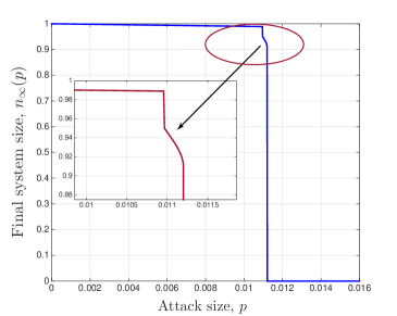
Figure 2: The two stage breakdown of the system is demonstrated, where $L_{1},\ldots,L_{N}$ are drawn from Weibull distribution with $k=0.8$, $\lambda=150$, $L_{\textrm{min}}=10$, $\alpha=0.2$. We plot the relative final size $n_{\infty}(p)$ as a function of the attack size $p$. The Inset zooms in to the region where the system goes through a series of first-order, second-order, and then again a first-order transition.

The case $k<1$ gives an entirely different picture since $p_{L}(L_{\textrm{min}})=\infty$ and (21) always holds regardless of $\alpha$. So, the system will always go through an abrupt first order transition at the attack size $p^{\star}=1-\frac{{\mathbb{E}}\left[{L}\right]}{{\mathbb{E}}\left[{L}\right]+\alpha L_{\textrm{min}}}$. Whether this rupture will entirely breakdown the system depends on the existence of the solutions of (26). It is easy to see that $x(x-L_{\textrm{min}})^{k-1}$ takes its minimum value at $x=L_{\textrm{min}}/k$ and equals to $\frac{L_{\textrm{min}}^{k}}{k}\left(\frac{1-k}{k}\right)^{k-1}$. Thus, if it holds that

$$L_{\textrm{min}}^{k}\left(\frac{1-k}{k}\right)^{k-1}>\frac{\alpha\lambda^{k}}{\alpha+1},$$ (27)

then (26) has no solution and the derivative given at (25) is negative for all $x\geq L_{\textrm{min}}$, meaning that ${\mathbb{P}}\left[{L>x}\right]\left(\alpha x+{\mathbb{E}}\left[{L~{}|~{}L>x}\right]\right)$ is maximized at $x=L_{\textrm{min}}$. Then, the abrupt first order rupture at $p^{\star}=1-\frac{{\mathbb{E}}\left[{L}\right]}{{\mathbb{E}}\left[{L}\right]+\alpha L_{\textrm{min}}}$ will indeed breakdown the system completely. The same conclusion follows if (27) holds with equality by virtue of the fact that (25) is again non-positive for all $x\geq L_{\textrm{min}}$.

On the other hand, if

$$L_{\textrm{min}}^{k}\left(\frac{1-k}{k}\right)^{k-1}<\frac{\alpha\lambda^{k}}{\alpha+1},$$ (28)

then (26) will have two solutions both with $x>L_{\textrm{min}}$. This implies that ${\mathbb{P}}\left[{L>x}\right]\left(\alpha x+{\mathbb{E}}\left[{L~{}|~{}L>x}\right]\right)$ has another maximum at a point $x>L_{\textrm{min}}$. If this maximum is indeed the global maximum (i.e., it is larger than the maximum attained at $x=L_{\textrm{min}}$), then the system will go under two first-order phase transitions before breaking down. First, an abrupt rupture will take place at $p^{\ast}=1-\frac{{\mathbb{E}}\left[{L}\right]}{{\mathbb{E}}\left[{L}\right]+\alpha L_{\textrm{min}}}$. But, this won’t break down the system completely and $n_{\infty}(p^{\ast^{+}})$ will be positive. As $p$ increases further, we will observe a second-order transition with a diverging rate of failure until another first-order rupture breaks down the system completely. We demonstrate this phenomenon in Figure 2, where we set $k=0.8$, $\lambda=150$, $L_{\textrm{min}}=10$, $\alpha=0.2$. We emphasize that this behavior (i.e., occurrence of two first-order transitions) is not immediately warranted under (28). It is also needed that ${\mathbb{P}}\left[{L>x}\right]\left(\alpha x+{\mathbb{E}}\left[{L~{}|~{}L>x}\right]\right)$ has a global maximum at a point $x>L_{\textrm{min}}$.

V Numerical results

We now check the validity of our mean-field analysis for finite number $N$ of power lines via simulations. We will do so with an eye towards comparing the robustness of power systems under different distributions of loads.

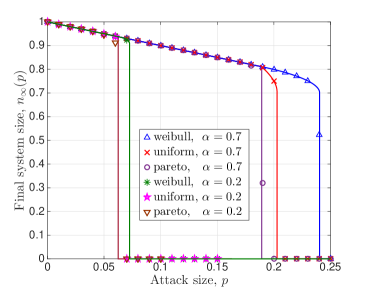
Figure 3: (Color Online). We plot $n_{\infty}(p)$ vs. $p$ under six different cases. Analytical results are represented by lines, whereas empirical results (obtained through averaging over 500 independent runs) are represented by symbols. We set $N=100,000$, $L_{\textrm{min}}=10$, and ${\mathbb{E}}\left[{L}\right]=30$. For the case when $L_{1},\ldots,L_{N}$ follow a Weibull distribution, we take the shape parameter to be $k=2$, leading to a scale parameter $\lambda=22.5676$. We see that numerical results match the analytical results very well.

In the first batch of simulations, we fix the minimum load at $L_{\textrm{min}}=10$ and mean load at ${\mathbb{E}}\left[{L}\right]=30$. These constraints fully determine the load distribution $p_{L}(x)$ in the cases where $p_{L}$ is Uniform (with $L_{\textrm{min}}=10$ and $L_{\textrm{max}}=50$) or Pareto (with $L_{\textrm{min}}=10$ and $b=1.5$). For the case where $p_{L}$ is Weibull, we need to pick $k$ and $\lambda$ such that $\lambda\Gamma(1+1/k)=20$, where $\Gamma(x)=\int_{0}^{\infty}t^{x-1}e^{-t}dt$. We consider $k=2,\lambda=22.5676$ as an example point.

Our simulation set up is as follows. We fix the number of lines $N$, and generate $N$ random variables from the given distribution $p_{L}(x)$ corresponding to loads $L_{1},\ldots,L_{N}$. Then, for a given $p$, we perform an attack on $\lceil pN\rceil$ lines that are selected uniformly at random and assume those lines have failed. Next, using the democratic redistribution of loads, we iteratively fail any line whose load exceeds its capacity (which is set to $(1+\alpha)$ times its initial load). We consider two possible tolerance parameters: i) $\alpha=0.2$ and ii) $\alpha=0.7$. The process stops when the system is stable; i.e., all lines have a load below their capacity. Of course, this steady state can be reached at a point where all lines in the system have failed. We record the corresponding fraction of active lines at the steady state. This process is repeated independently 500 times for each $p$, and the average fraction of active lines at the steady state over 500 independent runs gives the empirical value of $n_{\infty}(p)$. We then compare this with the quantity obtained from our analysis in Section III.

Results are depicted in Figure 3. First of all, we see an almost perfect agreement between our mean-field analysis and numerical results. It is worth noting that the fit between analysis and simulations required particularly large values of $N$ in the case of Pareto distribution. For the other two distributions, even $N=5000$ leads to almost perfect agreement. Focusing on two curves corresponding to uniform distribution, we see from Figure 3 that the tolerance parameter $\alpha$ not only changes the maximum attack size $p^{\star}$ that the system can sustain (in the sense of not breaking down entirely), but it can also affect the type of the phase transition. In particular, with $\alpha=0.2$, an abrupt failure takes place at $p^{\star}=0.0625$, whereas with $\alpha=0.7$ the system goes through a second order transition starting with the attack size $p=0.189$, and then breaks down entirely through a first-order jump at $p^{\star}=0.203$.

As expected from our previous discussion, the distribution that leads to the worst robustness is Pareto among all distributions considered here. However, we see that under certain conditions uniform and Weibull distributions can match the poor robustness characteristics of the Pareto distribution; one example is the case shown in Figure 3 with uniform load distribution and $\alpha=0.2$. Finally, we observe that Weibull distribution can lead to a significantly better robustness than Pareto and Uniform distribution, under the same mean and minimum load.

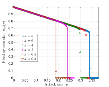
Figure 4: (Color Online). We plot $n_{\infty}(p)$ vs. $p$ when $L_{1},\ldots,L_{N}$ follow a Weibull distribution with $L_{\textrm{min}}=10$, ${\mathbb{E}}\left[{L}\right]=30$. We set $N=100,000$ and $\alpha=0.7$. Analytical results are represented by lines, whereas empirical results (obtained through averaging over 500 independent runs) are represented by symbols. Again, we see that numerical results match the analytical results pretty well.

The last observation worths investigating further. In particular, even when $L_{\textrm{min}}$ and ${\mathbb{E}}\left[{L}\right]$ are fixed, the Weibull distribution has another degree of freedom; i.e., parameters $k$ and $\lambda$ are arbitrary subject to the condition that $\lambda\Gamma(1+1/k)={\mathbb{E}}\left[{L}\right]$. In order to understand the effect of the shape parameter $k$ in the robustness of power systems under Weibull distributed loads, we ran another set of simulations with $N=100,000$, $\alpha=0.7$, $L_{\textrm{min}}=10$, ${\mathbb{E}}\left[{L}\right]=30$, and $\lambda=\frac{20}{\Gamma(1+1/k)}$ for various values of $k$. Results are depicted in Figure 4 where again analytical results are represented by lines and empirical results (obtained through averaging over 500 independent runs) are represented by symbols. We again observe an excellent match between analytical and numerical results. We remark that with the given parameter setting, the cases where $k\leq 1$ all result in the same robustness behavior with an abrupt first-order rupture at $p=0.189$.

More importantly, we see that the robustness of the system improves as the parameter $k$ increases. It is known that as $k$ gets larger the Weibull distribution gets closer and closer to a Dirac delta distribution centered at its mean. In other words, as $k$ goes to infinity the Weibull distribution converges to a degenerate distribution and loads $L_{1},\ldots,L_{N}$ will all be equal to the mean ${\mathbb{E}}\left[{L}\right]$. This naturally prompts us to ask whether a degenerate distribution of loads is the universally optimum strategy among all possible distributions with the same mean ${\mathbb{E}}\left[{L}\right]$, with optimality criterion being the maximization of robustness against random attacks or failures. Here, a natural condition for maximization of robustness would be to maximize the critical attack size $p^{\star}$. We answer this question, in the affirmative, in the next section.

VI Optimal load distribution

To drive the above point further and to better understand the impact of the shape parameter $k$ on the system robustness, we now plot the maximum attack size $p^{\star}$ as a function of $k$ under the same setting; see Figure 5. Namely, we let $L_{1},\ldots,L_{N}$ follow a Weibull distribution with $L_{\textrm{min}}=10$, and $\lambda=20/\Gamma(1+1/k)$ so that ${\mathbb{E}}\left[{L}\right]=30$. We see from Figure 5 that, in all choices of $\alpha$ considered here, the maximum attack size $p^{\star}$ is monotone increasing with $k$; note that $p^{\star}$ is seen to be constant over the range $0<k\leq 1$. It is also evident from Figure 5 that $p^{\star}$ tends to converge to a fixed value as $k\to\infty$. On the other hand, with $k\to\infty$, we know that Weibull distribution converges to a Dirac delta distribution centered at ${\mathbb{E}}\left[{L}\right]$. It is therefore of interest to check whether $p^{\star}$ is always maximized by choosing all loads $L_{1},\ldots,L_{N}$ equally, i.e., by choosing $p_{L}(x)$ to be a degenerate distribution with mean ${\mathbb{E}}\left[{L}\right]$ and zero variance.

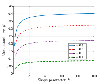
Figure 5: (Color Online). We plot the maximum attack size $p^{\star}$, when $L_{1},\ldots,L_{N}$ follow a Weibull distribution with $L_{\textrm{min}}=10$, ${\mathbb{E}}\left[{L}\right]=30$, as a function of the shape parameter $k$ of the Weibull distribution. We set $N=100,000$ and consider four tolerance parameters $\alpha=0.1,0.3,0.5,0.7$. The curves correspond to analytical results computed directly from (18).

Let $p_{L}(x)$ be an arbitrary distribution with mean ${\mathbb{E}}\left[{L}\right]$, and assume that $p_{L}(x)=0$ for $x\leq 0$; i.e., that $L$ is non-negative. Recall that maximum attack size $p^{\star}$ is given by (18) and observe that

$${\mathbb{P}}\left[{L>x}\right]\left(\alpha x+{\mathbb{E}}\left[{L~{}|~{}L>x}\right]\right)$$

$$=\alpha x{\mathbb{P}}\left[{L>x}\right]+{\mathbb{E}}\left[{L\cdot{\bf 1}\left[L>x\right]}\right]$$

$$\leq\alpha{\mathbb{E}}\left[{L}\right]+{\mathbb{E}}\left[{L\cdot{\bf 1}\left[L>x\right]}\right]$$ (29)

$$\leq(\alpha+1){\mathbb{E}}\left[{L}\right],$$ (30)

for any $x\geq 0$. In (29) we used the Markov Inequality (Papoulis and Pillai, 2002, p. 151), i.e., the fact that ${\mathbb{P}}\left[{L>x}\right]\leq{\mathbb{E}}\left[{L}\right]/x$ for any non-negative random variable $L$ and $x\geq 0$. Reporting (30) into (18), we get

$$p^{\star}\leq 1-\frac{{\mathbb{E}}\left[{L}\right]}{(\alpha+1){\mathbb{E}}\left[{L}\right]}=\frac{\alpha}{\alpha+1}.$$ (31)

This shows that the maximum attack size can never exceed $\frac{\alpha}{\alpha+1}$ under any choice of load distribution. On the other hand, consider the case where $p_{L}(x)=\delta({\mathbb{E}}\left[{L}\right])$ with $\delta(\cdot)$ denoting a Dirac delta function. This implies that $L_{1}=\cdots=L_{N}={\mathbb{E}}\left[{L}\right]$. Let $p^{\star}_{\textrm{dirac}}$ denote the corresponding maximum attack size. With $x={\mathbb{E}}\left[{L}\right]^{-}$, we have ${\mathbb{P}}\left[{L>x}\right]=1$ and ${\mathbb{E}}\left[{L\cdot{\bf 1}\left[L>x\right]}\right]={\mathbb{E}}\left[{L}\right]$. Thus,

$$\lim_{x\uparrow{\mathbb{E}}\left[{L}\right]}\alpha x{\mathbb{P}}\left[{L>x}\right]+{\mathbb{E}}\left[{L\cdot{\bf 1}\left[L>x\right]}\right]=(\alpha+1){\mathbb{E}}\left[{L}\right]$$

so that

$$\max_{x}\{{\mathbb{P}}\left[{L>x}\right]\left(\alpha x+{\mathbb{E}}\left[{L~{}|~{}L>x}\right]\right)\}\geq(\alpha+1){\mathbb{E}}\left[{L}\right].$$

Invoking (18), this leads

$$p^{\star}_{\textrm{dirac}}\geq\frac{\alpha}{\alpha+1}.$$

But, (31) holds for any distribution and hence is also valid for $p^{\star}_{\textrm{dirac}}$. Combining these, we obtain that

$$p^{\star}_{\textrm{dirac}}=\frac{\alpha}{\alpha+1}.$$ (32)

This establishes that a degenerate distribution is indeed optimal for any given mean value of the load, and the achieved maximum attack size is given by $\alpha/(\alpha+1)$. What is even more remarkable is that, this maximum attack size is independent of the mean load ${\mathbb{E}}\left[{L}\right]$.

It is now clear to what point the curves in Figure 5 tend to converge as $k\to\infty$; they can indeed be seen to get closer and closer to the corresponding value of $\alpha/(\alpha+1)$. We close by demonstrating the variation of the final system size as a function of the attack size, in the case where loads follow a Dirac distribution. We easily see that ${\mathbb{P}}\left[{L>x}\right]\left(\alpha x+{\mathbb{E}}\left[{L~{}|~{}L>x}\right]\right)$ increases linearly for $x<{\mathbb{E}}\left[{L}\right]$ and equals to zero for $x\geq{\mathbb{E}}\left[{L}\right]$. Therefore, the breakdown of the system will always be through an abrupt first order rupture.

This is demonstrated in Figure 6, where it is seen once again that numerical results match the analysis perfectly. Comparing these plots with Figures 3 and 4, we see the dramatic impact that the load distribution has on the robustness of a power system. For instance, with $\alpha=0.2$ and mean load fixed at $30$ we see that maximum attack size that the system can sustain is 6.3% for Pareto and Uniform distributions whereas it is 17% when all loads are equal. Similarly, with $\alpha=0.7$ we see that maximum attack size is 18% for Pareto distribution and 19% for Uniform distribution, while for the Dirac delta distribution, it increases to 41%. These findings suggest that under the democratic fiber bundle-like model considered here, power systems with homogenous loads are significantly more robust against random attacks and failures, as compared to systems with heterogeneous load distribution.

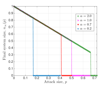
Figure 6: (Color Online). We plot the final system size $n_{\infty}(p)$ as a function of the attack size $p$, when $L_{1}=\cdots=L_{N}={\mathbb{E}}\left[{L}\right]$. For the numerical results, we take $N=100,000$, ${\mathbb{E}}\left[{L}\right]=30$, and consider four tolerance parameters $\alpha=0.2,0.7,1.0,2.0$. Each data point (represented by a symbol) is the result of averaging over 500 independent runs. The lines correspond to analytical results computed directly from (18). We see a perfect agreement between analysis and experiments. In all cases, the system breakdowns abruptly through a first order transition at $p^{\star}=\frac{\alpha}{\alpha+1}.$

VII Conclusion

We studied the robustness of power systems consisting of $N$ lines under a democratic-fiber-bundle like model and against random attacks. We show that the system goes under a total breakdown through a first-order transition as the attack size reaches a critical value. We derive the conditions under which the first-order rupture occurs abruptly without any preceding divergence of the failure rate; those situations correspond to cases where no cascade of failures occurs until a critical attack size is reached, followed by a total breakdown at the critical attack size. Numerical results are presented and confirm the analytical findings. Last but not least, we prove that with mean load fixed, robustness of the power system is maximized when the variation among the line loads is minimized. In other words, a Dirac delta load distribution leads to the optimum robustness.

Our results highlight how different parameters of the load distribution and the power line capacity affect the robustness of the power grid against failures and attacks. To that end, our results can help derive guidelines for the robust design of the power grid. We believe that the results presented here give very interesting insights into the cascade processes in power grids, although through a very simplified model of the grid. The obtained results can be useful in other fields as well, where equal redistribution of flows is a reasonable assumption. Examples include traffic jams, landslides, etc.

There are many open problems one can consider for future work. For instance, the analysis can be extended to the case where the tolerance parameter $\alpha$ is not the same for all lines, but follows a given probability distribution. It would be interesting to see if the robustness is still maximized with a narrow distribution of $\alpha$. It may also be of interest to study robustness against targeted attacks rather than random failures.

References

- Rosas-Casals and Solé (2011) M. Rosas-Casals and R. Solé, International Journal of Electrical Power & Energy Systems 33, 805 (2011).
- Andersson et al. (2005) G. Andersson, P. Donalek, R. Farmer, N. Hatziargyriou, I. Kamwa, P. Kundur, N. Martins, J. Paserba, P. Pourbeik, J. Sanchez-Gasca, et al., Power Systems, IEEE Transactions on 20, 1922 (2005).
- Zhang et al. (2013) G. Zhang, Z. Li, B. Zhang, and W. A. Halang, Physica A: Statistical Mechanics and its Applications 392, 3273 (2013).
- Tang et al. (2012) Y. Tang, G. Bu, and J. Yi, in Zhongguo Dianji Gongcheng Xuebao(Proceedings of the Chinese Society of Electrical Engineering), Vol. 32 (Chinese Society for Electrical Engineering, 2012) pp. 167–174.
- Buldyrev et al. (2010) S. V. Buldyrev, R. Parshani, G. Paul, H. E. Stanley, and S. Havlin, Nature 464, 1025 (2010).
- Watts (2002) D. J. Watts, Proceedings of the National Academy of Sciences 99, 5766 (2002).
- Kinney et al. (2005) R. Kinney, P. Crucitti, R. Albert, and V. Latora, The European Physical Journal B-Condensed Matter and Complex Systems 46, 101 (2005).
- O’Rourke (2007) T. D. O’Rourke, BRIDGE-WASHINGTON-NATIONAL ACADEMY OF ENGINEERING- 37, 22 (2007).
- Dobson et al. (2007) I. Dobson, B. A. Carreras, V. E. Lynch, and D. E. Newman, Chaos: An Interdisciplinary Journal of Nonlinear Science 17, 026103 (2007).
- Yağan et al. (2012) O. Yağan, D. Qian, J. Zhang, and D. Cochran, IEEE Transactions on Parallel and Distributed Systems 23, 1708 (2012), arXiv:1201.2698v2.
- Pahwa et al. (2014) S. Pahwa, C. Scoglio, and A. Scala, Scientific reports 4 (2014).
- Daniels (1945) H. Daniels, Proceedings of the Royal Society of London. Series A. Mathematical and Physical Sciences 183, 405 (1945).
- Andersen et al. (1997) J. V. Andersen, D. Sornette, and K.-t. Leung, Phys. Rev. Lett. 78, 2140 (1997).
- Overbye et al. (2004) T. J. Overbye, X. Cheng, and Y. Sun, in Proceedings, 37th Hawaii International Conference on System Sciences (2004).
- Stott et al. (2009) B. Stott, J. Jardim, and O. Alsac, Power Systems, IEEE Transactions on 24, 1290 (2009).
- Barabási and Albert (1999) A. L. Barabási and L. Albert, Science 286, 509 (1999).
- Curtin (1993) W. Curtin, Journal of the Mechanics and Physics of Solids 41, 217 (1993).
- Kun et al. (2007) F. Kun, M. Costa, R. Costa Filho, J. Andrade Jr, J. Soares, S. Zapperi, and H. Herrmann, Journal of Statistical Mechanics: Theory and Experiment 2007, P02003 (2007).
- Cohen et al. (2009) D. Cohen, P. Lehmann, and D. Or, Water resources research 45 (2009).
- Pradhan and Chakrabarti (2003) S. Pradhan and B. K. Chakrabarti, International Journal of Modern Physics B 17, 5565 (2003).
- Motter and Lai (2002) A. E. Motter and Y.-C. Lai, Phys. Rev. E 66, 065102 (2002).
- Wang and Chen (2008) W.-X. Wang and G. Chen, Phys. Rev. E 77, 026101 (2008).
- Mirzasoleiman et al. (2011) B. Mirzasoleiman, M. Babaei, M. Jalili, and M. Safari, Physical Review E 84, 046114 (2011).
- Crucitti et al. (2004) P. Crucitti, V. Latora, and M. Marchiori, Phys. Rev. E 69, 045104 (2004).
- da Silveira (1998) R. da Silveira, Phys. Rev. Lett. 80, 3157 (1998).
- Sornette et al. (1997) D. Sornette, K.-T. Leung, and J. Andersen, arXiv preprint cond-mat/9712313 (1997).
- Roy et al. (2015) C. Roy, S. Kundu, and S. Manna, Physical Review E 91, 032103 (2015).
- Rosato et al. (2008) V. Rosato, L. Issacharoff, F. Tiriticco, S. Meloni, S. Porcellinis, and R. Setola, International Journal of Critical Infrastructures 4, 63 (2008).
- Note (1) The case of non-uniform initial loads in democratic fiber bundle model is briefly discussed in Pahwa et al. (2014) in the context of power systems, and some numerical results are provided.
- Dobson et al. (2002) I. Dobson, J. Chen, J. Thorp, B. A. Carreras, and D. E. Newman, in System Sciences, 2002. HICSS. Proceedings of the 35th Annual Hawaii International Conference on (IEEE, 2002) pp. 10–pp.
- Note (2) For convenience, we assume that a line also fails when its load equals its capacity.
- Faloutsos et al. (1999) M. Faloutsos, P. Faloutsos, and C. Faloutsos, in ACM SIGCOMM Computer Communication Review, Vol. 29 (ACM, 1999) pp. 251–262.
- Clauset et al. (2009) A. Clauset, C. R. Shalizi, and M. E. J. Newman, SIAM Rev. 51, 661 (2009).
- Newman (2002) M. E. J. Newman, Phys. Rev. E 66 (2002).
- Leicht and D’Souza (2009) E. A. Leicht and R. M. D’Souza, arXiv:0907.0894v1 [cond-mat.dis-nn] (2009), 0907.0894 .
- Papoulis and Pillai (2002) A. Papoulis and S. U. Pillai, Probability, random variables, and stochastic processes, 4th ed. (Tata McGraw-Hill Education, 2002).