Density-matrix based determination of low-energy model Hamiltonians from ab initio wavefunctions

We propose a way of obtaining effective low energy Hubbard-like model Hamiltonians from ab initio quantum Monte Carlo (QMC) calculations for molecular and extended systems. The Hamiltonian parameters are fit to best match the ab initio two-body density matrices and energies of the ground and excited states, and thus we refer to the method as ab initio density matrix based downfolding (AIDMD). For benzene (a finite system), we find good agreement with experimentally available energy gaps without using any experimental inputs. For graphene, a two dimensional solid (extended system) with periodic boundary conditions, we find the effective on-site Hubbard $U^{*}/t$ to be $1.3\pm 0.2$, comparable to a recent estimate based on the constrained random phase approximation. For molecules, such parameterizations enable calculation of excited states that are usually not accessible within ground state approaches. For solids, the effective Hamiltonian enables large-scale calculations using techniques designed for lattice models.

I Introduction

The reliable simulation of systems for which the large-scale physics is not well-approximated by a non-interacting model, is a major challenge in physics, chemistry, and materials science. These systems appear to require a multi-scale approach in which the effective interactions between electrons at a small distance scale are determined, which then leads to a coarse-grained description of emergent correlated physics. This reduction of the Hilbert space is often known as ”downfolding”. In strongly-correlated systems, the correct effective Hamiltonian is strongly dependent on material-specific properties, motivating the need for a generic accurate method to determine it.

One can loosely categorize downfolding techniques into two strategies. The first strategy is based on performing ab initio calculations and then matching them state by state to the effective model. Alternately, some approaches employ a model for the screening of Coulomb interactions, for which the ab initio single particle wavefunctions provide the relevant inputs. For the purposes of this manuscript, the umbrella term we use for these strategies is ”fitting”. Techniques that fall into this class include the constrained density functional theory Pavirini ; Dasgupta , the constrained random phase approximation (cRPA) Aryasetiawan , fitting spin models to energies Valenti_kagome ; Spaldin , and efforts by one of us Wagner_JCP using reduced density matrices of quantum Monte Carlo (QMC) calculations. The second class is based on Löwdin downfolding Freed ; Zhou_Ceperley ; Tenno and canonical transformation theory Glazek_Wilson ; Wegner ; White_CT ; Yanai_CT ; Watson_Chan , which involves a sequence of unitary transformations on the bare Hamiltonian, chosen in a way that minimize the size of the matrix elements connecting the relevant low energy (valence) space to the high energy one.

Downfolding by fitting has the advantage that it is conceptually straightforward to perform, although it demands an a priori parameterization of the effective Hamiltonian. The methods have been applied to complex bulk systems Imada1 ; Imada2 ; Arya1 ; Arya2 ; Scriven ; Wehling_graphene , but it is only recently that their accuracy is being rigorously checked RPA_Troyer . On the other hand, canonical transformations do not need such parameterizations and can discover the relevant terms in an automated way. However, their application to complex materials remains to be carried out and tested.

Here we propose a scheme which aims to capture the ”best of both worlds”. On the one hand, we retain the simplicity of fitting and on the other we use information from accurate many-body wavefunctions to determine which terms are important. The deviations between the ab initio and model properties allows us to assess the quality of the resultant model and to discover relevant physics from the calculation. Simultaneously, the method cannot depend too much on the quality of the ab initio solution because of the inherent limitations of accuracy, especially for very big system sizes.

Once an effective model Hamiltonian in the reduced Hilbert space is obtained, as is depicted in Fig. 1, it can be used to perform a calculation on a larger system using techniques designed for lattice models dmrg_white ; tps_nishino ; Vidal_MERA ; TPS_review ; Changlani_CPS ; Neuscamman_CPS ; mezzacapo ; Marti ; DMET_2012 ; Chen_DMET ; Sandvik_loops ; Blankenbecler ; Alavi_FCIQMC ; SQMC . This multi-step modeling procedure is needed since the ab initio calculations for a given system size are, in general, computationally more expensive than the equivalent lattice calculations. Large sizes are crucial to study finite size effects, and in turn theoretically establish the presence of a phase. In addition, excited states and dynamical correlation functions have traditionally been difficult in ab initio approaches, but have seen progress for lattice model methods dynamical_dmrg ; Daley_tDMRG ; White_tDMRG .

Figure 1: Schematic for downfolding. The full Hamiltonian H is defined in the space of active (partially occupied), core (mostly occupied) and virtual (mostly unoccupied) orbitals. These orbitals have been arranged according to their energy (E) in the figure. The objective is to map the physics of the original system to that of the effective one, defined only in the active space, with Hamiltonian $\tilde{H}$.

In this paper, we demonstrate a downfolding method that uses data from ab initio QMC techniques to derive an effective coarse-grained Hamiltonian. This method, which we call non-eigenstate ab initio density matrix downfolding (N-AIDMD), uses many-body simulations of non-eigenstates to fit an effective low-energy Hamiltonian. We demonstrate that the method can use wavefunctions of medium quality to derive highly accurate effective Hamiltonians. After demonstrating a simple example, we downfold benzene from a 30-electron problem to a 6-electron one and show that the resulting Hamiltonian reproduces the experimental spectrum well. We also show that the method works for extended systems, by applying it to graphene.

II Methods

In the present section we discuss the methods we used to generate our ab initio data. While most of our discussion is specific to QMC, the quantities used can also be calculated in almost any other wavefunction-based quantum chemistry method.

II.1 Variational and Fixed Node Diffusion Quantum Monte Carlo

Ab initio QMC comprises of a suite of methods that efficiently sample the phase space of $N$ electrons each moving in 3-dimensional real space. When the wavefunction as a function of $3N$ coordinates is known, the phase space can be sampled with variational Monte Carlo (VMC) using Metropolis algorithms. For ground state calculations, the Diffusion Monte Carlo (DMC) method, based on imaginary time evolution of the Schroedinger equation, is formally exact but in practice limited by the numerical sign problem. This problem ceases to exist if one knew the exact location of the nodes (zeroes) of the many-body wavefunction. Thus, the optimal strategy for very accurate calculations is to generate a good trial wavefunction, and optimize its parameters to minimize its variational energy. Then, we use this wavefunction to ”fix the nodes” (which may only approximately correspond to the exact nodes) and perform a DMC calculation under this constraint. This last variant is called the fixed-node DMC (FN-DMC) method and is known to be very accurate for a large variety of systems. While some more details are discussed here, we refer the interested reader to Ref. Foulkes_review, for an exhaustive review of concepts and applications. All the ab initio QMC calculations were carried out with the QWalk package QWALK .

A typical QMC calculation was carried out as follows. First, we perform DFT calculations with the B3LYP B3LYP or PBE functionals PBE using GAMESS GAMESS for molecules or CRYSTAL CRYSTAL for solids. The lowest energy DFT orbitals provide the Slater determinant part of the trial wavefunction. For molecules, a multi-determinantal wavefunction is generated by performing a configuration interaction with singles and doubles excitations (CISD) calculation from the reference Slater determinant. Once this is done, a Jastrow factor $\mathcal{J}$ is introduced, resulting in the ansatz for the trial wavefunction $\psi_{T}$,

$$\psi_{T}(r_{1},r_{2},....r_{N})=\mathcal{J}\sum_{i}d_{i}D_{i}$$ (1)

where $(r_{1},r_{2},....r_{N})$ refers to the coordinates of the electrons (the spin indices, being fixed, have been suppressed), $D_{i}$ are determinants and $d_{i}$ their corresponding coefficients. When we desire eigenstates, the parameters in the Jastrow $\mathcal{J}$ and the coefficients $d_{i}$ are optimized to get the best possible variational energy within the ansatz chosen using a technique introduced by Umrigar and coworkers Umrigar_optimization with an efficient algorithm by Clark et al. Clark_multidet .

The variational energy is calculated via Metropolis sampling of $|\psi_{T}|^{2}$,

$$E_{VMC}\equiv\frac{\langle\psi_{T}|H|\psi_{T}\rangle}{\langle\psi_{T}|\psi_{T}\rangle}=\frac{\int|\psi_{T}({\bf{R}})|^{2}\frac{H\psi_{T}({\bf{R}})}{\psi_{T}({\bf{R}})}\;\;\;d{\bf{R}}}{\int|\psi_{T}({\bf{R}})|^{2}d{\bf{R}}}$$ (2)

where $\bf{R}$ is a compact notation for the coordinates of the electrons and $H\psi_{T}({\bf{R}})/\psi_{T}({\bf{R}})$ is the ”local energy”. With this trial wavefunction we perform FN-DMC to calculate the energy using the mixed (or projected) estimator,

$$E_{DMC}\equiv\frac{\langle\psi|H|\psi_{T}\rangle}{\langle\psi|\psi_{T}\rangle}=\frac{\int\psi_{T}({\bf{R}})\psi({\bf{R}})\frac{H\psi_{T}({\bf{R}})}{\psi_{T}({\bf{R}})}d{\bf{R}}}{\int\psi_{T}({\bf{R}})\psi({\bf{R}})d{\bf{R}}}$$ (3)

where $\psi\equiv\exp(-\beta H)\psi_{T}$ is obtained by a stochastic projection of $\psi_{T}$ under the constraint that $\psi$ and $\psi_{T}$ have the same sign everywhere.

We now discuss measurements in the QMC methods. For a generic operator $\hat{O}$, the pure (VMC) and mixed estimators are computed as,

$$\langle\hat{O}\rangle_{VMC}\equiv\frac{\langle\psi_{T}|\hat{O}|\psi_{T}\rangle}{\langle\psi_{T}|\psi_{T}\rangle}\;\;\;\;\langle\hat{O}\rangle_{mix}\equiv\frac{\langle\psi|\hat{O}|\psi_{T}\rangle}{\langle\psi|\psi_{T}\rangle}$$ (4)

The mixed estimator of an operator is equal to the pure estimator in two cases; (1) when $\psi_{T}$ is the exact wavefunction or (2) when the operator $\hat{O}$ commutes with the Hamiltonian. In more general situations, higher accuracy can be obtained with the extrapolated estimatorCeperley_Kalos_Binder for approximate eigenstates,

$$\langle\hat{O}\rangle_{\text{extrap}}=2\langle\hat{O}\rangle_{\text{mix}}-\langle\hat{O}\rangle_{\text{VMC}}$$ (5)

For accurate wavefunctions, all these estimators must approach the same value.

We will construct effective Hamiltonians using the two-body reduced density matrix (2-RDM) elements, given by the estimator (the normalization has been omitted),

$$\rho_{ijkl} \equiv \langle c_{i}^{\dagger}c_{j}^{\dagger}c_{l}c_{k}\rangle=\sum_{a\neq b}\int\phi^{*}_{k}(r^{\prime}_{a})\phi^{*}_{l}(r^{\prime}_{b})\phi_{i}(r_{a})\phi_{j}(r_{b})\Psi^{*}({\bf{R}^{\prime\prime}_{ab}})\leavevmode\nobreak\ \Psi({\bf{R}})dr^{\prime}_{a}dr^{\prime}_{b}d{\bf{R}},$$ (6)

where ${\bf{R}^{\prime\prime}_{ab}}=(r_{1},r_{2},r^{\prime}_{a}...,r^{\prime}_{b},....r_{N})$ refers to the set of electron coordinates obtained by changing the location of two electrons and $\phi_{i}(r)$ are a chosen set of one-particle wavefunctions (orbitals) indexed by label $i(j,k,l)$. The mixed estimator equivalent of Eq. (6) is obtained like that for the energy. More details of this computation have been previously discussed elsewhere by one of us Wagner_JCP . The chosen set of orbitals is often localized on the atoms; this property makes it convenient to derive Hubbard-like models. We explain their construction next.

II.2 Localized orbitals

Localized orbitals often provide an intuitive way of understanding an electronic system in terms of electron hops and on-site or inter-site repulsions. Thus, many works have been devoted to this subject; ranging from the Linearized Muffin-Tin Orbital (LMTO) method Andersen to the maximally localized Wannier function construction Marzari_Wf . Orbital localization has also been widely discussed in the quantum chemistry literature.

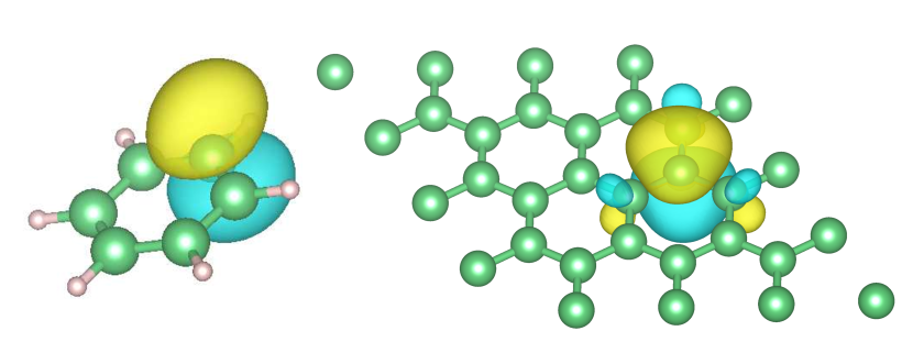
Figure 2: Amplitude isosurface contour for (left) one of the six symmetry equivalent $\pi$ orbitals of the benzene molecule, obtained by localizing three bonding and three anti-bonding orbitals and (right) a representative localized orbital for the $4\times 4$ unit cell of graphene. The colors indicate the sign of the single particle wavefunction.

The idea is to first select a set of orbitals in a certain energy window. For solids these correspond to bands close to the Fermi level, and for molecules these are partially occupied orbitals which constitute the active space. Then, a unitary transformation is performed to optimize a pre-decided metric for localization. In this work, we minimize the spread $S$,

$$S\equiv\sum_{n}\left(\langle\phi_{n}|r^{2}|\phi_{n}\rangle-\langle\phi_{n}|{\bf{r}}|\phi_{n}\rangle^{2}\right)$$ (7)

where $\phi_{n}(r)$ are the desired localized orbitals related to the chosen set of orbitals $\Phi_{i}(r)$ by a unitary transformation, $\phi_{n}(r)=\sum_{i}U_{ni}\Phi_{i}(r)$.

For some systems, as we will see in the case of benzene and graphene, schematically shown in Fig. 2, it is necessary to include unoccupied orbitals to get well-localized orbitals of the right symmetry Hansen . Thus the construction of localized orbitals is not a black-box procedure and may need adaptations based on the specifics of the system.

We note that the optimized parameters of the effective Hamiltonian may, in general, depend on the choice of localized orbitals. However, we have not explored this dependence - our main objective in this paper is to assess the validity of model Hamiltonians with respect to ab initio calculations for a particular choice of single particle basis.

II.3 Lattice model calculations

The lattice model calculations for Hubbard models of benzene and graphene at half-filling were carried out with a combination of our own codes and the freely available QUEST determinantal quantum Monte Carlo package QUEST . For the honeycomb lattice half-filled Hubbard model, the determinantal QMC method is sign problem free and the results are exact up to statistical errors. A time step of $0.1$ was chosen and $\beta$ (the imaginary time) was set to $20$ for every calculation. Measurements were performed for $5000$ sweeps, with an additional $2000$ sweeps being used for equilibration.

III Criteria for a low energy effective Hamiltonian

Our aim is to obtain a low energy effective Hamiltonian defined in the active space of electrons. In this basis, the criteria it must satisfy are:

1. The reduced density matrices (RDM) of the ground and excited states obtained from the ab initio calculation must match with that of the model calculation.

2. The energy spectra of the ab initio and model systems must match in the energy window of interest.

3. The model must be detailed enough to capture the essential physics and yet simple enough to avoid over-parameterization and over-fitting.

The concept of matching RDMs [criterion (a)] has previously appeared in related contexts Acioli ; Zhou_Ceperley ; Changlani_percolation and in work by one of us Wagner_JCP . Most physical properties, such as the charge and spin structure factors, are functions of the 2-RDM. Since it is computationally expensive to calculate high-order RDMs, we use the matching condition only on the 2-RDM, $\rho_{ijkl}\equiv\langle c_{i}^{\dagger}c_{j}^{\dagger}c_{l}c_{k}\rangle$ where $i,j,k,l$ are orbital indices (including space and spin). This criterion automatically ensures that the combined number of electrons occupying the orbitals is equal to those in the model Hamiltonian. If any input state does not have the expected electron number in the active space, it can not be described by the effective Hamiltonian.

The importance of excited state energies used in the fitting [criterion (b)] is highlighted by the fact that the wavefunctions, and their corresponding two-body density matrices, are invariant to many kinds of terms that enter the Hamiltonian. For example, the transformation,

$$H^{\prime}\rightarrow H+\alpha S^{2}+\beta n+\gamma S^{2}n$$ (8)

is, by construction, consistent with all the 2-RDM data for any $\alpha$, $\beta$, $\gamma$ for systems which have definite spin symmetry and particle number. Imposing certain physical constraints on the form of the interactions can reduce the need for this criterion. To give a concrete example, consider wavefunction data generated from the ground state of an unfrustrated Heisenberg spin Hamiltonian on a bipartite lattice  Note1 , $H=J\sum_{\langle i,j\rangle}\bar{S}_{i}\cdot\bar{S_{j}}.$ where $\langle i,j\rangle$ refer to nearest neighbor pairs and $\bar{S}_{i}$ is the spin operator on site $i$. Then adding $\alpha S^{2}$ gives the same reduced density matrices for the ground state, as long as $\alpha$ is small enough to not cause energy crossings i.e. not make an original excited state the new ground state. This additional term has the effect of introducing long-range Heisenberg couplings. Moreover, the effective Hamiltonian is not unique; the Lieb-Mattis model LM $H=S_{A}\cdot S_{B}$ (where $A$($B$) and $S_{A(B)}$ refer to the sublattice and corresponding spin), is also known to reproduce the low-energy limit of the Heisenberg model. Thus, imposing the requirement that the Hamiltonian has the nearest-neighbor form constrains $\alpha$ to zero and picks one particular model. Similar arguments should apply to extended Hubbard models in homogeneous systems where a physical constraint is that the density-density interaction must decrease monotonically with distance between orbitals.

IV Ab Initio Density matrix based Downfolding (AIDMD) procedures

We now discuss two procedures that use density matrices and energies to calculate parameters entering the effective Hamiltonian; both have been schematically depicted in Fig. 3.

IV.1 Eigenstate AIDMD method

In the first method, schematically depicted in Fig. 3(a), eigenstates from an ab initio calculation are used to match density matrices and energies of the corresponding model. The QMC extrapolated estimator is taken to be an accurate representation of the true one. Then the parameters of the model Hamiltonian are obtained by minimizing a cost function that is a linear combination of the energy and density matrix errors,

$$\mathcal{N}\equiv\sum_{s}(E_{s}^{a}-E_{s}^{m})^{2}+f\sum_{s}\sum_{i,j,k,l}(\langle c_{i}^{\dagger}c_{j}^{\dagger}c_{l}c_{k}\rangle^{a}_{s}-\langle c_{i}^{\dagger}c_{j}^{\dagger}c_{l}c_{k}\rangle^{m}_{s})^{2}$$ (9)

where the subscript $s$ is an eigenstate index, $i,j,k,l$ are orbital indices and the superscripts $a$ and $m$ refer to ab initio and model calculations respectively. There is no definite prescription for choosing the weight $f$; a good heuristic is to choose a value that gives roughly the same size of errors for the two terms that enter the cost function. The cost minimization is performed with the Nelder Mead simplex algorithm.

In practice we found that since the number of available eigenstates and the accuracy of true estimators is limited, a second method discussed next is more suited for downfolding.

IV.2 Non-eigenstate AIDMD method

Consider a set of ab initio energy averages $\tilde{E}_{s}$, i.e. expectation values of the Hamiltonian, and corresponding 1- and 2-RDMs $\langle c_{i}^{\dagger}c_{j}\rangle_{s}$, $\langle c_{i}^{\dagger}c_{j}^{\dagger}c_{l}c_{k}\rangle_{s}$ for arbitrary low-energy states characterized by index $s$. Assume a model 2-body Hamiltonian with effective parameters $t_{ij}$ (1-body part) and $V_{i,j,k,l}$ (2-body part) along with a constant term $C$; the total number of parameters being $N_{p}$. Then for each state $s$, we have the equation,

$$\tilde{E}_{s}\equiv\langle H\rangle_{s}=C+\sum_{ij}t_{ij}\langle c_{i}^{\dagger}c_{j}\rangle+\sum_{ijkl}V_{ijkl}\langle c_{i}^{\dagger}c_{j}^{\dagger}c_{l}c_{k}\rangle$$ (10)

where we have made the assumption that the chosen set of operators corresponding to single particle wavefunctions or orbitals, explain all energy differences seen in the ab initio data. The constant $C$ is from energetic contributions of all other orbitals which are not part of the chosen set.

We then perform calculations for $M$ low-energy states which are not necessarily eigenstates. These states are not arbitrary in the sense that they have similar descriptions of the core and virtual spaces. Each state satisfies the criteria (1) its energy average does not lie outside the energy window of interest and (2) the trace of its 1-RDM matches the electron number expected in the effective Hamiltonian.

The objective of choosing a sufficiently big set of states is to explore parts of the low-energy Hilbert space that show variations in the RDM elements. Since the same parameters describe all $M$ states, they must satisfy the linear set of equations,

$$\left(\begin{array}[]{c}\tilde{E}_{1}\\ \tilde{E}_{2}\\ \tilde{E}_{3}\\ ...\\ ...\\ ...\\ ...\\ \tilde{E}_{M}\end{array}\right)=\left(\begin{array}[]{ccccc}1&\langle c_{i}^{\dagger}c_{j}\rangle_{1}&..&\langle c_{i}^{\dagger}c_{j}^{\dagger}c_{l}c_{k}\rangle_{1}&..\\ 1&\langle c_{i}^{\dagger}c_{j}\rangle_{2}&..&\langle c_{i}^{\dagger}c_{j}^{\dagger}c_{l}c_{k}\rangle_{2}&..\\ 1&\langle c_{i}^{\dagger}c_{j}\rangle_{3}&..&\langle c_{i}^{\dagger}c_{j}^{\dagger}c_{l}c_{k}\rangle_{3}&..\\ 1&\langle c_{i}^{\dagger}c_{j}\rangle_{4}&..&\langle c_{i}^{\dagger}c_{j}^{\dagger}c_{l}c_{k}\rangle_{4}&..\\ 1&....&..&..&..\\ 1&....&..&..&..\\ 1&\langle c_{i}^{\dagger}c_{j}\rangle_{M}&..&\langle c_{i}^{\dagger}c_{j}^{\dagger}c_{l}c_{k}\rangle_{M}&..\\ \end{array}\right)\left(\begin{array}[]{c}C\\ t_{ij}\\ ..\\ V_{ijkl}\\ ..\end{array}\right)$$ (31)

which is compactly written as,

$${\bf{E}}=A{\bf{x}}$$ (32)

where ${\bf{E}}\equiv(\tilde{E}_{1},\tilde{E}_{2},...\tilde{E}_{M})^{T}$ is the $M$ dimensional vector of energies, $A$ is the $M\times N_{p}$ matrix composed of density matrix elements and ${\bf{x}}\equiv(C,t_{ij}....V_{ijkl}...)^{T}$ is a $N_{p}$ dimensional vector of parameters. This problem is over-determined for $M>N_{p}$, which is the regime we expect to work in.

Figure 3: Schematic of ab initio density matrix downfolding (AIDMD) methods employed for determining the effective Hamiltonian parameters. (a) In the eigenstate (E)-AIDMD, the reduced density matrices and energies of eigenstates of the model are matched to the ab initio counterparts. (b) The non-eigenstate (N)-AIDMD method uses RDMs and energies of arbitrary low-energy states to construct a matrix of relevant density matrices and performs a least square fit to determine the optimal parameters.

In the case of any imperfection in the model, which is the most common case, the equality will not hold exactly and one must then instead minimize the norm of the error, $\mathcal{N}$:

$$\mathcal{N}\equiv||A\bf{x}-\bf{E}||^{2}$$ (33)

This cost function can be minimized in a single step by using the method of least squares, employing the singular value decomposition of matrix $A$. This matrix also encodes exact (or near-exact) linear dependences. Thus, the quality of the fit is directly judged by assessing (1) the singular values of the $A$ matrix and (2) the value of the cost function itself i.e. the deviations of the input and fitted energies. We will refer to this as the non eigenstate (N)-AIDMD method throughout the rest of the paper. This idea is schematically depicted in Fig. 3(b).

The matrix $A$ gives a very natural basis for understanding renormalization effects. For example, consider a set of wavefunctions that show that the correlator $\langle n_{i}n_{j}\rangle$ does not change significantly. This would lead to the corresponding column of matrix $A$ being identical (up to a scale factor) to the first column of 1’s. Physically, this would correspond to the coupling constant $V_{ijji}$ being irrelevant for the low-energy physics; it can take any value including zero and can be absorbed into the constant shift term. This could also alternatively mean that the input data is correlated and does not provide enough information about $V_{ijji}$, so care must be taken in constructing the set of wavefunctions.

In summary, the N-AIDMD method performs the following operation. The 1- and 2-RDMs and energy expectation values of many non-eigenstate correlated states are calculated. Then, given an effective Hamiltonian parameterization, linear equations (32) are constructed and solved. Standard model fitting principles apply, and we can evaluate the goodness of fit to determine whether a given effective Hamiltonian can sufficiently describe the data.

IV.3 Generating states for AIDMD methods

We now address the central issue of generating states to be used as inputs for the AIDMD methods.

For the E-AIDMD, the near-eigenstates were obtained by performing CISD calculations with multiple roots and optimizing a multi-determinant Jastrow wavefunction with each CISD guess as a starting point. This is known to be approximate, especially for higher excited states. It is the inherent uncertainty about the accuracy of this procedure, along with the fact that only a small number of eigenstates are accessible, that limits the utility of E-AIDMD.

From the point of view of the N-AIDMD method too, automating the construction of the database of wavefunctions may not be completely straightforward and here we offer some heuristics for doing this within QMC methods. We re-emphasize that any state described by the effective Hamiltonian must be one that does not involve large contributions from the core and virtual orbitals i.e. single particle degrees of freedom outside the chosen active space. This check can be imposed at the ab initio level by monitoring the RDMs, for example, the trace of the 1-RDM taken over the active orbitals must equal the number of electrons in the effective Hamiltonian description.

One way to generate new states is to perturb near-eigenstates. For example, after optimizing the multi-determinantal-Jastrow trial wavefunction, we artificially change the determinantal coefficients by small amounts. This procedure changes the nodal surface and gives energies close to, but different from, the optimized ground state. A second source of data is spin excitations of the DFT reference Slater determinant, generated within the space of orbitals that play an important role in the active space; for benzene and graphene these involve the Kohn-Sham orbitals with $\pi$ symmetry. Finally, in the case of extended systems, we chose a linear combination of determinants which, in spite of being not size-extensive, reveal additional properties of the effective Hamiltonian.

IV.4 Quantum Monte Carlo specific adaptation

The formalism introduced above applies to any method that calculates energies and density matrices. In this paper, all the expectation values entering the $A$ matrix are calculated for the chosen low-energy wavefunctions by Monte Carlo sampling.

Once this database of states has been generated, we perform two independent calculations to estimate the parameters, one using variational and the other using mixed estimators. In the latter case, we modify the linear equations (32) by using $E_{s}=\langle{\psi_{T}}^{s}|H|{\psi}^{s}\rangle$ and the projected estimates of the density matrix elements i.e. $\langle{\psi_{T}}^{s}|c_{i}^{\dagger}c_{j}|{\psi}^{s}\rangle$ and $\langle{\psi_{T}}^{s}|c_{i}^{\dagger}c_{j}^{\dagger}c_{l}c_{k}|{\psi}^{s}\rangle$ in the construction of the $A$ matrix. The implicit normalization of these mixed estimates by $\langle{\psi_{T}}^{s}|\psi^{s}\rangle$ is assumed. This projector formulation is also amenable to coupled-cluster calculations which work with projected energies and density matrices.

The bias arising out of fixing the nodes of the projected wavefunction does not affect our formulation. This is because the method regards $\psi\psi_{T}$ as some arbitrary positive sampling function associated with a low energy state, and it is this same distribution that is used for the evaluation of the density matrix elements. Each such distribution provides a linear equation encoding the relationship between the FN-DMC energy and the projected density matrix elements and the unknown parameters. Up to errors from statistical uncertainties and from the assumption of the form of the Hamiltonian, this relationship is exact.

However, the value of the optimal parameters does depend on the choice of method. For example, for the benzene molecule presented in section VI, the VMC and FN-DMC parameter values agree with each other up to $10\%$; the largest discrepancy is due to different constant terms. This discrepancy is expected, because VMC does not provide an accurate description of the core and virtual spaces.

Ideally, only the FN-DMC calculations should be used to estimate the parameters. However, the mixed estimator in FN-DMC is biased because of the inaccuracy of the trial wavefunction. Thus, we propose a better estimator for the parameters,

$$p=2p_{D}-p_{V}$$ (34)

where $p$ is the true parameter, and $p_{D}$ and $p_{V}$ are the corresponding parameters obtained from FN-DMC and VMC calculations. The details of this result are explained in Appendix A.

V Simple application: Hubbard to Heisenberg model

To demonstrate our formalism for a simple example, we consider the two site Hubbard model and fit information from the lowest two states to a Heisenberg model.

We analytically solve for all four eigenstates of the Hamiltonian,

$$H=-t\sum_{ij}c_{i,\sigma}^{\dagger}c_{j,\sigma}+\text{h.c.}+U\sum_{i}n_{i,\uparrow}n_{i,\downarrow}$$ (35)

for two opposite spin electrons on two sites, where $t$ is the hopping, $U$ is the Hubbard on-site interaction. The Hilbert space on a single site (orbital) is spanned by four states $|0\rangle$ (unoccupied), $|\uparrow\rangle$ (single up occupied), $|\downarrow\rangle$ (single down occupied), $|\uparrow\downarrow\rangle$ (doubly occupied). For completeness, we discuss some features of the solution method below.

First notice that the triplet state $|\psi_{t}\rangle\equiv\frac{|\uparrow\;\;\downarrow\rangle-|\downarrow\;\;\uparrow\rangle}{\sqrt{2}}$ with energy $E_{t}=0$ and the state $|\psi_{d}\rangle\equiv\frac{|\uparrow\downarrow\;\;0\rangle-|0\;\;\uparrow\downarrow\rangle}{\sqrt{2}}$ with energy $E_{d}=U$, are exact eigenstates of the problem independent of the values of $t$ and $U$.

To get the other two states, write the Hamiltonian in the basis of $|\psi_{s}\rangle\equiv\frac{1}{\sqrt{2}}\left(|\uparrow\;\;\downarrow\rangle+|\downarrow\;\;\uparrow\rangle\right)$ and $|{\psi_{d}}^{{}^{\prime}}\rangle\equiv\frac{1}{\sqrt{2}}\left(|\uparrow\downarrow 0\rangle+|0\uparrow\downarrow\rangle\right)$,

$$H=\left(\begin{array}[]{cc}0&-2t\\ -2t&U\\ \end{array}\right)$$ (38)

Then diagonalizing it, we get the energies to be,

$$E_{\pm}=\frac{U\pm\sqrt{U^{2}+16t^{2}}}{2}$$ (39)

The lowest energy corresponds to the singlet, $E_{-}$ and the corresponding eigenvector is

$$|\psi_{-}\rangle=\frac{2t}{\sqrt{4t^{2}+{E_{-}}^{2}}}|\psi_{s}\rangle-\frac{E_{-}}{\sqrt{4t^{2}+{E_{-}}^{2}}}|{\psi_{d}}^{{}^{\prime}}\rangle$$ (40)

with the next excited state being the triplet $|\psi_{t}\rangle$.

We choose the Heisenberg form to fit to

$$\tilde{H}=C+JS_{1}\cdot S_{2}$$ (41)

To determine the parameters $C$ and $J$, form the $2\times 2$ $A$ matrix with the lowest two energy states,

$$\left(\begin{array}[]{c}E_{-}\\ E_{t}\\ \end{array}\right)=\left(\begin{array}[]{cc}1&\frac{1}{4+(E_{-}/t)^{2}}\\ 1&-3/4\\ \end{array}\right)\left(\begin{array}[]{c}C\\ J\\ \end{array}\right)$$ (42)

Using derived values of $E_{s}$ and $E_{t}=0$, we get,

$$J=\frac{E_{s}(4+(E_{-}/t)^{2})}{4+\frac{3}{4}(E_{-}/t)^{2}}$$ (43)

which to lowest order in $t/U$ is $J=-4t^{2}/U$.

Observe that the correlator for $\langle S_{i}\cdot S_{j}\rangle$ is not exactly 1/4 but only approximately so. This is expected since the fluctuations from the high-energy states are not exactly zero, if it were, it would be equivalent to exactly block-diagonalizing the Hamiltonian. This exact block diagonalization is not possible in general, unless it is also accompanied with a change in the low energy degrees of freedom entering the model.

If we now rotate the two low energy eigenstates and define the orthogonal linear combinations,

$$|\psi_{1}^{{}^{\prime}}\rangle = p|\psi_{-}\rangle+q|\psi_{t}\rangle$$ (44a)

$$|\psi_{2}^{{}^{\prime}}\rangle = q|\psi_{-}\rangle-p|\psi_{t}\rangle$$ (44b)

and calculate their energies and construct the corresponding $A$ matrix, we get $J$ to be independent of $p$ and $q$. This property is desirable as the method does not hinge on the requirement of eigenstates as inputs.

In terms of canonical transformations (here equivalent to second order perturbation theory), the matrix element of the effective Hamiltonian between the singly occupied states is,

$$\langle\uparrow\downarrow|\tilde{H}|\downarrow\uparrow\rangle = \sum_{n}\frac{\langle\uparrow\downarrow|H|n\rangle\langle n|H|\downarrow\uparrow\rangle}{0-E_{n}}$$ (45)

$$= \frac{-2t^{2}}{U}$$

Since this matrix element must equal $J/2$ in the Heisenberg model we arrive at the same result, namely $J=-4t^{2}/U$ Note2 .

VI Application to a molecule: Benzene

We show the workings of the described AIDMD methods for the benzene molecule. Our choice of system is motivated by its simplicity (one band model and presence of many symmetries) and the availability of experimental energies to compare to.

DFT calculations were first performed in the TZVP basis with Burkatzki-Filippi-Dolg pseudopotentials BFD , using the molecular geometry that corresponds to a B3LYP optimized calculation. These serve as a starting point for the QMC calculations, discussed in the Methods section. In the charge neutral sector, there are a total of 30 electrons (for example, 15 $\uparrow$ and 15 $\downarrow$ for the spin-singlet state) and our objective is to downfold this system to an effective one with 6 electrons (3$\uparrow$, 3 $\downarrow$).

The model Hamiltonian is defined in the space of six $\pi$ orbitals; a representative localized orbital has been shown in Fig. 2. These orbitals were obtained by localizing the highest three occupied and the lowest three unoccupied B3LYP orbitals (from the $S=0$ DFT calculation) with $\pi$ orbital symmetry, a well established procedure in the literature Hansen . The overall phase of these orbitals is adjusted to enable use of parameter symmetries directly when fitting.

Appendix B discusses the QMC data used for fitting and the initial pre-processing to determine the eligibility of states that can be described by a six-$\pi$ orbital Hamiltonian.

VI.1 On-site Hubbard model

We consider the Hubbard model for six orbitals of benzene, given by Eq. (35), where $t$ is used for the nearest-neighbor hopping and $U^{*}$ is the effective on-site Coulomb repulsion. We will discuss multiple ways of using reduced density matrix elements to estimate these parameters.

VI.1.1 Hubbard $U^{*}/t$ from the E-AIDMD method

An estimate of $U^{*}/t$ is obtained by directly matching the half-filled ground state ($S=0$) 2-RDM element corresponding to the ”double occupancy” correlator ($\langle n_{\uparrow}n_{\downarrow}\rangle$) of the ab initio and lattice-model calculations. This element equals $0.25$ for the non interacting case ($U^{*}=0$) and its value reduces for $U^{*}>0$.

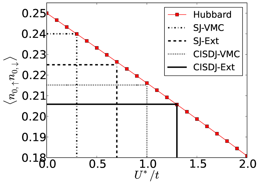
Figure 4: Double occupancy correlator of a single $\pi$ orbital of a six-site ring Hubbard model, as a function of $U^{*}/t$, computed in the half-filled singlet ground state. Comparisons are made with the values from the variational (VMC) and extrapolated (Ext) estimators obtained from ab initio QMC calculations for the benzene molecule with optimized Slater-Jastrow (SJ) and configuration interaction singles doubles-Jastrow (CISDJ) wavefunctions.

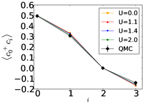
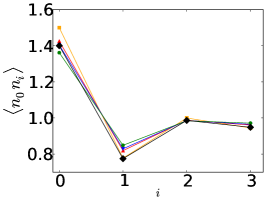
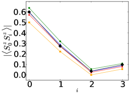
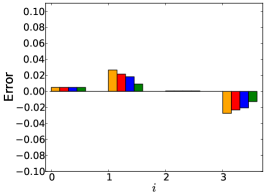
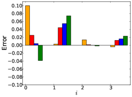
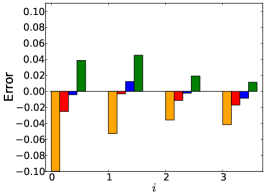
Figure 5: Comparison of correlation functions from ab initio quantum Monte Carlo calculations of the benzene molecule and the six-site Hubbard ring for varying values of $U^{*}/t$. The half-filled ground state has been considered which corresponds to 15 $\uparrow$ and 15 $\downarrow$ electrons in the ab initio calculation and 3 $\uparrow$ and 3 $\downarrow$ electrons in the model calculation. The top panels show the (a) one-body density matrix $\langle c^{\dagger}_{0,\sigma}c_{i,\sigma}\rangle$ (b) density-density correlators $\langle n_{0}n_{i}\rangle$ (c) spin-spin correlators $\langle S_{0}^{z}S_{i}^{z}\rangle$, all as a function of distance ($i$) with respect to a reference site ($0$). Panels (d)-(f) show the same data, but from the point of view of errors of the corresponding model correlation functions with respect to the ab initio data. The one-body density matrix shows relatively small errors for all $U^{*}/t$, but the dependence on $U^{*}/t$ is more pronounced for the density-density and spin-spin correlators. We infer that the value $U^{*}/t\approx 1.4$ reproduces most correlators well, except the nearest-neighbor density-density correlator.

Fig. 4 shows the dependence of $\langle n_{\uparrow}n_{\downarrow}\rangle$, computed in the ground state of the Hubbard model of a six-site ring at half filling, on $U^{*}/t$. The plot also indicates the value of this correlator computed from various wavefunctions and estimators from ab initio QMC calculations of the benzene molecule. The trends are consistent with our expectations; the Slater-Jastrow (SJ) wavefunction at the VMC level underestimates the strength of the effective interactions, which is partly remedied by the extrapolated estimator from FN-DMC. However, the bias (systematic error) is expected to be large because of the considerable difference in the two estimates. This bias is reduced by the multi-determinantal-Jastrow (CISDJ) wavefunction we employed; the difference between the variational and extrapolated estimator is about 5%.

The value of $U^{*}/t$ is found to be extremely sensitive to the precise value of the double occupancy correlator, a change of a few percent (i.e. from $0.24$ to $0.20$) changes our estimate from $\approx 0.3$ to $1.3$ (i.e. a factor of almost $4$). In general, this observation suggests that it is crucial to look at various other elements of the 2-RDM and to look at alternate ways of estimating Hubbard parameters.

In Fig. 5 we compare results of other correlators from extrapolated QMC estimates with those from the on-site Hubbard model on a six site ring for varying values of $U^{*}/t$. We focus on the one-body density matrix $\langle c^{\dagger}_{0,\sigma}c_{i,\sigma}\rangle$ (the values are the same for both spin indices $\sigma$), density-density correlators $\langle n_{0}n_{i}\rangle$ and spin-spin correlators $\langle S_{0}^{z}S_{i}^{z}\rangle$, all as a function of distance ($i$) with respect to a reference site (labelled $0$). The value of $U^{*}/t\approx 1.4$ gives the smallest errors for most observables, except for the nearest-neighbor density-density correlator which favors a value of $U^{*}/t\sim 0$. In the limit that the model is perfect, all estimates must yield the same value; the differences reflect an inadequacy of the on-site Hubbard model in describing all the data. This is evidence for the need for long-range interactions.

VI.1.2 Hubbard $U^{*}/t$ from the N-AIDMD method

As mentioned previously, the idea of matching density matrix elements is useful only for comparing exact eigenstates. However, it is difficult to construct eigenstates with very high accuracy in the ab initio calculations and at times also for the equivalent model for large system sizes. This is why we appeal to the N-AIDMD method, introduced and explained in Sec. IV.2, which is relatively insensitive to the nature of the states input to the method. For charge-neutral benzene, we construct the $A$ matrix by taking various states in a $10$ eV energy window above the ground state using VMC and DMC methods.

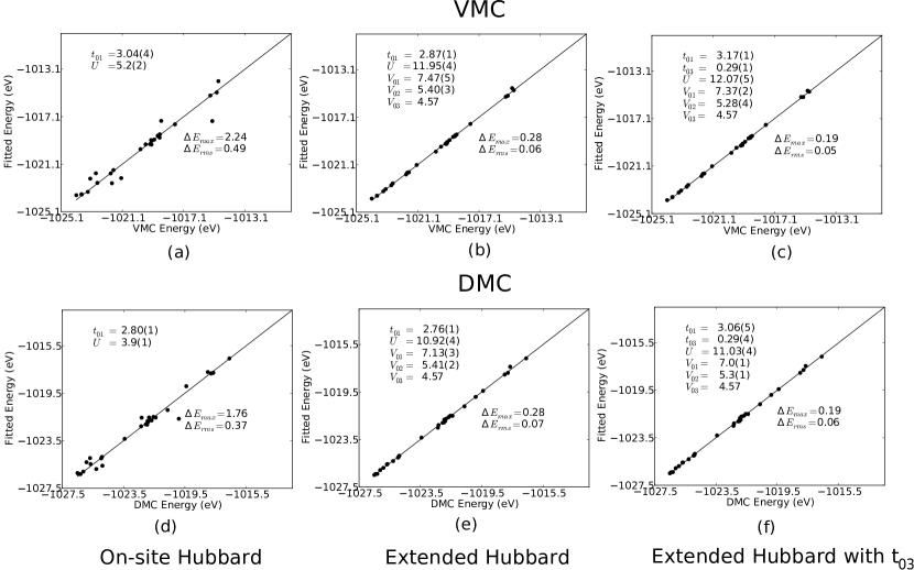
Figure 6: Comparison of ab initio ($x$-axis) and fitted energies ($y$-axis) of the benzene molecule using the N-AIDMD procedure for different model Hamiltonians. The non-eigenstate data is generated by considering various spin excitations and nodal surfaces, all in the same charge sector (30 electrons). The ab initio energy is directly sampled using quantum Monte Carlo methods - for the variational Monte Carlo method (VMC) it corresponds to $\langle\psi_{T}|H|\psi_{T}\rangle/\langle\psi_{T}|\psi_{T}\rangle$ and for the fixed-node diffusion Monte Carlo (DMC) to $\langle\psi_{T}|H|\psi\rangle/\langle\psi_{T}|\psi\rangle$ where $\psi_{T}$ and $\psi$ correspond to trial and projected wavefunctions respectively. The fitted energy is obtained from the optimized parameters by multiplying them by the corresponding ab initio density matrix elements. The top panels (a)-(c) show the VMC results and the bottom ones (d)-(f) show the fixed-node DMC ones. (a) and (d) correspond to the on-site Hubbard model on a six-site ring, (b) and (e) the extended Hubbard model, and (c) and (f) include an additional third-nearest neighbor hopping.

Fig. 6 shows the comparison of the fitted energy and the input VMC or DMC energy. The former is obtained by taking the linear combination of the ab initio VMC or DMC density matrices weighted by the optimized parameters of the effective Hamiltonian. A perfect agreement between the fitted and ab initio input data would correspond to all energies falling exactly on the $y=x$ line. By this measure, the Hubbard model for benzene is reasonable, though not accurate, as is seen in Fig. 6(a) and (d). The presence of significant deviations of the order of $1-2$ eV from the $y=x$ line indicates the need for a more refined model, which we discuss in section VI.2.

The VMC data yields optimal parameters of $t=3.0$ eV and $U^{*}=5.2$ eV ($U^{*}/t=1.7$) and the FN-DMC data gives $t=2.8$ eV and $U^{*}=3.9$ eV ($U^{*}/t=1.4$). The extrapolated estimate of the optimal parameters, $t=2.6$ eV agrees with the value of $t=2.54$ eV reported by Bursill et al. Bursill . The extrapolated value of $U^{*}/t\approx 1.0$ is also broadly consistent with a recently reported estimate Schuler_graphene to within 10-20%.

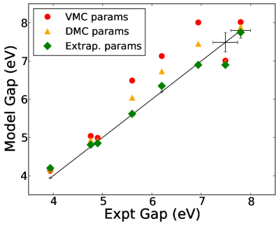
Figure 7: Panel (a) shows the comparison of experimental energy gaps of the benzene molecule and energy gaps of the eigenstates of the extended Hubbard or Parisier-Pople-Parr (PPP) model on a six-site ring using optimized VMC, fixed-node DMC and extrapolated parameters, obtained from the N-AIDMD method. The extrapolated parameters remove, to a large extent, the bias from the other two calculations. All experimental values and associated error-bars are taken from Bursill et al. Ref.[Bursill, ], who used these values to fit to a PPP model with density-density interactions of the Ohno form in Eq. (47). Panel (b) shows the comparison of experimental energy gaps of the benzene molecule and energy gaps of eigenstates for different model Hamiltonians. The on-site Hubbard model and the previous Ohno-parameterized Hamiltonian have at least one significant outlier, which is largely remedied by allowing all $V_{ij}$ and $U$ in the PPP model to be varied.

Parameter	PPP [Ref. Bursill, ]	PPP-VMC	PPP-DMC	PPP-Extrap	$U^{*}$ [Ref. Schuler_graphene, ]	$U^{*}$-VMC	$U^{*}$-DMC
$t$	2.54	$2.87(1)$	$2.76(1)$	2.65(2)	2.54	$3.04(4)$	$2.80(1)$
$U$	10.06	$11.95(4)$	$10.92(4)$	9.89(6)	3.04	$5.2(2)$	$3.9(1)$
$V_{01}$	7.18	$7.47(5)$	$7.13(3)$	6.78(8)	-	-
$V_{02}$	5.11	$5.40(3)$	$5.41(2)$	5.40(4)	-	-
$V_{03}$	4.57	4.57	4.57	4.57	-	-
$U/t$	3.96	4.16(2)	3.96(2)	3.73(3)	1.20	1.7(1)	1.39(5)

Table 1: Model Hamiltonian parameters (in eV) from different downfolding methods, using data from states in the charge neutral sector of benzene. $V_{03}$ sets the constant shift or chemical potential for the interaction terms; its value has been set to match previous semi-empirical fits.

VI.2 Extended Hubbard model

Having established the need for long-range interactions in benzene, we consider the extended-Hubbard or Parisier-Pople-Parr (PPP) model,

$$H=-\sum_{ij}t_{ij}c_{i,\sigma}^{\dagger}c_{j,\sigma}+\text{h.c.}+U\sum_{i}n_{i,\uparrow}n_{i,\downarrow}+\sum_{ij}V_{ij}n_{i}n_{j}$$ (46)

where $U$ is the on-site Hubbard interaction and $t_{ij}$ and $V_{ij}$ are inter-orbital hopping and density-density interactions. We compare our results with Bursill et al Bursill , who considered only a nearest neighbor hopping and took $V_{ij}$ to be of the Ohno form Ohno

$$V_{ij}=\frac{U}{\sqrt{1+(\alpha r_{ij})^{2}}}$$ (47)

where $\alpha$ is a fit parameter and $r_{ij}$ is the spatial separation between nuclei. This parameterization has been widely used in the modelling of various organic polymers. Here do not make any assumptions about the form of the interactions and instead use the N-AIDMD method to determine these parameter values.

We repeat analyses similar to those for the Hubbard model, in addition to carefully looking at the variations in the 1- and 2-RDM matrix elements. This data has been discussed as part of Appendix B and has been shown in Fig. 11. For a parameter to be reliably estimated there should be a large variation in the corresponding density matrix element for different wavefunctions in the low energy space. By this metric, we find that the next nearest neighbor hopping $t_{02}$ is irrelevant in the charge-neutral sector. We thus attempt to fit to a model only with the nearest neighbor $t\equiv t_{01}$ along with $U$, $V_{01}$ and $V_{02}$; $V_{03}$ is not needed as it simply sets the chemical potential.

The inadequacies of the on-site Hubbard model, shown in Figs. 6(a) and (d), are rectified by the extended one, shown in Figs. 6(b) and (e); the maximum energy errors of about $2$ eV are reduced to $\approx 0.3$ eV. The root mean square errors are much smaller as well, reducing from $0.5$ eV to about $0.06$ eV. Adding the next-next nearest neighbor hopping $t_{03}$, shown in Figs. 6(c) and (f), only marginally improves the accuracy of the fit; $t_{03}$ is found to be only about a tenth of the value of $t_{01}$ suggesting that its effects can be largely accounted for by $t_{01}$.

To assess the accuracy of these parameters, we compare the results of the model with experimentally available energies. First, as Fig. 7(a) shows for the extended-Hubbard or PPP model, the extrapolated parameters give an improved agreement with experiment compared to the VMC or FN-DMC parameters. Most energy gaps of this model are in excellent agreement with available experimental energies, the errors are $0.2$ eV or less. The largest outlier at about $7.5$ eV is within $2\sigma$ of the experimental result.

Next, we compare the experimental energies with energy gaps from various model Hamiltonians. While the Hubbard and the Ohno parameterizations reproduce most experimental gaps, especially at low energies, they have at least one significant outlier. These outliers are correctly accounted for by the fitted PPP Hamiltonian, and improved upon by the introduction of $t_{03}$. Owing to the small value of $t_{03}$, more data in the N-AIDMD method may be needed to precisely estimate its value. The extreme sensitivity of the high energy eigenstates to $t_{03}$ may explain the deviation of the model gap from the experimental one at about $7.8$ eV.

We now discuss our parameter values and the errors associated with them; these have been summarized in Table I. While our PPP parameters are generally consistent with the Ohno form, there are some differences of the order of $0.3-0.5$ eV, that improve the quality of the fitted energies. We emphasize that we have not provided any experimental inputs; rather we have used only the QMC data (energies and density matrices) from multiple states to obtain the Hamiltonian parameters.

In order to check the robustness of the fit, we estimated errors in our parameters from a Jackknife analysis. In this scheme half the input states to the N-AIDMD method were randomly discarded and the fit performed with the retained half. Many such randomly generated ensembles of input data were taken and the resultant parameters were averaged over all of these. The difference of the parameters of this reduced data set and those obtained from the full data set provides an estimate of the systematic error, which we report in table I. The other source of error is from statistical noise, which in the present case was found to be much smaller than the systematic error.

VII Application to a solid: Graphene

As an application of the AIDMD methods to solid materials, we consider graphene, a 2D solid of carbon atoms arranged on a honeycomb lattice. Graphene has great potential technological applications, which has spurred much work devoted to understanding it thoroughly graphene_review . In addition, there have been several proposals for engineering exotic phases in graphene Herbut ; Duric ; Ghaemi . That said, it is only recently that systematic studies to estimate the role of electron-electron interactions Wehling_graphene ; Schuler_graphene ; Abbamonte have been carried out. While some of its long-distance properties appear to be adequately described by a tight-binding model, the short range features, crucial for phenomena such as magnetism, require more refined modeling.

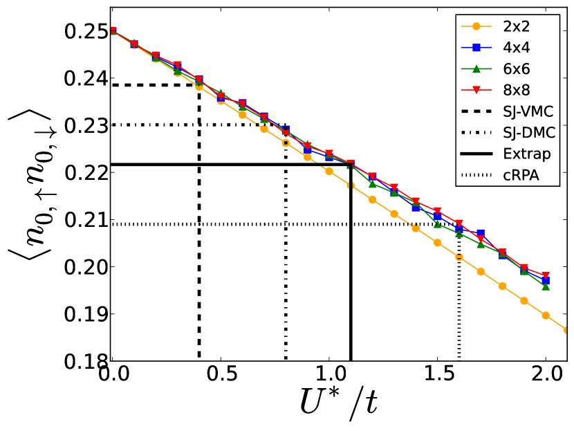
Figure 8: Double occupancy correlator of a single $\pi$ orbital of the $L\times L$ ($L=2,4,6,8$) honeycomb lattice Hubbard model with periodic boundary conditions, as a function of $U^{*}/t$, computed in the half-filled singlet ground state. Comparisons are made with the values from variational (VMC), mixed (DMC) and extrapolated (Ext) estimators obtained from ab initio QMC calculations on $4\times 4$ graphene using an optimized Slater-Jastrow (SJ) trial wavefunction. The cRPA estimate from Ref.[Schuler_graphene, ] is also shown.

Figure 9: Comparison of ab initio ($x$-axis) and fitted energies ($y$-axis) of the $3\times 3$ periodic unit cell of graphene, using the N-AIDMD procedure. The non-eigenstate data is generated by considering various spin excitations and nodal surfaces, all in the same charge sector (72 electrons). The ab initio energy is directly sampled using quantum Monte Carlo methods - for the variational Monte Carlo method (VMC) it corresponds to $\langle\psi_{T}|H|\psi_{T}\rangle/\langle\psi_{T}|\psi_{T}\rangle$ and for the fixed-node diffusion Monte Carlo (DMC) to $\langle\psi_{T}|H|\psi\rangle/\langle\psi_{T}|\psi\rangle$ where $\psi_{T}$ and $\psi$ correspond to trial and projected wavefunctions respectively. The fitted energy is obtained from the optimized parameters by multiplying them by the corresponding ab initio density matrix elements. The top panels (a),(b) show the VMC results and the bottom ones (c),(d) show the fixed-node DMC ones. (a) and (c) correspond to the tight binding model on a honeycomb lattice, and (b) and (d) correspond to the on-site Hubbard model.

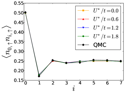
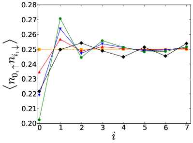
Figure 10: Comparison of correlation functions of the half-filled, unpolarized ground state of $4\times 4$ periodic cell of graphene from ab initio quantum Monte Carlo with those from determinantal quantum Monte Carlo calculations of the honeycomb lattice on-site Hubbard model for various values of $U^{*}/t$. Panel (a) shows the up density - up density correlator $\langle n_{0,\uparrow}n_{i,\uparrow}\rangle\rangle$ and (b) shows the up density - down density correlator $\langle n_{0,\uparrow}n_{i,\downarrow}\rangle$ for the $i^{th}$ neighbor of a reference site (labelled $0$). The like-density correlators depend weakly on $U^{*}/t$ on the scale shown for all $i$. The correlator $\langle n_{0,\uparrow}n_{0,\downarrow}\rangle$ suggests $U^{*}/t\approx 1.2$, but the deviation for $\langle n_{0,\uparrow}n_{1,\downarrow}\rangle$ indicates that the Hubbard model overestimates the nearest-neighbor attraction between electrons of opposite spins.

Early studies modelled graphene as a honeycomb lattice Hubbard model with a $U/t$ estimated to be $\approx 3.8$. This would put graphene on the verge of a metal-insulator transition Sorella_Tosatti ; Sorella_Nature . However, recent results by Wehling et al. realized the importance of long range interactions Wehling_graphene , which renormalize the on-site interaction to an effectively lower value. Schuler et al. Schuler_graphene report the effective $U^{*}/t$ to be $1.6\pm 0.2$, which means graphene lies well in the semimetal phase of the honeycomb lattice Hubbard model.

Setting aside the question of determining all the long range interactions in graphene, we ask what $U^{*}/t$ best describes our ground state QMC data. To do so, we first generated the $\pi$-like Wannier functions within QWalk QWALK , a representative of which has been shown in Fig. 2.

Just as in the case of benzene, we used the fact that the effective strength of the Coulomb interaction $U^{*}/t$ is most sensitive to the 2-RDM element $\langle n_{i,\uparrow}n_{i,\downarrow}\rangle$. For the $4\times 4$ unit cell with periodic boundary conditions, and using optimized Slater Jastrow wavefunctions, the extrapolated value is found to be $0.221(5)$ corresponding to a $U^{*}/t\approx 1.1(1)$. This estimate of $U^{*}/t$ is obtained from comparisons to lattice determinantal QMC calculations, which were carried out for sizes ranging from $2\times 2$ to $8\times 8$ to check for finite-size effects. As Fig. 8 shows, the $2\times 2$ unit cell is distinctly different from the larger unit cells and the finite-size errors in the double occupation correlator are negligible beyond sizes $L\geq 4$. The finite size effects for other short range correlation functions (not shown) are also negligible beyond $L\geq 4$.

We also calculated many non-eigenstates for $3\times 3$ graphene in an energy window $3$ eV above the ground state. Fig. 9 shows the VMC and FN-DMC energy fits to tight-binding and Hubbard models. The hopping $t$ for the tight-binding model is found to be in the range of $2.2$ to $2.8$ eV, as is indicated in Figs. 9(a) and (c). However, a precise estimate of this parameter is not particularly meaningful because the model is inadequate at capturing many states, particularly spinful excitations, in this energy window. We note that a value of $t=2.80$ eV Schuler_graphene has been previously calculated with DFT methods.

Figs. 9(b) and (d) show that the Hubbard model reduces the errors of the tight-binding model, and the value of $U^{*}/t$ is found to be in the range of $1.9$ (VMC) to $1.3$ (FN-DMC). The latter estimate is expected to be more accurate and hence closer to the true value of $U^{*}/t$ in a small energy window associated with the ground state. We also note that this value is within $2\sigma$ of the value derived from the constrained RPA parameters Schuler_graphene . However the Hubbard model too has outliers of about $0.4$ eV, which are large for an accurate model of a solid material.

This inadequacy is confirmed by assessing various correlators in the half filled ground state. Fig. 10 shows the up density-up density and up density- down density correlators as a function of distance between carbon atoms. On the scale of Fig. 10(a) (and well within the accuracy of our calculations) the like spin correlations were captured well for all values of $U^{*}/t$ in the range from $0$ to $2$. However, as Fig. 10(b) shows, the Hubbard model for large $U^{*}/t$ tends to exaggerate the the effective interaction between the two electron spin flavors at small separations. In particular, the nearest neighbor unlike spin density-density correlator is found to be in better agreement with $U^{*}/t\sim 0$ than any finite value. This, just like the case of benzene, suggests the need for longer range interactions in the model. There are also small deviations between the ab initio QMC and the Hubbard model results at longer distances. These correlations do not depend significantly on $U^{*}/t$ and these data in isolation do not rule out any model.

VIII Conclusion

We have demonstrated ab initio density matrix downfolding (AIDMD) methods where ab initio quantum Monte Carlo (QMC) data is used to fit simple effective Hamiltonians. We have elaborated on the fitting procedures and the intricacies of the QMC method needed to perform calculations. The limitations of the model were judged by assessing the quality of the fitted energies and 2-body density matrices. This feature is useful for constructing refined models needed for the accurate simulation of real materials.

For the benzene molecule, while the on-site Hubbard model with $U^{*}/t\approx 1.2\pm 0.2$ was able to capture most features of the QMC ground state data, the deviations of the density matrices revealed the need for longer range interactions. Including these interactions improved the agreement of the model with both the QMC results and the experimental data. This effective Hamiltonian parameterization could be used to calculate low-frequency response functions and to check semi-empirical methods.

Since QMC calculations use size-consistent wavefunctions for extended systems and scale favorably, we believe the type of calculations presented here will be a promising alternative to DFT-based downfolding approaches for solid materials. Our demonstration for the single band model of graphene yielded an effective $U^{*}/t=1.3\pm 0.2$, in the same range as a recently reported estimate based on the constrained-RPA method Schuler_graphene . We leave a more detailed characterization of interactions in graphene to future work.

In more complicated materials, where the form of the Hamiltonian is unclear, we suggest that the dominant terms can be obtained from canonical transformation theory followed with an accurate fit to the QMC data. In this spirit, it will also be useful to compare the predictions of the proposed AIDMD schemes with other complementary proposals for downfolding Zhang ; Zgid ; Watson_Chan .

Finally, we remark that previously unsolved model Hamiltonians are now being accurately treated with tensor network methods Stoudenmire_White_2D_DMRG ; Corboz_Rice_Troyer . With parallel advances in the ab initio QMC simulation of high-temperature superconductors Wagner_cuprates ; Krogel_cuprates , a clear future direction is to deduce more refined models for these compounds, using the ideas discussed in the paper.

IX Acknowledgement

We thank David Ceperley, Cyrus Umrigar, Garnet Chan, Shiwei Zhang, Steven White, Gabriel Kotliar, Bryan Clark, Norman Tubman, Victor Chua and Miles Stoudenmire for discussions. We would also like to thank Cyrus Umrigar for running very useful checks against his quantum Monte Carlo code (CHAMP) in the early stages of this work. We acknowledge support from SciDAC grant DE-FG02-12ER46875. Computational resources were provided by the DOE INCITE SuperMatSim program and the Taub campus cluster at the University of Illinois at Urbana-Champaign.

X Appendix A: Estimation of true effective Hamiltonian parameters from VMC and FN-DMC calculations

In section IV.4, we discussed the discrepancy between parameters obtained from VMC and FN-DMC. This is attributed to the inability of the trial wavefunctions used in VMC to provide an accurate description of the core and virtual spaces.

As mentioned in the text, ideally, only the FN-DMC calculations should be used to estimate the parameters. However, the mixed estimator in FN-DMC is biased because of the inaccuracy of the trial wavefunction. To minimize this bias, we propose estimators which combine FN-DMC and VMC parameters.

Consider a trial VMC wavefunction $\psi_{T}$ which deviates from the DMC wavefunction $\psi$ by a small amount $\delta\psi_{h}$ orthogonal to $\psi_{T}$ i.e.,

$$|\psi\rangle=|\psi_{T}\rangle+\delta|\psi_{h}\rangle$$ (48)

To obtain the parameter $p$ coupled to an operator $\rho_{p}$ in the effective Hamiltonian i.e.

$$H=\sum_{p}p\;\;\rho_{p}$$ (49)

we take partial derivatives with respect to the change of a density matrix element i.e.

$$p=\frac{\partial\langle\psi|H|\psi\rangle}{\partial\langle\psi|\rho_{p}|\psi\rangle}$$ (50)

Since the pure estimators for projected (DMC) wavefunctions are not easily evaluated in QMC, we use other estimators using which we indirectly obtain $p$.

The parameter obtained from the mixed estimators within FN-DMC, is formally defined as,

$$p_{D}=\frac{\partial\langle\psi|H|\psi_{T}\rangle}{\partial\langle\psi|\rho_{p}|\psi_{T}\rangle}$$ (51)

On substituting the relation between $\psi$ and $\psi_{T}$ wavefunctions, we get,

$$p_{D}=\left(\frac{\partial\langle\psi|H|\psi\rangle}{\partial\langle\psi|\rho_{p}|\psi\rangle}\right)\left(1-\delta\frac{\partial\langle\psi|H|\psi_{h}\rangle}{\partial\langle\psi|H|\psi\rangle}\right)\left(1-\delta\frac{\partial\langle\psi|\rho_{p}|\psi_{h}\rangle}{\partial\langle\psi|\rho_{p}|\psi\rangle}\right)^{-1}$$ (52)

which to linear order in $\delta$ is,

$$p_{D}\approx p\left(1+\delta\left(\frac{\partial\langle\psi|\rho_{p}|\psi_{h}\rangle}{\partial\langle\psi|\rho_{p}|\psi\rangle}-\frac{\partial\langle\psi|H|\psi_{h}\rangle}{\partial\langle\psi|H|\psi\rangle}\right)\right)$$ (53)

A similar expression for parameters obtained from VMC calculations,

$$p_{V}=\frac{\partial\langle\psi_{T}|H|\psi_{T}\rangle}{\partial\langle\psi_{T}|\rho_{p}|\psi_{T}\rangle}$$ (54)

is derived and leads to the result,

$$p_{V}\approx p\left(1+2\delta\left(\frac{\partial\langle\psi|\rho_{p}|\psi_{h}\rangle}{\partial\langle\psi|\rho_{p}|\psi\rangle}-\frac{\partial\langle\psi|H|\psi_{h}\rangle}{\partial\langle\psi|H|\psi\rangle}\right)\right)$$ (55)

where we have used the hermiticity of the Hamiltonian $H$ and the operator $\rho_{p}$.

On combining equations (53) and (55), to leading order in $\delta$ we get,

$$p=2p_{D}-p_{V}+O({\delta}^{2})$$ (56)

As expected, all estimates are consistent with each other in the limit of exact wavefunctions.

XI Appendix B: QMC data for the benzene molecule

Table II shows the QMC data for several eigenstates of benzene. Most of these states along with many other non-eigenstates constitute our data set for fitting a model.

Spin	DFT	SJ-VMC	SJ-DMC	CISDJ-VMC	CISDJ-DMC	$N_{\uparrow},N_{\downarrow}$	Used in Fit?
0	-37.6303	-37.6229(6)	-37.7213(9)	-37.6352(6)	-37.7259(9)	2.96,2.96	Yes
1	-37.4634	-37.4546(6)	-37.5555(7)	-37.4814(6)	-37.5707(7)	3.94,1.98	Yes
				-37.4561(6)	-37.5479(6)	3.94,1.98	Yes
				-37.4531(6)	-37.5470(6)	3.94,1.98	Yes
2	-37.3203	-37.2987(6)	-37.3974(7)	-37.3141(6)	-37.4020(7)	4.92,1.00	Yes
3	-37.0378	-37.0116(4)	-37.1074(7)	-37.0118(4)	-37.1083(7)	4.88,0.02	No

Table 2: Energy of different spin eigenstates in the charge-neutral sector of benzene from DFT and QMC methods. SJ refers to the Slater Jastrow wavefunctions. CISDJ refers to multi-determinantal Jastrow wavefunctions where the determinants are obtained from a CI-singles doubles calculations and their weights optimized within VMC. All DMC calculations used a time step of 0.01 Ha^-1. The states that had significantly different occupations from the expected values were not used in the fitting as they can not be described by an effective Hamiltonian involving only six $\pi$ orbitals.

The calculations confirm the general expectation that significant energy gains are obtained by improving wavefunctions going from the single-Slater-Jastrow form to the multi-determinantal-Jastrow form (the determinants being selected from a CISD calculation). Moreover, the DMC calculations improve total energies significantly; typically, the DMC values are $2-3$ eV lower than the corresponding VMC value.

The total electron count from the one-body density matrix is assessed to verify the validity of fitting to a six-$\pi$ orbital Hamiltonian. Table II shows that for charge-neutral benzene, the singlet state ($S=0$) has up and down electron counts of 2.96 each, which are close to the expected values of 3,3. For the $S=2$ state, roughly $9$ eV above the ground state, the deviations were slightly larger; the summed occupation numbers were 4.92 and 1.0 in comparison to the expected values of 5 and 1. Since there is a slight deviation of these numbers from integers, we rescale the one and two body density matrices by factors (all slightly greater than 1) that correctly accounts for sum rules for each individual state used in the AIDMD methods.

However, for the $S=3$ state, the electron occupation numbers deviate significantly from the corresponding value in the model; almost by one integer. This indicates that the $S=3$ state is inadequately described by the proposed Hamiltonian and hence can not be used in the fitting procedure. This deviation is not completely unexpected since this state is $\sim 17$ eV above the ground state and a potential high-energy state. Said differently, the active space at this energy scale is considerably different from that assumed for the ground state and its low-energy excitations. Thus, this QMC data suggests that it is only reasonable for the effective Hamiltonian concept to hold only in an energy window of the order of $10$ eV above the ground state.

We now assess some aspects of our non-eigenstate data. As mentioned in the main text, heuristics were used to construct these states. For example, for every near-eigenstate in a symmetry sector that was represented by multi-determinantal Jastrow form, we changed the determinantal coefficients to generate new wavefunctions. We checked the 1-RDM to make sure that it had the correct total electron number (6 electrons) on the localized orbitals that constitute our active space. Moreover, if the change in determinantal coefficients led to an energy-average outside our pre-decided energy window, the new state was discarded from the N-AIDMD procedure.

For the N-AIDMD method, we desire large variations in the density matrix elements for different wavefunctions in the low-energy space, in order to accurately estimate the Hamiltonian parameters. Fig. 11 shows these variations for all relevant density-matrix elements (within FN-DMC) that were needed for estimating the parameters of the extended Hubbard model. $t_{02}$ was found to be irrelevant, as the summed density matrix elements coupling to it were found to not vary significantly (not shown in the plot).

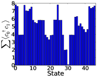
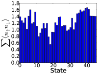
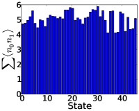
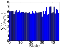
Figure 11: Variation of density matrix elements for various states of the benzene molecule used in the N-AIDMD method. The summation sign $\sum$ indicates a sum over all RDM elements that couple to the same parameter in the lattice model. The panels show (a) the sum over all the nearest neighbor one body density matrix elements summed over both spin types and (b) the sum over on-site double occupancies. (c) and (d) show sums over nearest and next-nearest neighbor density-density correlators respectively. As is discussed in the text, variations in the density matrix elements are needed for the corresponding parameters to be estimated, else they can be taken to be effectively zero.

References

- (1) E. Pavarini et al., Phys. Rev. Lett. 87, 047003 (2001).
- (2) O. K. Andersen and T. Saha-Dasgupta, Phys. Rev. B 62, R16219 (2000).
- (3) F. Aryasetiawan et al., Phys. Rev. B 70, 195104 (2004).
- (4) H. O. Jeschke, F. Salvat-Pujol, and R. Valentí, Phys. Rev. B 88, 075106 (2013).
- (5) N. S. Fedorova, C. Ederer, N. A. Spaldin, A. Scaramucci, arXiv:1412.3702.
- (6) L. K. Wagner, The Journal of Chemical Physics 138, 094106 (2013).
- (7) K. F. Freed, Accounts of Chemical Research 16, 137 (1983).
- (8) S. Q. Zhou and D. M. Ceperley, Phys. Rev. A 81, 013402 (2010).
- (9) S. Ten-no, The Journal of Chemical Physics 138, (2013).
- (10) S. D. Głazek and K. G. Wilson, Phys. Rev. D 48, 5863 (1993).
- (11) F. Wegner, Annalen der Physik 506, 77 (1994).
- (12) S. R. White, The Journal of Chemical Physics 117, (2002).
- (13) T. Yanai and G. K.-L. Chan, The Journal of Chemical Physics 124, (2006).
- (14) T. J. Watson Jr., G. K-L Chan, arXiv:1502.04698.
- (15) M. Hirayama, T. Miyake, and M. Imada, Phys. Rev. B 87, 195144 (2013).
- (16) K. Nakamura, Y. Yoshimoto, Y. Nohara, and M. Imada, Journal of the Physical Society of Japan 79, 123708 (2010).
- (17) F. Nilsson, R. Sakuma, and F. Aryasetiawan, Phys. Rev. B 88, 125123 (2013).
- (18) F. Aryasetiawan, K. Karlsson, O. Jepsen, and U. Schönberger, Phys. Rev. B 74, 125106 (2006).
- (19) E. P. Scriven and B. J. Powell, Phys. Rev. Lett. 109, 097206 (2012).
- (20) T. O. Wehling et al., Phys. Rev. Lett. 106, 236805 (2011).
- (21) Hiroshi Shinaoka, Rei Sakuma, Philipp Werner, Matthias Troyer, arXiv:1410.1276.
- (22) S. R. White, Phys. Rev. Lett. 69, 2863 (1992).
- (23) A. Gendiar, N. Maeshima, and T. Nishino, Prog. Theor. Phys. 110, 691 (2003).
- (24) G. Vidal, Phys. Rev. Lett. 101, 110501 (2008).
- (25) F. Verstraete, V. Murg, and J. Cirac, Advances in Physics 57, 143 (2008).
- (26) H. J. Changlani, J. M. Kinder, C. J. Umrigar, and G. K.-L. Chan, Phys. Rev. B 80, 245116 (2009).
- (27) E. Neuscamman, H. Changlani, J. Kinder, and G. K.-L. Chan, Phys. Rev. B 84, 205132 (2011).
- (28) F. Mezzacapo, N. Schuch, M. Boninsegni, and J. I. Cirac, New J. Phys. 11, 083026 (2009).
- (29) K. H. Marti et al., New Journal of Physics 12, 103008 (2010).
- (30) G. Knizia and G. K.-L. Chan, Phys. Rev. Lett. 109, 186404 (2012).
- (31) Q. Chen et al., Phys. Rev. B 89, 165134 (2014).
- (32) O. F. Syljuåsen and A. W. Sandvik, Phys. Rev. E 66, 046701 (2002).
- (33) R. Blankenbecler, D. J. Scalapino, and R. L. Sugar, Phys. Rev. D 24, 2278 (1981).
- (34) G. H. Booth, A. J. W. Thom, and A. Alavi, J. Chem. Phys. 131, 054106 (2009).
- (35) F. R. Petruzielo et al., Phys. Rev. Lett. 109, 230201 (2012).
- (36) E. Jeckelmann, Phys. Rev. B 66, 045114 (2002).
- (37) A. J. Daley, C. Kollath, U. Schollwöck, and G. Vidal, Journal of Statistical Mechanics: Theory and Experiment 2004, P04005 (2004).
- (38) S. R. White and A. E. Feiguin, Phys. Rev. Lett. 93, 076401 (2004).
- (39) W. M. C. Foulkes, L. Mitas, R. J. Needs, and G. Rajagopal, Rev. Mod. Phys. 73, 33 (2001).
- (40) L. K. Wagner, M. Bajdich, and L. Mitas, Journal of Computational Physics 228, 3390 (2009).
- (41) A.D. Becke, J.Chem.Phys. 98 (1993) 5648-5652; C. Lee, W. Yang, R.G. Parr, Phys. Rev. B 37 (1988) 785-789; S.H. Vosko, L. Wilk, M. Nusair, Can. J. Phys. 58 (1980) 1200-1211; P.J. Stephens, F.J. Devlin, C.F. Chabalowski, M.J. Frisch, J.Phys.Chem. 98 (1994) 11623-11627.
- (42) J. P. Perdew, K. Burke, and M. Ernzerhof, Phys. Rev. Lett. 77, 3865 (1996).
- (43) M.W.Schmidt, K.K.Baldridge, J.A.Boatz, S.T.Elbert, M.S.Gordon, J.H.Jensen, S.Koseki, N.Matsunaga, K.A.Nguyen, S.Su, T.L.Windus, M.Dupuis, J.A.Montgomery J. Comput. Chem., 14, 1347-1363(1993).
- (44) R.Dovesi, R.Orlando, A.Erba, C.M. Zicovich-Wilson, B.Civalleri, S.Casassa, L.Maschio, M.Ferrabone, M. De La Pierre, P. D’ Arco, Y. Noel, M. Causa, M. Rerat, B. Kirtman. Int. J. Quantum Chem. 114, 1287 (2014).
- (45) J. Toulouse and C. J. Umrigar, The Journal of Chemical Physics 126, (2007).
- (46) B. K. Clark et al., The Journal of Chemical Physics 135, (2011).
- (47) Quantum Many-Body Problems in Monte Carlo Methods in Statistical Physics, ed. K. Binder, Springer-Verlag, 1979.
- (48) O. K. Andersen, Phys. Rev. B 12, 3060 (1975).
- (49) N. Marzari and D. Vanderbilt, Phys. Rev. B 56, 12847 (1997).
- (50) K. S. Thygesen, L. B. Hansen, and K. W. Jacobsen, Phys. Rev. Lett. 94, 026405 (2005).
- (51) QUEST: Quantum Electron Simulation Toolbox, http://quest.ucdavis.edu/index.html.
- (52) P. H. Acioli and D. M. Ceperley, The Journal of Chemical Physics 100, (1994).
- (53) H. J. Changlani, S. Ghosh, S. Pujari, and C. L. Henley, Phys. Rev. Lett. 111, 157201 (2013).
- (54) A bipartite lattice is one with two sublattices and with only connections but no or ones.
- (55) E. Lieb and D. Mattis, Journal of Mathematical Physics 3, (1962).
- (56) To map a fermion model to a spin model, a Jordan-Wigner phase is introduced which remains fixed, as there are no charge fluctuations. In this notation the relative signs between basis states entering in the singlet and triplet states is reversed and .
- (57) M. Burkatzki, C. Filippi, and M. Dolg, The Journal of Chemical Physics 126, (2007).
- (58) R. J. Bursill, C. Castleton, and W. Barford, Chemical Physics Letters 294, 305 (1998).
- (59) M. Schüler et al., Phys. Rev. Lett. 111, 036601 (2013).
- (60) K. Ohno, Theoretica chimica acta 2, 219 (1964).
- (61) A. H. Castro Neto et al., Rev. Mod. Phys. 81, 109 (2009).
- (62) I. F. Herbut, Phys. Rev. Lett. 97, 146401 (2006).
- (63) T. Đurić, N. Chancellor, and I. F. Herbut, Phys. Rev. B 89, 165123 (2014).
- (64) P. Ghaemi, J. Cayssol, D. N. Sheng, and A. Vishwanath, Phys. Rev. Lett. 108, 266801 (2012).
- (65) J. P. Reed et al., Science 330, 805 (2010).
- (66) S. Sorella and E. Tosatti, EPL (Europhysics Letters) 19, 699 (1992).
- (67) S. Sorella, Y. Otsuka and Seiji Yunoki, Scientific Reports 2, Article number:992 (2012).
- (68) W. Purwanto, S. Zhang, and H. Krakauer, Journal of Chemical Theory and Computation 9, 4825 (2013).
- (69) Alexander A. Rusakov, Jordan J. Phillips, Dominika Zgid, arXiv:1409.2921.
- (70) E. Stoudenmire and S. R. White, Annual Review of Condensed Matter Physics 3, 111 (2012).
- (71) P. Corboz, T. M. Rice, and M. Troyer, Phys. Rev. Lett. 113, 046402 (2014).
- (72) L. K. Wagner and P. Abbamonte, Phys. Rev. B 90, 125129 (2014).
- (73) K. Foyevtsova et al., Phys. Rev. X 4, 031003 (2014).