Berry phase and Rashba fields in quantum rings in tilted magnetic field

Abstract

We study the role of different orientations of an applied magnetic field as well as the interplay of structural asymmetries on the characteristics of eigenstates in a quantum ring system. We use a nearly analytical model description of the quantum ring, which allows for a thorough study of elliptical deformations and their influence on the spin content and Berry phase of different quantum states. The diamagnetic shift and Zeeman interaction compete with the Rashba spin-orbit interaction, induced by confinement asymmetries and external electric fields, to change spin textures of the different states. Smooth variations in the Berry phase are observed for symmetric quantum rings as function of applied magnetic fields. Interestingly, we find that asymmetries induce nontrivial Berry phases, suggesting that defects in realistic structures would facilitate the observation of geometric phases.

I Introduction

The phase acquired when a system is subjected to a cyclic adiabatic process, as described by Berry and others, Berry ; Wilczek ; XiaoRMP contains information on the geometrical properties of the parameter space over which the system is defined. In a spatially extended and multiply connected quantum system, this phase conveys nonlocal information on the system and possible net fluxes akin to the Aharonov-Bohm phase. ABref As such, it is attractive to develop experimental probes to measure this Berry phase, as well as theoretical models that connect its behavior to microscopic information or external fields. The geometric Berry phase has indeed played a fundamental role in understanding the behavior of a variety of systems and phenomena. Wilczek ; XiaoRMP ; Berry2

In mesoscopic systems, the Berry phase in electronic states has been explored by transport experiments in different systems, providing a unique window into microscopic fields and spin textures that arise from the interplay of external fields, as well as intrinsic spin-orbit effects in structures defined on semiconductors. Berryorigin ; Morpurgo ; Shayegan ; Nitta ; ThomasRing More recently, transport experiments have demonstrated that it is possible to control the geometric phase of electrons by the application of in-plane fields in semiconductor quantum rings built on InGaAs structures. 1

Motivated by these experiments, we present here an analysis of the influence of magnetic field orientation and intensity on the Berry phase experienced by electrons in a realistic quantum nanoring structure. As we will describe, the modulation of the geometric phase can arise from the symmetry reduction in the confinement potential or the competition between the external magnetic field and the intrinsic field arising from spin-orbit coupling effects. As such, this study addresses the link between spatial symmetry and spin properties, and the possible tuning of the geometrical phase by varying the intensity and/or orientation of an external magnetic field.

To this end, we use an effective mass description of the conduction band, and incorporate the effects of confinement asymmetry for electrons in a realistic nanoring, as well as the resulting Rashba spin-orbit coupling (SOC) fields arising from confinement and external fields. By studying spin maps for angle and magnetic field intensities, we gain insights into the competition between different energy scales and how they impact the Berry phase associated with each electronic state. As level mixing is enhanced under near resonant conditions, one anticipates interesting behavior at the anticrossing regions produced for example by varying magnetic field dependence in a given structure. There are pronounced spatial asymmetry effects in the angular momentum and spin character of different states, as one would expect. These asymmetries, introduced or enhanced by shape anisotropies and confinement potential in the rings, are found to play an important role in determining the Berry phase of the different states. We also find that effects of varying magnetic field tilt angle and intensity, as well as SOC, are reflected in the Berry phase and associated spin texture. The substantial phase modulation observed in the lower energy level manifold can be monitored and exploited in transport experiments.

The remainder of the paper is organized as follows: Sec. II describes the theoretical model used, as well as the different quantities used to characterize the states, including the Berry phase and spin density maps. Section III is devoted to the discussion of the main results, while concluding remarks are presented in Sec. IV.

II Model

The system under investigation consists of a quantum ring in the presence of an external tilted magnetic field, as shown in Fig. 1(a). The confinement potential, $V(\vec{r})=V_{\rho}+V_{z}$, with a general elliptical ring shape is characterized by planar and vertical contributions, 2

$$V_{\rho} = \frac{a_{1}}{\rho^{2}}+a_{2}\rho^{2}-2\sqrt{a_{1}a_{2}}+\delta\rho^{2}\cos^{2}{\varphi}\,,$$ (1)

$$V_{z} = \left\{\begin{array}[]{ll}eFz,&0<z\leq L_{z}\\ \infty,&{\rm otherwise}\,,\end{array}\right.$$ (4)

where $L_{z}$ is the height/thickness of the quantum well in which the ring is defined by the lateral potential $V_{\rho}$. $F$ is an external electric field applied along the ring axis, which gives rise to a Rashba SOC, in addition to shifting and spatially deforming the eigenstates. The radial potential without the $\delta$-term defines a ring with circular symmetry and minimum ($V_{\rho=R}=0$) at $R=(a_{1}/a_{2})^{1/4}$. The $\delta$-term describes an elliptical deformation of the confinement potential, with eccentricity given by $e=\sqrt{1-a_{2}/(a_{2}+\delta)}$ in the limit of large $\rho$. Panels (b) and (c) in Fig. 1 represent potential profile maps used to simulate circularly symmetric ($\delta=0$) and eccentric ($\delta\neq 0$) rings, respectively. This potential profile allows for analytical solution of the quantum ring spectrum and corresponding wave functions in the $x$-$y$ plane in the circularly symmetric case, in terms of hypergeometric functions and angular momentum components.2 The electronic structure calculations are performed using the effective mass approximation and consider a single quantum level along the $z$-axis (strong quantum well confinement). This model has been used successfully to describe quantum rings in magneto photoluminescence experiments. 2 ; 4 It is extended here to include SOC effects and tilted magnetic fields.

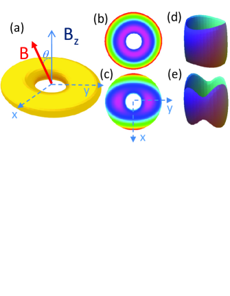
Figure 1: (a) Magnetic field orientation and coordinate system. Potential profile maps for (b) the circularly symmetric and (c) the elliptically deformed ring; purple regions show lowest energy values of the confinement potential. Electronic orbital for an excited state of an elliptical ring ($\delta=2$ meV), in the presence of a Rashba field ($F=100$ kV/cm) in a magnetic field ($B=2.375$ T) at different tilt angles, (d) $\theta=0^{\circ}$ and (e) $\theta=60^{\circ}$.

II.1 Tilted Magnetic Field

In the presence of a magnetic field $\vec{B}=\hat{x}B_{x}+\hat{z}B_{z}=\hat{x}B\sin\theta+\hat{z}B\cos\theta$, the vector potential can be written as

$$\vec{A}=\frac{B_{z}}{2}\rho\hat{\varphi}-B_{x}{z}\left(\hat{\rho}\sin\varphi+\hat{\varphi}\cos\varphi\right)\,.$$ (5)

It is important to note that small variations of the magnetic field angle $\theta$ induce considerable changes in the electronic structure, as the tilted magnetic field and ring asymmetry ($\delta\neq 0$) couples angular and radial degrees of freedom. In the absence of SOC, the system is described by the Hamiltonian,

$$\emph{H}=\frac{1}{2\mu^{*}}\left(\vec{p}-e\vec{A}\right)^{2}+V(\vec{r})+\frac{1}{2}g\mu_{B}\vec{B}\cdot\vec{\sigma}\,,$$ (6)

where the third term is the Zeeman interaction and $\vec{\sigma}=(\sigma_{x},\sigma_{y},\sigma_{z})$ are the Pauli matrices. Eq. (6) can be separated into three parts, $\emph{H}=H_{B_{z}}+H_{B_{x}}+H_{Z_{x}}$. The contribution due to the perpendicular component of the magnetic field ($B_{z}$) is given by

$$H_{B_{z}} = -\frac{\hbar^{2}}{2\mu^{*}}\left[\frac{1}{\rho}\frac{\partial}{\partial\rho}\left(\rho\frac{\partial}{\partial\rho}\right)+\frac{1}{\rho^{2}}\frac{\partial^{2}}{\partial\varphi^{2}}+\frac{\partial^{2}}{\partial{z^{2}}}\right]$$

$$+ \frac{ie\hbar{B_{z}}}{2\mu^{*}}\frac{\partial}{\partial\varphi}+\frac{e^{2}B_{z}^{2}\rho^{2}}{8\mu^{*}}+V(\vec{r})$$

$$+ \frac{g\mu_{B}}{2}B_{z}\sigma_{z}\,.$$

The eigenfunctions of the circularly symmetric problem ($\delta=0$) in the presence of the $B_{z}$ component, $\Phi_{lmn}(z,\rho,\varphi)$, are used as the basis set to expand the eigenstates for a general tilted field direction, under SOC, and a general elliptical deformation. A general wavefunction can be written as

$$\Psi = \sum_{l,m,n}\left(C_{lmn}^{\uparrow}\mid\uparrow\rangle+C_{lmn}^{\downarrow}\mid\downarrow\rangle\right)\Phi_{lmn}\,,$$ (8)

where the spatial dependence has been omitted for simplicity. The term due to the in-plane component of the magnetic field is

$$H_{B_{x}} = -\frac{ie\hbar{z}B_{x}}{\mu^{*}}\left(\sin\varphi\frac{\partial}{\partial\rho}+\frac{\cos\varphi}{\rho}\frac{\partial}{\partial\varphi}\right)$$ (9)

$$+ \frac{e^{2}}{2\mu^{*}}\left(B_{x}^{2}z^{2}-B_{z}B_{x}z\rho\cos\varphi\right)\,.$$

and the respective Zeeman contribution can be written aszeemansplitting

$$H_{Z_{x}}=\frac{1}{4}g\mu_{B}B_{x}(\sigma^{+}+\sigma^{-})\,,$$ (10)

where $\sigma^{\pm}=\sigma_{x}\pm i\sigma_{y}$.

II.2 Spin-Orbit Coupling

The presence of spin-orbit coupling in the host semiconductor is also considered for the tilted magnetic field case. The SOC in the presence of system inversion asymmetry can be written in terms of the field associated with the confinement potential, $\nabla V(\textbf{r})$, as 3

$$H_{SIA}=\frac{\alpha_{s}}{\hbar}\vec{\sigma}\cdot\left(\nabla V\times(\vec{p}-e\vec{A})\right)\,,$$ (11)

where $\alpha_{s}$ characterizes the strength of the SOC in the host semiconductor. This can be decomposed in cylindrical coordinates into four terms, $H_{SIA}$=$H_{SIA}^{D}+H_{R}+H_{K}+H^{TF}_{SIA}$, where 3

$$H_{SIA}^{D} = \alpha_{s}\sigma_{z}\left\{\frac{\partial{V}}{\partial\rho}\left[-\frac{i}{\rho}\frac{\partial}{\partial\varphi}+\frac{eB_{z}}{2\hbar}\rho\right]+\frac{i}{\rho}\frac{\partial{V}}{\partial\varphi}\frac{\partial}{\partial\rho}\right.$$ (12)

$$+ \left.\frac{i}{\rho^{2}}\frac{\partial{V}}{\partial\varphi}\right\}\,,$$

$$H_{R} = -\alpha_{s}\frac{\partial{V}}{\partial{z}}\left\{\sigma^{+}\left[e^{-i\varphi}\left(\frac{\partial}{\partial\rho}-\frac{i}{\rho}\frac{\partial}{\partial\varphi}+\frac{eB_{z}}{2\hbar}\rho+\frac{1}{\rho}\right)\right]\right.$$ (13)

$$- \left.\sigma^{-}\left[e^{i\varphi}\left(\frac{\partial}{\partial\rho}+\frac{i}{\rho}\frac{\partial}{\partial\varphi}-\frac{eB_{z}}{2\hbar}\rho+\frac{1}{\rho}\right)\right]\right\}\,,$$

and $H_{K}=0$ because $\langle{k_{z}}\rangle\simeq 0$. $H_{SIA}^{D}$ is the spin-diagonal contribution due to the confinement, while the Rashba term $H_{R}$ is associated with the perpendicular electric field in the well, $\partial V/\partial z=eF$. For a tilted magnetic field, the last term in $H_{SIA}$ is given by

$$H_{SIA}^{TF} = \alpha_{s}\frac{ezB_{x}}{\hbar}\left(\frac{\partial{V}}{\partial{z}}\sigma_{x}-\frac{\partial{V}}{\partial{x}}\sigma_{z}\right).$$ (14)

The SOC mixes states depending on their spin component, following effective “selection rules” that select specific angular momentum quantum numbers according to the corresponding interaction term. 3 As a consequence, the spin and angular momentum content of each state become hybrids or mixtures that change with field orientation and magnitude. For large magnetic fields, the Zeeman energy dominates and eventually polarizes spins along $\vec{B}$. Mixing is of course more noticeable near spectrum degeneracies, as we will see below.

II.3 Spin Content and Berry Phase

We characterize the spin content of different eigenstates by analyzing the expectation value for the different components. In particular, we define the spin projection respect to the $z$-axis, $\theta_{s}$, in terms of projections along and perpendicular to the plane,

$$\langle\sigma^{+}\rangle = \sum_{j}{C_{j}^{\uparrow*}C_{j}^{\downarrow}}\,,$$

$$\langle\sigma_{z}\rangle = \sum_{j}\left(|C_{j}^{\uparrow}|^{2}-|C_{j}^{\downarrow}|^{2}\right)\,$$ (15)

(where $j=\{n,l,m\}$ in all sums), so that

$$\theta_{s}=\arctan\frac{\langle\sigma_{z}\rangle}{\langle\sigma^{+}\rangle}+\frac{\pi}{2}\left(1-{\rm sgn}\langle\sigma^{+}\rangle\right)\,.$$ (16)

We also explore the spatial variation in the spin orientation (‘spin texture’) for each state, which is related to the vector spin density, whose components are given by

$$S_{x}(\vec{r}) = \sum_{j,j^{\prime}}\Phi_{j^{\prime}}^{*}(\vec{r})\left(C_{j^{\prime}}^{\uparrow*}C_{j}^{\downarrow}+C_{j^{\prime}}^{\downarrow*}C_{j}^{\uparrow}\right)\Phi_{j}(\vec{r})$$

$$S_{y}(\vec{r}) = -i\sum_{j,j^{\prime}}\Phi_{j^{\prime}}^{*}(\vec{r})\left(C_{j^{\prime}}^{\uparrow*}C_{j}^{\downarrow}-C_{j^{\prime}}^{\downarrow*}C_{j}^{\uparrow}\right)\Phi_{j}(\vec{r})$$

$$S_{z}(\vec{r}) = \sum_{j,j^{\prime}}\Phi_{j^{\prime}}^{*}(\vec{r})\left(C_{j^{\prime}}^{\uparrow*}C_{j}^{\uparrow}-C_{j^{\prime}}^{\downarrow*}C_{j}^{\downarrow}\right)\Phi_{j}(\vec{r})\,.$$ (17)

The Berry phase is an interesting quantity that characterizes the different eigenstates, especially as it incorporates the effects of external and SOC fields, and the influence of geometrical confinement. The Berry phase of a given eigenstate $\alpha$ is defined as XiaoRMP

$$\Theta_{\alpha}=i\int_{0}^{2\pi}\langle{\Psi_{\alpha}|\frac{\partial}{\partial{\hat{\varphi}}}|\Psi_{\alpha}\rangle}\,d\hat{\varphi}\,,$$ (18)

where $\hat{\varphi}$ parametrizes a cyclic adiabatic process; we consider here a closed path around the ring, so that $\Psi_{\alpha}(\varphi)\rightarrow\Psi_{\alpha}(\varphi+\hat{\varphi})$. Different experiments would probe the Berry phases in different fashion, depending on the measurement design. Transport phase measurements, for example, would result in a mostly additive contribution of various channels involved in the conductance signal, i.e., those close to the Fermi energy. We illustrate the effect of cumulative phase by considering the total Berry phase for a collection of states, defined over a certain ‘occupation’ in the ring (defined once such structure is connected to current reservoirs and a bias window is defined).

III Results

The calculation of the spectrum in the ring utilizes the full diagonalization of the Hamiltonian written in the basis that considers a sufficiently large Hilbert space, truncated to the desired accuracy. We typically consider 11 eigenstates, with angular momentum $|m|<5$ for each spin orientation. These are found sufficient for convergence in the entire field and parameter range considered in this work. 2

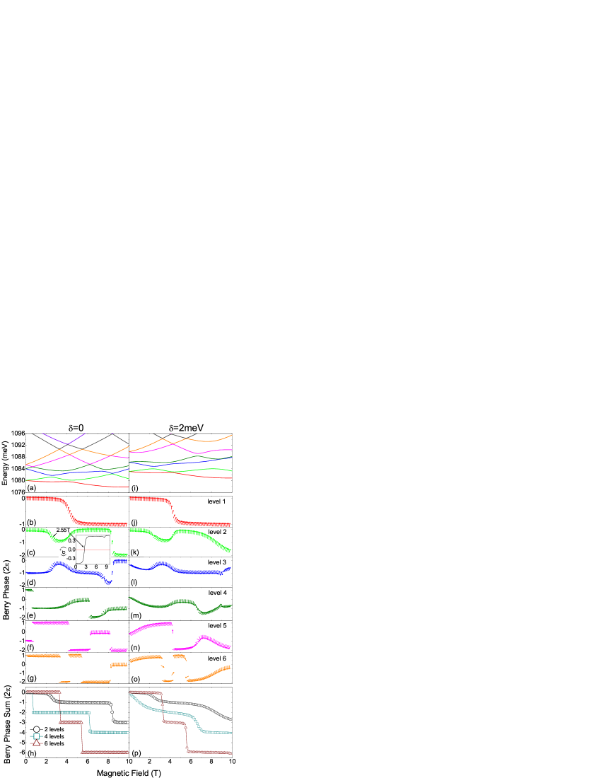
Figure 2: Electronic structure for quantum rings in a magnetic field at fixed tilt angle, $\theta=60^{\circ}$, and Rashba field $F=100$ kV/cm, as a function of the total magnetic field strength for: (a) symmetric ($\delta=0$) and (i) asymmetric ($\delta=2$ meV) ring. The Berry phase for different levels for $\delta=0$ is shown in panels on the left column, (b) through (g); and for $\delta=2$ meV on the right column, (j) through (o). The cumulative Berry phase for different occupation numbers is shown in panel (h) for the symmetric ring, and panel (p) for the asymmetric ring.

In what follows, we will assume parameters corresponding to InAs, with electron effective mass $\mu^{*}=0.0229m_{0}$, Landé g-factor $g=-14.9$, and SOC parameter, $\alpha_{s}=117.1$ Ų, taken from the literature. Winkler

Figures 2 and 3 show the electronic structure and the Berry phases for the lower energy manifold in both symmetric and asymmetric rings. In Fig. 2 we plot the energy levels and corresponding phases as function of the total magnetic field amplitude at a fixed angle, $\theta=60^{\circ}$, while Fig. 3 shows results for a fixed intensity of the magnetic field, $B=6.625$ T, as a function of the orientation $\theta$. The Berry phases of the lowest six levels are displayed in the figures 2 and 3, along with the corresponding mean spin orientations. The arrows along the different Berry phase curves indicate the spin orientation, with $\theta_{s}$ as defined above: An upwards/downwards arrow in these curves, $\theta_{s}=\pm\pi/2$, indicates a spin aligned along the $\pm z$-axis, while a horizontal arrow indicates a spin lying on the $x$-$y$ plane.

The results on the left panels of both figures are for a circularly symmetric quantum ring. For small magnetic field, the two lowest energy states exhibit spin alignment along $\pm z$-axis, as shown in Fig. 2(b) and (c). On the other hand, the next four levels (Fig. 2(d)-(g)) are aligned mostly on the plane due to the spin mixing caused by SOC. Notice that at high values of magnetic field levels become essentially aligned with (Fig. 2(b)-(d)) or against (Fig. 2(e)-(g)) the magnetic field, as the Zeeman energy dominates over the SOC. The evolution of spin orientation for each level is strongly influenced by the anticrossings with other levels, as one would expect. Moreover, anticrossings also affect the Berry phase of states, causing a smooth variation with large amplitude ($\simeq 2\pi$) in many cases, such as in Fig. 2(b) and (c) at around 4T; in Fig. 2(c) and (d) at around 2.5T, 4T and 8T; and at around 7.8T in 2(d) and (e).

Stronger spin-tilting and occasional total flips appear close to the region of nonzero (or $\neq 2\pi n$, with integer $n$) Berry phase, as shown in Fig. 2(c) at around 2.5T, and in 2(d) and (e) at around 7.8T. Thus, the spin hybridization and phase modulation are intrinsically linked due to SOC and magnetic field. Spin orientation and phase values smoothly change as a function of magnetic field intensity (or magnetic field orientation in Fig. 3). Some apparently sudden spin-flips also appear, as the one highlighted in panel 2(c), corresponding to a steep (yet continuous) variation of the spin component, as detailed in the inset. Similar smooth variations are presented for an eccentric (elliptically deformed) ring on the right panels, Fig. 2(j)-(o). The main effect introduced by the confinement asymmetry is to make the spin modulation and Berry phase vary more gradually with field intensity. This can be understood as arising from the asymmetry which introduces mixing of different angular momentum components and associated anticrossings. Notice in Fig. 2(i), that at higher magnetic fields, B$>$6T, various levels mix. This can be seen in the large anticrossings between levels 2 and 3 at around 7T, levels 4 and 5 at around 6.7T, and levels 5 and 6 at around 8.5T. The level mixture makes the spectrum flatter with field and, correspondingly, produces weaker variations in the Berry phase as well.

Figure 2(h) displays the gradual cumulative process of adding Berry phases of the first 2, 4, and 6 consecutive levels of panels (b)-(g). A similar addition has been obtained for the asymmetric ring case, shown in Fig. 2(p). This additive process is equivalent to increasing electron number or window around the Fermi level in a transport experiment). The cumulative Berry phase, especially for large number ($\gtrsim 3$) of levels counted is essentially null (or $=2\pi n$). In fact, although individual levels show strong variation of the Berry phase with field, the cumulative phase does not: successive levels have compensating Berry phase changes, so that the cumulative effect is surprisingly near null (except for occasional $2\pi$ slips shown in the figure), especially for the 4 and 6-level traces shown.

The introduction of quantum ring eccentricity changes the situation in a somewhat subtle fashion. Comparing left (h) and right (p) panels in Fig. 2, it is clear that as the eccentricity induces changes in the electronic spectrum and single-state Berry phases, the cumulative Berry phase shows gradual modulation, so that nontrivial values are seen over finite-size windows in field: 2 - 3T and 7 - 9T for cumulative Berry phase of 2 levels; 0 - 1T and 6 - 7T, for 4 levels; and 3 - 4T and 5 - 6T, for 6 levels. This would suggest that a moderate degree of asymmetry and/or disorder unavoidably present in real systems may in fact produce a more robust Berry phase signal in experiments.

Similar contrasts exist between circularly symmetric and asymmetric rings as function of magnetic field orientation (at constant strength), as shown in Fig. 3. As in Fig. 2, each state shows a gradual Berry phase evolution with magnetic field angle near level anticrossings, and the diamagnetic shift provided by $B_{z}$ decreases for larger angles. One can also see a rather interesting evolution of the spin orientation as the tilt angle increases. On the left panels, for the circularly symmetric ring, one also notices relatively sharp changes in Berry phase and spin orientation, as different angular momentum components are mixed by spin orbit coupling. Those jumps or drastic changes disappear or become smoother for the asymmetric ring (right panels), as the eccentricity mixes more strongly the different angular momentum states. Panels (h) and (p) show the cumulative Berry phase for the two rings. There is a similar behavior already seen in Fig. 2: a smooth variation with angle for small number of levels, changes to essentially null phase value ($2\pi n$) for larger level number. The sudden phase slips however become smoother, resulting in nontrivial values for the asymmetric ring over wider range (angular in this case).

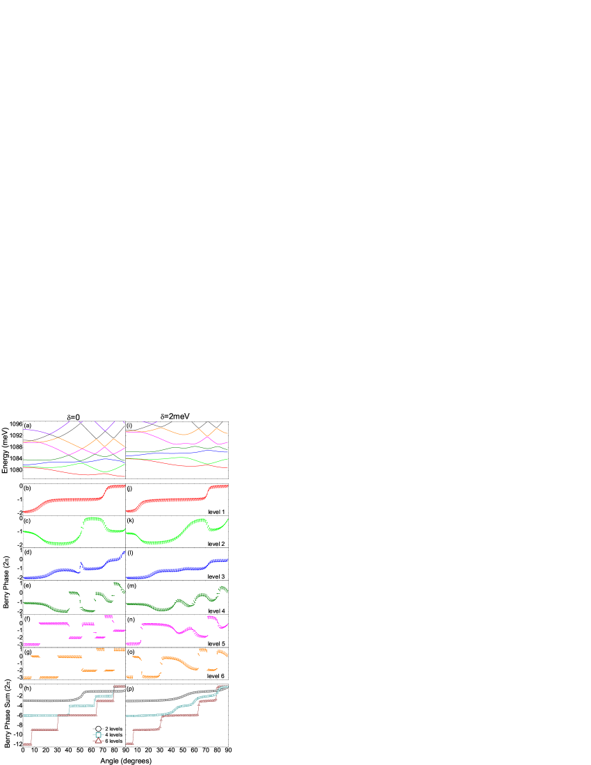
Figure 3: Electronic structure for quantum rings under fixed magnetic and Rashba fields, $B=6.625$ T and $F=100$ kV/cm, as a function of the magnetic field tilt angle $\theta$ for: (a) symmetric ($\delta=0$) and (i) asymmetric ($\delta=2$ meV) ring. Berry phases for different states in both rings are shown in the panels below. The cumulative Berry phase for different occupations is shown in panels (h) and (p), for the symmetric and asymmetric rings, respectively.

The slow evolution of Berry phase for each state signals the mixtures introduced by the different perturbations on an otherwise highly-symmetric picture. The Zeeman field, SOC, and structural asymmetries produce simultaneous mixtures of spin, parity, and angular momentum. This effect, contained in the expansion coefficients of the different states, can be visualized as well through spin density maps. Figure 4, left panels, show the expansion coefficients for the four lowest energy states of an asymmetric ring, as function of magnetic field, at a fixed angle $\theta=60^{\circ}$. These panels show solid (dashed) curves for the spin up (down) components with different angular momentum $m$ in the given state. The states are mixtures of angular momentum (introduced at zero field by the ring asymmetry) and/or spin (due to SOC), which evolve with field to other components (due to the diamagnetic shift of the spectrum), and eventually to more complex mixtures at higher energies.

The right panels in Fig. 4 show spin vector maps for the corresponding state at the field $B=2.375$T, and $\theta=60^{\circ}$. This field value corresponds to the anticrossing between the second and third levels in Fig. 2(i). The vector maps use arrows with size proportional to the spin density at each point on the plane (integrating each expression in Eq. (15) on the $z$-coordinate) and blue (or red) colors to indicate a positive (or negative) sign of the $z$-spin component at that point. The ground state (level 1) shows a spin map predominantly on the plane, although with overall positive $S_{z}$ component, and with high amplitude near the ends of the long-axis ellipse. The first-excited state, in contrast, shows large negative $S_{z}$ components and with a spatial distribution that complements that of the ground state. One also notices that the ground state spin map shows local vectors that are essentially parallel all along the ring: this would result in a vanishing Berry phase, as it is indeed seen in Fig. 2(j), at this magnetic field. For the second level, however, where the Berry phase $\simeq-\pi$ in Fig. 2(k), one notices that the spin arrows in Fig. 4 are canted with respect to those a quarter of the way along the ring. It is this non-parallel nature of the spins along the ring structure that characterizes a non-vanishing Berry phase. Levels 3 and 4 show even more structure, with spin vector amplitude more localized near the long ends of the ellipse, but with $S_{z}$ component that changes sign as one moves along the ring. The relative twisting of the spin vector density along the ring, contributes to the non-vanishing Berry phase seen in Fig. 2(l)-(m), although with much smaller value than for level 2. Other levels with non-vanishing Berry phase show similar canted spin texture across the ring.

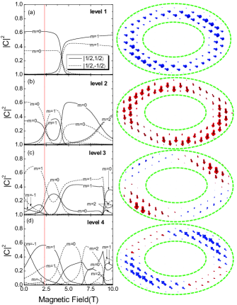
Figure 4: Panels on the left column shown expansion coefficients for the four lowest states of an asymmetric ring ($\delta=2$ meV), and fixed Rashba field $F=100$ kV/cm, and magnetic field tilt angle $\theta=60^{\circ}$, as function of magnetic field intensity. Level admixtures clearly evolve with sudden switches at level anticrossings. The right column shows spin density vector maps along the ring ($z$-integrated) for the four lowest states at a field $B=2.375$ T (indicated by the vertical line in left panels). Blue arrows have a positive projection along $z$, while for red arrows the projection is negative. Notice nearly parallel vectors in level 1 result in a null Berry phase; in contrast, canting of vectors in level 2 contribute to a Berry phase of $\simeq-\pi$ (see Fig. 2(k)).

IV Discussion and conclusions

We have used a nearly analytical description of the states in quantum rings of finite width. This model, used before to describe realistic structures in experiments, allows us to extract interesting insights on the role of spin-orbit coupling and its interplay with external magnetic field effects, such as diamagnetic shifts and Zeeman splitting. We have moreover introduced asymmetry in the confinement structure to see how this affects the level structure and associated spin texture and Berry phase of different states. We observed that possible experimental sweeps of magnetic field tilt or amplitude, produce controllable changes in the state characteristics, which can be traced in particular through the smooth variation of the Berry phase of each state. It is also clear that as spin-orbit coupling could be made stronger with applied electric fields, the Rashba effect would also controllably change the overall geometric phase in quantum rings.

Somewhat surprisingly, we found that the unavoidable defects or asymmetries in ring confinement produce smooth changes in the Berry phase, as either the magnetic field or tilt (or even Rashba field) is changed. This effect makes the otherwise sudden phase slips in symmetric rings become smoother and produce non-vanishing (or nontrivial) geometric phases as a consequence. This would suggest that moderate level mixing makes for more robust Berry phases in experiments. One should also comment, that although the multilevel cumulative Berry phase appears essentially null for higher level number (or wider energy window), it may be possible to access individual (or few) state Berry phases in narrow bias ranges or similar other experiments where few states can be sampled.

- (1) M. V. Berry, Proc. R. Soc. Lond. A 392, 45 (1984).
- (2) A. Shapere and F. Wilczek, Geometric Phases in Physics (World Scientific, Singapore, 1989).
- (3) D. Xiao, M.-C. Chang, and Q. Niu, Rev. Mod. Phys. 82, 1959 (2010).
- (4) Y. Aharonov and D. Bohm, Phys. Rev. 115, 485 (1959).
- (5) S. Filipp, J.Klepp, Y. Hasegawa, C. Plonka-Spehr, U. Schmidt, P. Geltenbort, and H. Rauch, Phys. Rev. Lett. 102, 030404 (2009).
- (6) A. G. Aronov and Y. B. Lyanda-Geller, Phys. Rev. Lett. 70, 343 (1993).
- (7) A. F. Morpurgo, J. P. Heida, T. M. Klapwijk, B. J. van Wees, and G. Borghs, Phys. Rev. Lett. 80, 1050 (1998).
- (8) J.B. Yau, E.P. De Poortere and M. Shayegan, Phys. Rev. Lett. 88, 146801 (2002).
- (9) T. Bergsten, T. Kobayashi, Y. Sekine, and J. Nitta, Phys. Rev. Lett. 97, 196803 (2006).
- (10) B. Grbić, R. Leturcq, T. Ihn, K. Ensslin, D. Reuter, and A. D. Wieck, Phys. Rev. Lett. 99, 176803 (2007).
- (11) F. Nagasawa, D. Frustaglia, H. Saarikoski, K. Richter, and J. Nitta, Nat. Commun. 4, 2526 (2013).
- (12) V. Lopes-Oliveira, Y. I. Mazur, L. D. Souza, L. A. B. Marçal, J. Wu, M. D. Teodoro, A. Malachias, V. G. Dorogan, M. Benamara, G. G. Tarasov, E. Marega Jr., G. E. Marques, Z. M. Wang, M. Orlita, G. J. Salamo, and V. Lopez-Richard, Phys. Rev. B 90, 125315 (2014).
- (13) M. D. Teodoro, A. Malachias, V. Lopes-Oliveira, D. F. Cesar, V. Lopez-Richard, G. E. Marques, E. Marega Jr., M. Benamara, Yu. I. Mazur and G. J. Salamo, J. Appl. Phys. 112, 014319 (2012).
- (14) G. Lommer, F. Malcher, and U. Rössler, Phys. Rev. Lett. 60, 728 (1988).
- (15) C. F. Destefani, S. E. Ulloa, and G. E. Marques, Phys. Rev. B 69, 125302 (2004).
- (16) R. Winkler, Spin-Orbit Coupling Effects in Two-Dimensional Electron and Hole Systems (Springer, Berlin, 2003).