Determining the filling factors of fractional quantum Hall states using knot theory

Abstract

In this work a method based on a topological invariance of rational tangles commonly used in knot theory determines filling factors in the fractional quantum Hall effect. The main sustain for this hypothesis are the Schubert’s theorems which treats the isotopic between two knots that are numerators of non-equivalent rational tangles. This isotopic allows to deduce a new formula for all filling factors. Besides, it opens a new perspective for a future connection between $N-$particles interaction at different fillings and Berry phase evaluated along torus knots.

I Introduction

The first sign for fractional Hall resistance was discovered by Tsui et al in 1982 Tsui et al. (1982); Stormer (1999). A high longitudinal conductivity was observed in GaAs-AlGaAs accompanied with a plateu in the Hall resistance within a filling factor of $1/3$. The number of filled Landau levels (LLs) characterises the filling factor as $\nu=\frac{\rho hc}{eB}$, where the electron density $\rho$, and magnetic field $B$, determine the Hall resistance as $R=\frac{h}{\nu e^{2}}$. One year later Laughlin published a $N-$particles wave function for the lowest Landau level (LLL) associated with fillings $1/q$ with $q-$odd Laughlin (1983). The comparison with numerical calculations showed Laughlin wave function was highly accurate, for a discussion see ref. Yoshioka (1985). Since the fraction $\nu$ is a dimensionless parameter one may attempt to define it as $\nu=p/q$ with $p$ and $q$ relatively primes. The case $q=1$ is known as the integer quantum Hall effect (IQHE). It was discovered by Klitzing in 1980 Klitzing et al. (1980). Its explanation consists in the interaction between an electron and the potential vector. The last is produced from the strong magnetic field applied perpendicular to a two dimensional (2D) sample where $N-$electrons remain confined at a very low temperature about 10mK Jain (2007); O. Heinonen (1998) (Ed). In contrast, the fractional quantum Hall effect (FQHE) which occurs at $q\neq 1$ is still partially understood. It is belived to be originated from the Coulomb interaction between electrons [Jain (2007), p.4]. A consistent description of the physical mechanism of FQHE ought to identify its buildding blokcs, explain incompressibility Jain (2014) and determine its state of matter at specific filling factor. One of the way to solve this enigma is by a construction of $N-$particles wave function. Thus it sHall be able to answer not only why the filling factors is a fractional number but to capture other fundamental feautures such as spin polarization and topological invariants. The last is the main topic of this paper. Furthermore an explanation of all Landau fillings with even denominator like the fraction $5/2$. The most popular hypothesis for solving this puzzle are wonderfull presented in Jain (2014). One of them is the composite fermions (CF) approach created by Jain Jain (1989). In this model the FQHE is produced by CF which are electrons within an even number of quantized fluxes. In CF theory the filling factor is

$$\nu=\frac{\nu^{*}}{2n\nu^{*}\pm 1}$$ (1)

with $n=0,1,2,3,...$ The trial wave function of CF at the LLL is $\psi_{\nu}=P_{LLL}\prod\limits_{i<j}^{N}(z_{i}-z_{j})^{2n}\phi_{\nu^{*}}$, where $\phi_{\nu^{*}}$ is the wave function of noninteracting electrons at integer filling $\nu^{*}=p$ Jain (2007). The idea behind this theoretical concept is that FQHE of electrons is created from an IQHE of CF. A successful comparison with experimental data and numerical calculations of the exact Coulomb energy Mukherjee et al. (2014); Jain (2014) has given to CF theory an extensive advantange over other models Kang et al. (1993). However certain fractions like $5/2$, $4/11$, $5/13$ do not fix into formula (1). In fact the fraction $5/13$ has been bautized as unconventional Mukherjee et al. (2014). Nevertheless they can be obtained with other expressions (Jain (2007), p. 207) than certainly are different than (1). The other good candidate to explore is the hierarchy theory of Halperin and Haldane (HH) Haldane (1983); Halperin (1984); Yoshioka (1985). In the HH hierarchy a daughter state generates Laughlin quasiparticles with fillings calculated from the continued fraction $\nu=[0,m,\pm q_{2},\pm q_{3},\pm q_{4},...,\pm q_{n}]$, where $m=3$ and $q_{n}=2$. The HH model is a hierarchy of fractions started from $1/m$. It reproduces all filling factors with odd denominators. The FQHE is explained by interplay of Laughlin quasiparticles at filling $1/m$ with fractional charge and fractional braid statistics. This braid statistics generates daughter states at filling $\nu$ Jain (2014). The physical assumptions behind CF and HH models arrange filling factors followed by a construction of wave fucntions of exotic particles with different charge and mass than electrons. Even a more amazing conclusion is that for a given filling factor corresponds a unique wave function. So, why $\nu$ is a exclusive parameter of the FQHE? The answer perhaps concerns with a relation between topology and quantum physics. In 80’s Thouless and Kohmoto Niu et al. (1985); Kohmoto (1985) have discovered that conductivity determines the integer filling connected with the winding number of a closed curved hooking a torus in a parameter space. This interpretation works nice for a topological description of the IQHE. For the FQHE, conductivity was produced by including degenaracy of the LLL. In 2006 Kohmoto et al Sato et al. (2006) had calculated the Kubo conductivity from ideas based on gauge invariance. The particle statistics was implemented from a braid group formalism on a torus. Although the CF and HH approahes are quite useful as a starting point for description of FQHE they still can not account in a unique way for wave functions at a filling with even denominator. In addition an explanation for the recent experimental results Dehghani and Mojaveri (2013); Willett (2013) in connection with the overabundance of filling factors in lower LLs relative to thouse with higher LLs. On the other hand it is known that statistics in 2D systems is rather anyons than only fermions or bosons since the fundamental group of the configuration space is isomorphic to the braid group $B_{n}$ Wu (1984). Progress in this area has been done within the cyclotron braid approach by Jacak et al in Jacak and Jacak (2014). A braid group called the cyclotron braid group with generators $b^{(n)}_{i}=\sigma^{n}_{i}$ has been introduced in references Jacak and Jacak (2010, 2011); J. Jacak, I. Jóźwiak, L. Jacak, K. Wieczorek (2011); J. Jacak, R. Gonczarek, L. Jacak, I. Jóźwiak (2012). This is an alternative framework founded in braid exchange and cyclotron orbits that describes the exotic statistics of CF allowing a braid interpretation of Laughlin correlations Jacak and Jacak (2010). The geometrical presentation of these braids are arcs with an odd number of crossings given by $k$. Filling factors reproduced thouse in (1) by the expression

$$\nu=\frac{p}{p(k-1)\pm 1}~{}.$$ (2)

In this paper we want to motivate an application of knot theory for a future construction of a quantum and topological description of CF’s. The main message from braids is a codification of anyon statistics by exchange of coordinates in the $N-$particles wave function Wilczek (1989); Wilczek, Frank (1990) (Ed). Therefore is is natural to introduce the very well known connection between braids and knots. For instance the Alexander’s theorem in Kunio Murasugi (1996) asserts that every closed braid is isotopic or in other words is topological equivalent to a knot. Therefore for every braid interpretation of CF there is an asociated knot description. In this work the richness of knot theory will be suitable for deduction of a formula from which is possible to obtain all filling fractions of CF including thouse with even denominator. The formula is deduced for a straightforward application of Schubert’s theorems for isotopic of knots numerators extracted from rational tangles R. L. Ricca (2001a) (Ed); Kauffman and Lambropoulou (2002, 2004). This theorem was originally formulated for closed braids named 4-plats Schubert (1954), (J. S. Birman (1974), pp. 212) or two bridge knots, see for instance ref. A. Kawauchi (1996); G. Burde (1985). The Schubert’s theorems for rational knots were analized by Kauffman et al in ref. Goldman and Kauffman (1997); Kauffman and Lambropoulou (2002, 2004). By following the structure of these theorems one may deduce that every filling factor is a topological invariant of rational tangles. This amazing fact is known as the Conway’s theorem mentioned in Kauffman and Lambropoulou (2002) and proven in ref. G. Burde (1985); Goldman and Kauffman (1997); Kauffman and Lambropoulou (2004). Rational tangles were introduced by Conway in 1967 within a geometrical presentation Conway (1967). Every rational tangle composed with two strands has a 3-braids representation Kauffman and Lambropoulou (2002, 2004). Additionally every rational knot has a 4-plat presentation and is formed by closing a tangle J. S. Birman (1974); G. Burde (1985); A. Kawauchi (1996); Goldman and Kauffman (1997). Moreover the theory of classical vortices has been formulated in terms of knots R. L. Ricca (2001a) (Ed); R. L. Ricca (2001b) (Ed). Some progress with quantum vortices such as thouse in superconductivity can be inflicted from a Chern-Simons theory Enger (1998); Lopez and Fradkin (1991); Zhang (1992); Kossow (2009). Amazingly path integrals of a Chern-Simons theory has explicitly shown the tipical skein relations of Jones polynomials which are invariants of knots Witten (1989, 2013); Bar-Natan (1995). The partition function defined from a Boltzmann factor has been used toghether with the Yang Baster equation to recovery Jones polinomials Wu (1992); Kunio Murasugi (1996). This connection can be profitable for characterization of topological properties of systems such as topological insulators Hasan and Kane (2010), distribution functions of 2D particle systems Lado (2003), FQHE in graphene J. Jacak, R. Gonczarek, L. Jacak, I. Jóźwiak (2012); Haldane (1988) and Wigner crystals Kivelson et al. (1986). In this work we will see that the Schubert’s theorems accomodate for a determination of filling factors for CF. The application is justified by the Conway’s theorem where filling factors can be taken as fractions that are topological invariants of rational tangles. Furthermore, the the Schubert’s theorems for rational knots, obtained as knot numerators of rational tangles, endure to establish a classification of filling factors of CF via isotopic of rational knots. Additionally an explanation of why filling factors with high numerator are rare can arise in knot theory from a relation between conductivity and Berry phase evaluated along torus knots R. L. Ricca (2001b) (Ed). Later the electric current is calculated by using a method based on a Laughlin’s idea explained in ref. Laughlin (1981). The result suggests an explanation of rare fillings due to innestabilities of the transformed potential energy caused by the Berry phase.

In Section II we begin with the definition of rational tangles and isotopy of knots. Besides a tangle method for filling fractions is described. In Section III the Schubert’s theorem for unoriented tangles determines a formula for filling factors of FQHE. The formula is generalized for the case of oriented tangles. In Section IV.1, a physical interpretation of a tangle is given in terms of conductivity. This interpretation is based on the fractional decomposition of the product of a rational winding number for torus knots and the Chern number. In Section V, a special case of planar isotopy is applied to the Hamiltonian. This isotopy transformation which is defined by a deformation of knots, yields a relation between the Coulomb energy and filling factors.

II Rational Tangles

Tangles were introduced originally by Conway in 1967 with the purpose of classifying alternating knots. A tangle is defined as a portion of a knot diagram from which there emerges just 4 arcs pointing in its compass direction Conway (1967). Examples of how tangles look like can be seen in ref. Conway (1967); Kauffman and Lambropoulou (2004). A special case of tangles are rational tangles which do not contain separated loops but only alternatings twist of two strands. An extension of these definition to arbitrary number of strands is likewise possible. A more formal definition of tangles in terms of homeomorphism is given by Kauffman and Lambropoulou in ref. Kauffman and Lambropoulou (2004). It is well known in knot theory Kauffman and Lambropoulou (2002); Kunio Murasugi (1996); G. Burde (1985); A. Kawauchi (1996); M. Watkins (1990) that a topological invariant of a rational tangle $T$ is a fraction denoted as F(T). Every fraction defined with relatively primes numbers can be decomposed in a continued fraction Olds (1963); G. Burde (1985) defined by the expression

$$F[T] = [a_{1},a_{2},a_{3},...,a_{m}]$$ (3)

$$= a_{1}+\cfrac{1}{a_{2}+\cfrac{1}{a_{3}+\cfrac{1}{..+\cfrac{1}{a_{k}}}}}$$

if $k$ is odd and either all $a_{i}>0$ or $a_{i}<0$ we say the fraction is written in a canonical form Kauffman and Lambropoulou (2002, 2004). For $k$-even it is easy to transform the fraction in a canonical form since $[a_{1},a_{2},a_{3},...,a_{k}]=[a_{1},a_{2},a_{3},...,a_{k}-1,1]$. In fact every continued fraction can be transformed to a unique canonical form. The associated tangle in statndard form Conway (1967); Kauffman and Lambropoulou (2002) is defined as

$$T = [[a_{1}],[a_{2}],[a_{3}],...,[a_{m}]]$$

$$= \biggl{(}\Bigl{(}([a_{m}]_{o}+[a_{m-1}])_{o}+...+[a_{3}]\Bigl{)}_{o}+[a_{2}]\biggl{)}_{o}+[a_{1}]$$

within a topological invariant given by (3) with properties

$$a. F(T+[\pm 1])=F(T)+1~{},$$ (5a)

$$b. F\Bigl{(}\frac{1}{T}\Bigl{)}=\frac{1}{F(T)}~{}.$$ (5b)

$$c. F(-T)=-F(T)~{}.$$ (5c)

A soft way to understand this definition is using a diagramatical reresentation of tangles. One may start knowing that all tangle diagrams are composed of the fundamental structures as in Fig. 1.

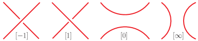
Figure 1: All tangles are composed of these elementary tangles Conway (1967).

The sum of two tangles $a+b$ is illustrated in Fig. 2. A reflexion $L_{o}$ in Fig. 3. and the inversion are defined by Fig. 4.

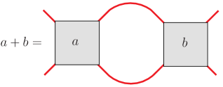
Figure 2: Sum of two tangles. Just join the adjacent arcs.

Figure 3: $L_{0}$ is the result of reflecting $L$ through its principal diagonal in the compass direction NW-SE Conway (1967). This introduce the Conway’s product for tangles as $ab=a_{0}+b$.

Figure 4: Inversion of a tangle Kauffman and Lambropoulou (2002, 2004). Rotating the tangle counterclock-wise by $90^{\circ}$ form a tangle $L^{r}$. The mirror image of a tangle is formed by switching all the crossings $-L=-(L)$. The inversion of a tangle is this rotation followed by its mirrow image.

Now a very important issue is the isoptopy of rational tangles Kauffman and Lambropoulou (2002); Kunio Murasugi (1996). It was established in 1975 as Theorem 1 (Conway): Two rational tangles are isotopic if and only if they have the same fraction. What it basically means is that a fraction is a topological invariant of rational tangles which are topological equivalent or in other words isotopic Conway (1967); Kauffman and Lambropoulou (2002); G. Burde (1985).

The Conway’s product of two tangles is a binary product defined as $ab=a_{o}+b$ Conway (1967). The Kauffman product $a*b$ Kauffman and Lambropoulou (2004) is as in Fig. 5

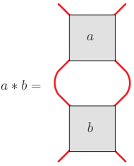
Figure 5: Kauffman product is a binary product. Moreover with this product the rational tangle in (II) can be as well defined Kauffman and Lambropoulou (2002).

II.1 Knot Numerator of a Rational Tangle

The connection between tangles and knots are acomplished by the closure of tangles as in Fig. 6.

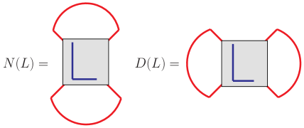
Figure 6: Knot numerator and denominator of a tangle $[L]$. We denote the numerator of a tangle $L$ as $N(L)$ and denominator as $D(L)$.

Here the knot numerator is a rational knot. Every rational knot is an alternating knot Kauffman and Lambropoulou (2002). The Schubert’s theorems deals with isotopy of knot numerators. Before going into this theorem we briefly review the idea of isotopy.

II.2 Concept of Isotopy

Isotopy between two knots means intuitively that a given knot can be deformed continuously into other by a surjective homotopy. Then one say the two knots are topological equivalent A. Kawauchi (1996); Kunio Murasugi (1996); G. Burde (1985). Therefore if two knots are isoptopic they define the same knot. Isotopy is formally express as: Let be $X$ and $Y$ two topological spaces and $f:X\to Y$ and $g:X\to Y$ homeomorphims. The functions f and g are isotopic and we denote $f\sim~{}g$ iff there exists a continuous surjective homotopy defined by the function $H(x,t)$ such that

$$H:X\times[0,1]\to Y$$ (6)

with $H(x,0)=f(x)$ and $H(x,1)=g(x)$.

There is an more efficient definition of isotopy for knots. It was originally proven the equivalence to the former in terms of Reidemeister moves Reidemeister (1927). More recent proofs in (ref. G. Burde (1985) p.1-9, 193), (ref. A. Kawauchi (1996) p.4, appendix A) (ref. Kunio Murasugi (1996) p.50, 13). The Reidemeister moves are transformations performed on parts of a knot. So take a knot and look for any of the configurations depicted in Fig. 7, then for that configuration it is allowed to do a Reidemeister move. There are three Reidemeister move described as following Kauffman (1990)

1. Twist and untwist a curl in either direction,

2. Lie down one loop completely over another,

3. A string can be moved over or under a crossing.

If two knots are related through a finite number of Reidemeister moves of type I, II, III they are said ambient isotopic Kunio Murasugi (1996); G. Burde (1985); Kauffman (1990). Similarly they are regular isotopic if one can be transformed into another by the moves of type II and III. Other definitions includes plane isotopy Web as deformations Kunio Murasugi (1996) such as rotation around a fix point, drag, translation and dilatation/elongation.

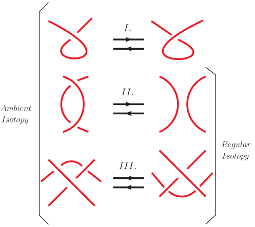
Figure 7: Reidemeister moves of type I, II and III. These moves can be performed in 2D on a regular diagram of a knot.

II.3 The Tangle Method

One may use tangles to classify the filling factors of FQHE. Let select a fraction in of FQHE, for intance $\frac{3}{11}$. It can be written as $[0,3,1,2]$ which is equals to a continued fraction in canonical form given by $[0,3,1,2-1,1]=[0,3,1,1,1]$. The tangle whose topological invariant is the fraction $\frac{3}{11}$ can be written in the standard form as $[[0],[3],[1],[2]]$. In order to find its knot numerator a presentation of the tangle is required. Following the expression (II) and the basic operations given in Fig. 1, Fig. 2, Fig. 3 one may find easily the result in Fig. 8.

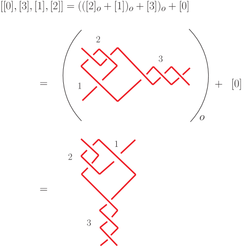
Figure 8: Presentation of a tangle with invariant fraction $\frac{3}{11}$. The knot numerator of this tangle is isotopic to the knot $3_{1}$.

The numerator closure of this tangle is isotopic to the knot $3_{1}$. Tables of knots up to twelve crossings can be consulted in the Rolsen table and the Hoste-Thistlethwaite table Atl . A full table of knots with twelve crossings can be seen in Tab . For more information, we address the reader with a didactical explanation in references Conway (1967); Kauffman and Lambropoulou (2002, 2004); Goldman and Kauffman (1997).

II.4 Recovery the Cyclotron Group

One may recovery the cyclotron braid group generators introduced in J. Jacak, R. Gonczarek, L. Jacak, I. Jóźwiak (2012) by using a $(N-1)-$Tangle. Therefore it is easy to see in Fig. 9 that if $k-$odd the tangle $[[0],[k]]=[k]_{o}+[0]$ is equals to $\sigma^{k}_{i}$.

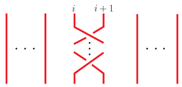
Figure 9: Presentation of the braid $\sigma^{k}_{i}$ with $i=1,2,3,...N-1$.

It gives exactly the generator $b^{(k)}_{i}$ introduced in reference (J. Jacak, R. Gonczarek, L. Jacak, I. Jóźwiak (2012), p.27-29).

II.5 Schubert’s Theorem for Unoriented knots

In this section is extressed that filling factors of FQHE are topological ivariants of rational tangles and can be organized by isotopy of rational knots. Here we present a theoretical support. The Schubert’s theorems for unoriented/oriented knots were introduced using 4-plats presentations of knots Schubert (1954); A. Kawauchi (1996); G. Burde (1985); J. S. Birman (1974). Developments with tangles are found in references Kauffman and Lambropoulou (2002, 2004); R. L. Ricca (2001b) (Ed). The first theorem is

Theorem 2 (Schubert): Suppose that rational tangles with fractions $\nu=\frac{p}{q}$ and $\nu^{\prime}=\frac{p^{\prime}}{q^{\prime}}$ are given ($p$ and $q$ are relatively prime. Similarly for $p^{\prime}$ and $q^{\prime}$.) If $N[\frac{p}{q}]$ and $N[\frac{p^{\prime}}{q^{\prime}}]$ denote the corresponding rational knots obtained by taking numerator closures of these tangles, then $N[\frac{p}{q}]$ and $N[\frac{p^{\prime}}{q^{\prime}}]$ are isotopic if and only if

1. $p=p^{\prime}$ and

2. either $q=\pm q^{\prime}+mp$ or $qq^{\prime}=\pm 1+mp$.

with m-integer. Since a knot is isotopic to itself one should take $m=1,2,3,...$

III A Formula for filling Factors in FQHE

The idea that filling factors are topological invariants was used in 1985 by Thoules et al Niu et al. (1985) via a calculation of conductivity. In this paper the Conway’s theorem is applied since it admits an interpretation of filling factors in FQHE as a topological invariants of rational tangles. A relation between tangles and conductivity will be appointed in Section IV.1.

The condition $p=p^{\prime}$ and $q=\pm q^{\prime}+mp$ of Thorem 2 is sumarized in the Kauffman’s equation Kauffman and Lambropoulou (2004)

$$(\pm T)*\frac{1}{[m]}=\frac{1}{[m]\pm\frac{1}{T}}~{}.$$ (7)

The equation (II) can be obtained inductively from (7). In any case if we define $F((\pm T)*\frac{1}{[m]})=\frac{p}{q}$ and $F[T]=\frac{p}{q^{\prime}}$ is easy to apply the propierties of (5a)-(5c) hence

$$F\left((\pm T)*\frac{1}{[m]}\right) = \frac{1}{m\pm\frac{1}{F(T)}}~{},$$ (8)

and then

$$\frac{p}{q} = \frac{p}{mp\pm q^{\prime}}~{}.$$ (9)

Certainly this result can be inferred directly from Schubert’s theorem. In terms of filling factors the formula (9) transforms in

$$\nu=\frac{\nu^{\prime}}{m\nu^{\prime}\pm 1}~{}.$$ (10)

This formula is presented including a formal concept of topological invariance and can be used to reproduce conventional filling factors in the FQHE. Notice that this theorem does not imposse restrictions on the integer $m$. Nevertheless it is effortless to see the Jain’s formula (1) is a special case of (10) when $m=2n$. The cyclotron formula (2) is the case when $m=k-1$. Additionally many filling factors of the HH theory are obtained by (10). At this point it is worth to mention that the fraction decomposition of the HH hierarchy is non-canonical since not all $a_{i}$ in (3) would have the same sign. One may remember that a canonical form of a fraction leads to rational tangles that are alternating. For instance, a canonical form of the fraction $\frac{4}{9}$ is $[0,2,4]$ which is the invariant of a rational tangle whose numerator clousure is the alternating link $L4a1$. In contrast, this fraction in the HH model is decomposed as $\frac{4}{9}=[0,3,2,-2,-2]$ yielding a no-rational tangle. Since in the HH theory the components of a continued fraction are fixed by the hierarchy there is not freedom to organize them via the isotopy of alternating knots.

III.1 Conventional versus Unconventional FQHE

The definition of unconventional fillings was introduced by Wójs et al in Mukherjee et al. (2014). Fractions which are out of expression (1) were defined as unconventional. Is there any topological reason for that? For instance, in Table 8 the invariants $\frac{7}{2}$, $\frac{7}{3}$, $\frac{7}{5}$ can not be obtained just by replacing in (10) the filling factor of IQHE given by $\nu^{\prime}=7$. So one may call them unconventional. A topological description can be constracted observing that the fraction $\frac{7}{2}$ is an invariant of the tangle $[[3],[2]]$ which has a knot numerator isotopic to $5_{2}$ which does not belong to the Table 1. In contrast $\frac{7}{13}$, $\frac{7}{15}$, $\frac{7}{27}$ are calculated using (10) having knot numerators as $7_{1}$. This is the same as the knot numerator of tangle with invariant $7$. This last fraction is associated to the seventh Landau level in the IQHE regime. Similarly in Table 6 the tangle whose invariant is the fraction $\frac{5}{11}$ has as a knot numerator $5_{1}$, the same as the knot numerator of the tangle with invariant $5$ which associates with the fifth Landau level in the IQHE. This is not the case of the tangle with invariant $\frac{5}{2}$ with knot numerator rather isotopic to $4_{1}$. As we may observe $4_{1}$ is not part of the invariants connected to the IQHE. Therefore in this context $\frac{5}{2}$ is unconventional as well and can not be obtained with formula (10). In topological terms, one may say that a filling factor for the FQHE is conventional if it is a topological invariant of a rational tangle with knot numerator isotopy to one of the IQHE. Otherwise is unconventional.

Consequently it would be convenient to construct a unique equation for conventional as well as unconventional fillings. Firstly let us notice that (7) and (10) do not bear enterely the second option impossed by Theorem 2. It is allow to have as well $qq^{\prime}=\pm 1+mp$. Therefore applying the full theorem 2 one obtain two options

$$\nu=\begin{cases}\frac{p}{mp\pm q^{\prime}}&\text{for ~{} $q^{\prime}=\pm~{}q^{\prime}+mp$}~{},\\ \frac{p}{\frac{m}{q^{\prime}}p\pm\frac{1}{q^{\prime}}}&\text{for ~{} $qq^{\prime}=\pm~{}1+mp$}~{}.\end{cases}$$ (11)

One may define $q=\alpha p~{}\pm~{}Q$ where either $\alpha=m$ and $Q=q^{\prime}$ or $\alpha=\frac{m}{q^{\prime}}$ and $Q=\frac{1}{q^{\prime}}$. Then both options in (11) can be written in a unique equation given by

$$\nu = \frac{p}{\alpha p~{}\pm~{}Q}~{}.$$ (12)

Where $p$ is the filling of the IQHE and $q^{\prime}$ might be interpreted as a parameter for the FQHE constrained to the former definitions. There are no obvious mathematical arguments which restrict the values of $p$ and $q^{\prime}$ but there could be physical reasons related with the dynamics of electrons. An attempt for a physical interpretation of filling factors in terms of rational tangles is given in the next section. Thus the Kauffman’s equation (7) would be

$$(\pm T)*\frac{1}{[\alpha]}=\frac{1}{[\alpha]\pm\frac{1}{T}}~{}.$$ (13)

where $[\alpha]$ is a rational tangle constrained to the rule (II). Additionally $\nu=F((\pm T)*\frac{1}{[\alpha]})$ and $F(T)=\frac{p}{Q}$. Now filling factors for the FQHE are organized via isotopy of knot numerators. The results are in Tables 1-11. Here below it is described briefly the procedure. For illustration take tangles connected with the IQHE region. Let it be $T=[1]$, with fraction $F(T)=1$ corresponding to the first LL. Therefore $p=1$, $Q=1$ and $\alpha=m$. This generates all fractions of the form

$$\frac{1}{q}=\Bigl{\{}1,\frac{1}{2},\frac{1}{3},\frac{1}{4},...\frac{1}{m\pm 1},...\Bigl{\}}~{}.$$ (14)

which are invariants of the tangles $[[0],[q]]$ with knot numerators isotopic to $0_{1}$. Successively $F(T)=2$ leads to

$$\frac{2}{q}=\Bigl{\{}2,\frac{2}{3},\frac{2}{5},\frac{2}{7},...\frac{2}{2m\pm 1},...\Bigl{\}}~{}.$$ (15)

with knot numerator isotopy to the link $L2a1$. $F(T)=3$ yields

$$\frac{3}{q}=\Bigl{\{}3,\frac{3}{2},\frac{3}{4},\frac{3}{5},...\frac{3}{3m\pm 1},...\Bigl{\}}~{}.$$ (16)

with knot numerator isotopy to the link $3_{1}$. $F(T)=4$ generates

$$\frac{4}{q}=\Bigl{\{}4,\frac{4}{3},\frac{4}{5},\frac{4}{7},...\frac{4}{4m\pm 1},...\Bigl{\}}~{}.$$ (17)

with knot numerator isotopy to the link $L4a1$. $F(T)=5$ leads to

$$\frac{5}{q}=\Bigl{\{}5,\frac{5}{4},\frac{5}{6},\frac{5}{9},...\frac{5}{5m\pm 1},...\Bigl{\}}~{}.$$ (18)

Amazingly the unconventional fillings as $\frac{5}{2}$, $\frac{5}{3}$, $\frac{5}{7}$, $\frac{5}{13}$ in Table 6 are associated to the knot $4_{1}$ which is not isotopic to any of the knot numerators for the IQHE. Hence one should have a new starting point with the filling factor of $F(T)=\frac{5}{2}$ and then $\alpha=\frac{m}{2}$, $Q=\frac{1}{2}$ yields

$$\Bigl{\{}\frac{5}{2},\frac{5}{3},\frac{5}{7},...\frac{10}{5m\pm 1},...\Bigl{\}}~{},$$ (19)

here $2q=5m\pm 1$ is an even number and so for unconventional fillings originated from $F(T)=\frac{5}{2}$ not all values of $m$ are allowed. Thus e.g. fillings like $\frac{10}{9},\frac{10}{11}$ do not belong to the same clasification since $5(2)-1=9$ and $5(2)+1=11$ are odd denominators.

Similarly there are unconventional fillings in Tables 8 and 10.

III.2 Shubert’s Theorem for Oriented Knots

Theorem 2 deals with isotopy of unoriented rational knots constructed from unoriented tangles. This theorem changes for the case of oriented knots. Furthermore if two tangles have different orientation their corresponding knot numerators might be distint even if the invariant fractions are the same. Therefore knots numerators must be built from compatible-oriented tangles. Two tangles are compatible-oriented if their end arcs have the same orientation. Notice that a tangle $[T]$ is orientation-compatible to $T*[2n]$ consequently $N(T)$ is isotopic to $N(T*[2n])~{}$ (Kauffman and Lambropoulou (2002), p. 45). The Theorem 3 elucidates a formula for invariants fillings of orientable tangles.

Theorem 3 (Schubert): Suppose that orientation-compatible rational tangles with fractions $\frac{p}{q}$ and $\frac{p^{\prime}}{q^{\prime}}$ are given ($p$ and $q$ are relatively prime. Similarly for $p^{\prime}$ and $q^{\prime}$.) If $N[\frac{p}{q}]$ and $N[\frac{p^{\prime}}{q^{\prime}}]$ denote the corresponding rational knots obtained by taking numerator closures of these tangles, then $N[\frac{p}{q}]$ and $N[\frac{p^{\prime}}{q^{\prime}}]$ are isotopic if and only if

1. $p=p^{\prime}$ and

2. either $q=\pm q^{\prime}+2np$ or $qq^{\prime}=\pm 1+2np$.

with n-integer. Thus a general formula for FQHE deduced on the base of Theorem 3 is

$$\nu=\frac{p}{2\alpha p\pm Q}~{},$$ (20)

with $q=2\alpha p~{}\pm~{}Q$ where either $\alpha=m$ and $Q=q^{\prime}$ or $\alpha=\frac{m}{q^{\prime}}$ and $Q=\frac{1}{q^{\prime}}$. In both cases the Kauffman’s equation for orientable tangles is

$$(\pm T)*\frac{1}{[2\alpha]}=\frac{1}{[2\alpha]\pm\frac{1}{T}}~{}.$$ (21)

where once more $[\alpha]$ is a rational tangle constrained to the rule (II). Let us take once again the tangle $T=[1]$ with fraction $F(T)=1$ corresponding to the LLL. This generates fractions of the form

$$\frac{1}{q}=\Bigl{\{}1,\frac{1}{3},\frac{1}{5},...\frac{1}{2m\pm 1},...\Bigl{\}}~{}.$$ (22)

just fillings with odd denominator. Nevertheless for $F(T)=\frac{1}{2}$, $p=1$, $\alpha=m$ and $Q=2$ is obtained the set

$$\Bigl{\{}\frac{1}{2},\frac{1}{4},...\frac{1}{2m\pm 2},...\Bigl{\}}~{}.$$ (23)

which are fractions with even denominator. However notice that $F(T)=\frac{1}{2}$ has not been generated from the LLL. This is a consequence of the orientation of knots numerators. Since the only difference between the knots numerators associated to (22) and (23) is the orientation then a knot numerator corresponding to a rational tangle with invariant filling factor of odd denominator has opposite orientation with respect to that of a filling of even denominator. The orientation of knots can be set experimentally by changing the orientation of the applied voltage applied to the 2D Hall system. This hypothesis might be related with the experimental anysotropy announced in ref. Lilly et al. (1999).

IV Where to find Knots in FQHE?

In this section we describe two canditates for knots in the FQHE. First: Impossing boundary conditions on a single particle wave function as it was done by Thouless et al in ref. Niu et al. (1985) yields a torus which determine a parameter space. For instance a set of lines on the 2D system would be seen as a knot on the torus surface. Torus knots have a rational winding number which is a basic ingredient of conductivity for the FQHE. See e.g section IV.1. Second: It is well known that a voltage must be applied to the 2D system in order to observe a current which experience a Hall resistance. One may naively imagine a 2-tangle created in time on a 2D sample by the transport of charge carries. The conductivity for such arrangment would be given by $\frac{e^{2}}{h}F(T)$. Equivalent definitions of conductivity in terms of tangles and knots were given in R. L. Ricca (2001a) (Ed); Goldman and Kauffman (1993).

IV.1 Conductivity

In this section we will examine the first candidate for a knot in the FQHE. The conductivity of a $N-$particles wave function for the FQHE is obtained by using the continued fraction approach for rational tangles in terms of the product of Chern and winding numbers. The last is associated to a torus knot living on the parameter space.

We start considering the average of the Hall conductivity for the N-particles ground state $\psi_{k}$ on a 2D square sample of length $L$ with FQHE. A unitary transformation given by $\phi_{k}=\exp\left[-i\frac{\theta}{L}(x_{1}+...+x_{N})\right]\exp\left[-i\frac{\varphi}{L}(y_{1}+...+y_{N})\right]\psi_{k}$ was employed by Thouless et al within the Kubo’s formula Niu et al. (1985). The result including the Berry phase $\gamma_{k}(\Gamma)$ is

$$\sigma = i\frac{e^{2}}{hd}\sum\limits^{d}_{k=1}\int\limits^{2\pi}_{0}\int\limits^{2\pi}_{0}\frac{d\theta\,d\varphi}{2\pi}\left[\left\langle\frac{\partial\phi_{k}}{\partial\theta}\Bigl{|}\frac{\partial\phi_{k}}{\partial\varphi}\right\rangle-\left\langle\frac{\partial\phi_{k}}{\partial\varphi}\Bigl{|}\frac{\partial\phi_{k}}{\partial\theta}\right\rangle\right]$$ (24)

$$= \frac{e^{2}}{hd}\sum\limits^{d}_{k=1}\int\limits^{2\pi}_{0}\int\limits^{2\pi}_{0}\frac{d\theta\,d\varphi}{2\pi}\left[\partial_{\theta}A_{\varphi}-\partial_{\varphi}A_{\theta}\right]$$

$$= \frac{e^{2}}{hd}\sum\limits^{d}_{k=1}\frac{\gamma_{k}(\Gamma)}{2\pi}~{}.$$

The parameters $\theta,\varphi$ are phases of a gauge transformation induced by magnetic translation operators acting on a single particle wave function, see ref. Niu et al. (1985). They define a 2D parameter space which can be mapped into a 2D torus due to the boundary conditions imposed on single particle wave functions. Here in this paper the closed curve on which the Berry phase is evaluated is taken as a torus knot living on the 2D torus. In a different approach but still using (24) Kohmoto et al employed the Kubo’s formula in the Brillouin zone Kohmoto (1985) within a periodic potential. More reciently the expression (24) was used with braid and gauge groups on a torus Sato et al. (2006).

A key point in the FQHE is the ground-state degeneracy counted by $d$. The index $k$ label degeneracy of the ground state. The relation between conductivity and the Berry phase is well known Huber and Lindner (2011); S. Huber (2013). For a closed curve $\Gamma$, enclosing the parameter space just once, the Berry phase vanishes modulo $2\pi$ J.J. Sakurai, J. Napolitano (1994) and the integer Chern number, $C_{k}$, determines the conductivity since the Berry phase is

$$\gamma_{k}(\Gamma) = \oint\limits_{\Gamma}A_{k}\left(R\right)\cdot dR$$ (25)

$$= 2\pi C_{k}~{},$$

and the Berry connection

$$A_{k}\left(R\right)=i~{}\langle\phi_{k}|\nabla_{R}|\phi_{k}\rangle~{}.$$ (26)

Here $\Gamma$ is a torus knot drawn by the two components dimensionless vector $R=(\theta,\varphi)$. Generally $R$ dependent on time and enters in the Hamiltonian (see e.g J.J. Sakurai, J. Napolitano (1994) pp. 349). Therefore here $\theta,\varphi$ vary with time and may be introduced in the Hamiltonian as a consequence of a gauge transformation Niu et al. (1985). This is a motivation to define a tangle using the conductivity from a Berry phase as the one in ref. S. Huber (2013); Niu et al. (1985). If the knot given by $\Gamma$ goes around the torus more than one time, the expression (24) is completed including the winding number L. Michel (2007) multiplied by the standard Berry phase J.J. Sakurai, J. Napolitano (1994). Then for the FQHE the equation (24) provides

$$\frac{1}{d}\sum\limits^{d}_{k=1}W_{k}C_{k}=F(T)~{}.$$ (27)

We remind by the Conway’s theorem that the filling factor $F(T)=\frac{p}{Q}$ defined in section III.1, is an invariant of a rationl tangle. For the IQHE when $F(T)=p$, all $W_{k}C_{k}$ must be equal and integers then degeneracy is unimportant since the sum disappear. Then the torus knot is given by $0_{1}$ which has a winding number equals one. For the FQHE the degeneracy of the ground state is relevant. One may define the total sum on degenerate states as $F(T)=WC$ which is the product of the rational winding number $W$ for torus knots and the integer Chern number $C$. In this sense the formula (27) which determines the conductivity in (24) would remains the same either for IQHE or FQHE. As we have mentioned the components of a rational tangle correspond to thouse of the continued fraction decomposition (3). Therefore the degree of degeneracy can be given by the number of components of the rational tangle. For instance, let us take the filling factor with four components as $\frac{3}{5}=[0,1,1,2]$ given in Table 4. If the degeneracy would be $8$ it is possible to expand the fraction to eight components as $[0,1,1,2]=[0,1,1,2,1,-1,1,-1]$. It is still possible if degeneracy is an odd number like $7$ then $[0,1,1,2]=[0,1,1,3,-1,1,-1]$. For an arbitrary closed curve the Euler algorithm G. Burde (1985), (Olds (1963), pp. 24) provides values for the Berry phase. Thus if a tangle associated to the ground state is $T=[[a_{1}],[a_{2}],[a_{3}],...[a_{k}],...[a_{d}]]$ with $a_{1}=0$ and $a_{k}\neq 0$. Then its invariant can be decomposed with the Euler algorithm as

$$F(T)=a_{1}+\sum\limits^{d}_{k>1}\frac{(-1)^{k}}{q_{k}q_{k-1}}$$ (28)

and so

$$\frac{\gamma_{1}}{2\pi} = da_{1}=0~{},$$ (29)

$$\frac{\gamma_{k>1}}{2\pi} = d\frac{(-1)^{k}}{q_{k}q_{k-1}}~{},$$ (30)

where

$$(-1)^{k} = p_{k}q_{k-1}-p_{k-1}q_{k}$$ (31)

$$p_{k} = a_{k}p_{k-1}+p_{k-2}~{},$$ (32)

$$q_{k} = a_{k}q_{k-1}+q_{k-2}~{},$$ (33)

within initial values

$$p_{0}=1 p_{-1}=0~{},$$ (34)

$$q_{0}=1 q_{-1}=1~{},$$ (35)

$$p_{d}=p q_{d}=Q~{}.$$ (36)

As a conclusion, from (29) is deduced that there might be an state in the LLL such that the Berry phase $\gamma_{1}=0$ and so the Berry curvature vanish J.J. Sakurai, J. Napolitano (1994). This state is associated to the tangle $[0]$, with fraction F(T)=0, which produces a perfect insulator with ultrahigh resistance. Of course this is an extreme case where the Euler algorithm breaks down since one would be obligated to do $a_{k}=0$ too. Moreover the Kubo’s formula given in (24) might be invalid and apply only for liquid like states with no vanishing fillings Niu et al. (1985). The Kauffman equation given by (8) is consistent with a description based on Kubo’s formula since it is forbidden to divide by the tangle $T=[0]$.

V Isotopy and Potential Energy

There is other way to obtain filling factors with torus knots. In this section it is shown that the Laughlin explanation for the IQHE in ref. Laughlin (1981) is generalized for the case of FQHE. A beautiful relation emerges when isotopy between torus knots is considered. Here the Berry connection is multiplied with the magnetic flux quantum $\phi_{0}=\frac{h}{2e}$ and added to the vector potential inside the N-particles Hamiltonian.

V.1 Case IQHE

The IQHE can be described by the $N-$electrons Hamiltonian

$$H=\sum\limits^{N}_{s=1}\frac{1}{2m_{b}}\left(p_{s}+\frac{e}{c}A(x_{s},y_{s})+\frac{e}{c}\frac{\phi_{0}L}{\sqrt{N}}A\right)^{2}~{}.$$ (37)

A similar approach has been performed with the help of fluxes in ref. Jain (2007) or a vector field in ref. Laughlin (1981). However here our vector field $A$ is the Berry connection associated with the non-degenerated ground state. Here $A(x_{s},y_{s})$ is the vector potential produced by the magnetic field perpendicular to a 2D square sample of length $L$. Furthermore the torus knot in the 2D parameter space is taken as the knot numerator of a rational tangle as $\Gamma={\bf N}(T)$ and so

$$\gamma(N(T)) = \oint\limits_{{\bf N}(T)}i~{}\langle\phi|\nabla_{R}|\phi\rangle\cdot dR~{},$$ (38)

Since the radious of the cyclotron orbit for the state $\phi$ depends on the magnetic field as $r_{s}\sim\frac{1}{B}$, it is expected that under an isotopy transformation on $N(T)$ the cyclotron orbit change. An isotopy is realized by setting a new constant value for the magnetic field $B^{\prime}$. This relates with the old as $B^{\prime}=\frac{B}{\delta}$. It is a dilatation for $\delta<1$ if the cyclotron radius is smaller than the previous value. It is a elongation for $\delta>1$ if a cyclotron radius is bigger than before. This isotopy is generally a deformation because of the change in the knot size. Therefore if the separation between two charge carries at a given time is $r_{s}=R-R^{\prime}$ then under a deformation it transforms as

$$r^{\prime}_{s}=\delta r_{s}~{},$$ (39)

therefore the new knot determined by the vector $R^{\prime}=\delta R$ is such that ${\bf N}(T^{\prime})=\delta{\bf N}(T)$. This deformation changes the value of the filling factor and the Berry phase hence

$$\gamma({\bf N}(T^{\prime})) = \oint\limits_{{\bf N}(T^{\prime})}i~{}\langle\phi|\nabla_{R^{\prime}}|\phi\rangle\cdot dR^{\prime}~{},$$ (40)

$$= \oint\limits_{\delta{\bf N}(T)}i~{}\langle\phi|\frac{1}{\delta}\nabla_{R}|\phi\rangle\cdot d(\delta R)~{},$$

$$= \oint\limits_{\delta{\bf N}(T)}i~{}\langle\phi|\nabla_{R}|\phi\rangle\cdot dR~{},$$

$$\neq \gamma({\bf N}(T))~{}.$$

and the Berry connection is deformed as

$$A^{\prime}=i~{}\langle\phi|\frac{1}{\delta}\nabla_{R}|\phi\rangle~{}.$$ (41)

As a result the N-particles Hamiltonian is deformed as

$$H^{\prime} = \sum\limits^{N}_{s=1}\frac{1}{2m_{b}}\left(p_{s}+\frac{e}{c}A(x_{s},y_{s})+\frac{e}{c}\frac{\phi_{0}L}{\sqrt{N}}A^{\prime}\right)^{2}~{},$$ (42)

this Hamiltonian induced a current operator Laughlin (1981); Oh (Contemporary Mathematics 512, Symplectic Topology and Measure Preserving Dynamical Systems 2006). The result of considering isotopy is

$$I=\frac{dH^{\prime}}{dA^{\prime}}=\sum\limits^{N}_{s=1}\frac{e\phi_{0}L}{c\sqrt{N}m_{b}}\left(p_{s}+\frac{e}{c}A(x_{s},y_{s})+\frac{e}{c}\frac{\phi_{0}L}{\sqrt{N}}A^{\prime}\right)~{}.$$ (43)

The average of (43) together with an integration along the knot yields

$$\frac{c^{2}m_{b}}{2\pi h(\phi_{0}L)^{2}}\oint\limits_{{\bf N}(T)}\langle\phi|I|\phi\rangle\cdot dR = \frac{e^{2}}{2\pi h}\oint\limits_{{\bf N}(T)}A^{\prime}\cdot dR~{},$$ (44)

$$= \frac{e^{2}}{h}\frac{\gamma({\bf N}(T))}{2\pi}~{},$$

$$= \mathbb{n}~{},$$

which corresponds to the filling factor for the IQHE.

V.2 Case FQHE

The Hamiltonian in the FQHE is

$${\bf H}=H+V$$ (45)

where $V=\sum\limits^{N}_{i,j=1}\frac{e^{2}}{|\mathbb{r}_{i}-\mathbb{r}_{j}|}$ is the potential energy. However the Berry connection for degenerated N-particles is $A_{k}$, so the index $k$ labels degenration of the ground state. Now let us define a new vector named $B_{k}$ such that the Berry connection obeys $A_{k}\cdot B_{k}=1$. If the 2D connection is $A_{k}=(a_{1},a_{2})$ then the new vector is given by $B_{k}=\frac{1}{2}(a^{-1}_{1},a^{-1}_{2})$. As a consequence the Berry connection is deformed as in (41) by the value

$$\delta=A_{k}\cdot B^{\prime}_{k}~{}.$$ (46)

Additionally notice that $(dA_{k})\cdot B_{k}+A_{k}\cdot dB_{k}=0$ and so

$$\frac{dB_{k}}{dA_{k}}=-\frac{1}{|A_{k}|^{2}}~{}.$$ (47)

Besides the Hamiltonian transformed after an isotopy deformation is

$${\bf H}^{\prime}=H^{\prime}+V^{\prime}~{},$$ (48)

where the new value for the potential energy is originated by the isotopy (39) as $V^{\prime}=\frac{V}{\delta}$. Similar as the procedure used to obtain (43), the current for the FQHE is then calculated from ${\bf I}=\frac{d{\bf H}^{\prime}}{dA^{\prime}_{k}}$ in the expression

$${\bf I} = I+\frac{dV^{\prime}}{dA^{\prime}_{k}}~{}.$$ (49)

The IQHE is recovered from (49) in the absence of isotopy. In other words, when $\delta=1$ and so $V^{\prime}$ would equal $V$ which is independent of $A^{\prime}_{k}$. Furthermore the degeneration of the ground state is introduced with the standard sum $\frac{1}{d}\sum\limits^{d}_{k=1}$. The average and integration of (49) yields the FQHE filling factor as

$$\frac{c^{2}m_{b}}{2\pi h(\phi_{0}L)^{2}}\frac{1}{d}\sum\limits^{d}_{k=1}\oint\limits_{{\bf N}(T^{\prime})}\langle\phi_{k}|{\bf I}|\phi_{k}\rangle\cdot dR=$$

$$\mathbb{n}+\frac{c^{2}m_{b}}{2\pi h(\phi_{0}L)^{2}}\frac{1}{d}\sum\limits^{d}_{k=1}\oint\limits_{{\bf N}(T^{\prime})}\langle\phi_{k}|\frac{dV^{\prime}}{dA^{\prime}_{k}}|\phi_{k}\rangle\cdot dR~{},$$ (50)

This gives the value for the filling factor of FQHE as

$$\nu=\frac{c^{2}m_{b}}{2\pi h(\phi_{0}L)^{2}}\frac{1}{d}\sum\limits^{d}_{k=1}\oint\limits_{{\bf N}(T^{\prime})}\langle\phi_{k}|{\bf I}|\phi_{k}\rangle\cdot dR~{},$$ (51)

where $\mathbb{n}$ is calculated from (44) and it is a topological invariant of the tangle $T$. On the other hand the filling factor $\nu$ is a topological invariant of the tangle $T^{\prime}$. It must be extressed that (V.2) can not be used as a relation between fillings factors of IQHE since knot numerators of IQHE are not isotopic, see Table 1. For unoriented or oriented knots the expression (51) equals the equations (12) and (20) repectively. For instance, as it was mentioned before, the value $p\to\infty$, in (12), is a superconductive state which for unoriented knot generates finite filling factors for the FQHE as

$$\nu=\frac{1}{\alpha}~{},$$ (52)

thus from (V.2) and (51) is obtain

$$\frac{c^{2}m_{b}}{2\pi h(\phi_{0}L)^{2}}\frac{1}{d}\sum\limits^{d}_{k=1}\oint\limits_{{\bf N}(T^{\prime})}\langle\phi_{k}|\frac{dV^{\prime}}{dA^{\prime}_{k}}|\phi_{k}\rangle\cdot dR=\frac{1}{\alpha}-\mathbb{n}~{},$$ (53)

Consequently the potential is stable for the value $\alpha=\frac{1}{\mathbb{n}}$. Let us consider now the case when $\mathbb{n}$ is finite. So large values of $\nu$ are produced by innestabilities in the potential $V^{\prime}$. Now the derivative inside (53) for $\delta\neq 1$ is calculated using (47) as follows

$$\frac{dV^{\prime}}{dA^{\prime}_{k}} = -\frac{V}{\delta^{2}}\frac{\partial\delta}{\partial A^{\prime}_{k}}=-\frac{V}{\delta^{2}}\frac{\partial(A_{k}\cdot B^{\prime}_{k})}{\partial A^{\prime}_{k}}=-\frac{V}{\delta^{2}}\left(A_{k}\frac{\partial B^{\prime}_{k}}{\partial A^{\prime}_{k}}\right)~{},$$ (54)

$$= \frac{V}{\delta^{2}}\frac{A_{k}}{|A^{\prime}_{k}|^{2}}=V\frac{A_{k}}{|A_{k}|^{2}}~{}.$$

Finally by replacing (54) in (53) a relation between filling factors and Coulomb potential arises as

$$\frac{c^{2}m_{b}}{2\pi h(\phi_{0}L)^{2}}\frac{1}{d}\sum\limits^{d}_{k=1}\langle\phi_{k}|V|\phi_{k}\rangle\oint\limits_{{\bf N}(T^{\prime})}\frac{A_{k}}{|A_{k}|^{2}}\cdot dR=\frac{1}{\alpha}-\mathbb{n}~{}.$$ (55)

*

Appendix A Filling Factors of FQHE with the Tangle Method

As we show in Fig. 5 the tangle method can be used to classify filling factors of FQHE. Each fraction is a topological invariant of a rational tangle. The Theorem 2 is used to organized these fractions according the isotopy of knot numerators. Thus using the method exemplified in Section II.3 one can get the tables Tables 2 - 11. In these tables the filling factors are confirmed by experimental results published in ref. Eisenstein et al. (2000); Pan et al. (2003)

Table 1: Filling factors for the IQHE. Notice that the knot numerators of tangles $[1]$ and $[\infty]$ are isotopic. Alternatings knots with more than ten crossings like $K11a364$ are denoted with letter K. Links start with letter L like $L2a1$ which is the Hopf-Link. The $0_{2}$ stays for two unknots.

$\nu$	0	1	2	3	4	5	6	7	p-odd	p-even	$\infty$
T	[0]	[1]	[2]	[3]	[4]	[5]	[6]	[7]	[p]	[p]	$[\infty]$
N(T)	$0_{2}$	$0_{1}$	$L2a1$	$3_{1}$	$L4a1$	$5_{1}$	L6a3	$7_{1}$	Knot	Link	$0_{1}$
D(T)	$0_{1}$	$0_{1}$	$0_{1}$	$0_{1}$	$0_{1}$	$0_{1}$	$0_{1}$	$0_{1}$	$0_{1}$	$0_{1}$	$0_{2}$

Table 2: Filling factors for the FQHE $\frac{1}{q}$. Notice that absolutely all knot numerators of tangles [[0],[q]] are isotopic to the knot $N([1])\sim 0_{1}$ which associates with the LLL of IQHE.

$\nu$	$\frac{1}{2}$	$\frac{1}{3}$	$\frac{1}{4}$	$\frac{1}{9}$	$\frac{1}{q}$ ($q-$odd)	$\frac{1}{q}$ ($q-$even)
T	$[[0],[2]]$	$[[0],[3]]$	$[[0],[4]]$	$[[0],[9]]$	$[[0],[q]]$	$[[0],[q]]$
N(T)	$0_{1}$	$0_{1}$	$0_{1}$	$0_{1}$	$0_{1}$	$0_{1}$
D(T)	$L2a1$	$3_{1}$	$L4a1$	$9_{1}$	Knot	Link

Table 3: Filling factors for $\frac{2}{q}$. All knot numerators of tangles [[0],[k],[2]] are isotopic to $N([2])\sim L2a1$.

$\nu$	$\frac{2}{3}$	$\frac{2}{5}$	$\frac{2}{7}$	$\frac{2}{2k+1}$ ($k=0,1,2,...$)
T	$[[0],[1],[2]]$	$[[0],[2],[2]]$	$[[0],[3],[2]]$	[[0],[k],[2]]
N(T)	$L2a1$	$L2a1$	$L2a1$	$L2a1$
D(T)	$3_{1}$	$4_{1}$	$5_{2}$	Knot

Table 4: Filling factors for $\frac{3}{q}$. Knot denominators have $k+2$ crossings. They are isotopy to $N([3])\sim 3_{1}$

$\nu$	$\frac{3}{2}$	$\frac{3}{4}$	$\frac{3}{5}$	$\frac{3}{7}$	$\frac{3}{8}$	$\frac{3}{11}$
T	$[[1],[2]]$	$[[0],[1],[3]]$	$[[0],[1],[1],[2]]$	$[[0],[2],[3]]$	$[[0],[2],[1],[2]]$	$[[0],[3],[1],[2]]$
N(T)	$3_{1}$	$3_{1}$	$3_{1}$	$3_{1}$	$3_{1}$	$3_{1}$
D(T)	$L2a1$	$L4a1$	$4_{1}$	$5_{2}$	$L5a1$	$6_{1}$

Table 5: Filling factors for $\frac{4}{q}$. Isotopy to $N([4])\sim 4_{1}$

$\nu$	$\frac{4}{3}$	$\frac{4}{5}$	$\frac{4}{7}$	$\frac{4}{9}$	$\frac{4}{11}$	$\frac{4}{15}$
T	$[[1],[3]]$	$[[0],[1],[4]]$	$[[0],[1],[1],[3]]$	$[[0],[2],[4]]$	$[[0],[2],[1],[3]]$	$[[0],[3],[1],[3]]$
N(T)	$L4a1$	$L4a1$	$L4a1$	$L4a1$	$L4a1$	$L4a1$
D(T)	$3_{1}$	$5_{1}$	$5_{2}$	$6_{1}$	$6_{2}$	$7_{4}$

Table 6: Filling factors for $\frac{5}{q}$. Since $4_{1}$ and $5_{1}$ are not isotopic one is forced to use the two options of the Theorem 2. For instance the fraction $\frac{5}{9}$ can be obtained with the first option while the fraction $\frac{5}{11}$ needs the second option. This is a sign of unconventionallity.

$\nu$	$\frac{5}{2}$	$\frac{5}{3}$	$\frac{5}{7}$	$\frac{5}{9}$	$\frac{5}{13}$	$\frac{5}{13}$	$\frac{5}{19}$
T	$[[2],[2]]$	$[[1],[1],[2]]$	$[[0],[1],[2],[2]]$	$[[0],[1],[1],[4]]$	$[[0],[2],[5]]$	$[[0],[2],[1],[1],[2]]$	$[[0],[3],[1],[4]]$
N(T)	$4_{1}$	$4_{1}$	$4_{1}$	$5_{1}$	$5_{1}$	$4_{1}$	$5_{1}$
D(T)	$L2a1$	$3_{1}$	$5_{2}$	$6_{1}$	$6_{2}$	$7_{4}$	$8_{4}$

Table 7: Filling factors for $\frac{6}{q}$.

$\nu$	$\frac{6}{11}$	$\frac{6}{13}$	$\frac{6}{23}$	$\frac{6}{25}$
T	$[[0],[1],[1],[5]]$	$[[0],[2],[6]]$	$[[0],[3],[1],[5]]$	$[[0],[4],[6]]$
N(T)	$L6a3$	$L6a3$	$L6a3$	$L6a3$
D(T)	$7_{2}$	$8_{1}$	$9_{5}$	$10_{3}$

Table 8: Filling factors for $\frac{7}{q}$. Since $5_{2}$ and $7_{1}$ are not isotopic. Therefore unconventionallity is present here.

$\nu$	$\frac{7}{2}$	$\frac{7}{3}$	$\frac{7}{5}$	$\frac{7}{11}$	$\frac{7}{13}$	$\frac{7}{15}$	$\frac{7}{27}$
T	$[[3],[2]]$	$[[2],[3]]$	$[[1],[2],[2]]$	$[[0],[1],[1],[1],[3]]$	$[[0],[1],[1],[6]]$	$[[0],[2],[7]]$	$[[0],[3],[1],[6]]$
N(T)	$5_{2}$	$5_{2}$	$5_{2}$	$5_{2}$	$7_{1}$	$7_{1}$	$7_{1}$
D(T)	$L2a1$	$3_{1}$	$4_{1}$	$6_{2}$	$8_{1}$	$9_{2}$	$10_{4}$

Table 9: Filling factors for $\frac{8}{q}$. Knots start with letter K like $K11a364$ which is a knot of eleven crossings. The Hoste-Thistlethwaite table for eleven crossings can be found in Atl .

$\nu$	$\frac{8}{15}$	$\frac{8}{17}$	$\frac{8}{31}$
T	$[[0],[1],[1],[7]]$	$[[0],[2],[8]]$	$[[0],[3],[1],[7]]$
N(T)	$L8a14$	$L8a14$	$L8a14$
D(T)	$9_{2}$	$L10a114$	$K11a364$

Table 10: Filling factors for $\frac{9}{q}$. Since $6_{1}$ and $9_{1}$ are not isotopic. Therefore unconventionallity is present here. $K12a$ denotes one of the alternating knots with twelve crossings Tab .

$\nu$	$\frac{9}{13}$	$\frac{9}{19}$	$\frac{9}{35}$
T	$[[0],[1],[2],[4]]$	$[[0],[2],[9]]$	$[[0],[3],[1],[8]]$
N(T)	$6_{1}$	$9_{1}$	$9_{1}$
D(T)	$7_{3}$	$K11a247$	$K12a$

Table 11: Filling factors for $\frac{10}{q}$. $K13a$ denotes alternating knots with thirteen crossings Tab .

$\nu$	$\frac{10}{21}$	$\frac{10}{19}$	$\frac{10}{39}$
T	$[[0],[2],[10]]$	$[[0],[1],[1],[9]]$	$[[0],[3],[1],[9]]$
N(T)	$10_{1}$	$10_{1}$	$10_{1}$
D(T)	$K12a$	$K11a247$	$K13a$

References

- Tsui et al. (1982) D. C. Tsui, H. L. Stormer, and A. C. Gossard, Phys. Rev. Lett. 48, 1559 (1982).
- Stormer (1999) H. L. Stormer, Rev. Mod. Phys. 71, 875 (1999).
- Laughlin (1983) R. B. Laughlin, Phys. Rev. Lett. 50, 1395 (1983).
- Yoshioka (1985) D. Yoshioka, Progress of Theoretical Physics Supplement 84, 97 (1985).
- Klitzing et al. (1980) K. V. Klitzing, G. Dorda, and M. Pepper, Phys. Rev. Lett. 45, 494 (1980).
- Jain (2007) J. K. Jain, Composite Fermions (Cambridge University Press, USA, New York, 2007).
- O. Heinonen (1998) (Ed) O. Heinonen (Ed), Composite Fermions. A Unified View of the Quantum Hall Regime (World Scientific Publishing Co. Pte. Ltd, Singapore, Fairer Road, 1998).
- Jain (2014) J. K. Jain, ArXiv e-prints (2014), eprint 1403.5415.
- Jain (1989) J. K. Jain, Phys. Rev. Lett. 63, 199 (1989).
- Mukherjee et al. (2014) S. Mukherjee, S. S. Mandal, Y.-H. Wu, A. Wójs, and J. K. Jain, Phys. Rev. Lett. 112, 016801 (2014).
- Kang et al. (1993) W. Kang, H. L. Stormer, L. N. Pfeiffer, K. W. Baldwin, and K. W. West, Phys. Rev. Lett. 71, 3850 (1993).
- Haldane (1983) F. D. M. Haldane, Phys. Rev. Lett. 51, 605 (1983).
- Halperin (1984) B. I. Halperin, Phys. Rev. Lett. 52, 1583 (1984).
- Niu et al. (1985) Q. Niu, D. J. Thouless, and Y.-S. Wu, Phys. Rev. B 31, 3372 (1985).
- Kohmoto (1985) M. Kohmoto, Annals of Physics 160, 343 (1985).
- Sato et al. (2006) M. Sato, M. Kohmoto, and Y.-S. Wu, Phys. Rev. Lett. 97, 010601 (2006).
- Dehghani and Mojaveri (2013) A. Dehghani and B. Mojaveri, Journal of Physics A: Mathematical and Theoretical 46, 385303 (2013).
- Willett (2013) R. L. Willett, Reports on Progress in Physics 76, 076501 (2013).
- Wu (1984) Y.-S. Wu, Phys. Rev. Lett. 52, 2103 (1984).
- Jacak and Jacak (2014) J. Jacak and L. Jacak, ArXiv e-prints (2014), eprint 1405.2598.
- Jacak and Jacak (2010) J. Jacak and L. Jacak, EPL (Europhysics Letters) 92, 60002 (2010).
- Jacak and Jacak (2011) J. Jacak and L. Jacak, ArXiv e-prints (2011), eprint 1101.1601.
- J. Jacak, I. Jóźwiak, L. Jacak, K. Wieczorek (2011) J. Jacak, I. Jóźwiak, L. Jacak, K. Wieczorek, Advances in Theoretical and Mathematical Physics 15, 449 (2011).
- J. Jacak, R. Gonczarek, L. Jacak, I. Jóźwiak (2012) J. Jacak, R. Gonczarek, L. Jacak, I. Jóźwiak , Application of Braid Groups in 2D Hall System Physics Composite Fermion Structure (World Scientific Publishing Co. Pte. Ltd, 2012).
- Wilczek (1989) F. Wilczek, Lectures on Fractional Statistics and Anyon Superconductivity (1989), URL http://inspirehep.net/record/284597?ln=en.
- Wilczek, Frank (1990) (Ed) Wilczek, Frank (Ed) , Fractional statistics and anyon superconductivity (World Scientific Publishing Co. Pte. Ltd, 1990).
- Kunio Murasugi (1996) Kunio Murasugi, Knot Theory and its Applications (Birkhäuser Boston, 1996).
- R. L. Ricca (2001a) (Ed) R. L. Ricca (Ed), Lectures in Topological Fluid Mechanics (Springer Berlin Heidelberg, 2001a).
- Kauffman and Lambropoulou (2002) L. H. Kauffman and S. Lambropoulou, ArXiv Mathematics e-prints (2002), eprint math/0212011.
- Kauffman and Lambropoulou (2004) L. H. Kauffman and S. Lambropoulou, Advances in Applied Mathematics 33, 199 (2004).
- Schubert (1954) H. Schubert, Mathematische Zeitschrift 61, 245 (1954).
- J. S. Birman (1974) J. S. Birman, Braids, Links, and Mapping Class Groups (Princeton University Press and University of Tokyo Press, 1974).
- A. Kawauchi (1996) A. Kawauchi, A Survey of Knot Theory (Birkhäuser Verlag, 1996).
- G. Burde (1985) H. Z. G. Burde, Knots, vol. 5 (de Gruyter Studies in Mathematics, 1985).
- Goldman and Kauffman (1997) J. R. Goldman and L. H. Kauffman, Advances in Applied Mathematics 18, 300 (1997).
- Conway (1967) J. H. Conway, An Enumeration of Knots and Links, and Some of Their Algebraic Properties (In Computational Problems in Abstract Algebra (Ed. J. Leech). Oxford, England: Pergamon Press, 1967).
- R. L. Ricca (2001b) (Ed) R. L. Ricca (Ed), An Introduction to the Geometry and Topology of Fluid Flows (Springer Science Business Media, B.V, 2001b).
- Enger (1998) H. Enger, Vortices in Chern-Simons-Ginzburg-Landau Theory and the Fractional Quantum Hall Effect (1998), hovedoppgave i fysisk (Cand.scient.) - Universitetet i Oslo.
- Lopez and Fradkin (1991) A. Lopez and E. Fradkin, Phys. Rev. B 44, 5246 (1991).
- Zhang (1992) S. C. Zhang, International Journal of Modern Physics B 06, 25 (1992).
- Kossow (2009) M. Kossow, Annalen der Physik 18, 285–377 (2009).
- Witten (1989) E. Witten, Communications in Mathematical Physics 121, 351 (1989).
- Witten (2013) E. Witten, A New Look At The Jones Polynomial of a Knot (2013), clay Conference, Oxford, October 1, 2013.
- Bar-Natan (1995) D. E. Bar-Natan, Journal of Knot Theory and Its Ramifications 04, 503 (1995).
- Wu (1992) F. Y. Wu, Rev. Mod. Phys. 64, 1099 (1992).
- Hasan and Kane (2010) M. Z. Hasan and C. L. Kane, Rev. Mod. Phys. 82, 3045 (2010).
- Lado (2003) F. Lado, Molecular Physics 101, 1635 (2003).
- Haldane (1988) F. D. M. Haldane, Phys. Rev. Lett. 61, 2015 (1988).
- Kivelson et al. (1986) S. Kivelson, C. Kallin, D. P. Arovas, and J. R. Schrieffer, Phys. Rev. Lett. 56, 873 (1986).
- Laughlin (1981) R. B. Laughlin, Phys. Rev. B 23, 5632 (1981).
- M. Watkins (1990) M. Watkins, A short survey of lens spaces (1990), an undergraduate dissertation.
- Olds (1963) C. D. Olds, Continued Fractions (New Mathematical Library. Random House and The L. W. Singer Company, 1963).
- Reidemeister (1927) K. Reidemeister, Abhandlungen aus dem Mathematischen Seminar der Universität Hamburg (1927).
- Kauffman (1990) L. H. Kauffman, Trans. Amer. Math. Soc. 318, 417 (1990).
- (55) Reidemeister theorem. Encyclopedia of Mathematics, URL http://www.encyclopediaofmath.org/index.php/Reidemeister_theo%rem.
- (56) The Knot Atlas, URL http://katlas.math.toronto.edu/wiki/Main_Page.
- (57) Table of Knot Invariants, URL http://www.indiana.edu/~knotinfo/.
- Lilly et al. (1999) M. P. Lilly, K. B. Cooper, J. P. Eisenstein, L. N. Pfeiffer, and K. W. West, Phys. Rev. Lett. 82, 394 (1999).
- Goldman and Kauffman (1993) J. Goldman and L. Kauffman, Advances in Applied Mathematics 14, 267 (1993), ISSN 0196-8858.
- Huber and Lindner (2011) S. Huber and N. H. Lindner, PNAS 108, 19925 (2011).
- S. Huber (2013) S. Huber, Quantum Hall effect III (2013), URL https://cmt-qo.phys.ethz.ch/teaching/tqn/.
- J.J. Sakurai, J. Napolitano (1994) J.J. Sakurai, J. Napolitano, Modern Quantum Mechanics. Second Edition (Addison-Wesley, San Francisco, USA, 1994).
- L. Michel (2007) L. Michel, Geometric Interpretation of the Quantum Hall Conductivity (2007), URL http://www.cjcaesar.ch/fribourg/.
- Oh (Contemporary Mathematics 512, Symplectic Topology and Measure Preserving Dynamical Systems 2006) Y.-G. Oh, The group of hamiltonian homeomorphisms and topological hamiltonian flows (Contemporary Mathematics 512, Symplectic Topology and Measure Preserving Dynamical Systems 2006).
- Eisenstein et al. (2000) J. Eisenstein, M. Lilly, K. Cooper, L. Pfeiffer, and K. West, Physica E: Low-dimensional Systems and Nanostructures 6, 29 (2000).
- Pan et al. (2003) W. Pan, H. L. Stormer, D. C. Tsui, L. N. Pfeiffer, K. W. Baldwin, and K. W. West, Phys. Rev. Lett. 90, 016801 (2003).