Milestones of general relativity: Hubble’s law (1929) and the expansion of the universe

Abstract

Hubble’s announcement of the magnitude-redshift relation [Hub29] brought about a major change in our understanding of the Universe. After tracing the pre-history of Hubble’s work, and the hiatus in our understanding which his underestimate of distances led to, this review focuses on the development and success of our understanding of the expanding universe up to the present day, and the part which General Relativity plays in that success.

1 Introduction

In a seminar which I attended as a new graduate student in 1966-67, the late Dennis Sciama said that when he himself had started work in cosmology in 1950 there was only one known fact about the Universe – and that fact later turned out to be wrong! The fact was that the Universe was expanding, which was known from Hubble’s law relating the magnitudes and redshifts of galaxies, and what was wrong with it was the expansion rate. Hubble’s data led, in the simplest interpretation, to a Universe younger than the geologically-known age of the Earth.

Redshift $z$ can be interpreted as due to the Doppler effect, giving a velocity of recession, while magnitude $m$ gives a measure of distance (how, and the units and order of magnitude of the distances, are discussed below in Section 3.2). It was the distance scale in Hubble’s law that was in error. In the 1950s, and subsequently, that error was corrected, initially by a factor about 2.5 but now by a cumulative factor of order 7. Thus from 1952 onwards the Friedman-Lemaître-Robertson-Walker (FLRW) expanding universes became acceptable models for the real Universe though it was not until the late 1960s that they became clearly the dominant paradigm. Nor65 philosophical and Ell89 historical account, which includes an annotated bibliography, give more detailed background up to about 1960, and many more references to original papers and secondary sources than there is space for here: see also Bon60.

The incorrect distance scale was of less importance than the revolution in humanity’s picture of the Universe that the inferred expansion implied. It was obvious the heavens were not static, since solar system bodies described forms of periodic motion, and it was also known they did change, as shown e.g. by the Chinese observations of the supernova that formed the Crab nebula, and by the comet of 1577 for which Tycho measured a parallax, demonstrating that it was moving through the zone of the planets. Nevertheless, from Aristotle onwards, much philosophical and religious thought considered the “fixed stars” to live up to their name, so models of the large-scale universe before Hubble’s work were generally static: such a picture was also supported, though not unambiguously, by the available observations.

Despite the problem of the discordant ages, during the half-century after Hubble’s paper, expansion became fundamental to understanding the nature and evolution of the matter in the Universe, in particular: the formation of the chemical elements, from the combined effect of Big Bang and stellar nucleosyntheses; the resulting inference of the existence of at most 5, and probably 3, types of neutrino; and the prediction of the Cosmic Microwave Background (CMB).

By 1980 there was therefore a well-established standard model, or rather a set of models, FLRW universes containing pressureless matter (“dust”) and radiation, which agreed with all the principal features of the observed Universe as then known – except one. The most obvious fact about the Universe is that its density is not uniform – it is lumpy – and within the models of the time this was explicable only as coming from (rather unnatural) primordial irregularities.

Inflation theory, our current best explanation for the lumpiness, was introduced in the 1980s. The generation of the necessary fluctuations during a period of inflation, when the universe is driven by an unknown field named the “inflaton” and is expanding very rapidly, is now part of the cosmological standard model, the “concordance model”. It involves quantum fields in the early universe which produce a fluctuation spectrum, at the end of the inflationary period, that matches the initial conditions required for a subsequent classical evolution which gives the observed structures and phenomena. The theory of inflation is discussed in the companion Milestone review, Dur15.

The concordance model gives predictions for the spectrum of variations in the CMB and their evolution. These predictions depend on the behaviour of quantum and classical fields in an expanding universe, and the evolution of perturbations during expansion. The link between the spectrum of fluctuations at the end of inflation and the present-day density variations is provided by the (relativistic) theory of classical perturbations of the expanding FLRW models. The resulting explanation of the density variations thus represented an additional success for Einstein and Hubble.

There was still a surprise to come. In the late 1990s two groups announced, on the basis of the magnitude-redshift relation for supernovae of type 1a (i.e. still using the same principles as Hubble’s study) that the Universe’s expansion was accelerating. This evidence, coupled in particular with the CMB observations and the “baryon acoustic oscillations” (BAO) found in galaxy redshift surveys, led to our current picture in which the total energy density of the Universe is close to the critical density, the boundary between ever-expanding and contracting models, and made up of under 5% visible matter, about 25% “dark matter” and about 70% “dark energy”.

Additional evidence is, or is expected to be, available from many types of observation such as gravitational lensing studies (using another consequence of Einstein’s theory: see Wil15), gravitational wave detection, observations of individual galaxies, and terrestrial dark matter experiments, as well as from refinements of the CMB, BAO and SN1a data.

It is interesting that although the results from the SN1a measurements were unexpected, they could be regarded as theoretically predicted in that it had been shown to be necessary to add a substantial $\Lambda$ to the perturbed FLRW models to get agreement with observation [EfsSutMad90, OstSte95].

There are still big open questions about the expanding universe, the most obvious being the natures of the inflaton (the cause of inflation), of dark matter and of dark energy.

This review will discuss the above points and aim to provide clear indications of the fundamental importance of both relativity and the Universe’s expansion to our understanding of cosmology.

2 Hubble’s results

2.1 Observations preceding Hubble’s

For metaphysical reasons many people have had a strong bias towards a static and unchanging Universe, albeit one including growth and/or change in individual lives, in the motion of Solar System bodies, and so on. Such views lay behind the development of the Steady State theory [Bon60]. However, it is important to realise that there were also observational reasons for astronomers to favour a static universe.

The readily visible stars in the Milky Way, our Galaxy, occupy a rather irregular but roughly coin-shaped region of what we now understand to be the disk of a spiral galaxy. In Herschel’s universe, from 1785, these stars were taken to be the whole matter content of the Universe, beyond which there was only empty space; and the Sun was at the Universe’s centre. We now know that this incomplete picture arose because stars further away in the spiral arms of the galaxy, and its bulge, are obscured from observation in visible wavebands due to gas and dust. (The modern spectacular observations [EckGen96, GheSalWei08] supporting the presence of a supermassive black hole at the centre of the Galaxy are made in the infrared.) The extensive work summarized in Kap22 led to an ellipsoidal model 3 kpc thick and of radius 15 kpc, with the Sun near the centre (1 parsec, a pc, is $3.1\times 10^{13}$ km $=3.26$ light-years; see section 3.2).

The alternative “Island Universe” concept, that the nebulae were other star systems like the Galaxy, the viewpoint that Herschel had hoped to confirm, was introduced by eighteenth century astronomers and philosophers. It was supported by the nineteenth century resolution of some nebulae into stars (see Nor65), but was the less-favoured option, by most astronomers, until the 1920s. The arguments against concerned the relative sizes of the Galaxy and the nebulae, and nebular spectra (an argument in which very different types of nebulae were conflated).

The two decades leading up to Hubble’s announcement saw a great deal of work on distant stars and nebulae, covering the discovery of the shape and size of our own Galaxy and the first redshifts and distances of extragalactic nebulae. The numbers of references in the papers that are cited in the following summary show how much more was going on.

Sli14 had noted that the shapes of spectral lines from spiral nebulae implied that those nebulae rotated. van Maanen, initially in measurements of M101 [van16], alleged, on the basis of attempts to measure proper motions, that the rotation periods were of the order of 85,000 years. (For a full account of van Maanen’s work, and references, see Het72.) This could only make sense if those nebulae were within the Galaxy. A similar inference was drawn from the 1885 observation of a supernova in M31, misidentified as merely a nova (it was later used to infer a distance $\approx 200$ kpc for M31 by Lun19; although this was a significant underestimate it sufficed to show that M31 was outside the Galaxy). That inference helped to delay the recognition of the true nature of the other galaxies in the Universe.

These viewpoints began to change due to other observations made from the 1910s onwards. In 1912 Slipher became the first to measure the redshift of an extragalactic nebula [Sli13], and found that M31, the Andromeda nebula, approaches us at about 300 km/s. (It can be argued from this and his subsequent papers that Slipher deserves a large part of Hubble’s credit for finding the expansion [Pea13].)

Sha18 measured the distances to a number of globular clusters of stars and showed that they fill a sphere centred at the Galactic centre, giving the first indication of the true shape and scale of the Galay and the Sun’s position within it. Globular clusters are visible out of the plane of the Galaxy, but the absorption still present led Shapley to overestimate the distance of the Galactic centre by a factor 2 (his figure was 20 kpc).

The two views on the nature of the nebulae gave rise to a “Great Debate” between Shapley and Curtis in 1920 (see Tri95), Shapley arguing that the Galaxy was the whole Universe, and Curtis arguing that the nebulae were “island universes”, on the grounds of the redshifts, the occurrence of dark regions like the dust clouds in the Galaxy, and the rates of novae (Trimble discusses 14 points of argument in total). The argument continued during the 1920s, during which the balance shifted in favour of the nebulae being extragalactic.

OorAriRoj24 showed that there was a halo of stars round the Galaxy occupying the same sphere as Shapley’s globular clusters. Further confirmation of the size of the Galaxy came from the work of Lin27 and Oor27, who, in a series of papers, proposed and observationally verified the differential rotation of the Galaxy and thus its scale and the motion and position of the Sun within it. This led to an estimate of 10 kpc for our distance from the Galactic centre. Hence the Sun could no longer be considered the centre of the Universe. (The work by Tru30 Tru30,Tru30a directly measuring obscuration, and thus showing how the apparent discrepancy over the size of the Galaxy arose, came after Hubble’s announcement.)

Slipher was building up the catalogue of known red- and blue-shifts of nebulae. By 1917 he had 25, only 4 of them blueshifts [Sli17] and Edd23 was able to use 41, including 5 blueshifts.

Hub25 Hub25a,Hub25 obtained distances to M31, M33 and NGC 6822 calibrated by observing variable stars (following some work by Duncan), which he identified as Cepheids. (Interestingly, Hubble obtained a less good estimate of the distance to M31 than had been obtained by Curtis using observations of novae: see e.g. Ste11 for references to this and other early estimates.) In the first of these papers he noted that such stars had already been detected in 3 more galaxies. He estimated the magnitude of M31 as -21.8, corresponding to a distance of 285 kpc. In Hub26, which described his classification of nebulae, a somewhat controversial matter [Chr95, Chapter 8], he gives distances to 32 galaxies and shows a relation between their absolute magnitudes and that of their brightest stars. The continuation of this work culminated in his 1929 paper.

It has been argued in retrospect that we should have realised there was expansion, because it could explain the fact that the sky is dark at night even though in an infinite static universe every line of sight should end on a star and so be bright (Olbers’ paradox). This argument has been addressed and dismissed by [chapter 12]Har81. He points out (a) that foreground stars obscure background ones, so only a finite number of stars could be seen and (b) with any reasonable lifetimes, stars cannot provide enough energy: a calculation shows that the “paradox” requires the most distant contributors to the light to be at $10^{23}$ light years.

2.2 The theoretical developments: FLRW models

The field equations of the theory of general relativity (GR) can be written as

$$G_{ab}:=R_{ab}-{\textstyle{\frac{1}{2}}}Rg_{ab}=\kappa T_{ab}+\Lambda g_{ab}$$ (1)

relating the “Einstein tensor” $G_{ab}$ of a pseudo-Riemannian spacetime to its energy-momentum content $T_{ab}$. The conventions and definitions used above are defined in the next few paragraphs. Here $\kappa=8\pi G/c^{4}$, where $G$ is the Newtonian constant of gravitation and $c$ the speed of light, in order to agree with Newtonian gravity in an appropriate limit, and $\Lambda$ is the cosmological constant. Einstein’s initial version of GR [Ein15] did not include the cosmological constant. He added it in Ein17 precisely in order to have a static model of the Universe.

The spacetime has a metric $g_{ab}$ of signature $\pm 2$ (the sign choice is conventional), defining the scalar product of two tangent vectors ${\bf v}$ and ${\bf w}$ at a point $p$ to be $g_{ab}(p)v^{a}w^{b}$. The vectors’ components here are given, in terms of some suitable choice of basis vectors, $\{{\bf e}_{a}\}~{}(a=1,\,2,\,3,\,4)$, by ${\bf v}=v^{a}{\bf e}_{a}$ for a vector ${\bf v}$. Under gravity alone, test particles move on the geodesics of this metric.

The formulae relating the metric, the connection $\Gamma^{a}{}_{bc}$ and the Riemannian curvature, in coordinate components where ${\bf e}_{a}=\partial/\partial x^{a}$, are

$$\Gamma^{a}{}_{bc} = {\textstyle{\frac{1}{2}}}g^{ad}(g_{bd,c}+g_{dc,b}-g_{bc,d}),$$ (2)

$$R^{a}{}_{bcd} = \Gamma^{a}{}_{bd,c}-\Gamma^{a}{}_{bc,d}+\Gamma^{e}{}_{bd}\Gamma^{a}{}_{ec}-\Gamma^{e}{}_{bc}\Gamma^{a}{}_{ed},$$ (3)

where $g^{ad}$ is the inverse of $g_{bc}$. Here the subscript ${},b$ denotes a partial derivative in the ${\bf e}_{b}$ direction, while ${};b$ will similarly denote a covariant derivative.

The energy-momentum tensor of the matter content, $T^{ab}$, is assumed to obey ${T^{ab}}_{;b}=0$; this generalizes the usual conservation laws to the curved spacetime.

The FLRW models are based on the Robertson-Walker metric, which can be written as

$${\mbox{\rm d}}{s^{2}}=a^{2}(t)[{\mbox{\rm d}}{r^{2}}+\Sigma^{2}(r,K)({\mbox{\rm d}}{\vartheta^{2}}+\sin^{2}\vartheta\,{\mbox{\rm d}}{\varphi^{2}})]-{\mbox{\rm d}}{t^{2}},$$ (4)

where $K$ can be normalized (by re-scaling as needed) to $1,\,0~{}\mbox{\rm or}~{}-1$. $K$ characterizes the three possible curvatures of the hypersurface $t={\mbox{\rm constant}}$ and $\Sigma(r,K)=\sin r,\,r~{}\mbox{\rm or}~{}\sinh r$ respectively. The notation $a$ here was used by LanLif41 and Lif46 and followed by KraSteMac80. It has become generally adopted. Other older literature used instead $R$ for radius, $S$ for scale factor, or $\ell$ for length scale.

This form is spherically symmetric about any point, and is homogeneous on each $t={\mbox{\rm constant}}$ hypersurface. Rob35 Rob35,Rob36 and Wal35 independently showed that any spacetime spherically symmetric about every point had to be spatially homogeneous and admit this form of the metric. That is a purely geometric result, and thus the form (4) is commonly used in modified gravity theories as well as in GR.

The RW part of the FLRW name is thus slightly anachronistic in a discussion of the development of the GR models before 1929. However, by 1929 quite a number of solutions of (1) using (4) were known, the most important contributions to the expanding models being those of Friedman and Lemaître discussed below: hence the name we now use. (Those exact solutions now known are summarized in Chapter 14 of SteKraMac03 and references therein.)

For the metric (4), the Einstein equations (1) necessarily imply that the energy momentum has the perfect fluid form

$$T_{ab}=\mu u_{a}u_{b}+ph_{ab},\quad h_{ab}:=g_{ab}+u_{a}u_{b},$$ (5)

where $u^{a}$ is a unit four-velocity; in (4) $u^{a}$ is orthogonal to $t={\mbox{\rm constant}}$. Assuming $\dot{a}\neq 0$, the equations (1) reduce to

$$3\dot{a}^{2} = \kappa\mu a^{2}+\Lambda a^{2}-3K,$$ (6)

$$\dot{\mu} + 3(\mu+p)\dot{a}/a=0.$$ (7)

In honour of Hubble, $\dot{a}/a$ is denoted $H$.

Ein17 gave the Einstein static universe in which $K=1$ and $\dot{a}=0$. When $\dot{a}=0$, $\mu$ is constant and one has to add the equation

$$\kappa(\mu+3p)=2\Lambda$$

to (6)-(7). It should be noted that Einstein’s static solution was a radical departure both from observation and the two usual models of the day, Herschel’s and Island Universes, in that it assumed the Universe was uniform and isotropic in space. It also introduced the description of the matter content as a fluid, widely used since.

The other solutions with $\dot{a}=0$ are forms of the empty spaces of constant curvature – flat space, de Sitter space ($\Lambda>0$) and anti-de Sitter space ($\Lambda<0$). It was soon after Einstein’s paper that de17a de17a,de17 found his eponymous metric, which he gave in several sets of coordinates including (in amended notation and units and with the opposite sign convention)

$${\mbox{\rm d}}s^{2}=-\cos^{2}(r/R){\mbox{\rm d}}t^{2}+{\mbox{\rm d}}r^{2}+R^{2}\sin^{2}(r/R)({\mbox{\rm d}}\theta^{2}+\sin^{2}\theta{\mbox{\rm d}}\phi^{2}).$$ (8)

This solution has $\mu=0=p$, and $\Lambda=3/R^{2}$. Note that de Sitter did not give this in the form (4), i.e. not in coordinates referred to an expanding congruence. If that is done the metric can be written as

$${\mbox{\rm d}}s^{2}=-{\mbox{\rm d}}t^{2}+{\mbox{\rm e}}^{Ht}({\mbox{\rm d}}\psi^{2}+\cos^{2}\psi[{\mbox{\rm d}}\theta^{2}+\sin^{2}\theta{\mbox{\rm d}}\phi^{2}]),$$ (9)

a form first found by Lemaître and by Robertson.

de Sitter was aware that there are redshift effects in this metric. The exact form of those effects depends on which congruences of emitters and observers are being considered, and some confusion arose in early years because authors were not always careful to distinguish between the possibilities. Underlying the ambiguity is the fact that the de Sitter metric is four-dimensionally homogeneous and therefore there is no naturally preferred set of worldlines or observers.

The principal choices were (a) observers on worldlines static in the metric (8), requiring some non-gravitational force to remain in their positions, (b) freely-falling worldlines viewed by observers static in (8), and (c) the expanding congruence used in (9). For (a) there is just gravitational redshift, as for static observers in the Schwarzschild metric, for (b) the Doppler shift of the emitters relative to the observers has to be added, and for (c) the redshifts come just from the expansion. The three approaches lead to different magnitude-redshift relations. Lemaître, Weyl and others noted there would be a linear velocity-distance relation in case (c).

de17a called the Einstein static solution “system A”, and (8) “system B”, names that remained in common use until after 1929, and noted three redshifts (from Slipher and others), using them to infer distances assuming the galaxies were static in system B. Thus de Sitter’s solution prompted the first analyses of the redshift data, by several authors, in terms of a theoretical model. For example, Edd23 used 36 redshifts and 5 blueshifts, mainly obtained from and by Slipher, some of them otherwise unpublished at the time, while Lun24 assumed that galaxies are standard objects, and deduced distances in units of the M31 distance. Lundmark then showed a degree of correlation between these distances and Slipher’s redshifts, but with large scatter, and did not interpret the results as showing an expanding universe. Although there were no reliable distances, some authors noted a linearity between velocity and distance.

Weyl’s contribution is particularly notable in that he obtained a general formula for redshift in any model and, in the 1923 fifth edition of his book argued for a non-stationary model, considered an expanding region within de Sitter space, and proposed a distance scale corresponding to an $H$ of 103 km/s/Mpc [Ehl09].

In 1922 and 1924, Friedman published his expanding universe models with positive [Fri22] and negative [Fri24] spatial curvature. (6) is thus called the Friedman equation. The matter content of these models was dust (so $p=0$), formed by the energy-momentum of the “gas” of galaxies, taken to be pressureless since collisions are infrequent. (When discussing FLRW models the dust constituent of the energy-momentum content is sometimes just called matter.) It is a curiosity of history that the zero curvature counterpart of the Friedman models, the Einstein-de Sitter model, was found only in Einde32, although Rob29 had written down the general equations for all three $K$ values.

Lem27 discussed the more general FLRW case with both dust and “radiation” (a fluid obeying $p=\mu/3$, which arises naturally from averaging over an isotropic distribution of particles moving at the speed $c$, e.g. photons), as well as $\Lambda$. It is this paper, together with Friedman’s two, which justify the FL part of the FLRW name. Lemaître set out to find a model with nonzero matter content and a set of expanding worldlines. He chose $K=1$, in order to have finite spatial extent, and assumed the elliptic topology.

Lemaître then found the dynamic solution, later entitled the Eddington-Lemaître solution, which tends to an Einstein static universe as $t\rightarrow-\infty$ and to a de Sitter universe as $t\rightarrow\infty$ (this is presented graphically in Figure 2). Luminet’s commentary on the reprint of this work (see Lem13) describes the evidence that Lemaître actually calculated the behaviours of all the $K=1$ models, although he was apparently unaware of Friedman’s earlier work until 1929 when Einstein told him about it.

Lemaître also derived the redshift formula for light observed by an astronomer A from a source G in an FLRW (or just RW) model, where A and G are assumed to be at constant spatial coordinates in (4):

$$1+z=a_{A}/a_{G}.$$ (10)

Apart from Weyl’s book (see above), this was the first time redshift had been related to an expansion of the universe rather than an (apparent or real) motion of galaxies within a static spacetime. Lemaître then related this formula to the known astronomical data (see the next section).

Lemaître’s $\mu$ incorporated conservation of a total mass $M$. (7) is the remaining non-trivial Bianchi identity for the metric (4), and governs the evolution of the matter content. Even today its major constituent is assumed to be dust, representing the visible galaxies and invisible cold dark matter, CDM. Here cold means the matter’s constituents have small kinetic energies compared with rest mass, and thus exert only negligible pressure. The matter content also includes the CMB, but this has a much smaller density now than the dust. In a Big Bang model the dust and radiation had equal densities at $t_{eq}$ after the bang: $t_{eq}$ is of the order of $10^{4}$ yr.

In an FLRW model, dust has a density $\mu_{d}=M_{d}/a^{3}$, where $M_{d}$ is a constant, and “radiation” similarly has $\mu_{r}=M_{r}/a^{4}$. Lemaître thus had (in this notation) $\mu=M_{d}/a^{3}+M_{r}/a^{4}$, $p=M_{r}/3a^{4}$, but noted that $M_{r}$ could be neglected when considering the application to astronomy.

We define the density parameter $\Omega_{m}:=\kappa\mu/3H^{2}$, and similarly $\Omega_{d}$, $\Omega_{r}$, $\Omega_{\Lambda}=\Lambda/3H^{2}$ and $\Omega_{K}=-K/a^{2}H^{2}$. Note that necessarily (from (6)) $\Omega_{total}=\Omega_{m}+\Omega_{\Lambda}+\Omega_{K}=1$. At the end of inflation, conversion of the energy-momentum of the inflaton into radiation is assumed, giving $\Omega_{r}\simeq 1$, with only very small contributions from $\Lambda$ and $K$. Because of their dependences on $a$, $\Omega_{K}/(\Omega_{m}+\Omega_{\Lambda})$ will remain negligible during expansion unless $\Lambda=0$. (A similar remark applies for the forms of dark energy other than $\Lambda$ that have been proposed.) That $\Omega_{K}/(\Omega_{m}+\Omega_{\Lambda})$ is small can thus be regarded as a testable prediction of inflation. Inflation currently does not predict the present-day ratio of dark energy to dark and luminous matter.

The deceleration parameter $q$ is defined by $q:=-\ddot{a}/aH^{2}$, and obeys

$$q={\textstyle{\frac{1}{2}}}(\Omega_{m}+\kappa pH^{-2})-\Omega_{\Lambda}.$$ (11)

Note that the sign adopted in the definition of $q$ was related to the fact that if $\Lambda=0$ a positive $q$ was to be expected.

Many of the known solutions generalize the solutions for “dust” and “radiation” or a combination thereof, often assuming one or more constituents with a barotropic equation of state $p=p(\mu)$, which is frequently chosen to be of linear form, i.e. $p=w\mu$ where $w$ is a constant. That form for the overall $\mu$ leads to

$$q={\textstyle{\frac{1}{2}}}\Omega_{m}(1+3w)-\Omega_{\Lambda}.$$

Note that $\Lambda$ is equivalent to such a barotropic fluid with $w=-1$, and that if $\Lambda=0$, $w=-1/3$ is the critical value separating accelerating from decelerating universes. As Hel74 pointed out, we still lack any detailed modeling showing that the fluid approximation first used by Einstein is valid throughout the different phases of the Universe’s evolution. In particular, while in the early universe there are very large numbers of particles in small volumes, so the averaging usually implied by a fluid approximation (see e.g. Bat67, section 1.2) should be valid, it is less than clear that this can be smoothly carried over to a present day “gas” of galaxies, where averaging is over only small numbers of particles. It may be that the unknown nature of the cold dark matter now inferred to be present throughout the Universe is such that it resolves this issue. More recently (minimally coupled) scalar field solutions with a potential $V(\phi)$ have been widely studied: here the field $\phi$ obeys a field equation

$${\phi_{;a}}^{a}=\frac{\partial V(\phi)}{\partial\phi}$$

and in FLRW models gives an energy-momentum with

$$\mu={\textstyle{\frac{1}{2}}}\dot{\phi}^{2}+V(\phi),\quad p={\textstyle{\frac{1}{2}}}\dot{\phi}^{2}-V(\phi)$$

where the dot denotes $\partial/\partial t$. Such fields have in particular been used to model the inflaton, the dark matter, and the dark energy, and they may arise as effective fields in (e.g.) considerations of averaged inhomogeneities [BucLarAli06]. The perfect fluid form required by (4) can also be constructed from two or more forms of matter not individually having that form of energy momentum (see e.g. ColTup83).

2.3 Hubble’s 1929 paper

As set out in the previous two sections, work on both the theoretical and observational bases for expanding models of the universe had gathered pace in the 1920s, and begun to interact, but Hubble’s 1929 paper was undoubtedly the turning point. In Lemaître’s 1927 paper he, remarkably, used 42 galaxies, with redshifts obtained from Strömberg and apparent magnitudes from Hubble, to estimate the expansion rate. To do so he assumed, in the same manner as Lun24, that each galaxy has an absolute magnitude equal to the mean of those whose absolute magnitudes had been measured by Hubble (an assumption which inevitably increases scatter) and found the relation we call Hubble’s law. While this might suggest renaming it Lemaître’s law, the results crucially depended on Hubble’s work (and Slipher’s), and only in Hubble’s work were good individual galactic distances used. Perhaps the right assignment of credit is to Hubble for the observational facts and Lemaître for the interpretation. It was thus Hub29 paper which gave a firm observational basis for the linear relation between distance $d$ and recession velocity $v$ of galaxies, Hubble’s law

$$v=Hd~{}.$$ (12)

In the paper, Hubble plots the velocities and distances of 24 nebulae, with speeds up to about 1000 km/s (i.e. a redshift around 0.03). To obtain them he used the brightest star and Cepheid methods. The most distant four, which he identifies as members of the Virgo cluster, were assigned distances about 2 Mpc. (Taking a modern value of about 70 km/s/Mpc for $H$, these galaxies are in fact at a distance of about 14 Mpc.) He also estimated an average distance for a further 22 nebulae, using, as Lundmark and Lemaître had, the mean absolute magnitude of the galaxies with measured distances and the measured apparent magnitudes, and plotted that point; his plot is Figure 1 (which he labels by velocity and distance rather than $z$ and $m$).

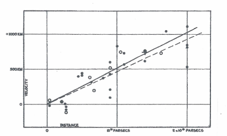
Figure 1: [Hubble’s original caption]
Velocity-Distance Relation among Extra-Galactic Nebulae.
Radial velocities, corrected for solar motion, are plotted against distances estimated from involved stars and mean luminosities of nebulae in a cluster. The black discs and full line represent the solution for solar motion using the nebulae individually; the circles and broken line represent the solution combining the nebulae into groups; the cross represents the mean velocity corresponding to the mean distance of 22 nebulae whose distances could not be estimated individually. ©US National Academy of Sciences.

The coefficient $H$ in (12) (which Hubble himself denoted $K$) is known as the Hubble constant, although it varies with time in observationally viable FLRW models: Hubble estimated it as 500 km/s/Mpc. (He actually found $H=465\pm 50$ km/s/Mpc from the 24 galaxies and $513\pm 60$ km/s/Mpc by treating them in 9 groups.) Lemaître’s analysis had been done with and without a weighting intended to reduce the influence of the more distant galaxies on the result, as the observations of those galaxies seemed less reliable, and he found $H=575$ (without the weighting) and $H=625$ (with it), in km/s/Mpc. It is worth noting that, like Eddington and Lundmark, Hubble refers only to redshifts in de Sitter space and not to the Friedman-Lemaître expanding models. Other leading scientists remained unaware of the expanding universe interpretation, or, preferring a static picture, were initially unconvinced by it. Hubble himself is quoted by his biographer as saying in 1937 “Well, perhaps the nebulae are all receding in this peculiar manner. But the notion is rather startling” [Chr95, p. 201] and even in his Darwin Lecture [Hub53] talked of competing interpretations and said the law should be regarded as “an empirical relation between observed data”. The reasons why others failed to pick up on Lemaître’s discovery are considered by Luminet in his excellent editorial note to the recent reprint [Lem13]; only in 1930, when Lemaître sent a copy of his paper to Eddington, who then forwarded it to de Sitter and Shapley, did the expanding model come to the fore. Edd30 also discovered the instability of the Einstein static metric to small changes of the parameters (whence his name is attached to the Eddington-Lemaître model). This proof and his advocacy of Lemaître’s work led to the wide acceptance of the evolving models, although in Edd30 he noted that “it is possible that the recession of the spirals is not the expansion theoretically predicted; it might be some local peculiarity…”, a good point in view of the small sample then available. Ein31 then renounced the cosmological constant and considered a Big Bang model with recollapse [ORaMcC14]. In the English version of Lemaître’s 1927 paper, published in 1931, the part on the magnitude-redshift relation is omitted. Research by Liv11 found that this was not, as has sometimes been claimed, a change made editorially, but was made by Lemaître himself. Why that was done remains unclear. Luminet has discussed the other changes made in the 1931 version.

3 Measuring the Hubble “constant”

3.1 Measuring and interpreting redshifts

Redshifts of galaxies can be rather accurately measured. This is done by identifying patterns of lines in spectra which are characteristic of emission or absorption by particular atoms or molecules, and comparing the observed frequencies with those measured in the lab. The method does of course assume that the emitted frequencies are not affected by the evolution of the Universe, and some explanations have abandoned that assumption. It has been examined in a number of works over the years, the most recent being centred on discussions of possible variations in the constants of nature, principally the dimensionless fine structure constant $\alpha$. Variation in both time [MurWebFla03] and space [KinWebMur12] has been claimed, the latter showing a dipole which may be correlated with that of other indicators [MarPer13]. Such a variation can be described as a variation of any of the dimensionful constants used to define $\alpha$, e.g. the velocity of light $c$. The claimed, and still controversial, observed variation is small enough that it does not significantly affect measurement of the Hubble constant. Treating light in the geometric optics approximation, one can show that if $k^{a}$ is the vector tangent to a light ray from an emitter G to an observer A, and objects have four velocities $u^{a}$, then the red- (or blue-) shift observed by A is given by

$$1+z=(u^{a}k_{a})_{A}/(u^{a}k_{a})_{G}.$$ (13)

If the $u^{a}$ are the velocities of timelike lines in the flat (Minkowski) space of special relativity, then for purely radial relative motion the redshift would imply a recession velocity $v$ given by

$$1+z=\sqrt{\frac{1+v/c}{1-v/c}},$$ (14)

the Doppler effect. For $v$ small compared with $c$, $z\approx v/c$. Since flat space is a good enough approximation to general relativistic geometry out to a distance given by a square root of the magnitude of the Riemannian curvature components, using the velocities given by (14) was a good enough approximation for Hubble and remains a good one for considerably larger distances. (From (15) below, to a redshift $z>1$ with current $\Omega_{m}$ and $\Omega_{\Lambda}$ values in (2.2).) However, within general relativity the expanding universe models are not flat. Since $k^{a}$ is geodesic, the change in the $(u^{a}k_{a})$ of (13) along a ray is due to the difference between $(u^{a})_{G}$ parallel-transported from G along the ray to A and $(u^{a})_{A}$. This has to be computed using the equations for geodesics in the curved space and the assumed motions of the emitter and observer, which are usually taken to be those of comoving or “fundamental” observers in an FLRW model, i.e. those at constant spatial coordinates. For such observers this gives exactly the ratio of the spatial distances between them at the times of emission and reception, cf. (10); there has thus recently been some debate about whether the redshift should be thought of as due to a Doppler effect or not [Kai14]. One aspect of the argument has been that the calculation does not involve the Riemann tensor, only the connection, and therefore should not be considered gravitational: however, the Riemann tensor and its derivatives completely determine local geometry, including the connection (see e.g. Theorem 9.1 in SteKraMac03). One should note that galaxies and other sources with measured redshifts will not be exactly following worldlines of fundamental observers in a best-fit FLRW model. They will have “peculiar motions” relative to that velocity. These tend to be small compared with the cosmic expansion velocities, e.g. they are not more than a few thousand km/s against the velocity of $\approx 2\times 10^{5}$ km/s at redshift 1 implied by (14). While thus not critical in deriving the Hubble constant, measured peculiar motions are of great importance in identifying large scale gravitating structures such as the Great Attractor [LynFabBur88]. At the present time observed redshifts range up to 8.6 [LehNesCub10], and candidates in the range of $z$ 8.5-12 have been identified [EllMcLDun13]. Spectral lines in visible light are not the only way to measure redshift. One can also measure it from, for example, the 21cm line of neutral hydrogen, common in both absorption and emission by intergalactic gas clouds. The origin of redshift in an expanding pseudo-Riemannian geometry is clear, but there have been a number of controversies about this FLRW interpretation. Apparent physical associations between objects of different redshifts led to a prolonged debate [FieArpBah73]. Other authors thought there was a “tired light” contribution, or banding of redshifts within clusters.

3.2 Establishing the distance scale

Redshifts are relatively easily and well measured. Measuring the true distances is much trickier: it is this which makes giving an accurate absolute value for $H$ hard. The full story of how astronomical distances are obtained involves a great many astrophysical phenomena and techniques, and has generated a series of subjects of debate over several decades. By itself, it merited a very good book [Row85]; and there have been subsequent developments, probably including some of which I am unaware. So what follows is just a short summary. The principal idea, in measuring distance to other galaxies, is to measure the flux received from a “standard candle” for which an actual, intrinsic, luminosity $L$ (the total output, or the output at given frequencies) is known, and then infer the distance by comparing the observed flux and the intrinsic luminosity. Standard candles are usually assumed to radiate isotropically. There are several obvious problems with this procedure: sources do not emit uniformly across different frequencies, so one wants to make the measurements in such a way that the intrinsic luminosity and observed flux refer to the same rest frequency; standard candles are not strictly standard and one has to allow for the intrinsic variations between members of a class, and possible resulting selection effects; and to increase the distance range covered one has to use intrinsically brighter standard candles, meaning one has to calibrate the intrinsic luminosity of the new class from members of it which are clearly at the same distance (e.g. because they are in the same galaxy) as members of known fainter classes. The series of increasingly bright classes form the “distance ladder”. For those new to this topic, the situation is complicated by astronomers’ adherence to magnitude and parsec, rather than SI, units. Magnitudes $m$ arose in ancient astronomy. The Greeks classed the brightest stars as being of first magnitude, the next brightest as second magnitude, and so on: higher magnitude objects are thus fainter. Because the eye responds essentially logarithmically to received light, this means that the magnitude $m\propto-2.5\log_{10}L$ for sources of intrinsic luminosities $L$ at a fixed distance: the factor 2.5 was proposed by Pogson in 1856 so that 5 magnitudes corresponds to a factor 100 in luminosity, agreeing to a good approximation with historic values for $m$. To complicate matters, the zero of magnitude depends on wavelength, and on the stars or other objects taken as calibration standards (see e.g. Bes05). The two main systems now in use are the Vega (or Johnson) system and the AB system. The AB system is defined so that zero magnitude is 3631 Jansky in every band, where 1 Jansky $=10^{-26}W/m^{2}/Hz$. The Vega system, originally defined so the star Vega had zero magnitude in all bands, has been revised so that Vega is now magnitude 0.02-0.03. The two systems are close in the visual V band but, for example, in the near infra-red K band differ by 1.85 magnitudes. (As a historical note, a table produced by Hale Bradt in 1979 gave, for the wavebands U, B and V much used in the past for photometric data, the values 1896, 4267 and 3836 Jansky in those bands.) Apparent magnitude $m$ is given by the measured flux, in $Wm^{-2}$, in the relevant waveband. Absolute magnitude $M$ is defined as the apparent magnitude the source would have if at a distance of 10 pc. For extended objects this has to be interpreted as the magnitude a point source of equal luminosity would have at that distance. Then, assuming an inverse square law for brightness, the “luminosity distance” $D_{L}$ is given in pc by

$$M-m=-2.5\log_{10}(D_{L}/10)^{2}\Rightarrow D_{L}/(10~{}{\rm pc})=10^{0.2(m-M)}.$$

The definition of luminosity distance implicitly assumes that there is no redshift between G and A. Redshift factors affect distance measurements in two ways: they affect cross-sectional area measurements of beams of light by relatively moving observers, and produce spreading out of the spectrum. If one defines the observer area distance in terms of the cross-sectional area ${\mbox{\rm d}}S_{G}$ of the observed object G and the solid angle ${\mbox{\rm d}}\Omega_{A}$ it subtends at A by

$$r_{A}^{2}:={\mbox{\rm d}}S_{G}/{\mbox{\rm d}}\Omega_{A},$$

then $D_{L}=(1+z)^{2}r_{A}$. Similarly one can define a distance $r_{G}$ from the solid angle ${\mbox{\rm d}}\Omega_{G}$ subtended at G by an area ${\mbox{\rm d}}S_{A}$ at A using $r_{G}^{2}:={\mbox{\rm d}}S_{A}/{\mbox{\rm d}}\Omega_{G}$; then $D_{L}=(1+z)r_{G}$, $r_{G}=(1+z)r_{A}$. When dealing with fluxes in specific intensity ranges (per Hz), one also has to allow a $(1+z)$ factor relating the widths of the wavebands. Past authors have not always been clear about what distance measure they meant, and thus the various factors of $(1+z)$ were not always treated correctly. It should be noted that as a consequence of the relations between the distance measures, a check on the value of $D_{L}$ is in principle supplied by measuring $r_{A}$, assuming one knows $z$ and the intrinsic cross-sectional area of a class of objects. The resulting analogue of the $m-z$ relation is usually denoted the $\theta-z$ relation, where $\theta$ is the measured angular diameter of the objects. The first step in establishing the distance ladder is measurement of trigonometric parallax, the same technique humans and other animals with two eyes set apart use to infer distance. In astronomy one observes the (small) change in the direction in the sky of an object, usually a star, when the Earth is at opposite points of its orbit round the Sun (i.e. 6 months apart). The parallax is then one half of this, so it is $R_{\oplus}/D$ where $R_{\oplus}$ is the radius of the Earth’s orbit and $D$ is the distance. (For this purpose one can assume Euclidean geometry.) One parsec (pc) is defined as the distance at which an object in a direction perpendicular to the Earth’s orbit has a parallax of one arc-second. The known size of the Earth’s orbit ($R_{\oplus}$ is roughly $1.5\times 10^{8}$ km) gives the SI units value of this (to 1 d.p.) as $3.1\times 10^{13}$ km: one parsec is 3.26 light-years. Distances within the Galaxy lie in a range from about 1.3 pc (the distance to Proxima Centauri, the nearest other star to the Sun) to 20 kpc or so. M31 is at a distance of about 800 kpc. Distances to the most distant galaxies measured by standard candle type methods are of the order of Gpc. In modern galaxy surveys, Hubble’s law is inverted in order to infer (relative) distances from redshifts and so derive separations and maps of structures. Classical observations using parallax could lead to errors as much as 10% at 30pc. A major target was and is the Hyades open cluster, a group of stars used to calibrate methods used to make the next steps, such as using stellar spectroscopy to identify stars which have common properties and so can be standard candles, and the technique of main sequence matching, described briefly below. The Hyades is the open cluster nearest to us and is in the constellation Taurus: its stars have been and are studied in great detail. More recently, parallaxes have been measured using satellites such as Hipparcos and the Hubble Space Telescope [deHoode01, McABenHar11]: the GAIA satellite which commenced observations in 2014 is expected to enhance these considerably. At the distances accessible to direct parallax measurement, other methods which are used as confirmations or checks include cluster parallaxes (using apparent convergence of proper motions, i.e. tangential velocities as seen from Earth) and statistical parallaxes of some sample of stars. From these observations, the Hyades are now agreed to lie at about 47pc. Calibrating by Hyades stars, one can use stellar spectroscopy for individual stars, and the position in the luminosity-temperature diagram (the Hertzsprung-Russell diagram) of the zero-age main sequence, the curve which newly formed stars settle to as they enter the phase in which their energy mainly comes from fusing hydrogen to helium. A next step in the ladder comes from the period-luminosity or period-luminosity-colour relations for variable stars (the first of these, for Cepheids, had been discovered by Henrietta Leavitt in 1908). RR Lyrae stars, W Virginis stars and Cepheids have been used, with various difficulties of calibration. These indicators, together with novae and supernovae, can be regarded as primary indicators, enabling calibration of secondary indicators which can be used in parallel to observe to even greater distances [Row85]. The supernovae considered as primary indicators are of two types (these do not cover all supernovae). For both types, decay of unstable radioactive isotopes, notably ⁵⁶Ni, formed by the explosion is an important, and for SN1a the only, source of the light. Type II supernovae, those with no hydrogen lines in the spectrum, are due to core collapse of young massive stars, and are seen in spiral galaxies. Theoretical models of surface brightness (in the simplest case, assuming a black-body spectrum) and the observed luminosity can be used to derive an angular size and this can then be combined with Doppler redshift measurements to obtain the velocity of expansion and thus the linear size and distance: this is called the Baade-Wesselink method. Type I supernovae have great homogeneity in the time variation of their luminosity and colour. They are believed to be due to a white dwarf exploding because accretion had raised its mass above the Chandrasekhar mass limit: evidence for this has come from observations of NugSulCen11, but there is still uncertainty about the origin of the accreted mass. Type Ia (the ones with a strong ionised silicon absorption line) are the brightest: see section 5 for the resulting $m-z$ data. Over 100 were known by the 1980s and new ones are now being discovered at a rate greater than 2000 per annum. Secondary indicators include ionised hydrogen (HII) regions, the brightest globular clusters in a galaxy, the brightest stars in a galaxy, the Tully-Fisher relation between the luminosity of spiral galaxies and the width of the 21 cm emission of neutral hydrogen atoms in those galaxies, and finally overall properties of galaxies (colour-luminosity relations, luminosity classes, sizes, brightest cluster galaxies). Hubble based his distance measurements on observations of Cepheid variable stars, calibrated by observations in the Galaxy. Unfortunately, as I now discuss, the variable stars he was observing in M31 and other galaxies were not Cepheids, but the similar but less bright type of variable, the W Virginis stars. He then used these measurements to calibrate the “brightest star” indicator, and so could find galactic distances with both methods, but of course with incorrect overall scale.

3.3 Measured magnitude-redshift relations

The first major revision of Hubble’s results was brought about by the commissioning of the Mount Palomar 200 inch telescope in 1950. Baade used it to observe M31. Had Hubble’s distance been correct, Baade should have been able to see RR Lyrae stars, and he could not. The identification of two stellar populations arose in this work. The two populations are distinguished by their metallicities. Baade realised that the two rather similar types of variable, W Virginis stars and Cepheids, in the two populations had been conflated by Hubble. W Virginis stars (or type II Cepheids) are Population II stars with brightest magnitudes around $-3.5$ whereas (type I) Cepheids are Population I stars with brightest magnitudes about $-5$. Disentangling the two led to revision of Hubble’s distance scale by a factor of about 2.5. Because the principal uncertainty in magnitude redshift relations lies in the distances, cosmologists often use a parameter $h=H/100$, where $H$ is in km/s/Mpc. The Hubble age, $1/H$, is then approximately $10/h$ Gyr. Baade’s $h$ was about 2. The next big revision arose from Sandage’s 1958 discovery that HII (ionized hydrogen) regions had been misidentified as stars: he noticed that they looked too red to be stars, as a result of the Balmer lines registering on red plates. Sandage gave a value $h=0.75$; by 1975 he was using galaxies out to redshifts above 0.3, i.e. ten times Hubble’s most distant objects. Baade and Sandage’s discoveries not only ushered in a new phase in cosmological science, as described in Section 4.2, they also provided the final step in establishing the “Copernican Principle” that humanity has no special position in the Universe. Copernicus and Galileo had argued that the Earth was not the centre of the Solar System, and Shapley, Lindblad and Oort had proved the Sun was not at the centre of the Galaxy. The revised distance scales now showed the Galaxy was not the uniquely largest in the Universe. (The recent discovery of many planets orbiting stars other than the Sun, some possibly habitable, provides further evidence against humanity having a special position in the physical Universe: as yet the existence of intelligent life on extrasolar planets remains conjecture rather than confirmed fact.) There was considerable debate about the correct value for $H$ after 1958, in which values between about 54 and 100 were obtained by various sets of new observations and analyses. (Geoff Burbidge used to show a log-log graph of the estimated age of the universe against the date on which the estimate was made, which was linear starting from Bishop Usher’s estimate of 6000 years. He thus claimed that if it was known when the next revision would occur one could predict its value.) Nevertheless, the current best estimates essentially agree with Sandage’s 1958 figure. It has been suggested that there are variations of $H$ with direction, in particular a dipole variation due to the motion of the Galaxy with respect to other galaxies. One difficulty in studying this lies in relative distance scale calibrations for different directions. The value of $H$ appears in a linear approximation for the $m-z$ relation at small $z$. Such a relation applies for any congruence of worldlines of galaxies and observers with four-velocities $u^{a}$ in a relativistic spacetime, and in this case $H={u^{a}}_{;a}/3$. To study the relation at greater $z$ one needs a more accurate model. Observationally, it is natural to approximate the relation as a series: the coefficient of the first nonlinear correction then gives the value of $q$. The relevant expansion for sources of equal intrinsic luminosity in an FLRW model reads

$$m=5\log z+1.086(1-q)z+O(z^{2})+\mbox{\rm constant}.$$ (15)

One can extend this series, and calculate series for other measurements, not only for FLRW models but also for models with anisotropy and inhomogeneity [KriSac66, MacEll70], but such approximations become poor ones at the large redshifts now observed. It is more usual now to compare data with numerically computed relations. The numerous attempts up to the 1990s to obtain observations sufficiently accurate to obtain $q$ from (15) (as suggested by Hub38) ran into various experimental and theoretical problems. These included the K-correction (relating fluxes from different emitted frequencies), aperture correction (to make sure the flux is solely and wholly from the intended object), absorption in the Galaxy and the intergalactic medium, the effects of lumpiness arising because the matter density within the observed beams of light differs from the average density [DyeRoe74], selection effects (which arise, e.g., from favouring the brightest in a standard candle class) and the unknown evolution of the sources. Estimates varied from about 0.25 to 1.6. The most prominent recent method for measuring the magnitude redshift relation has used supernovae of type Ia. As described in section 5 below, this led to the first good measurement of $q$, i.e. of the time variation of $H$, giving a value which has since been shown to be consistent with data from baryon acoustic oscillations and gamma ray burst sources. Yet more ways of obtaining and extending $m-z$ may become available soon. For example, the use of reverbation mapping of AGNs and quasars, which exploits the time delay between variations in the continuum and line emission regions round AGNs and quasars and the theory of accretion disks, could obtain sizes and hence distances, and gamma-ray burst sources appear to extend the SN1a relation to much higher redshifts. It is perhaps disappointing that the correct value of $H$ is still rather uncertain. Calibration of the SN1a data, still using Hubble’s classic method of observing Cepheid variables, leads to a value $73.8\pm 2.4$ [RieMacCas11], while the Planck data [AdeAghArm14] gives $67.3\pm 1.2$. This illustrates how hard it is to obtain precise cosmological distances even now, 85 years after Hubble’s work.

4 Modeling the expanding universe, after 1929

4.1 Modeling Hubble’s results

There were many papers after 1929 exploring expanding universes, though initially most avoided the singular ones, i.e. the Big Bang cases. It was again Lemaître who took the lead in realizing the significance of the singular models [Lem31]. However, once the concept of expansion had become generally accepted it was clear that FLRW models agreeing with Hubble’s data almost all expanded from a Big Bang. Only the Eddington-Lemaître models asymptotic to the Einstein static model as $t\rightarrow-\infty$ avoided a singularity, and they were unstable. There are models that “coast” close to the Einstein static model for a period: these were invoked at one time to explain an apparent clustering of quasar redshifts around 1.95 but no such effect is now believed to exist. Thus by the time of Rob33’s review Rob33, the behaviour of all the FLRW models was pretty well understood. In summary, the generic behaviours possible are illustrated by Fig. 2, assuming $\mu$ and $p$ are positive in the case $\Lambda=0$.

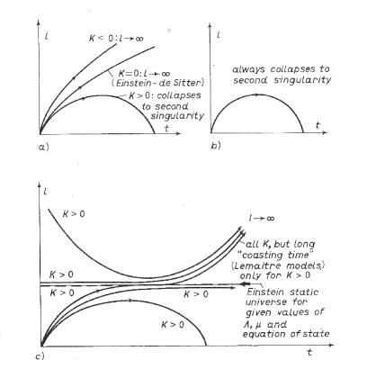
Figure 2: Scale factor $a(t)$ for (a) $\Lambda=0$, (b) $\Lambda<0$, (c) $\Lambda>0$. From Figure 9.1 of EllMaaMac12, itself adapted from Fig. 4 of Ell71.

At small $a$ the $\Lambda$ and $K$ terms in (6) are negligible. Then for $w=0$ (“dust”) we have $a\propto t^{2/3}$, and for $w=1/3$ (“radiation”), $a\propto\sqrt{t}$; the corresponding exact solutions are due to Einde32 and Tol34. For constant $w$ (other than -1) one obtains $a\propto t^{2/3(1+w)}$. At large $a$, $\Lambda$, if non-zero, will give the dominant term: if $\Lambda=0$, then, assuming that pressure asymptotically vanishes as $a\rightarrow\infty$, the value of $K$ determines the far future behaviour (re-contraction if $K=1$, expansion for ever if $K=-1$, approaching the Milne solution $a\propto t$ which is flat Minkowski space in FLRW coordinates, and convergence to the Einstein-de Sitter model if $K=0$). As noted above, $\Omega_{r}$ is negligible for most of the life of the Universe (for $t>t_{eq}$), although it is the dominant term between the end of inflation and $t_{eq}$. On the other hand, $\Omega_{\Lambda}/\Omega_{d}\propto a^{3}$ implies that a nonzero $\Lambda$, or more generally dark energy in any of its proposed forms, becomes dominant at late times in an FLRW expansion. Since $\Omega_{K}/\Omega_{d}\propto a$, $K$ is dynamically unimportant at small $a$, and for realistic FLRW models only becomes dynamically important at large $a$ if the dark energy contribution decreases faster than $\Omega_{K}$. Nonzero $K$ is the generic case, but the recent evidence for nonzero $\Lambda$ has meant that the effort expended on determining $K$ has lost part of its motivation, since a value $K\neq 0$ may not be critical in determining the future behaviour of the expansion. That $\Omega_{K}/(\Omega_{m}+\Omega_{\Lambda})$ is small is consistent with inflation, as discussed above. Taken together, these remarks, together with the considerations on thermal history (see below and Dur15), show why it is usual to adopt a Tolman model in the early universe and a dust model at late times (moderated, nowadays, by the inclusion of $\Lambda$ in recent epochs). The main reason why expanding models were not universally accepted immediately after 1929 was that if (12) were universal and $H=500$ had remained constant as the Universe evolved, interpretation as an expanding universe implied a “Hubble age” $1/H$ for the Universe of 2 Gyr. With $\Lambda=0$ and positive $\mu$ and $p$ the Hubble age is an upper bound for the age of an FLRW model. Hubble’s value for $1/H$ was less than the age of the Earth, which was known to be about 4.5 Gyr. That discrepancy led to the consideration of various alternative theories of gravity and cosmology, although most of the alternatives also considered the universe to be expanding: for fuller accounts of them see Nor65 and Bon60. Among the alternatives the most widely considered (at least in the UK) was the Steady State theory first developed by BonGol48 and Hoy48. This used (9) as the metric, so the universe expands in this theory: it manages to remain the same at all times due to continuous creation of new matter. Steady State theory had nice simplifying features and produced definite predictions, whereas Big Bang theory had some unknown parameters: accordingly Steady State attracted a strong body of proponents. Age problems involve not only the Earth’s age. Until the 1920s, the only known source of the required energy for a star was the gravitational potential energy of the star, but this “contraction hypothesis” led to a maximum age around $2\times 10^{7}$ years, in conflict with “biological, geological, physical and astronomical arguments” (to quote Eddington). From about 1920 onwards (see Edd26) it was recognized that the power source was nuclear fusion, for main sequence stars the fusion of hydrogen to helium (another insight arising from relativity, in this case Einstein’s deduction within special relativity of the famous $E=mc^{2}$). Estimates of stellar ages are subject to significant uncertainties, due to the complexities of modelling stellar evolution. The greatest currently estimated age of an observed star is $14.5\pm 0.8$ Gyr [BonNelVan13] which is very close to current estimates of the time back to the Big Bang. Baade’s distances led to a Hubble age of 5 Gyr, just about compatible with the age of the Earth. The age of the Galaxy was then estimated to be between 3 and 15 Gyr, on the basis of data from meteorites, stellar evolution and dynamics, and observations of interstellar dust [Bon60], so this too could just about be accommodated. These age estimates became comfortable after Sandage’s revision, which led to a Hubble age of about 13 Gyr and removed that motivation for alternative theories. Despite the age problem, FLRW models continued to be investigated between 1929 and 1952, if perhaps more slowly than they might have been, and some aspects which have since assumed ever-increasing significance were first explored. The idea of remnant radiation from the Big Bang arose in Lem31, but the resultant black-body spectrum and decoupling were not discussed then and Lemaître thought cosmic rays might be the remnant. Our current picture is of course that baryonic matter and radiation are strongly coupled in the early universe, that the relevant temperatures therefore evolve together, and that the coupling ends at a temperature around 3000K (more accurately, at about $z=1089$) although the radiation remains thermal (black-body). After decoupling, the radiation propagates freely (or, possibly, interacts with a reheated intergalactic medium). The decoupling happens rather abruptly and thus can be characterized as happening at a specific surface $t=t_{dec}$, the “last scattering” surface. Tolman considered the thermodynamics of Big Bang models, including the effect of expansion on black-body radiation temperature and of a gas in equilibrium with it [Tol34]. However, he did not infer the presence of the CMB. That was predicted later, when the lack of equilibrium, which is forced by expansion [SteMacSci70], was brought into play to discuss element formation, in work which also led to the theory of primordial nucleosynthesis. Such nucleosynthesis was first considered by Gam48, in a series of papers from 1942 onwards. He recognized the need for high temperatures to enable neutron capture, and the possibility of this for a limited period in the expansion of radiation-dominated models [Gam46, Gam48]. Alpher, Herman and colleagues developed this further, and carried out detailed nucleosynthesis calculations. They also predicted the CMB at a temperature of 5K [AlpHer49]. The outcome of these calculations was that primordial nucleosynthesis could produce the light elements but not the heavy ones [AlpFolHer53, Gam56]. The mechanism to form light elements starts with neutron-proton merger to form deuterium followed rapidly by a series of reactions to form $He^{4}$. The deuterium is instantly dissociated by incident photons if $T\geq 8\times 10^{8}$K. Neutrons decay to protons with a half-life about 660s and after this has happened no more deuterium forms. So the outcome depends on the neutron-proton ratio when $T=10^{8}$K, which gives the initial condition for deuterium formation, and the time scale of expansion, which causes collision rates to drop as density does. It was Hay50 who pointed out that the initial ratio arose from processes with high $T$ dependence which would give a thermal equilibrium until their time scales became slow compared with expansion. Taking that into account the helium to hydrogen ratios came into good agreement with observation. WagFowHoy67 refined the calculations and included elements up to Li⁷. The theory of production of heavy elements in stars was developed by BurBurFow57 in the context of the Steady State theory. This work showed such synthesis could not produce the observed deuterium. Stellar nucleosynthesis complements the primordial element production in giving the observed species. Another important topic opened up in this period was the theory of perturbations of expanding models. Newtonian models were considered by various authors, notably Bon56: Lif46 was the first to obtain a growth law for perturbations in relativistic models and introduced methods followed in later work. However, until 1980 there were no plausible ways to generate the necessary perturbations. For example, in giving a summary of what was then known, Har73 noted that if thermal fluctuations provided the seeds for galaxies, they had to be generated between $10^{-31}$ and $10^{-29}$ s after the Big Bang. Yet another topic introduced in this era was the study of inhomogeneous and anisotropic models (see chapters 17-19 of EllMaaMac12 for a recent review of these). Lem33 introduced the spherically symmetric dust models now called the Lemaître-Tolman-Bondi (LTB) models, in order to model collapse of overdense regions into galaxies. In the same paper he considered, after a suggestion from Einstein, the spatially homogeneous anisotropic Bianchi I models, in order to illustrate that the singularity at the Big Bang of the FLRW models was not unique to that case.

4.2 Modeling with improved distance scales

In the 1960s two observational developments in particular, the counts of radio sources and the detection of the CMB, gave the Big Bang view the edge over Steady State (although Steady State enthusiasts continued for some time to try to incorporate these observations within their theory). The cosmic radio source count data showed that the universe was not only expanding but evolving. It did so by plotting source count numbers $N$ against radio flux $S$, so proving that the number of radio sources in the past was higher than today by more than could be accounted for by geometric effects in any reasonable model. The data from which this inference was initially drawn was inadequate, due to confusion between sources etc. but by 1968 these systematic errors had been corrected [PooRyl68]; see Figure 3.

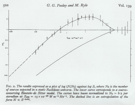
Figure 3: The $N-S$ curve from PooRyl68, Fig. 2, and its caption

Therefore the population of radio sources, and thus the Universe itself, had to be evolving. Unfortunately, the intrinsic variations between radio sources and the lack of detailed understanding of their evolution makes it hard to gain other cosmological information from them. The earliest paper to re-examine the CMB prediction was by DorNov64 but, as described by Nov09, its significance remained unappreciated, as did data by Shmaonov and the observations of the CN molecular lines. For discussion of the discovery by Penzias and Wilson and subsequent observational and theoretical work see Dur15. The presence of the CMB confirmed the evidence from element abundances, showing that the universe had been through a hot dense phase, and had thus come from a Big Bang. The generally accepted thermal history for FLRW models now started with a Tolman radiation universe with known ratio $a/\sqrt{t}$ (see Dur15), followed by a “matter era” driven by dust but with unknown $\Omega_{d}$. Isotropy about our position in space was shown at that time by a number of tests. Galaxy number counts were only known to be isotropic to about 30% (the uncertainty being due to the clustering), but the radio source counts and X-ray background were isotropic to better than 5% and the CMB was known from about 1969 onwards to be isotropic to better than 0.2%. The first anisotropy measured in the CMB, in 1969, was the dipole due to the motion of the Sun relative to the frame in which the CMB is most nearly isotropic (see Dur15 for details and references). In contrast, then and now, obtaining clear evidence for spatial homogeneity is difficult in that we do not receive data from objects separated from us in space but not in time. In particular we cannot in principle separate space and time evolution, since, apart from “geological evidence” in our local neighbourhood, our observations are on our past null cone. So to infer homogeneity implies assumptions about how the matter content behaves away from the null cone. It is not even easy to test the assumption that there are spacelike surfaces of approximate homogeneity extending to large distances. For example the surface of last scattering might be a timelike cylinder intersecting our past null cone in the sphere we actually observe [EllMaaNel78] (though the particular model where this was considered is ruled out by other considerations). Even when one takes the more usual assumption that last scattering occurs on a spacelike surface, one needs to be able to apply some theory of the evolution objects undergo between the emission of the received radiation and now. These assumptions are hard to test. Thus to improve tests of homogeneity we would need to have a much better understanding of evolution of galaxies, radio sources and other objects than we do. We are however able to make two types of tests: we can check that there is no local evidence for inhomogeneity, for as far back in time as we feel confident about our understanding of evolution, and we can test for the presence of significant mass variations which are asymmetrically arranged about us by looking for their effects on the CMB. The tightest bounds of the latter type seem to be those of ZibMos14. Thus in the 1960s and 1970s it was becoming ever clearer that the FLRW models satisfied the observational requirements of expansion, evolution, a hot dense phase, and apparent isotropy and spatial homogeneity. They accounted for the evolution of the light elements, while nucleosynthesis in stars accounted for the heavy ones, and they naturally gave rise to the CMB. The value of $H$ was believed to be at most 100, and therefore there was no serious age problem. The models still had significant unknown or poorly known parameters: $\Omega_{d}$, $K$, $q$ and $\Lambda$. They also did not predict the baryon number $B$, the ratio of the number of photons per unit volume (in the CMB) to the corresponding count of baryons, which is a measure of entropy and affects the helium/hydrogen ratio and other light element fractions, and so on. There were attempts to obtain the FLRW model parameters not only from the $m-z$ relation but also the $\theta-z$ and $N-S$ relations described above, the $N-m$ relation for galaxies (a test proposed by Hub36), and the $<V/V_{max}>$ test, where $V$ is the volume of a sphere of radius given by the distance of a source and $V_{max}$ the maximum volume within which it would be detectable: precise values remained elusive. It became clear that there was dark matter in the universe (see LonRee73 or ColEll97). The phrase “missing matter” came into use, but rather confusingly was used both for the mass inferred to be in galaxies and clusters in addition to their visible mass (which pointed to an $\Omega_{m}$ of about 0.3: see the references immediately above) and by those who believed that the true $\Omega_{m}$ was 1, although there was no observational evidence for such a large value (or for a non-zero $\Lambda$). The period saw some important steps in understanding light propagation in the Universe. SacWol67 worked out the effects on the CMB of gravitational redshifts: the fully non-linear integrated effects were discussed by ReeSci68. SunZel70 described the effect of inverse Compton scattering in galaxies on CMB observation. See Dur15. Several papers, notably those of DyeRoe74, considered light propagation in lumpy models. One aspect of FLRW models studied in greater detail was the impact of the exact rate of expansion during element formation (which depends on the particles present and on the anisotropy) on the resultant ratio of atomic species. SteSchGun77 showed that such cosmological considerations limited the number of neutrino species, at that time unknown but expected from the quantum theory of the standard model of particle physics to be 3, to at most 5. A more recent re-analysis [CybFieOli05] gave $2.67\leq N_{\nu}\leq 3.85$ at the 68% confidence level, while Planck’s data gave $N_{eff}=3.30\pm 0.27$ [AdeAghArm14]. Similarly, Bar76 used the effect of anisotropy on the expansion rate to give a limit $10^{-7}$ on present-day anisotropic shear $\sigma$, possible because a $\sigma^{2}$ term has to be added to the Friedman equation (6). Big Bang FLRW models have a singular origin. The understanding of singularities, defined as the presence of geodesics which could not be indefinitely continued, developed considerably during the 1960s and 70s. Theorems proving their existence in relativity (see HawEll73, TipClaEll80 and the Milestone “The singularity theorems (1965)”) were complemented by examples of possible behaviours and by the work reviewed in BelKhaLif82 aimed at describing singularities’ generic form. As a result of the CMB discovery, it was possible to prove that a relativistic cosmology that was expanding approximately like an FLRW model had to have had a trapped surface in the past and therefore must have had a singularity in the past [EllHaw68].

5 Modern relativistic cosmology

5.1 Observations

Three important sources of observational data, the anisotropies in the CMB, the $m-z$ relation itself, and galaxy surveys, have undergone major developments since the 1980s. Combining the results has given a much stronger base for our modeling. Moreover, other sources of data have been and are being added. The first to improve was the measurement of the fluctuations in the CMB (beyond the level of the dipole due to the Earth’s motion), discussed more fully by Dur15. This has evolved from the first indications in the COBE data of the early 1990s through to the very detailed recent results by Planck (e.g. AdeAghArm14) and a number of ground-based telescopes. There are ongoing observations by the ever-increasing number of ground-based instruments which will give us further fine detail. Drawing the implications from this data depends on calculating the evolution of fluctuations from the input fluctuation spectrum predicted to have been formed during inflation, within an FLRW model (see section 5.2 and Dur15). Comparing such calculations with the observations puts constraints on the expansion parameters $H$, $\Omega_{m}$, $\Omega_{K}$ and $\Omega_{\Lambda}$. Note that these parameters give rise to accumulated effects over a long period, rather than referring to measurements of relatively nearby objects. The most unexpected addition to previous data came from the Hubble relation for supernovae of type 1a. It was unexpected because if $\Lambda=0$, as was generally believed, then (11) shows that the expansion rate should be decelerating. The result, first announced in 1998, showed instead that $q<0$, implying $\Lambda>0$: it won the lead scientists the 2011 Nobel prize. The CMB observations show a first main peak in the power spectrum, from which a length scale at the time of the last scattering of the CMB can be inferred. Expansion will then fix the corresponding length scale for a peak in the distribution of galaxy-galaxy separations at a later time. This is the BAO measurement, made in surveys of galaxies. Taking galaxies in a given band of redshift, around a value $z_{B}$ say, allows one to estimate the evolution between the time of last scattering and $z_{B}$ and thus the $\Omega$ values, assuming an FLRW model. The BAO peak is a less than 1% deviation from a uniform distribution. Nevertheless it can be measured with considerable, albeit model-dependent [RouBucOst15], accuracy. The same peak has recently been measured using the Ly$\alpha$ forest in the spectra of quasars at redshifts in the range $2.1\leq z\leq 3.5$ [DelBauBus15]. Using this data and a value for the sound horizon obtained from the Planck data leads to a value for $H$ at $z=2.34$ of $222\pm 7$, about 7% ($2.5\sigma$) discrepant with a flat $\Lambda$CDM cosmological model with the best-fit Planck parameters. The accumulated SN1a data has been compared with the BAO measured by the WiggleZ team [BlaKazBeu11] at several redshifts out to $z>0.7$ and agrees very well; see Figure 4.

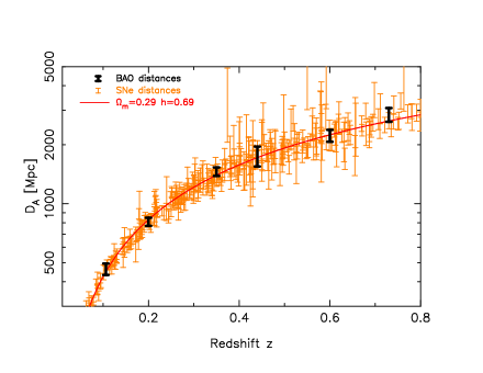
Figure 4: [Caption from BlaKazBeu11] Comparison of the accuracy with which supernovae and baryon acoustic oscillations map out the cosmic distance scale at $z<0.8$. For the purposes of this Figure, BAO measurements of $D_{V}(z)$ have been converted into $D_{A}(z)$ assuming a Hubble parameter $H(z)$ for a flat $\Lambda$CDM model with $\Omega_{\rm m}=0.29$ and $h=0.69$, indicated by the solid line in the Figure, and SNe measurements of $D_{L}(z)$ have been plotted assuming $D_{A}(z)=D_{L}(z)/(1+z)^{2}$.

Values for $\Omega_{m}$ and $\Omega_{\Lambda}$ can be obtained by combining the SN1a, CMB and BAO data as shown in Figure 5.

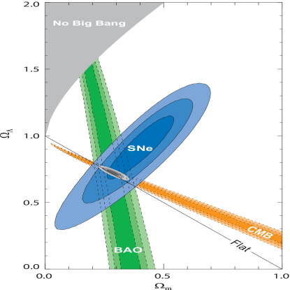
Figure 5: Constraints (68%, 95% and 99% CL contours) in the $(\Omega_{{\rm m}0},\Omega_{\Lambda 0})$ plane from SNIa, BAO and CMB. (From KowRubAld08.)

Further important input comes from weak lensing. The images of distant sources are distorted by the light-bending due to matter nearer to us. This distortion may be strong, for example causing multiple images of a single lensed galaxy, if the light passes very close to the lensing object, but for many cases only distorts what would be a circle into an ellipse: typically the ellipticity only changes by about 1%. We do not know the actual shape of the lensed object. Nevertheless, statistically one can extract the density distribution of the mass causing the lensing. The first map of dark matter using weak lensing (with a nice three-dimensional picture) was given by MasRhoEll07, in a 1.6 square degree area. The more recent data, with a method complementary to the statistical calculations [VanBenErb13], shows detailed maps of the (dark and visible) matter in regions several degrees across. Several lensing surveys are in progress to improve this data to the level where it may also be able to give additional information on dark energy. Lensing has also been detected in the CMB measurements [AdeAkiAnt14].

5.2 The standard model and the development of structure

The current standard model of cosmology is an expanding approximately FLRW Big Bang model, with, taking the values given by the Planck data [AdeAghArm14], $\Omega_{m}\approx 0.31$, of which about 0.05 is baryonic matter and the rest dark matter, and $\Omega_{\Lambda}\approx 0.69$. It is thus known as the $\Lambda$CDM model. These $\Omega$ values do not require revision of our understanding of thermal history, since $\Omega_{\Lambda}\ll\Omega_{m}$ for $z>1$. In the early universe, the standard model undergoes a period of inflation, with a rapid expansion driven by an inflaton, a field not (so far) observed terrestrially: exact details are model dependent. The crucial role of this early period is that it leads to a spectrum of classical density perturbations that is almost flat. The inflaton is typically modeled using a scalar field. This can give rise to a range of behaviours for $a(t)$ depending on $V(\phi)$. The thermal history of this model is described in Dur15 and will not be repeated here: it includes the nucleogenesis and other processes on which expansion exerts a major influence as described above. The development from the initial fluctuations to the last scattering surface and later times is modelled by perturbations of the FLRW background. This simple statement hides two problems, the choice of the FLRW model to perturb (the “fitting problem”), and the “gauge” issue which arises from the lack of an invariantly-defined map between the real lumpy Universe $M$ and the fictitious smooth FLRW universe $M^{\prime}$. The gauge issue is often described in coordinate terms, and then results in changes of variables similar to those of gauge transformations in field theory: hence the name. It is usual to identify points $p\in M$ and $p^{\prime}\in M^{\prime}$ which have the same coordinates, say $x^{a}=x^{\prime a}$. Making the same coordinate change in each manifold does not change this identification. If one slightly alters the map, i.e. the choice of $p^{\prime}$ for a given $p$, this can be described as mapping $x^{\prime a}$ to $x^{a}=x^{\prime a}+\delta x^{a}$, a change of gauge. Since this is clearly not a physical change in the real universe, one wants a description independent of the gauge choice. SteWal74 showed that the only gauge invariant quantities are those which in the background are zero, constant scalars, or sums of multiples of the tensor $\delta^{i}_{j}$. This is a nuisance, and in particular implies that there is no gauge-invariant way to define the perturbation of density in an FLRW model, since density is a time-dependent scalar. The fitting problem of picking the best-fit FLRW model for the comparison also involves gauge. The perturbed model could, for example, have greater average density than the initial model and so demand a different best fit. Fitting is also closely related to the “averaging problem” which is as follows. The equations (2)-(3) are nonlinear, and hence the averaged curvature is not the curvature of the averaged metric or averaged connection (because the average of a product, $<ab>$ say, is not the product of the averages $<a><b>$). This implies that the averaged density of the real universe may not be the same as that implied by (6) for the FLRW model whose average $H$ agrees with that of the real universe. One can try to estimate the effect by calculating the difference between the average of the curvature and the curvature of the averaged metric, the “backreaction”. Unfortunately we do not yet have a generally-agreed way to do this. The technical difficulties include the need to compare tensorial quantities at separated points, and the necessity of defining averaging volumes in a non-covariant way (since Lorentz transformations map a point at a finite distance to points on a hyperbola stretching to infinity). The various attempts are reviewed by [chapter 8]Kra97 and [chapter 16]EllMaaMac12, q.v. A further difficulty is that a best-fit RW metric (i.e. of form (4)) might not show the time evolution of an FLRW model with reasonable matter content. One approach much explored, because only averaging of scalars is required and this is well-defined, is that of Buchert: it involves averaging for fundamental observers and the non-commutation of the time derivative and averaging operators, leading to modified Friedman and Raychaudhuri equations (see e.g. Buc08). Because tensorial quantities are not averaged, this approach has to be completed by adding physical closure conditions. There are two main approaches to calculating the behaviour of perturbations, the metric-based method of Bar80 which develops the ideas of Lif46 into a gauge-invariant treatment, and the covariant approach of EllBru89 which developed ideas of Haw66. There are quite a large number of papers where these are expounded and applied: these are surveyed and summarized in [chapter 10]EllMaaMac12. A proper exposition is too lengthy to include here: I shall mention only the significance of expansion in the results. The role of the expansion rate in the evolution of perturbations arises because when perturbations have a length scale much greater than the contemporaneous Hubble scale, $c/H$, they are “frozen in”. This allows long wavelength perturbations to be tracked readily through the transitions from inflation through radiation domination to matter domination. (The Hubble scale has often been referred to in this context as the Hubble horizon, although it does not agree with any causal horizon. In a Big Bang the particle horizon at time $t_{o}$ is at comoving radial coordinate distance

$$u=\int_{0}^{t_{o}}\frac{{\mbox{\rm d}}t}{a(t)}$$

which in the de Sitter metric in its expanding form, (9), is bounded above by $1/H$. Although (9) is not really a Big Bang model, since it contains no matter, it appeared as the approximate metric for the early universe in the initial models of inflation, and this may be why the Hubble scale became called a horizon.) As discussed in Dur15, while the baryons and photons are tightly coupled the whole content undergoes acoustic oscillations under the competing effects of gravitational collapse and radiation pressure. These resulting waves travel at the sound speed of this medium, but become frozen in at decoupling, whence the peaks and troughs observed in the CMB power spectrum. The perturbation theory gives excellent agreement with the CMB fluctuations, but those observations only test scales above 150 Mpc. It is clear that nonlinear effects become important at smaller scales. Theories of galaxy formation and early evolution begin with collapse of a gas cloud, like star formation only larger, and then proceed by accretion and merger. The many theoretical inputs have been tabulated by Sco11. The main tool used to investigate the nonlinear phase of structure formation, beyond nonlinear perturbation theory, is large Newtonian N-body simulations. These can produce the principal features of the actual distributions of galaxies, walls, filaments, voids etc. However, they are not in perfect agreement with observation quantitatively and have a shaky theoretical basis, since they are non-relativistic. Their results do, for example, agree with the relativistic perturbation theory of FLRW models in the conformal Newtonian gauge [ChiZal11], but a recent paper has discussed a situation where inhomogeneities that are “easy to describe using the linearized general relativity” lead to a model that “taken as a whole lies in fact in the nonlinear regime” [Kor14]. In a $\Lambda$CDM model, the first structures to form are small, suggesting that massive galaxies form by multiple mergers. It is possible to use a “fossil record” of space- and time-resolved star formation histories, and so show that massive galaxies grow their mass from the inside out. The spheroidal parts seem to grow mainly about 5-7 Gyr ago. Earlier galaxies do not have the typical virialized structures we see today (ellipticals or spirals) and have now been seen (using the Hubble Space Telescope) to undergo the mergers expected. Each merger appears to take about 0.5 Gyr and a massive galaxy will have undergone 4-5 by today. There is growing evidence of correlations between the masses and sizes of galaxies (in particular their spheroidal parts) and the masses of their central supermassive black holes (SMBH); see for example KorHo13. How the SMBH controls the growth of a galaxy, given that it is typically only a thousandth of the total mass, is not yet entirely clear: it may be via the jets produced by the SMBH, fuelled by matter from an accretion disk, heating the surrounding gas and so controlling its collapse. What is clear is that this is highly nonlinear and another important cosmological application of general relativity.

5.3 Other models

Models other than FLRW can provide important cosmological information in several ways. They test whether features of FLRW models are peculiar to those models, and whether the models are robust under perturbations of parameters, and they admit a wide variety of potentially observable new effects. They may allow the nonlinear modelling of structures at a level which FLRW perturbation theory cannot address. The spatially homogeneous but anisotropic models, especially the expanding Big Bang cases, were extensively investigated from the 1960s onwards. They can be classified into the Bianchi types by their symmetry groups. The singularities that occur can be quite complicated, showing the oscillatory behaviour found by Mis69, and the more recently discovered “Mussel attractor” [ColHer05]. Over time, good choices of variables have been found for the systems of ordinary differential equations that arise, enabling very detailed and full studies [WaiEll97, EllMaaMac12]. Most of the dynamics can be understood qualitatively by patching together segments of the evolutions of the Bianchi I and II examples. Two areas of particular interest have been the approach to the singularity and the behaviour as $t\rightarrow\infty$. These are relevant to our understanding of the real Universe inasmuch as there are Bianchi models arbitrarily close to FLRW models for any given accuracy of approximation and length of time, and those models can differ radically from FLRW models at early and late times. However, a positive cosmological constant tends to isotropize all Bianchi models as $t\rightarrow\infty$ [Wal83]. Nucleosynthesis, the CMB observations, inflation, horizons and various quantum gravity theories have also been studied in Bianchi models. Among inhomogeneous models, the LTB models, the more general spherically symmetric models which were also first considered by Lemaître, and the Szekeres models [Sze75], have been the most extensively explored. Inhomogeneous spacetimes can model over- and under-densities, nonlinear gravitational waves, and anisotropic and inhomogeneous initial conditions, and some fit the SN1a and CMB data surprisingly well (for examples, see [chapter 19]EllMaaMac12), showing one should not too readily adopt the FLRW explanations. Inhomogeneities may help explain the apparent acceleration, as described below, but they also provide ways of making detailed nonlinear models of localized structures, such as the Local Group, M87, the Great Attractor and so on [BolKraHel10]. In modeling voids and clusters, it was found that velocity perturbations were more effective in producing structure than the usual density perturbations alone. It is sometimes said that inflation can explain the observed homogeneity and isotropy, despite the fact that almost all inflationary models start by assuming it, at least for the observable region. Calculations in specific models (summarized in [chapters 18–19]EllMaaMac12) suggest this is not so, and more needs to be done by combining non-FLRW geometries and varying forms of inflation to determine the true position. So far it seems that anisotropy and inhomogeneity may suppress inflation, though there is also a model in which averaged inhomogeneities act as the inflaton [BucOba11].

6 Open questions, and possible future developments

The standard model as we now have it has three big obvious unknowns in the natures of the inflaton, the dark matter and the dark energy. There are a number of terrestrial dark matter searches in progress and it is possible one of them will resolve that issue. I do not know of current experiments that could lead us to a fuller understanding of the inflaton: one would like to know in more detail how it governs the early universe dynamics and the generation of fluctuations, and the interactions by which its energy-momentum is converted to present-day matter. For the apparent acceleration of the expansion, a number of possible explanations have been put forward. While there may be astrophysical effects requiring amendment of our calibrations of the supernovae, and our understanding of absorption between them and us, which could alter the inferred $m-z$ relation, this seems increasingly unlikely as other, albeit still model-dependent, evidence for acceleration (from BAO or gamma ray bursters, for example) accumulates. Confidence in FLRW models, in which the various ways to define acceleration [BolAnd08] agree due to the symmetry, thus leads to some form of dark energy being necessary. There are four possible causes of the apparent acceleration other than the simple cosmological constant currently used in modeling. One is a previously unknown quantum field (“quintessence”) with some time dependence: observations currently under way aim at limiting the possible time development of such fields (assuming an FLRW model). Both large and small scale anisotropies might provide explanations, the former by using a non-FLRW geometry and the latter both by effects on light propagation and by the backreaction. Lastly, since the inferences depend on the relativistic FLRW models, a modified gravity theory may be indicated. Of these the most popular explanations are the first and last. Small scale anisotropies do affect measurements of $m-z$ both by their effect on light propagation and by the backreaction corrections to (6). However, the effects on light propagation, e.g. on galaxy number counts [BerMaaCla14], are probably only at the levels of accuracy claimed by “precision cosmology” [EllMaaMac12, chapter 15]. The possible models of backreaction by small scale inhomogeneities were put in doubt by the work of GreWal11, but may still provide a possible, and to me appealing, explanation of the apparent acceleration [RouOstBuc13, Kor14]. Large scale inhomogeneities could lead to an apparent acceleration. Since observations cannot directly separate spatial from temporal variations, a spatial variation could account for the observations, and a number of models on these lines have been devised (see [chapter 15]EllMaaMac12 for a review). However, it is not easy to fit all the phenomena, especially those which combine data from various $z$. For example, BulCliFer12 show that LTB models cannot simultaneously explain the SN1a results, the BAO, the local value of $H$ and the kinematic Sunyaev-Zel’dovich effect that arises (see Bir99) when the observed galaxies are in motion relative to a frame in which the CMB is isotropic. There are a great many projects under way to refine the present data from the CMB, SN1a, BAO, lensing, kinematic Sunyaev-Zeldovich effect, and other sources already described above. For example, there are at least 9 aimed at constraining the equation of state of dark energy (is it the $w=-1$ of the cosmological constant?), there are a number of experiments aimed at measuring B-mode polarizations and there are several terrestrial dark matter searches. Most of these involve very delicate measurement: for example, a 10% difference in $w$ from $-1$ implies a change of only 0.04 magnitudes in an SN1a at $z=0.6$. One further new window related to general relativity may be provided by gravitational waves (see the remarks in Dur15 on the BICEP2 results). The best current evidence for the existence of such waves is provided by the very detailed measurements of the binary and double pulsars, where the period changes agree well with the expected energy loss through gravitational radiation. In the near future, the ground-based laser interferometric detectors, with their recently improved sensitivity, will give interesting results whether they make a detection or not. (Since the predicted emission of expected sources should be detectable, not seeing anything would cause a re-evaluation of our theoretical understanding.) Pulsar timing arrays [McL14] are developing to the point of being very effective ways to detect low frequency waves. There is still hope that the space-based interferometric detector LISA will fly within some of the readers’ lifetimes. In the seminar I referred to in the introduction, Sciama explained how the 1960s data favoured the Big Bang theory, and described the relevant FLRW models. We now have a great deal more than one known piece of cosmological data, though it is perhaps disappointing that that piece, i.e. the value of $H$, is still rather imprecisely known, as the divergent values at the end of section 3 show. Even more can be confidently anticipated. However, it is far from clear whether or when the big open questions just mentioned will be settled. It could even be that evidence emerges forcing us to replace general relativistic dynamics for the Universe. What seems likely is that expansion will continue to play a big role in our models.

References

References

- [1] \harvarditemAde et al.2014AdeAkiAnt14 Ade P A R et al. 2014 Astrophys. J. 794, 171.
- [2] \harvarditemAde et al.2014AdeAghArm14 Ade P A R et al. 2014 Astron. Astrophys. 571, A16.
- [3] \harvarditemAlpher et al.1953AlpFolHer53 Alpher R A, Follin J W \harvardand Herman R C 1953 Phys. Rev. 92, 1347–1361.
- [4] \harvarditemAlpher \harvardand Herman1949AlpHer49 Alpher R A \harvardand Herman R C 1949 Phys. Rev. 75, 1089–1095.
- [5] \harvarditemBardeen1980Bar80 Bardeen J M 1980 Phys. Rev. D 22, 1882–1905.
- [6] \harvarditemBarrow1976Bar76 Barrow J D 1976 Mon. Not. Roy. Astr. Soc. 175, 359.
- [7] \harvarditemBatchelor1967Bat67 Batchelor G K 1967 An introduction to fluid dynamics Cambridge University Press Cambridge.
- [8] \harvarditemBelinskii et al.1982BelKhaLif82 Belinskii V, Khalatnikov I M \harvardand Lifshitz E M 1982 Advances Phys. 31, 639–67.
- [9] \harvarditemBertacca et al.2014BerMaaCla14 Bertacca D, Maartens R \harvardand Clarkson C 2014 J. Cosm. Astroparticle Phys. 11, 013.
- [10] \harvarditemBessell2005Bes05 Bessell M S 2005 Annual Review of Astronomy and Astrophysics 43, 293–336.
- [11] \harvarditemBirkinshaw1999Bir99 Birkinshaw M 1999 Phys. Reports 310, 97.
- [12] \harvarditemBlake et al.2011BlaKazBeu11 Blake C et al. 2011 Mon. Not. Roy. Astr. Soc. 418, 1707–1724.
- [13] \harvarditemBolejko \harvardand Andersson2008BolAnd08 Bolejko K \harvardand Andersson L 2008 J. Cosm. Astroparticle Phys. 10/2008, 003.
- [14] \harvarditemBolejko et al.2010BolKraHel10 Bolejko K, Krasiński A, Hellaby C \harvardand Célérier M N 2010 Structures in the Universe by exact methods: formation, evolution, interactions Cambridge University Press Cambridge.
- [15] \harvarditemBond et al.2013BonNelVan13 Bond H E et al. 2013 Astrophys. J. Lett. 765, L12.
- [16] \harvarditemBondi1960Bon60 Bondi H 1960 Cosmology Cambridge University Press Cambridge.
- [17] \harvarditemBondi \harvardand Gold1948BonGol48 Bondi H \harvardand Gold T 1948 Mon. Not. Roy. Astr. Soc. 108, 252–270.
- [18] \harvarditemBonnor1956Bon56 Bonnor W B 1956 Z. Astrophys. 39, 143. Reprinted, with commentary by A. Krasiński and autobiography, in Gen. Rel. Grav. 30 1113-1132 1998.
- [19] \harvarditemBuchert2008Buc08 Buchert T 2008 Gen. Relativ. Gravit. 40, 467–527.
- [20] \harvarditemBuchert et al.2006BucLarAli06 Buchert T, Larena J \harvardand Alimi J M 2006 Class. Quantum Grav. 23, 6379–6408.
- [21] \harvarditemBuchert \harvardand Obadia2011BucOba11 Buchert T \harvardand Obadia N 2011 Class. Quantum Grav. 28, 162002.
- [22] \harvarditemBull et al.2012BulCliFer12 Bull P, Clifton T \harvardand Ferreira P G 2012 Phys. Rev. D 85, 024002.
- [23] \harvarditemBurbidge et al.1957BurBurFow57 Burbidge E M, Burbidge G, Fowler W A \harvardand Hoyle F 1957 Rev. Mod. Phys. 29, 547–650.
- [24] \harvarditemChisari \harvardand Zaldarriaga2011ChiZal11 Chisari N E \harvardand Zaldarriaga M 2011 Phys. Rev. D 83, 123505. Erratum Phys. Rev. D 84, 089901 (2011).
- [25] \harvarditemChristianson1995Chr95 Christianson G E 1995 Edwin Hubble: mariner of the nebulae Institute of Physics Publishing London and Bristol.
- [26] \harvarditemColes \harvardand Ellis1997ColEll97 Coles P \harvardand Ellis G F R 1997 Is the Universe open or closed? The density of matter in the Universe Vol. 7 of Cambridge Lecture Notes in Physics Cambridge University Press Cambridge.
- [27] \harvarditemColey \harvardand Hervik2005ColHer05 Coley A A \harvardand Hervik S 2005 Class. Quantum Grav. 22, 579–606.
- [28] \harvarditemColey \harvardand Tupper1983ColTup83 Coley A A \harvardand Tupper B O J 1983 Gen. Relativ. Gravit. 15, 977.
- [29] \harvarditemCyburt et al.2005CybFieOli05 Cyburt R H, Fields B D, Olive K A \harvardand Skillman E 2005 Astropart. Phys. 23, 313–323.
- [30] \harvarditemde Bruijne et al.2001deHoode01 de Bruijne J H J, Hoogerwerf R \harvardand de Zeeuw P T 2001 Astron. Astrophys. 367, 111–147.
- [31] \harvarditemde Sitter1917ade17a de Sitter W 1917a Proc. Kon. Ned. Akad. Wet. 20, 229–243. Available from http://www.dwc.knaw.nl/toegangen/digital-library-knaw/?pagetype=bundel.
- [32] \harvarditemde Sitter1917bde17 de Sitter W 1917b Proc. Kon. Ned. Akad. Wet. 19, 1217–1225. Available from http://www.dwc.knaw.nl/toegangen/digital-library-knaw/?pagetype=bundel.
- [33] \harvarditemDelubac et al.2015DelBauBus15 Delubac T et al. 2015 Astron. Astrophys. 574, A59.
- [34] \harvarditemDoroshkevich \harvardand Novikov1964DorNov64 Doroshkevich A G \harvardand Novikov I D 1964 Sov. Phys. Doklady 9, 111. Translation of Dokl. Akad. Nauk U.S.S.R. 154, 809 (1964).
- [35] \harvarditemDurrer2015Dur15 Durrer R 2015 Class. Quantum Grav. 32. Milestone preprint. To appear.
- [36] \harvarditemDyer \harvardand Roeder1974DyeRoe74 Dyer C C \harvardand Roeder R 1974 Astrophys. J. 189, 167.
- [37] \harvarditemEckart \harvardand Genzel1996EckGen96 Eckart A \harvardand Genzel R 1996 Nature 383, 415.
- [38] \harvarditemEddington1923Edd23 Eddington A S 1923 The mathematical theory of relativity Cambridge University Press Cambridge.
- [39] \harvarditemEddington1926Edd26 Eddington A S 1926 The internal constitution of the stars Cambridge University Press Cambridge. Reissued in the Cambridge Science Classics series, 1988.
- [40] \harvarditemEddington1930Edd30 Eddington A S 1930 Mon. Not. Roy. Astr. Soc. 90, 668–678.
- [41] \harvarditemEfstathiou et al.1990EfsSutMad90 Efstathiou G, Sutherland W J \harvardand Maddox S J 1990 Nature 348, 705–707.
- [42] \harvarditemEhlers2009Ehl09 Ehlers J 2009 Gen. Relativ. Gravit. 41, 1655–1660.
- [43] \harvarditemEinstein1915Ein15 Einstein A 1915 Preuss. Akad. Wiss., Sitzungsberichte (part 2) pp. 844–847.
- [44] \harvarditemEinstein1917Ein17 Einstein A 1917 Sitzb. Preuss. Akad. Wiss. pp. 142–152. English translation in ‘The Principle of Relativity’ by H. A. Lorentz, A. Einstein, H. Minkowski and H. Weyl, pp. 175-188 (Methuen, London, 1923, reprinted by Dover, New York, 1952).
- [45] \harvarditemEinstein1931Ein31 Einstein A 1931 Preuss. Akad. Wiss., Sitzb. 12, 235–237.
- [46] \harvarditemEinstein \harvardand de Sitter1932Einde32 Einstein A \harvardand de Sitter W 1932 Proc. Nat. Acad. Sci. U.S. 18, 213.
- [47] \harvarditemEllis1971Ell71 Ellis G F R 1971 in R Sachs, ed., ‘General relativity and cosmology. Proceedings of the International school of Physics ”Enrico Fermi”’ Vol. XLVII Academic Press New York and London pp. 104–182. Reprinted as Gen. Rel. Grav. 41, 581-660 (2009).
- [48] \harvarditemEllis1989Ell89 Ellis G F R 1989 in D Howard \harvardand J Stachel, eds, ‘Einstein and the History of general relativity’ Vol. 1 of Einstein Study Series Birkhauser Boston pp. 367–431.
- [49] \harvarditemEllis \harvardand Bruni1989EllBru89 Ellis G F R \harvardand Bruni M 1989 Phys. Rev. D 40, 1804–1818.
- [50] \harvarditemEllis \harvardand Hawking1968EllHaw68 Ellis G F R \harvardand Hawking S W 1968 Astrophys. J. 152, 25.
- [51] \harvarditemEllis et al.2012EllMaaMac12 Ellis G F R, Maartens R \harvardand MacCallum M A H 2012 Relativistic cosmology Cambridge University Press Cambridge.
- [52] \harvarditemEllis et al.1978EllMaaNel78 Ellis G F R, Maartens R \harvardand Nel S D 1978 Mon. Not. Roy. Astr. Soc. 184, 439.
- [53] \harvarditemEllis et al.2013EllMcLDun13 Ellis R S et al. 2013 Astrophys. J. Lett. 763, L7.
- [54] \harvarditemField et al.1973FieArpBah73 Field G B, Arp H \harvardand Bahcall J N 1973 The redshift controversy W.A. Benjamin New York.
- [55] \harvarditemFriedman1922Fri22 Friedman A 1922 Z. Phys. 31, 1991–2000.
- [56] \harvarditemFriedman1999Fri99 Friedman A 1999 Gen. Relativ. Gravit. 31, 1985–2008. Papers translated by G. F. R. Ellis and H. van Elst and accompanied by an editorial note by A. Krasiński and G. F. R. Ellis.
- [57] \harvarditemFriedmann1924Fri24 Friedmann A 1924 Z. Phys. 31, 2001–08.
- [58] \harvarditemGamow1946Gam46 Gamow G 1946 Phys. Rev. 70, 572–573.
- [59] \harvarditemGamow1948Gam48 Gamow G 1948 Phys. Rev. 74, 505–506.
- [60] \harvarditemGamow1956Gam56 Gamow G 1956 Sci. Amer. (Sept), 136–154.
- [61] \harvarditemGhez et al.2008GheSalWei08 Ghez A M et al. 2008 Astrophys. J. 689, 1044.
- [62] \harvarditemGreen \harvardand Wald2011GreWal11 Green S R \harvardand Wald R M 2011 Phys. Rev. D 83, 084020.
- [63] \harvarditemHarrison1973Har73 Harrison E R 1973 in E Schatzman, ed., ‘Cargése Lectures in Physics, vol.6’ Gordon and Breach New York pp. 581–641.
- [64] \harvarditemHarrison1981Har81 Harrison E R 1981 Cosmology : the science of the universe (second edition) Cambridge University Press Cambridge. Also second edition (2000).
- [65] \harvarditemHawking1966Haw66 Hawking S W 1966 Astrophys. J. 145, 544–554.
- [66] \harvarditemHawking \harvardand Ellis1973HawEll73 Hawking S W \harvardand Ellis G F R 1973 The large scale structure of space-time Cambridge Univ. Press Cambridge.
- [67] \harvarditemHayashi1950Hay50 Hayashi C 1950 Prog. Theor. Phys. 5, 224–245.
- [68] \harvarditemHeller1974Hel74 Heller M 1974 Acta Cosmologica 2, 37–41.
- [69] \harvarditemHetherington1972Het72 Hetherington N S 1972 Quart. J. Roy. Astr. Soc. 13, 25–39.
- [70] \harvarditemHoyle1948Hoy48 Hoyle F 1948 Mon. Not. Roy. Astr. Soc. 108, 372–382.
- [71] \harvarditemHubble1925aHub25a Hubble E P 1925a The Observatory 48, 139–142.
- [72] \harvarditemHubble1925bHub25 Hubble E P 1925b Astrophys. J. 62, 409–433.
- [73] \harvarditemHubble1926Hub26 Hubble E P 1926 Astrophys. J. 64, 321.
- [74] \harvarditemHubble1929Hub29 Hubble E P 1929 Proc. Nat. Acad. Sci. U.S. 15, 168–173.
- [75] \harvarditemHubble1936Hub36 Hubble E P 1936 Astrophys. J. 84, 517–554.
- [76] \harvarditemHubble1938Hub38 Hubble E P 1938 The observational approach to cosmology Oxford University Press Oxford.
- [77] \harvarditemHubble1953Hub53 Hubble E P 1953 Mon. Not. Roy. Astr. Soc. 113, 658–666.
- [78] \harvarditemKaiser2014Kai14 Kaiser N 2014 Mon. Not. Roy. Astr. Soc. 438, 2456–2465.
- [79] \harvarditemKapteyn1922Kap22 Kapteyn J C 1922 Astrophys. J. 55, 302.
- [80] \harvarditemKing et al.2012KinWebMur12 King J A et al. 2012 Mon. Not. Roy. Astr. Soc. 422, 3370–3414.
- [81] \harvarditemKormendy \harvardand Ho2013KorHo13 Kormendy J \harvardand Ho L 2013 Ann. Rev. Astron. Astrophys. 5, 511–653.
- [82] \harvarditemKorzyński2014Kor14 Korzyński M 2014. Nonlinear effects of general relativity from multiscale structure arXiv:1412.3865.
- [83] \harvarditemKowalski et al.2008KowRubAld08 Kowalski M et al. 2008 Astrophys. J. 686, 749–778.
- [84] \harvarditemKramer et al.1980KraSteMac80 Kramer D, Stephani H, MacCallum M A H \harvardand Herlt E 1980 Exact solutions of Einstein’s field equations Deutscher Verlag der Wissenschaften, Berlin, and Cambridge University Press Cambridge.
- [85] \harvarditemKrasiński1997Kra97 Krasiński A 1997 Inhomogeneous cosmological models Cambridge University Press Cambridge.
- [86] \harvarditemKristian \harvardand Sachs1966KriSac66 Kristian J \harvardand Sachs R K 1966 Astrophys. J. 143, 379–399. Reprinted, with editorial note by G. F.R. Ellis and biographical notes by A. Krasiński, in Gen. Rel. Grav. 43 331-58 (2011).
- [87] \harvarditemLandau \harvardand Lifshitz1941LanLif41 Landau L D \harvardand Lifshitz E M 1941 The classical theory of fields Gostekhizdat Moscow. First English edition: Addison-Wesley, Cambridge, Mass. (1951).
- [88] \harvarditemLehnert et al.2010LehNesCub10 Lehnert M D et al. 2010 Nature 467, 940–942.
- [89] \harvarditemLemaître1927Lem27 Lemaître G 1927 Ann. Soc. Sci. Bruxelles A 47, 49–59. Translated and republished in 1931 as Mon. Not. Roy. Astr. Soc., 41, 483-490. See also Lemaître 2013.
- [90] \harvarditemLemaître1931Lem31 Lemaître G 1931 Nature 127, 706. Reprinted as Gen. Rel. Grav. 43, 2929-30 (2011) with editorial note by J.-P. Luminet.
- [91] \harvarditemLemaître1933Lem33 Lemaître G 1933 Ann. Soc. Sci. Bruxelles A 53, 51. Translated by M.A.H. MacCallum and republished with commentary by A. Krasiński as Gen. Rel. Grav. 29, 641-680 1997.
- [92] \harvarditemLemaître2013Lem13 Lemaître G 2013 GRG 45, 1619–46. Reprint of Lemaître 1927, translated by and with editorial note (pp. 1619-33) by J.-P. Luminet.
- [93] \harvarditemLifshitz1946Lif46 Lifshitz E M 1946 Acad. Sci. USSR J. Phys. 10, 116.
- [94] \harvarditemLindblad1927Lin27 Lindblad B 1927 Mon. Not. Roy. Astr. Soc. 87, 553–564.
- [95] \harvarditemLivio2011Liv11 Livio M 2011 Nature 479, 171–173.
- [96] \harvarditemLongair \harvardand Rees1973LonRee73 Longair M S \harvardand Rees M J 1973 in E Schatzman, ed., ‘Cargése Lectures in Physics, vol.6’ Gordon and Breach New York pp. 269–400.
- [97] \harvarditemLundmark1919Lun19 Lundmark K 1919 Astron. Nachr. 209, 369.
- [98] \harvarditemLundmark1924Lun24 Lundmark K 1924 Mon. Not. Roy. Astr. Soc. 84, 747.
- [99] \harvarditemLynden-Bell et al.1988LynFabBur88 Lynden-Bell D et al. 1988 Astrophys. J. 326, 19.
- [100] \harvarditemMacCallum \harvardand Ellis1970MacEll70 MacCallum M A H \harvardand Ellis G F R 1970 Commun. math. phys. 19, 31–64.
- [101] \harvarditemMariano \harvardand Perivolaropoulos2013MarPer13 Mariano A \harvardand Perivolaropoulos L 2013 Phys. Rev. D 87, 043511.
- [102] \harvarditemMassey et al.2007MasRhoEll07 Massey R et al. 2007 Nature 445, 286–290.
- [103] \harvarditemMcArthur et al.2011McABenHar11 McArthur B E, Benedict G F, Harrison T E \harvardand van Altena W 2011 Astron. J. 141, 172.
- [104] \harvarditemMcLaughlin2014McL14 McLaughlin M 2014 Gen. Relativ. Gravit. 46, 1810. Plenary lecture at the GR20 conference.
- [105] \harvarditemMisner1969Mis69 Misner C W 1969 Phys. Rev. Lett. 22, 1071–1074.
- [106] \harvarditemMurphy et al.2003MurWebFla03 Murphy M T, Webb J K \harvardand Flambaum V V 2003 Mon. Not. Roy. Astr. Soc. 345, 609.
- [107] \harvarditemNorth1965Nor65 North J D 1965 The measure of the universe Oxford University Press Oxford. Re-issued by Dover, New York, 1990 with new preface.
- [108] \harvarditemNovikov2009Nov09 Novikov I D 2009 in P. J. E Peebles, L. A Page, Jr. \harvardand R. B Partridge, eds, ‘Finding the Big Bang’ Cambridge University Press Cambridge pp. 99–106.
- [109] \harvarditemNugent et al.2011NugSulCen11 Nugent P E et al. 2011 Nature 480, 344–347.
- [110] \harvarditemOort1927Oor27 Oort J H 1927 Bull. Astron. Inst. Neth. 3, 275.
- [111] \harvarditemOort et al.1924OorAriRoj24 Oort J H, Arias B, Rojo M \harvardand Massa M 1924 Proc Natl Acad Sci U S A. 10(6), 256––260.
- [112] \harvarditemO’Raifeartaigh \harvardand McCann2014ORaMcC14 O’Raifeartaigh C \harvardand McCann B 2014 Eur. J. Phys. H 39, 63.
- [113] \harvarditemOstriker \harvardand Steinhardt1995OstSte95 Ostriker J P \harvardand Steinhardt P J 1995 Nature 377, 600–602.
- [114] \harvarditemPeacock2013Pea13 Peacock J A 2013 in M. J Way \harvardand D Hunter, eds, ‘Origins of the Expanding Universe: 1912-1932 Proceedings of a conference held 13-15 September, 2012, at Flagstaff, Arizona, USA’ Vol. 471 of ASP Conference Proceedings Astronomical Society of the Pacific San Francisco p. 3.
- [115] \harvarditemPooley \harvardand Ryle1968PooRyl68 Pooley G G \harvardand Ryle M 1968 Mon. Not. Roy. Astr. Soc. 139, 515–528.
- [116] \harvarditemRees \harvardand Sciama1968ReeSci68 Rees M J \harvardand Sciama D W 1968 Nature 217, 511–516.
- [117] \harvarditemRiess et al.2011RieMacCas11 Riess A G et al. 2011 Astrophys. J. 730, 119.
- [118] \harvarditemRobertson1929Rob29 Robertson H P 1929 Proc. Nat. Acad. Sci. U.S. 15, 822–829.
- [119] \harvarditemRobertson1933Rob33 Robertson H P 1933 Rev. Mod. Phys. 5, 62–90. Reprinted as Gen. Rel. Grav. 44 2115-44 (2012) with editorial note by G. F.R. Ellis and biography by A. Krasiński.
- [120] \harvarditemRobertson1935Rob35 Robertson H P 1935 Astrophys. J. 82, 284.
- [121] \harvarditemRobertson1936Rob36 Robertson H P 1936 Astrophys. J. 83, 187.
- [122] \harvarditemRoukema et al.2015RouBucOst15 Roukema B F, Buchert T \harvardand Ostrowski J J 2015 Mon. Not. Roy. Astr. Soc. 448, 1660.
- [123] \harvarditemRoukema et al.2013RouOstBuc13 Roukema B F, Ostrowski J J \harvardand Buchert T 2013. Virialization-induced curvature versus dark energy arXiv:1311.5402.
- [124] \harvarditemRowan-Robinson1985Row85 Rowan-Robinson M 1985 The cosmic distance ladder W.H. Freeman New York.
- [125] \harvarditemSachs \harvardand Wolfe1967SacWol67 Sachs R K \harvardand Wolfe A M 1967 Astrophys. J. 147, 73. Republished, with commentary by G.F.R. Ellis and J. Ehlers, as Gen. Rel. Grav. 39 1944 (2007).
- [126] \harvarditemScott2011Sco11 Scott D 2011 Astron. & Geophys. 52, 6.31.
- [127] \harvarditemShapley1918Sha18 Shapley H 1918 Publ. Astr. Soc. Pacific 30, 42.
- [128] \harvarditemSlipher1913Sli13 Slipher V M 1913 Lowell Observatory Bulletin (58), 56.
- [129] \harvarditemSlipher1914Sli14 Slipher V M 1914 Lowell Observatory Bulletin 12(62).
- [130] \harvarditemSlipher1917Sli17 Slipher V M 1917 Proc. Amer. Phil. Soc 56, 403.
- [131] \harvarditemSteer2011Ste11 Steer I 2011 J. Roy. Astr. Soc. Canada 105(1), 18.
- [132] \harvarditemSteigman et al.1977SteSchGun77 Steigman G, Schramm D N \harvardand Gunn J E 1977 Phys. Lett. B 66, 202.
- [133] \harvarditemStephani et al.2003SteKraMac03 Stephani H et al. 2003 Exact solutions of Einstein’s field equations, 2nd edition Cambridge University Press Cambridge. Corrected Paperback edition, 2009.
- [134] \harvarditemStewart et al.1970SteMacSci70 Stewart J M, MacCallum M A H \harvardand Sciama D W 1970 Comments in Astrophys. and Space Phys. 2, 206–8.
- [135] \harvarditemStewart \harvardand Walker1974SteWal74 Stewart J M \harvardand Walker M 1974 Proc. Roy. Soc. London A 341, 49–74.
- [136] \harvarditemSunyaev \harvardand Zel’dovich1970SunZel70 Sunyaev R \harvardand Zel’dovich Y B 1970 Astrophys. Sp. Sci. 7, 3–19.
- [137] \harvarditemSzekeres1975Sze75 Szekeres P 1975 Commun. math. phys. 41, 55.
- [138] \harvarditemTipler et al.1980TipClaEll80 Tipler F J, Clarke C J S \harvardand Ellis G F R 1980 in A Held, ed., ‘General relativity and gravitation: one hundred years after the birth of Albert Einstein’ Vol. 2 Plenum New York p. 97.
- [139] \harvarditemTolman1934Tol34 Tolman R C 1934 Relativity, thermodynamics and cosmology Clarendon Press Oxford.
- [140] \harvarditemTrimble1995Tri95 Trimble V 1995 Publ. Astr. Soc. Pacific 107, 1133.
- [141] \harvarditemTrumpler1930aTru30 Trumpler R J 1930a Publ. Astr. Soc. Pacific 42, 214.
- [142] \harvarditemTrumpler1930bTru30a Trumpler R J 1930b Publ. Astr. Soc. Pacific 42, 267.
- [143] \harvarditemvan Maanen1916van16 van Maanen A 1916 Astrophys. J. 44, 201.
- [144] \harvarditemVan Waerbeke et al.2013VanBenErb13 Van Waerbeke L et al. 2013 Mon. Not. Roy. Astr. Soc. 433, 3373.
- [145] \harvarditemWagoner et al.1967WagFowHoy67 Wagoner R V, Fowler W A \harvardand Hoyle F 1967 Astrophys. J. 148, 3–50.
- [146] \harvarditemWainwright \harvardand Ellis (eds)1997WaiEll97 Wainwright J \harvardand Ellis (eds) G F R 1997 Dynamical systems in cosmology Cambridge University Press Cambridge.
- [147] \harvarditemWald1983Wal83 Wald R M 1983 Phys. Rev. D 28, 2118–20.
- [148] \harvarditemWalker1935Wal35 Walker A G 1935 Quart. J. Math. 6, 81–93.
- [149] \harvarditemWill2015Wil15 Will C M 2015 Class. Quantum Grav. 32. Milestone preprint. To appear.
- [150] \harvarditemZibin \harvardand Moss2014ZibMos14 Zibin J P \harvardand Moss A 2014. Nowhere to hide: closing in on cosmological homogeneity arXiv:1409.3831.
- [151]