Phase diagram and critical properties of Yukawa bilayers

Abstract

We study the ground-state Wigner bilayers of pointlike particles with Yukawa pairwise interactions, confined to the surface of two parallel hard walls at dimensionless distance $\eta$. The model involves as limiting cases the unscreened Coulomb potential and hard spheres. The phase diagram of Yukawa particles, studied numerically by Messina and Löwen [Phys. Rev. Lett. 91 (2003) 146101], exhibits five different staggered phases as $\eta$ varies from 0 to intermediate values. We present a lattice summation method using the generalized Misra functions which permits us to calculate the energy per particle of the phases with a precision much higher than usual in computer simulations. This allows us to address some tiny details of the phase diagram. Going from the hexagonal phase I to phase II is shown to occur at $\eta=0$, which resolves a longtime controversy. We find a tricritical point where Messina and Löwen suggested a coexistence domain of several phases which was suggested to divide the staggered rhombic phase into two separate regions. Our calculations reveal one continuous region for this rhombic phase with a very narrow connecting channel. Further we show that all second-order phase transitions are of mean-field type. We also derive the asymptotic shape of critical lines close to the Coulomb and hard-spheres limits. In and close to the hard-spheres limit, the dependence of the internal parameters of the present phases on $\eta$ is determined exactly.

I Introduction

Most organic or anorganic surfaces of mesoscopic objects (macromolecules or colloids) become charged when immersed in polar solvents such as water. These solvents provide favorable environments for free charges (“counter-ions” to the charged surfaces) which intermediate an effective interaction among the mesoscopic objects. At low temperatures, and in particular at $T=0$ when the system is in its ground state, counter-ions between two charged plates crystallize into bilayer Wigner structures which are important in understanding anomalous phenomena such as like-charge attraction or overcharging Lau ; Grosberg ; Levin ; Naji ; Samaj . Bilayer Wigner crystals describe several real physical systems in condensed and soft matter, such as semiconductors Fil , quantum dots Imamura and dusty plasmas Teng . Confined systems of charged colloidal particles were reviewed recently review , both from experimental and theoretical point of view.

From the particle models studied in this paper, we start with the neutral Coulomb system of say elementary pointlike charges $-e$ with $1/r$ interaction between two parallel plates of the same homogeneous surface charge density $\sigma e$ at distance $d$, the phase diagram at $T=0$ depends on a single dimensionless parameter $\eta=d\sqrt{\sigma}$. According to the Earnshaw theorem Earnshaw , particles will stick symmetrically on the surface of the plates. Five distinct phases were detected to be stable, i.e. providing global minimum of the energy, as $\eta$ is changing from 0 to $\infty$ Falko ; Esfarjani ; Goldoni ; Schweigert ; Weis . The lattice structures are the same on both plates and they are shifted laterally with respect to one another. Structures I, III and V are rigid (Fig. 1), i.e. they have fixed ($\eta$-independent) primary cells. Structures II and IV are soft (Fig. 2), the shape of their primary cells is varying with $\eta$.

Figure 1: Rigid structures I, III and V of particles on two parallel plates; open and filled symbols correspond to particle positions on the opposite layers.

Figure 2: Soft structures II and IV.

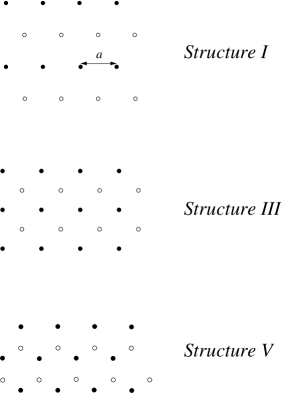
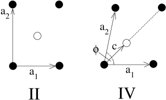
Structures I, II and III correspond to the staggered rectangular lattice, see Fig. 2 left. The primitive translation vectors of Bravais lattice are

$${\bm{a}}_{1}=a(1,0),\quad{\bm{a}}_{2}=a(0,\Delta),\quad a=\frac{1}{\sqrt{\sigma\Delta}}.$$ (1)

The lattice spacing $a$ within one layer is determined by the electroneutrality condition. Two rectangular structures, one within each layer, are shifted with respect to each other by the vector

$${\bm{c}}=\alpha({\bm{a}_{1}}+{\bm{a}_{2}})$$ (2)

with $\alpha=1/2$. The rigid structure I has the aspect ratio $\Delta=\sqrt{3}$ and it arises for $\eta=0$ because the two layers merge into a Wigner monolayer which is known to be hexagonal (or, equivalently, equilateral triangular) Bonsall77 . Structure III consists of a square lattice with $\Delta=1$. Phase II with $\sqrt{3}>\Delta>1$ interpolates continuously between structures I and III.

Phase IV consists of two staggered rhombus lattices (Fig. 2 right). One rhombus structure has the angle $\phi$ between the primitive translation vectors

$${\bm{a}}_{1}=a(1,0),\quad{\bm{a}}_{2}=a(\cos\phi,\sin\phi),\quad a=\frac{1}{\sqrt{\sigma\sin\phi}}.$$ (3)

In general, this phase has two variants according to the lateral shift (2) between the opposite sublattices. The version IVA has $\alpha=1/2$ whereas for IVB the shift parameter $1/3<\alpha<1/2$. For Coulomb bilayers, only phase IVA takes place.

Phase V corresponds to two shifted hexagonal lattices. In a single layer, the elementary cell is the rhombus with the primitive translation vectors

$${\bm{a}}_{1}=a(1,0),\quad{\bm{a}}_{2}=\frac{a}{2}(1,\sqrt{3}),\quad a=\frac{\sqrt{2}}{3^{1/4}\sqrt{\sigma}}.$$ (4)

The lateral shift between the opposite lattices ${\bm{c}}$ is given by (2) with $\alpha=1/3$.

The transitions between phases ${\rm II}\to{\rm III}$ and ${\rm III}\to{\rm IV}$ are continuous (of second order), while the transition ${\rm IV}\to{\rm V}$ is discontinuous (of first order). In order to describe these phase transitions, a new analytic approach to Coulomb bilayers was proposed in Ref. Samaj1 . Using a series of transformations with Jacobi theta functions, the energy of the five phases was expressed as series of generalized Misra functions which converge very quickly. Near critical points, the generalized Misra functions can be expanded easily in powers of the order parameter and the corresponding energies posses the Ginsburg-Landau form. This allows one to specify the critical points with an arbitrary prescribed accuracy and to derive the mean-field critical behavior of the order parameter. Also the existence of phase I at $\eta=0$ only was confirmed. This result was in contradiction with numerical approaches like Ewald technique Goldoni and Monte Carlo simulations Weis which predicted an extremely small, but finite, stability interval of $\eta$’s for phase I.

Colloidal particles or particles in highly charged dusty plasmas usually interact via Yukawa potential Nunomura due to the Coulomb potential screening by additional microions in the system. The Yukawa pair potential of particles at distance $r$ is defined by

$$V(r)=V_{0}\ \frac{{\rm e}^{-\kappa r}}{\kappa r},$$ (5)

where $\kappa$ is the inverse screening length and the amplitude $V_{0}=Z^{2}\kappa\exp{(\kappa R)}/\epsilon(1+\kappa R)^{2}$, with $Z$ being the charge of one particle and $\epsilon\approx\epsilon_{0}$ is the permittivity for dusty plasma. When $\kappa$ is large, $R$ becomes the radius of a hard sphere as $V(r)\propto\exp{[\kappa(R-r)]}$ is exponentially large for $r<R$ and negligible otherwise. The relation $V_{0}\propto\kappa$ keeps the limit $\kappa\to 0$ of Eq. (5) finite, yielding the proper Coulomb formula. Thus the limiting cases $\kappa\to 0$ and $\kappa\to\infty$ correspond to the unscreened Coulomb and hard-spheres interaction potentials, respectively. We shall work in units of $V_{0}=1$. For two parallel plates at distance $d$, the phase diagram depends on two dimensionless parameters

$$\eta=\sqrt{\sigma}d,\qquad\lambda=\kappa d.$$ (6)

A system of hard-sphere particles between two parallel hard plates was studied by computer simulations in the past Murray ; Schmidt ; Neser ; Fortini ; numerical methods were reviewed recently in Ref. Mazars11 . For small values of $\eta$, the ground-state crystal structures involve Wigner bilayers I-V, including phase IVB with two varying parameters $\phi$ and $\alpha$. For large values of $\eta$, phase-V bilayer transforms itself to crystalline multilayers, with particles entering the region between the plates, such as multiple square and hexagonal layers Murray , rhombic Schmidt and prism superlattices Neser .

A similar phase diagram was obtained for the general Yukawa potential. For small values of $\eta$, although Earnshaw theorem Earnshaw does not apply to Yukawa particles, the particles stick symmetrically to plates and with increasing $\eta$ they constitute successively Wigner I-V bilayers Messina . In the region of large values of $\eta$, in close analogy with confined hard spheres, some of the particles will move in the interior of the domain between the plates and create multilayers Oguz .

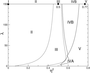
In this paper, we shall concentrate on Wigner bilayers of pointlike particles interacting via Yukawa potential. The original numerical work of Messina and Löwen Messina determined the phase diagram of the Yukawa system which exhibits single and double reentrant transition. We shall apply a straightforward extension of the recent analytic method Samaj1 which provides us with high precision calculations to shed more light on important tiny details of the phase diagram. For any $\lambda$, the transition from phase I to II is shown to occur directly at $\eta=0$, which solves a longtime controversy. We recall that this scenario was anticipated only in the hard-spheres limit $\lambda\to\infty$ Messina . We find a tricritical point where Messina and Löwen suggested a coexistence domain of several phases which should divide one staggered rhombic phase into two separate regions. Our calculations reveal one continuous region for this rhombic phase with a narrow connecting channel. Closed-form formulas for critical lines between various phases, expressed in terms of generalized Misra functions, permit us to determine the asymptotic Coulomb $\lambda\to 0$ and hard spheres $\lambda\to\infty$ shapes of these lines. The expansions of the structure energies around second-order transition points and the determination of the order parameter can be done analytically, which enables us to derive the critical behavior of the Ginzburg-Landau type. In and close to the hard-spheres limit, the $\eta$-dependence of the internal parameters of the phases is determined exactly.

The paper is organized as follows. In Sec. II, we derive the expression for the energy per particle of phase II (phases I and III being its special cases) in terms of the generalized Misra functions. The fact that going from phase I to II occurs at $\eta=0$ is shown in Sec. III. The second-order transition between phase II and III and the corresponding mean-field critical behavior are described in detail in Sec. IV. The expression for the energy of phase IVB (with phases IVA and V as its special cases) is derived in Sec. V. The second-order transition between phases III and IVA is described in Sec. VI. The first-order transitions between phases IVA-V, IVA-IVB and IVB-V are discussed in Sec. VII. The dependence of the energy on the dimensionless distance $\eta$, for fixed values of $\lambda$, is the subject of Sec. VIII. The $\eta$-dependence of the internal structure parameters of phases present in and near the hard-spheres limit is derived in Sec. IX. Sec. X is the Conclusion. Auxiliary formulas for the generalized Misra functions and for the critical lines are given in Appendices A-D.

II Energy of structures I, II and III

We aim at deriving the interaction energy per particle $E_{\rm II}$ for the structure II with the aspect ratio $\Delta$, phases I and III being its special cases with $\Delta=\sqrt{3}$ and $\Delta=1$, respectively. The energy consists of two parts: the intralayer energy $E_{\rm intra}$ sums the contributions from all particles in the same layer as the reference one while the interlayer energy $E_{\rm inter}$ involves all particles from the opposite layer. To express the energy per particle as a quickly convergent series, we shall apply a three-step method from Ref. Samaj1 .

The occupied lattice sites within one layer are numbered as ${\bm{r}}=j{\bm{a}}_{1}+k{\bm{a}}_{2}$ where the primitive vectors ${\bm{a}}_{1}$ and ${\bm{a}}_{2}$ are defined in (1) and $j,k$ run over all integers, except for the reference site $(0,0)$. The intralayer interaction of a reference particle is thus given by

$$E_{\rm intra}=\frac{1}{2}\sum_{(j,k)\neq(0,0)}\frac{\exp\left(-\kappa a\sqrt{j^{2}+k^{2}\Delta^{2}}\right)}{\kappa a\sqrt{j^{2}+k^{2}\Delta^{2}}}.$$ (7)

To evaluate lattice sums of Yukawa potentials, we shall often use the integral representation (see e.g. Mazars11 )

$$\frac{{\rm e}^{-\kappa r}}{\kappa r}=\frac{1}{\kappa\sqrt{\pi}}\int_{0}^{\infty}\frac{{\rm d}t}{\sqrt{t}}\exp\left(-\frac{\kappa^{2}}{4t}-r^{2}t\right).$$ (8)

The intralayer energy per particle is then expressible as

$$E_{\rm intra}=\frac{1}{2a\kappa\sqrt{\pi}}\int_{0}^{\infty}\frac{{\rm d}t}{\sqrt{t}}{\rm e}^{-\frac{\kappa^{2}a^{2}}{4t}}\left(\sum_{j,k}{\rm e}^{-j^{2}t}{\rm e}^{-k^{2}\Delta^{2}t}-1\right)$$

$$=\frac{\eta}{2\sqrt{\pi}\lambda}\int_{0}^{\infty}\frac{{\rm d}t}{\sqrt{t}}{\rm e}^{-\frac{\lambda^{2}}{4\eta^{2}t}}\left[\theta_{3}\left({\rm e}^{-t\Delta}\right)\theta_{3}\left({\rm e}^{-\frac{t}{\Delta}}\right)-1\right],$$

(9)

where we substituted $t\Delta\to t$ and introduced the Jacobi theta function $\theta_{3}(q,0)\equiv\theta_{3}(q)=\sum_{j=-\infty}^{\infty}q^{j^{2}}$ Gradshteyn .

The Wigner lattice on the opposite layer at distance $d$ is shifted by the vector $({\bm{a}_{1}}+{\bm{a}_{2}})/2$. The square of the distance between the reference particle and the particles on the opposite layer becomes $r_{jk}^{2}=(j-1/2)^{2}a^{2}+(k-1/2)^{2}a^{2}\Delta^{2}+d^{2}$. Proceeding analogously as in the previous case, we get for the interlayer energy

$$E_{\rm inter}=\frac{\eta}{2\sqrt{\pi}\lambda}\int_{0}^{\infty}\frac{{\rm d}t}{\sqrt{t}}{\rm e}^{-\frac{\lambda^{2}}{4\eta^{2}t}-\eta^{2}t}\theta_{2}\left({\rm e}^{-t\Delta}\right)\theta_{2}\left({\rm e}^{-t/\Delta}\right),$$ (10)

where another Jacobi theta function $\theta_{2}(q)=\sum_{j}q^{(j-1/2)^{2}}$ was introduced.

The total energy per particle $E_{\rm II}$ is a sum $E_{\rm intra}+E_{\rm inter}$. Using the Poisson summation formula

$$\sum_{j=-\infty}^{\infty}{\rm e}^{-(j+\psi)^{2}t}=\sqrt{\frac{\pi}{t}}\sum_{j=-\infty}^{\infty}{\rm e}^{2\pi{\rm i}j\psi}{\rm e}^{-(\pi j)^{2}/t},$$ (11)

it can be easily shown that in the limit $t\to 0$ the product of theta functions $\theta_{m}({\rm e}^{-t})\theta_{m}({\rm e}^{-t})\approx\pi/t$ for both $m=2,3$. In the unscreened Coulomb limit $\lambda\to 0$, this would lead to the divergence of the corresponding integrals due to the lack of the neutralizing background charge. We “artificially” subtract the singular $\pi/t$ terms from the products of theta functions and simultaneously add the same singular terms and integrate them explicitly, with the result

$$E_{\rm II} = \frac{\eta}{2\sqrt{\pi}\lambda}\int_{0}^{\infty}\frac{{\rm d}t}{\sqrt{t}}{\rm e}^{-\frac{\lambda^{2}}{4\eta^{2}t}}\bigg{\{}\Big{[}\theta_{3}\left({\rm e}^{-t\Delta}\right)\theta_{3}\left({\rm e}^{-t/\Delta}\right)$$ (12)

$$-1-\frac{\pi}{t}\Big{]}+{\rm e}^{-\eta^{2}t}\left[\theta_{2}\left({\rm e}^{-t\Delta}\right)\theta_{2}\left({\rm e}^{-t/\Delta}\right)-\frac{\pi}{t}\right]\bigg{\}}$$

$$+\pi\frac{\eta^{2}}{\lambda^{2}}\left(1+{\rm e}^{-\lambda}\right).$$

This corresponds to adding and subtracting the background interaction energy Samaj1

$$E^{\rm B}=-\pi\frac{\eta^{2}}{\lambda^{2}}\left(1+{\rm e}^{-\lambda}\right).$$ (13)

The procedure is inevitable in the Coulomb $\lambda\to 0$ limit. For a positive $\lambda>0$, the procedure is not necessary but it enhances substantially the convergence properties of the obtained series.

The integration region $[0,\infty]$ in (9) can be split into intervals $[0,\pi]$ and $[\pi,\infty]$. Using the Poisson summation formula (11), the integral over $[\pi,\infty]$ can be rewritten as

$$\int_{\pi}^{\infty}\frac{{\rm d}t}{\sqrt{t}}{\rm e}^{-\frac{\lambda^{2}}{4\eta^{2}t}}\left[\theta_{3}\left({\rm e}^{-t\Delta}\right)\theta_{3}\left({\rm e}^{-t/\Delta}\right)-1-\frac{\pi}{t}\right]$$

$$=\int_{\pi}^{\infty}\frac{{\rm d}t}{\sqrt{t}}{\rm e}^{-\frac{\lambda^{2}}{4\eta^{2}t}}\left(\frac{\pi}{t}\sum_{j}{\rm e}^{-\frac{(\pi j)^{2}}{t\Delta}}\sum_{k}{\rm e}^{-(\pi k)^{2}\frac{\Delta}{t}}-1-\frac{\pi}{t}\right)$$

$$=\int_{0}^{\pi}\frac{\pi\ {\rm d}t^{\prime}}{t^{\prime 3/2}}{\rm e}^{-\frac{\lambda^{2}t^{\prime}}{4\eta^{2}\pi^{2}}}\left(\frac{\pi}{t^{\prime}}\sum_{j}{\rm e}^{-\frac{j^{2}t^{\prime}}{\Delta}}\sum_{k}{\rm e}^{-k^{2}t^{\prime}\Delta}-1-\frac{t^{\prime}}{\pi}\right)$$

$$=\int_{0}^{\pi}\frac{{\rm d}t}{\sqrt{t}}{\rm e}^{-\frac{\lambda^{2}t}{4\eta^{2}\pi^{2}}}\left[\theta_{3}\left({\rm e}^{-t\Delta}\right)\theta_{3}\left({\rm e}^{-t/\Delta}\right)-1-\frac{\pi}{t}\right].$$ (14)

Similarly,

$$\int_{\pi}^{\infty}\frac{{\rm d}t}{\sqrt{t}}{\rm e}^{-\frac{\lambda^{2}}{4\eta^{2}t}}{\rm e}^{-\eta^{2}t}\left[\theta_{2}\left({\rm e}^{-t\Delta}\right)\theta_{2}\left({\rm e}^{-\frac{t}{\Delta}}\right)-\frac{\pi}{t}\right]$$ (15)

$$= \int_{0}^{\pi}\frac{{\rm d}t}{\sqrt{t}}{\rm e}^{-\frac{\lambda^{2}t}{4\eta^{2}\pi^{2}}-\frac{\eta^{2}\pi^{2}}{t}}\left[\theta_{4}\left({\rm e}^{-t\Delta}\right)\theta_{4}\left({\rm e}^{-\frac{t}{\Delta}}\right)-1\right],\phantom{aaa}$$

where we introduced the Jacobi theta function $\theta_{4}(q)=\sum_{j}(-1)^{j}q^{j^{2}}$.

Finally, in close analogy with Ref. Samaj1 we apply once more the Poisson summation formula (11) for each term in the integration from $[0,\pi]$. The final formula for the energy reads

$$E_{\rm II} = \frac{\eta}{2\sqrt{\pi}\lambda}\bigg{\{}2\sum_{j=1}^{\infty}\left[z_{3/2}\left(0,\lambda^{2}/(4\pi^{2}\eta^{2})+j^{2}\Delta\right)+z_{3/2}\left(0,\lambda^{2}/(4\pi^{2}\eta^{2})+j^{2}/\Delta\right)\right]-\pi z_{1/2}\left(0,\frac{\lambda^{2}}{4\eta^{2}\pi^{2}}\right)$$ (16)

$$+2\sum_{j=1}^{\infty}(-1)^{j}\left[z_{3/2}\left(\pi^{2}\eta^{2},\lambda^{2}/(4\pi^{2}\eta^{2})+j^{2}\Delta\right)+z_{3/2}\left(\pi^{2}\eta^{2},\lambda^{2}/(4\pi^{2}\eta^{2})+j^{2}/\Delta\right)\right]-\pi z_{1/2}\left(\lambda^{2}/(4\eta^{2}),0\right)$$

$$+4\sum_{j,k=1}^{\infty}(-1)^{j}(-1)^{k}z_{3/2}\left(\pi^{2}\eta^{2},\lambda^{2}/(4\pi^{2}\eta^{2})+j^{2}/\Delta+k^{2}\Delta\right)+4\sum_{j,k=1}^{\infty}z_{3/2}\left(0,\lambda^{2}/(4\pi^{2}\eta^{2})+j^{2}/\Delta+k^{2}\Delta\right)$$

$$+2\sum_{j=1}^{\infty}(-1)^{j}\left[z_{3/2}\left(\pi^{2}\eta^{2},\lambda^{2}/(4\pi^{2}\eta^{2})+j^{2}\Delta\right)+z_{3/2}\left(\pi^{2}\eta^{2},\lambda^{2}/(4\pi^{2}\eta^{2})+j^{2}/\Delta\right)\right]-\pi z_{1/2}\left(\lambda^{2}/(4\eta^{2}),\eta^{2}\right)$$

$$+2\sum_{j=1}^{\infty}\left[z_{3/2}\left(\lambda^{2}/(4\eta^{2}),j^{2}\Delta\right)+z_{3/2}\left(\lambda^{2}/(4\eta^{2}),j^{2}/\Delta\right)\right]+4\sum_{j,k=1}^{\infty}z_{3/2}\left(\lambda^{2}/(4\eta^{2}),j^{2}/\Delta+k^{2}\Delta\right)$$

$$+4\sum_{j,k=1}^{\infty}z_{3/2}\left[\lambda^{2}/(4\eta^{2}),\eta^{2}+(j-1/2)^{2}/\Delta+(k-1/2)^{2}\Delta\right]\bigg{\}}+\pi\frac{\eta^{2}}{\lambda^{2}}\left(1+{\rm e}^{-\lambda}\right).$$

Here, we introduced the function

$$z_{\nu}(x,y)=\int_{0}^{1/\pi}\frac{{\rm d}t}{t^{\nu}}{\rm e}^{-xt}{\rm e}^{-y/t}.$$ (17)

It is a generalization of the well-known Misra function Misra , corresponding to $x=0$, commonly used in lattice summations. The functions $z_{\nu}(x,y)$ with half-integer values of $\nu$ can be expressed in terms of the complementary error function, see Appendix A. This permits us to use very effectively the MATHEMATICA software and to derive in Appendix A their asymptotic forms for ($x$ finite, $y\to\infty$) and ($y$ finite, $x\to\infty$). The series in the generalized Misra function (16) is quickly converging; for the known $\lambda=0$ Coulomb cases Samaj1 , the truncation of the series over $j,k$ at $M=1,2,3,4$ reproduces the exact value of the energy up to $2,5,10,17$ decimal digits, respectively. This accuracy even improves itself for $\lambda>0$, so in our numerical calculations we keep the truncation of the series at $M=5$.

The formula (16) is symmetric with respect to the transformation $\Delta\to 1/\Delta$. This symmetry corresponds to an obvious invariance of the energy with respect to the lattice rotation around one point by $90$ degrees.

III Going from phase I to II

As was mentioned in Introduction, numerical approaches Goldoni ; Weis predicted that phase I has a region of stability $[0,\tilde{\eta}]$ with a very small $\tilde{\eta}>0$ and there is a second-order transition between phases I and II. This small region was expected to vanish ($\tilde{\eta}=0$) in the hard-spheres limit $\lambda\to\infty$ Messina . But in the paper Samaj1 it was shown both analytically and numerically that $\tilde{\eta}=0$ in the unscreened Coulomb limit $\lambda\to 0$, i.e. phase I exists only for $\eta=0$. There is no singularity in the ground-state energy, so going from phase I to phase II is not a phase transition in the usual sense. In what follows, we derive the same results for any positive $\lambda$.

We know that $\Delta=\sqrt{3}$ for phase I at $\eta=0$. Let us assume that for $\eta>0$ we have $\Delta=\sqrt{3}-\epsilon$ with a small $\epsilon$ and, in close analogy with Ref. Samaj1 , expand the energy (16) in Taylor series:

$$E_{\rm II}(\sqrt{3}-\epsilon,\eta,\lambda) = E_{\rm II}(\sqrt{3},\eta,\lambda)+f_{1}(\eta,\lambda)\epsilon$$ (18)

$$+f_{2}(\eta,\lambda)\epsilon^{2}+{\cal O}(\epsilon^{3}),$$

where the expansion functions $f_{1}(\eta,\lambda)$ and $f_{2}(\eta,\lambda)$ are written explicitly in terms of the generalized Misra functions in Appendix B. For given $\eta$ and $\lambda$, the extremum of the energy (18) occurs at $\epsilon^{*}$ given by

$$\frac{\partial}{\partial\epsilon}E_{\rm II}(\sqrt{3}-\epsilon,\eta,\lambda)\Big{|}_{\epsilon=\epsilon^{*}}\approx f_{1}(\eta,\lambda)+2f_{2}(\eta,\lambda)\epsilon^{*}=0,$$ (19)

implying

$$\epsilon^{*}(\eta,\lambda)\equiv\sqrt{3}-\Delta^{*}(\eta,\lambda)=-\frac{f_{1}(\eta,\lambda)}{2f_{2}(\eta,\lambda)}.$$ (20)

For the unscreened Coulomb case $\lambda=0$ it has been shown in Samaj1 that

$$\sqrt{3}-\Delta^{*}(\eta,0)=-\frac{f_{1}(\eta,0)}{2f_{2}(\eta,0)}=7.14064\ldots\eta^{2}+{\cal O}(\eta^{4}).$$ (21)

This extremum is the minimum of $E_{\rm II}(\epsilon)$.

In the case of $\lambda>0$, it is shown in Appendix B that for $\eta\ll\lambda$ the coefficient functions can be approximated by

$$f_{1}(\eta,\lambda) \approx -\frac{\eta\lambda}{3^{1/4}\ 4}{\rm e}^{-\frac{\lambda}{3^{1/4}\eta}}+{\cal O}\left(\eta^{2}{\rm e}^{-\frac{\lambda}{3^{1/4}\eta}}\right),$$

$$f_{2}(\eta,\lambda) \approx \frac{\lambda}{3^{1/4}\ 16\eta}{\rm e}^{-\frac{\lambda}{3^{1/4}\eta}}+{\cal O}\left(\eta{\rm e}^{-\frac{\lambda}{3^{1/4}\eta}}\right).$$ (22)

The extremum

$$\sqrt{3}-\Delta^{*}(\eta,\lambda)=-\frac{f_{1}(\eta,\lambda)}{2f_{2}(\eta,\lambda)}=2\eta^{2}+{\cal O}(\eta^{4})$$ (23)

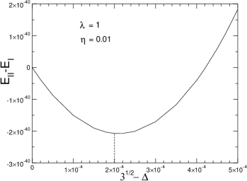
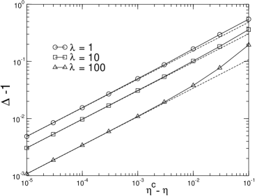
interestingly does not depend in the leading order on $\lambda$. It corresponds to the minimum of energy $E_{\rm II}(\epsilon)$ as ${\partial^{2}_{\epsilon}}E_{\rm II}(\sqrt{3}-\epsilon,\eta,\lambda)|_{\epsilon=\epsilon^{*}}=2f_{2}(\eta,\lambda)>0$. For $\lambda=1$ and $\eta=0.01$, we checked the result (23) numerically in Fig. 3. One can see that $E_{\rm II}(\epsilon)$, calculated using the complete formula (16) truncated at $M=5$ has a minimum rather close to the value $\epsilon^{*}=0.0002$ predicted by our asymptotic formula (20).

Figure 3: $E_{\rm II}(\Delta,\eta)-E_{\rm I}(\eta)$ as a function of $\sqrt{3}-\Delta$ for the fixed values of $\lambda=1$ and $\eta=0.01$. The value of $\epsilon^{*}=0.0002$, which provides the energy minimum according to the asymptotic formula (23) is depicted by the vertical dashed line for comparison. Note that the energy differences are extremely small.

We conclude that phase I is stable only at $\eta=0$ and for an arbitrarily small positive $\eta$ we enter the region of phase II. It is interesting that the asymptotic $\eta\to 0$ predictions for the unscreened Coulomb $\lambda=0$ case (21) and for $\lambda>0$ (23) exhibit the same $\eta^{2}$ dependence, but there is a skip in the prefactors from $7.14064\ldots$ at $\lambda=0$ to $2$ for $\lambda>0$. The fact that in the previous works Goldoni ; Weis ; Messina phase I was detected also for small positive values of $\eta$ is probably related to extremely small deviation of $\sqrt{3}-\Delta^{*}\propto\eta^{2}$ which are “invisible” by standard numerical methods.

IV Second-order transition between phases II and III

Let us parametrize $\Delta=\exp({\epsilon})$. The symmetry $\Delta\to 1/\Delta$ of the energy (16) is then equivalent to the transformation $\epsilon\to-\epsilon$ and the energy is an even function of $\epsilon$. The Ginsburg-Landau form of its expansion around $\epsilon=0$ reads as

$$E_{\rm II}({\rm e}^{\epsilon},\eta,\lambda)=E_{\rm III}(\eta,\lambda)+g_{2}(\eta,\lambda)\epsilon^{2}+g_{4}(\eta,\lambda)\epsilon^{4}+\ldots$$ (24)

The explicit expression for $g_{2}$ is given in Appendix C and a rather cumbersome expression for $g_{4}$ is also at our disposal. The critical point is given by the vanishing of the prefactor

$$g_{2}(\eta^{c},\lambda^{c})=0.$$ (25)

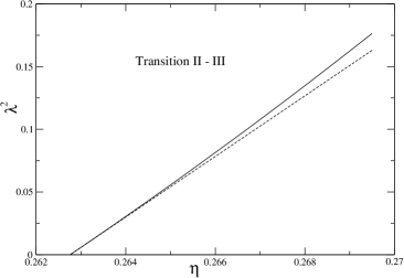
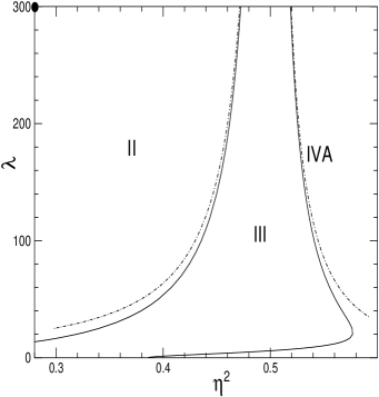
We used this equation to get the (dashed) critical line between phases II and III in Fig. 4. Our definition of $\eta$ differs from that of the dimensionless distance in the paper of Messina and Löwen Messina , namely $\eta^{2}=\eta_{\rm ML}$. To maintain the full comparability, we shall present the phase diagram using the variable $\eta^{2}$.

Figure 4: Phase diagram of the Yukawa bilayer. Dashed lines denote the second-order phase transitions, solid lines correspond to the first-order phase transitions. The important data for the hard-sphere limit $\lambda\to\infty$ are added on the top.

IV.1 Critical behavior

To obtain the critical behavior, we note that the functions $g_{2}$ and $g_{4}$ in Eq. (24) behave in the vicinity of the critical point $(\eta^{c},\lambda^{c})$ as follows

$$g_{2}(\eta,\lambda) = g_{21}(\lambda^{c})(\eta^{c}-\eta)+{\cal O}[(\eta^{c}-\eta)^{2}],$$

$$g_{4}(\eta,\lambda) = g_{40}(\lambda^{c})+{\cal O}(\eta^{c}-\eta),$$ (26)

where $g_{21}(\lambda^{c})<0$ and $g_{40}(\lambda^{c})>0$ for all $\lambda^{c}$. The minimum energy is reached at $\epsilon^{*}\approx\Delta^{*}-1$ given by

$$\frac{\partial}{\partial\epsilon}E_{\rm II}({\rm e}^{\epsilon},\eta,\lambda)\big{|}_{\epsilon=\epsilon^{*}}\approx 2g_{2}(\eta,\lambda)\epsilon^{*}+4g_{4}(\eta,\lambda)(\epsilon^{*})^{3}=0.$$ (27)

For $\eta>\eta^{c}$, there is only one solution $\epsilon^{*}=0$ which corresponds to the square lattice of phase III. For $\eta<\eta^{c}$, we get one trivial (unphysical) solution $\epsilon^{*}=0$ and two non-trivial conjugate solutions $\pm\epsilon^{*}$ with

$$\epsilon^{*}=\left(-\frac{g_{2}(\eta,\lambda)}{2g_{4}(\eta,\lambda)}\right)^{1/2}\approx\left(-\frac{g_{21}(\lambda^{c})}{2g_{40}(\lambda^{c})}\right)^{1/2}\sqrt{\eta^{c}-\eta},$$ (28)

$\eta\to(\eta^{c})^{-}$. The order parameter $\epsilon^{*}\propto\sqrt{\eta^{c}-\eta}$ is thus associated with the mean-field critical index $\beta_{\rm MF}=1/2$ for every $\lambda\geq 0$. The dependence of $\Delta-1$ on $\eta^{c}-\eta$ is shown in Fig. 5 for three values of $\lambda=1,10,100$. Near the critical point ($\eta^{c}-\eta$ small), the asymptotic relation (28) (dashed lines) fits perfectly the numerical data from minimization of the energy $E_{\rm II}$ (12) (full lines). In the logarithmic plot, for all values of $\lambda$ the slope of $\Delta-1$ vs. $\eta^{c}-\eta$ is very close to 0.5 in the region of small and intermediate values of $\eta^{c}-\eta$, confirming the value $1/2$ of the mean-field critical index $\beta_{\rm MF}$ for all values of $\lambda$.

Figure 5: Order parameter close to the critical point of the transition II-III for three values of $\lambda=1,10,100$. Full lines follow from numerical minimization of the energy (16). The slope of lines is close to $\beta_{\rm MF}=1/2$. Dashed lines represent the asymptotic $\eta\to(\eta^{c})^{-}$ relation (28).

From Eq. (24), the energy difference of phases II and III close to the critical point is given by

$$E_{\rm II}({\rm e}^{\epsilon},\eta,\lambda)-E_{\rm III}(\eta,\lambda)\sim-\frac{g_{21}^{2}(\lambda^{c})}{4g_{40}(\lambda^{c})}(\eta^{c}-\eta)^{2}.$$ (29)

The critical singularity should be of type $(\eta^{c}-\eta)^{2-\alpha}$ implying the mean-field critical index $\alpha_{\rm MF}=0$ for any $\lambda$.

To obtain another two critical indices, we add to the energy (24) the symmetry-breaking term $-h\epsilon$, where a small positive external field $h\to 0^{+}$ is linearly coupled to the order parameter. The optimization condition for the energy with respect to $\epsilon$ now takes the form

$$2g_{2}(\eta,\lambda)\epsilon^{*}+4g_{4}(\eta,\lambda)(\epsilon^{*})^{3}-h=0.$$ (30)

At the critical point, since $g_{2}(\eta^{c},\lambda^{c})=0$ and $g_{4}(\eta^{c},\lambda^{c})=g_{40}(\lambda^{c})$, we find from (30) that

$$\epsilon^{*}=\left[\frac{h}{4g_{40}(\lambda^{c})}\right]^{1/3}.$$ (31)

This critical singularity should be of type $h^{1/\delta}$, which leads to the mean-field critical index $\delta_{\rm MF}=3$ for any $\lambda$. Performing the derivative of Eq. (30) with respect to $h$, we find for the field succeptibility close to the critical point:

$$\frac{\partial\epsilon^{*}}{\partial h}\Bigg{|}_{h=0}=\frac{1}{-4g_{21}(\lambda^{c})}\frac{1}{\eta^{c}-\eta},\qquad\eta\to(\eta^{c})^{-}.$$ (32)

The corresponding critical singularity $(\eta-\eta^{c})^{-\gamma}$ leads to the mean-field critical index $\gamma_{\rm MF}=1$ for arbitrary $\lambda$.

It is easy to verify that our mean-field critical indices

$$\alpha_{\rm MF}=0,\quad\beta_{\rm MF}=\frac{1}{2},\quad\gamma_{\rm MF}=1,\quad\delta_{\rm MF}=3$$ (33)

fulfill two standard scaling relations Ma

$$2-\alpha=2\beta+\gamma=\beta(\delta+1).$$ (34)

Since there are no fluctuations in our system at zero temperature, the critical indices $\eta$ and $\nu$, related to the particle correlation function, are not defined.

IV.2 Coulomb $\lambda\to 0$ limit of the critical line

We reproduce $\eta^{c}(0)=0.2627602682$ Samaj1 in the Coulomb $\lambda\to 0$ limit. It is shown in Appendix C that the asymptotic $\lambda\to 0$ shape of the critical line between phases II and III is parabolic:

$$\lambda^{2}\approx c_{23}[\eta^{c}-\eta^{c}(0)],\qquad c_{23}\approx 24.173744.$$ (35)

This formula is compared to the critical line evaluated numerically by using the relation (25) in Fig. 6.

Figure 6: The critical line between phases II and III near the unscreened Coulomb $\lambda\to 0$ limit. Full line follows from the numerical evaluation by using the relation $g_{2}(\eta,\lambda)=0$. Dashed line corresponds to the asymptotic formula (35).

IV.3 Hard-spheres $\lambda\to\infty$ limit of the critical line

In the hard-spheres limit $\lambda\to\infty$, the critical point for the ${\rm II}\to{\rm III}$ transition is $(\eta^{c})^{2}\to 1/2$ Messina . The convergence to this value is extraordinarily slow. Let us analyze this limit in the critical equation $g_{2}(\eta,\lambda)=0$. Applying the asymptotic formulas for the generalized Misra functions (73) and (74) to $g_{2}(\eta,\lambda)$ given by the series (79), most summands become exponentially small compared to the few leading terms proportional to $\exp(-\lambda/\eta)$. In particular, we can neglect completely the first four sums in Eq. (79) since all terms behave as $\exp(-c\lambda^{2})$ and the sixth sum because we get at least $\exp(-\sqrt{2}\lambda/\eta)$ for the $j=k=1$ term. Those leading terms appear in the fifth sum with $j=1$ and the seventh sum with $j=k=1$. The ones with e. g. $j=2$, $k=1$ etc. are exponentially small again compared to the leading ones. In the last sum the $z_{7/2}(.,.)$ term has zero prefactor for $j=k$. We are left with the three-terms expression

$$g_{2}(\eta,\lambda) \approx z_{7/2}\left(\frac{\lambda^{2}}{4\eta^{2}},1\right)-z_{5/2}\left(\frac{\lambda^{2}}{4\eta^{2}},1\right)$$ (36)

$$-\frac{1}{2}z_{5/2}\left(\frac{\lambda^{2}}{4\eta^{2}},\eta^{2}+\frac{1}{2}\right),\qquad\lambda\gg 1.$$

Applying the asymptotic formula (74), we rewrite the rhs of this expression as

$$\frac{\sqrt{\pi}\lambda{\rm e}^{-\frac{\lambda}{\eta}}}{4\eta}\left[\frac{\lambda}{\eta}+1+\frac{\eta}{\lambda}-\frac{1+\frac{\eta}{\lambda\sqrt{\eta^{2}+\frac{1}{2}}}}{\eta^{2}+\frac{1}{2}}{\rm e}^{\frac{\lambda}{\eta}\left(1-\sqrt{\eta^{2}+\frac{1}{2}}\right)}\right].$$ (37)

The critical condition $g_{2}(\eta,\lambda)=0$ implies a transcendental formula for $\eta(\lambda)$:

$$\frac{\left(\frac{\lambda}{\eta}+1+\frac{\eta}{\lambda}\right)\left(\eta^{2}+\frac{1}{2}\right)}{1+\frac{\eta}{\lambda\sqrt{\eta^{2}+\frac{1}{2}}}}={\rm e}^{\frac{\lambda}{\eta}\left(1-\sqrt{\eta^{2}+\frac{1}{2}}\right)}.$$ (38)

The exponential term can equal to the rational one only if $1-\sqrt{\eta^{2}+1/2}$ is close to zero, i. e. $\eta^{2}\to 1/2$ in the $\lambda\to\infty$ limit as expected. The next terms of the large-$\lambda$ expansion of $\eta(\lambda)$ can be derived straightforwardly, with the result

$$\eta\approx\frac{1}{\sqrt{2}}-\frac{\ln{\lambda}}{\lambda}-\frac{\ln{2}}{2\lambda}+{\cal O}\left(\frac{\ln^{2}{\lambda}}{\lambda^{2}}\right).$$ (39)

In general, the series contains the terms of the form $(\ln\lambda)^{m}/\lambda^{n}$ where $m$, $n$ are integers such that $0\leq m\leq n$. The first correction of type $(\ln\lambda)/\lambda$ explains a slow convergence of the results as $\lambda\to\infty$.

Figure 7: An excerption of the phase diagram for Yukawa particles for the second-order phase transitions ${\rm II}\to{\rm III}$ and ${\rm III}\to{\rm IVA}$. The solid lines denote the critical lines obtained numerically by using Eq. (25) and (42), respectively. The dash-dotted lines correspond to the asymptotic large-$\lambda$ formulas (39) and (47).

The asymptotic formula (39), taken for $\eta^{2}$, is plotted in Fig. 7 by the dash-dotted line. We see that it reproduces adequately the numerical results for the critical line (solid line) in a large region of the phase diagram. It can be shown that the next term of the series (39) reads as $3\ln^{2}\lambda/(2^{3/2}\lambda^{2})$; plotting the asymptotic formula (39) with this term included makes the difference with the numerical solid line invisible by eye.

V Energy for structures IVA, IVB and V

It was already mentioned that structures IVA, V and even III are special cases of the most general phase IVB. Hence we will sketch the derivation of the energy per particle for the latter. The elementary cell is a rhombus with the angle $\phi$ between the vectors ${\bm{a}_{1}}$ and ${\bm{a}_{2}}$ of the same magnitude $a$, see Fig. 2. The density of particles on one plate is $\sigma=1/(a^{2}\sin\phi)$. We will prefer the parametrization of the angle by $\delta=\tan(\phi/2)$. Another free parameter is $\alpha\in[1/3,1/2]$ measuring the diagonal shift ${\bm{c}}$ of the lattice on the opposite layer, see formula(2). The square of the lattice vector can be written as $|{\bm{r}}_{jk}|^{2}=a^{2}[(j+k)^{2}\cos^{2}(\phi/2)+(j-k)^{2}\sin^{2}(\phi/2)]$. Next we distinguish the cases when $j+k$ is an even or odd integer and go to the summation over new indices $m$ and $n$; details of this technicality and of the next steps can be found in Sec. III of paper Samaj1 . The main difference is that we get $(n+\alpha)^{2}$ and $(n-1/2+\alpha)^{2}$ instead of $n^{2}$ and $(n-1/2)^{2}$ for the interlayer contribution. Applying the Poisson formula (11) creates additional factors $\exp(2\pi in\alpha)$ and $\exp[2\pi in(\alpha-1/2)]$. Reducing the summation over $\{-\infty,\infty\}$ to $\{1,\infty\}$ turns these factors to $2\cos(2\pi n\alpha)$ and $2\cos[2\pi n(\alpha-1/2)]$, respectively. The final formula for the energy per particle of phase IVB reads

$$E_{\rm IVB} = \frac{\eta}{2\sqrt{2\pi}\lambda}\Bigg{(}2\sum_{j=1}^{\infty}\left[z_{3/2}\left(0,\frac{\lambda^{2}}{2\pi^{2}\eta^{2}}+j^{2}\delta\right)+z_{3/2}\left(0,\frac{\lambda^{2}}{2\pi^{2}\eta^{2}}+j^{2}/\delta\right)\right]\bigg{[}1+(-1)^{j}\bigg{]}$$ (40)

$$+4\sum_{j,k=1}^{\infty}\left[1+(-1)^{j+k}\right]z_{3/2}\left(0,\frac{\lambda^{2}}{2\pi^{2}\eta^{2}}+j^{2}/\delta+k^{2}\delta\right)-\pi z_{1/2}\left(0,\frac{\lambda^{2}}{2\eta^{2}\pi^{2}}\right)$$

$$+2\sum_{j=1}^{\infty}\left[\cos(2\pi j\alpha)z_{3/2}\left(\pi^{2}\eta^{2}/2,\frac{\lambda^{2}}{2\pi^{2}\eta^{2}}+j^{2}\delta\right)+z_{3/2}\left(\pi^{2}\eta^{2}/2,\frac{\lambda^{2}}{2\pi^{2}\eta^{2}}+j^{2}/\delta\right)\right]$$

$$+2\sum_{j=1}^{\infty}\left\{\cos\left[2\pi j\left(\alpha-\frac{1}{2}\right)\right]z_{3/2}\left(\pi^{2}\eta^{2}/2,\frac{\lambda^{2}}{2\pi^{2}\eta^{2}}+j^{2}\delta\right)+(-1)^{j}z_{3/2}\left(\pi^{2}\eta^{2}/2,\frac{\lambda^{2}}{2\pi^{2}\eta^{2}}+j^{2}/\delta\right)\right\}$$

$$+4\sum_{j,k=1}^{\infty}\left\{\cos(2\pi j\alpha)+\cos\left[2\pi j\left(\alpha-\frac{1}{2}\right)\right](-1)^{k}\right\}z_{3/2}\left(\pi^{2}\eta^{2}/2,\frac{\lambda^{2}}{2\pi^{2}\eta^{2}}+j^{2}\delta+k^{2}/\delta\right)$$

$$+2\sum_{j=1}^{\infty}\left[z_{3/2}\left(\frac{\lambda^{2}}{2\eta^{2}},j^{2}\delta\right)+z_{3/2}\left(\frac{\lambda^{2}}{2\eta^{2}},j^{2}/\delta\right)\right]+4\sum_{j,k=1}^{\infty}z_{3/2}\left(\frac{\lambda^{2}}{2\eta^{2}},j^{2}/\delta+k^{2}\delta\right)-2\pi z_{1/2}\left(\frac{\lambda^{2}}{2\eta^{2}},0\right)$$

$$+\sum_{j,k=-\infty}^{\infty}\left\{z_{3/2}\left[\frac{\lambda^{2}}{2\eta^{2}},\eta^{2}/2+\frac{1}{\delta}(j+\alpha)^{2}+k^{2}\delta\right]+z_{3/2}\left[\frac{\lambda^{2}}{2\eta^{2}},\eta^{2}/2+\frac{1}{\delta}(j+\alpha-1/2)^{2}+(k-1/2)^{2}\delta\right]\right\}$$

$$-2\pi z_{1/2}\left(\frac{\lambda^{2}}{2\eta^{2}},\eta^{2}/2\right)+4\sum_{j,k=1}^{\infty}z_{3/2}\left[\frac{\lambda^{2}}{2\eta^{2}},\frac{1}{\delta}\left(j-\frac{1}{2}\right)^{2}+\left(k-\frac{1}{2}\right)^{2}\delta\right]\Bigg{)}+\pi\frac{\eta^{2}}{\lambda^{2}}\left(1+{\rm e}^{-\lambda}\right).$$

VI Transition between phases III and IVA

One can verify that for the structure IVA with $\alpha=1/2$ the energy (40) possesses the symmetry $\delta\to 1/\delta$. The case $\delta=1$ or $\phi=\pi/2$ is the fixed point of the transformation $\delta\to 1/\delta$ and corresponds to the critical point between phases III and IVA. In full analogy with the transition between phases II and III, we parametrize $\delta=\exp(-\epsilon)$ so that the energy of phase IVA becomes an even function of $\epsilon$. The expansion of the energy (40) around the critical point $\delta=1$ in powers of small $\epsilon$ takes the form

$$E_{\rm IVA}({\rm e}^{-\epsilon},\eta,\lambda) = E_{\rm III}(1,\eta,\lambda)+h_{2}(\eta,\lambda)\epsilon^{2}$$ (41)

$$+h_{4}(\eta,\lambda)\epsilon^{4}+\ldots.$$

The explicit formula for $h_{2}$ in terms of the generalized Misra functions is presented in Appendix D and $h_{4}$ is also at our disposal. The critical line between phases III and IVA is once again given by vanishing of the prefactor

$$h_{2}(\eta^{c},\lambda^{c})=0,$$ (42)

see Figs. 4 and 7.

VI.1 Critical behavior

The expansion of the coefficients $h_{2}$ and $h_{4}$ around the critical point $(\eta^{c},\lambda^{c})$ is analogous to the previous case of the second-order transition between phases II and III. The leading terms are $h_{2}(\eta,\lambda)\approx h_{21}(\lambda^{c})(\eta-\eta^{c})$ and $h_{4}(\eta,\lambda)\approx h_{40}(\lambda^{c})$, where $h_{21}(\lambda^{c})<0$ and $h_{40}(\lambda^{c})>0$ for all $\lambda_{c}$. Optimizing the energy $E_{\rm IVA}$ with respect to $\epsilon$, the stationary solution $\epsilon^{*}=1-\delta^{*}$ behaves as

$$\epsilon^{*}=\left(-\frac{h_{2}(\eta,\lambda)}{2h_{4}(\eta,\lambda)}\right)^{1/2}\approx\left(-\frac{h_{21}(\lambda^{c})}{2h_{40}(\lambda^{c})}\right)^{1/2}\sqrt{\eta-\eta^{c}}$$ (43)

with $\eta\to(\eta^{c})^{+}$. The order parameter $\epsilon^{*}$ has again the singular behavior of mean-field type with critical index $\beta_{\rm MF}=1/2$. We tested this results numerically in a plot analogous to Fig. 5 and got the slope $\beta\approx 0.499$. Without going into details, also other critical indices attain their mean-field values (33).

VI.2 Coulomb $\lambda\to 0$ limit of the critical line

The week screening (small $\lambda$) case of the phase transitions III-IVA and IVA-V was studied by Monte Carlo methods in Ref. Mazars08 .

We reproduce $\eta^{c}(0)=0.6214809246$ Samaj1 in the Coulomb $\lambda\to 0$ limit. The asymptotic shape of the critical line for small $\lambda$ is again parabolic, see Appendix D:

$$\lambda^{2}\approx c_{34}[\eta^{c}-\eta^{c}(0)],\qquad c_{34}\approx 149.7837254.$$ (44)

This asymptotic result is compared with the numerical calculation of the critical line directly from the relation (42) in Fig. 8.

Figure 8: Transition III-IVA near the Coulomb $\lambda\to 0$ limit. The full line follows from the numerical treatment of the relation $h_{2}(\eta,\lambda)=0$. The dashed line corresponds to the asymptotic formula (44).

VI.3 Hard-spheres $\lambda\to\infty$ limit of the critical line

In the hard-spheres limit $\lambda\to\infty$, the critical point for the ${\rm III}\to{\rm IVA}$ transition is $(\eta^{c})^{2}\to 1/2$ Messina , the same as in the previous case of the ${\rm II}\to{\rm III}$ transition. Let us analyze the large-$\lambda$ limit of the critical relation $h_{2}(\eta,\lambda)=0$. In the same way as for $g_{2}$, we get three leading terms from the seventh and ninth (last) sums of Eq. (84):

$$\frac{1}{16}z_{7/2}\left(\frac{\lambda^{2}}{2\eta^{2}},\frac{\eta^{2}}{2}+\frac{1}{4}\right)-\frac{1}{4}z_{5/2}\left(\frac{\lambda^{2}}{2\eta^{2}},\frac{\eta^{2}}{2}+\frac{1}{4}\right)$$

$$-\frac{1}{2}z_{5/2}\left(\frac{\lambda^{2}}{2\eta^{2}},\frac{1}{2}\right)=0,\qquad\lambda\gg 1.$$ (45)

The application of the asymptotic relations (74) to this equation implies

$$\sqrt{\frac{\pi}{2}}\frac{\lambda}{\eta}{\rm e}^{-\frac{\lambda}{\eta}}\Bigg{\{}\Bigg{[}\frac{\lambda}{8\eta\left(\eta^{2}+\frac{1}{2}\right)^{3/2}}\Bigg{(}1+\frac{3\eta}{\lambda\sqrt{\eta^{2}+\frac{1}{2}}}$$

$$+\frac{3\eta^{2}}{\lambda^{2}(\eta^{2}+\frac{1}{2})}\Bigg{)}-\frac{1}{2(\eta^{2}+\frac{1}{2})}\left(1+\frac{\eta}{\lambda\sqrt{\eta^{2}+\frac{1}{2}}}\right)\Bigg{]}$$

$$\times{\rm e}^{\frac{\lambda}{\eta}\left(1-\sqrt{\eta^{2}+1/2}\right)}-\left(1+\frac{\eta}{\lambda}\right)\Bigg{\}}=0.$$ (46)

The root of the expression in the largest parentheses yields

$$\eta \approx \frac{1}{\sqrt{2}}+\frac{\ln\lambda}{\lambda}+-\frac{5\ln 2}{2\lambda}$$ (47)

$$+\frac{3}{4}\sqrt{2}\left(\frac{\ln{\lambda}}{\lambda}\right)^{2}+{\cal O}\left(\frac{\ln{\lambda}}{\lambda^{2}}\right).$$

This asymptotic formula, taken for $\eta^{2}$, is plotted in Fig. 7 by the dash-dotted line. The comparison with the numerical results for the critical line (solid line) is very good.

VII Phase transitions IVA - V, IVA - IVB and IVB - V

All phase transitions IVA - V, IVA - IVB and IVB - V are of first order due to a discontinuous change of both structure parameters $\delta$ and $\alpha$. For phase IVB one has to minimize numerically the energy (40) with respect to two parameters $\delta$ and $\alpha$, which is tedious but feasible.

We found that for $\lambda<27.4436$ phase IVA goes over directly to phase V without entering the intermediate phase IVB. On the transition line, the parameter $\alpha$ jumps from 1/2 to 1/3. In the Coulomb limit $\lambda\to 0$ we get $\eta^{t}(0)=0.732416$, $\delta^{t}=0.69334$ for phase IVA Samaj1 whereas for the rigid phase V $\delta^{t}=\tan(\pi/6)=1/\sqrt{3}\approx 0.57735$. The shape of the transition line is again parabolic, we can approximate it empirically by

$$\lambda^{2}\approx c_{4A5}[\eta^{t}(0)-\eta^{t}],\qquad c_{4A5}\approx 805.3,$$ (48)

but now the parabola is reversed giving rise to the multiple reentrant behavior, see Figs. 4 and 9.

Figure 9: A detailed view of the phase diagram around the tricritical point. The sector of phase IVA is connected by a narrow channel.

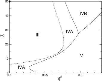
The non-trivial $\delta^{t}$ for phase IVA increases to approximately 0.926 at $\lambda=14$ and then slightly decreases to 0.853081 at $\lambda=27.4436$. In Ref. Messina it was anticipated that there exist two disjunct regions of phase IVA in the phase diagram. Our more precise calculations indicate that there exists a narrow connecting channel merging these two regions into one, see Fig. 9. The maximum value of $\delta^{t}$ for phase IVA is achieved when the channel is the most narrow so that it does not decrease too much from the value $\delta=1$ for phase III. Looking at Figs. 4 and 9 we can confirm the double reentrant scenario IVA-V-IVA-III-IVA-IVB Messina , restricted to a more precise interval $0.5275<\eta^{2}<0.53643$.

For $\lambda>27.4436$, the phase IVB takes place and we have first-order transitions IVA-IVB and IVB-V, see Figs. 4 and 9.

As concerns the transition line IVA - IVB, for $\lambda\to\infty$ it should asymptotically approach the value $(\eta^{t})^{2}\to 1/2$ so that phase IVA is absent in the hard-spheres limit Messina . The value of $\delta^{t}$ in phase IVA increases from 0.85308 at $\lambda=27.4436$ towards 1 for very large $\lambda$. Concerning phase IVB, $\delta^{t}$ increases from 0.763284 at $\lambda=27.4436$ to 1 for very large $\lambda$ and the other parameter $\alpha^{t}$ from 0.41358 to 0.5 along the same transition line. Thus, in the hard-spheres limit, the values $\delta^{t}\to 1$ and $\alpha^{t}\to 1/2$ of phase III (see the top of Fig. 4) will be attained as expected.

Still in the hard-spheres limit $\lambda\to\infty$, the transition line IVB-V should reach the point $\eta^{t}\approx 0.877\ldots$ Messina . Numerically, we got mere $\eta^{t}=0.864133\ldots$ even for $\lambda=500$. The convergence is rather slow again, we have $\delta^{t}=0.58102$ and $\alpha^{t}=0.334428$ for phase IVB at the same $\lambda=500$ value, gradually approaching the values 0.57735 and 1/3 of phase V, respectively, with ${\cal O}(1/\lambda)$ corrections of both structure parameters. Now we want to derive the above hard-spheres result from our formalism. We recall that the energy $E_{\rm IVB}$ is given by Eq. (40) and $E_{\rm V}$ is its special case for $\delta=1/\sqrt{3}$ and $\alpha=1/3$. We apply the asymptotic formulas (73) and (74) to the $\lambda\to\infty$ limit of Eq. (40) and neglect exponentially small terms. Five summands remain dominant; one from the sixth sum with $j=1$, three from the eighths (last but one) sum, namely both terms with $j=k=0$ and the second one with $j=0$, $k=1$ plus the $j=k=0$ term from the ninth (last) sum:

$$E_{\rm IVB} \approx \frac{\eta}{2\sqrt{2\pi}\lambda}\biggl{\{}2z_{3/2}\left(\frac{\lambda^{2}}{2\eta^{2}},\delta\right)$$ (49)

$$+z_{3/2}\left(\frac{\lambda^{2}}{2\eta^{2}},\frac{\eta^{2}}{2}+\frac{\alpha^{2}}{\delta}\right)$$

$$+2\ z_{3/2}\left[\frac{\lambda^{2}}{2\eta^{2}},\frac{\eta^{2}}{2}+\frac{(\alpha-1/2)^{2}}{\delta}+\frac{\delta}{4}\right]$$

$$+4\ z_{3/2}\left(\frac{\lambda^{2}}{2\eta^{2}},\frac{1}{4\delta}+\frac{\delta}{4}\right)\biggr{\}}.$$

Notice that two identical terms merged to the one on the third line. All these summands should be of the same order for very large $\lambda$. Since the asymptotic relations (74) imply that $z_{\nu}(x,y)\propto\exp(-2\sqrt{xy})$ for $x\to\infty$, and the first argument $x=\lambda^{2}/(2\eta^{2})$ is common for the summands, the second arguments must coincide as well. Thus we have

$$\delta=\frac{\eta^{2}}{2}+\frac{\alpha^{2}}{\delta}=\frac{\eta^{2}}{2}+\frac{(\alpha-\frac{1}{2})^{2}}{\delta}+\frac{\delta}{4}=\frac{1}{4\delta}+\frac{\delta}{4}.$$ (50)

This equalities yield the expected asymptotic values of the structure parameters $\delta=1/\sqrt{3}$ and $\alpha=1/3$. Simultaneously,

$$\eta^{t}=\frac{2}{3^{3/4}}\approx 0.877383\ldots,\qquad\lambda\to\infty.$$ (51)

This value can be rederived from purely geometric considerations, too. We have already mentioned that the particle density at one plate in phase V is $\sigma=1/[a^{2}\sin(\pi/3)]=2/(a^{2}\sqrt{3})$. For dense packed hard spheres of radius $a$, the perpendicular distance of two layers of triangular lattices is $d=\sqrt{2/3}\ a$, see e.g. Schmidt . Inserting these values into $\eta=d\sqrt{\sigma}$ yields immediately (51).

We confirm that in the hard-spheres limit the transition IVB-V will undergo no stepwise changes of structure parameters and it will be of the second order, as expected.

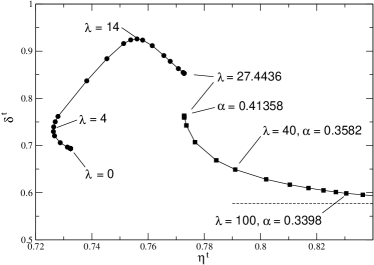
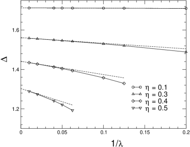
In Fig. 10, we present the transition values of the structure parameters $\delta^{t}$ and $\alpha^{t}$ for phases IVA and IVB at first-order transitions IVA - V (left, $\lambda\in[0,27.4436]$) and IVB - V (right, $\lambda\in[27.4436,\infty]$). The left and right line fragments are separated by a gap, illustrating the step-wise change of structure parameters when going from phase IVA to IVB. We recall that the parameters of phase V are always fixed to $\delta^{t}=1/\sqrt{3}$ and $\alpha^{t}=1/3$. We found a tricritical point at $\eta^{c}=0.772814$ and $\lambda^{c}=27.4436$ where the three phases IVA, IVB and V coexist.

Figure 10: The transition parameters $\delta^{t}$ and $\eta^{t}$ along the phase transition lines IVA-V (left) and IVB-V (right). Along two line fragments, $\lambda$ increases from 0 to $\infty$. For the left fragment, the parameter $\alpha=1/2$ for phase IVA and $\alpha=1/3$ for phase V. There is a discontinuity in the parameters $\delta$ and $\alpha$ between phases IVA and IVB at the tricritical point with $\lambda=27.4436$. The values of $\alpha$ on the right fragment correspond to phase IVB. In the hard-spheres limit $\lambda\to\infty$, the line ends up at the critical point $(\eta^{c}=0.877383,\delta^{c}=1/\sqrt{3})$.

VIII The energy plot

We want to compare the values of the optimized energy per particle for various values of $\lambda$ and $\eta$. We plot $E(\eta)$ for several fixed values of $\lambda$ in Fig. 11. These energies vary by orders of magnitude, thus we have chosen semilogarithmic scale.

First we consider two limiting cases. For $\eta\ll 1$ and $\lambda>0$, according to (18) and (22) the energy of the corresponding phase II $\ln(E_{\rm II})\approx-3^{1/4}\lambda/\eta$ and so $\ln{E}$ diverges if $\eta\to 0$. More interesting is the optimal energy of phase V, $E_{\rm V}$, for $\eta\gg 1$. We were used to get the Coulomb limit as $\lambda\to 0$, but we can obtain this limit also for medium $\lambda$ and very large $\eta$, as the ratio $\lambda/\eta\to 0$ again. For $\eta\gg\lambda$, using the asymptotic formulas for the generalized Misra functions (Appendix A) we obtain from (40) that

$$E_{\rm V}=\pi\frac{\eta^{2}}{\lambda^{2}}\left(1+{\rm e}^{-\lambda}\right)+c_{M}\frac{\eta}{\lambda}+{\cal O}(1),$$ (52)

where $c_{M}=-1.9605158...$ is the Madelung constant of the Coulomb potential for the hexagonal lattice; for an explicit representation of the Madelung constant in terms of $z_{\nu}(0,y)$ functions, see Eq. (24) with $\Delta=\sqrt{3}$ and $\eta=0$ of Ref. Samaj1 . The leading term is the (minus) background energy (13).

Figure 11: The dependence of the energy per Yukawa particle $E$ on the dimensionless distance $\eta$ for four values of $\lambda=1,10,20,35$, in semilogarithmic scale.

Figure 12: The derivative $\partial E/\partial\eta$ for $\lambda=20$. Full circle corresponds to the second-order transition III-IVA, dashed line marks the discontinuity at the first-order transition IVA-V.

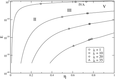
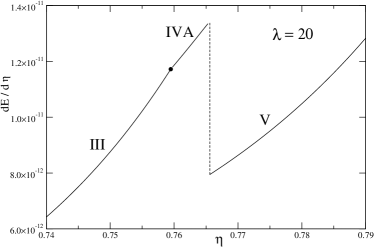
We see in Fig. 11 for few fixed values of $\lambda$ that the energy is a monotonously increasing function of the dimensionless distance $\eta$. This means that the force between the plates is always attractive. The non-analyticities at transition points are not clearly manifested in this scale. Therefore, for $\lambda=20$, we performed the derivative $\partial E/\partial\eta$, directly for rigid structures and numerically using $E_{\rm IVA}$ minimized with respect to $\delta$ for phase IVA. The obtained results are plotted in Fig. 12. We see the expected continuous but non-analytic behavior at the second-order transition point III-IVA as well as a jump discontinuity at the first order transition IVA-V.

IX Internal parameters of the phases near hard-spheres limit

In and close to the limit of hard spheres $\lambda\to\infty$, the expressions for the energies of the structures in terms of the generalized Misra functions admit an asymptotic analysis. This fact permits us to determine the $\eta$-dependence of the structure parameters of the present soft phases II and IVB in the $\lambda\to\infty$ limit and eventually to derive their leading correction for large but finite $\lambda$.

IX.1 Aspect ratio $\Delta$ of phase II at and near hard spheres

The dependence of the aspect ratio $\Delta_{\rm HS}$ on $\eta$ for phase II is well known in the hard-spheres limit $\lambda\to\infty$ Messina :

$$\Delta_{\rm HS}(\eta)=\sqrt{4\eta^{4}+3}-2\eta^{2}.$$ (53)

In the following, we derive this result and the first $1/\lambda$ correction to it by using our method.

For $\lambda\gg 1$, most of terms in the energy of phase II (16) become exponentially small (we exclude from the discussion trivial terms which do not depend on $\Delta$); only the term $j=1$ in the sixth sum and the term $j=k=1$ in the eighth (last) sum contribute. As soon as $\Delta>1$, using (74) we get

$$E_{\rm II}\approx\frac{\eta}{\sqrt{\pi}\lambda}\left[z_{\frac{3}{2}}\left(\frac{\lambda^{2}}{4\eta^{2}},\frac{1}{\Delta}\right)+2z_{\frac{3}{2}}\left(\frac{\lambda^{2}}{4\eta^{2}},\eta^{2}+\frac{\Delta}{4}+\frac{1}{4\Delta}\right)\right]$$

$$\approx\frac{\eta}{\lambda}\left(\sqrt{\Delta}{\rm e}^{-\frac{\lambda}{\eta\sqrt{\Delta}}}+\frac{2}{\sqrt{\eta^{2}+\frac{\Delta}{4}+\frac{1}{4\Delta}}}{\rm e}^{-\frac{\lambda}{\eta}\sqrt{\eta^{2}+\frac{\Delta}{4}+\frac{1}{4\Delta}}}\right).$$

(54)

The minimum of the energy is given by $\partial E_{\rm II}/\partial\Delta=0$, which implies

$$\left(\frac{1}{2\sqrt{\Delta}}+\frac{\lambda}{2\Delta\eta}\right){\rm e}^{-\frac{\lambda}{\eta\sqrt{\Delta}}}=\frac{1-\frac{1}{\Delta^{2}}}{4\eta^{2}+\Delta+\frac{1}{\Delta}}$$

$$\times\left(\frac{1}{\sqrt{\eta^{2}+\frac{\Delta}{4}+\frac{1}{4\Delta}}}+\frac{\lambda}{\eta}\right){\rm e}^{-\frac{\lambda}{\eta}\sqrt{\eta^{2}+\frac{\Delta}{4}+\frac{1}{4\Delta}}}.$$ (55)

If we want to reproduce just the hard-spheres limit $\lambda\to\infty$, we can say that exponentials are by far more significant than rationals and their arguments must become the same, i.e. $\sqrt{\eta^{2}+\Delta/4+1/(4\Delta)}=1/\sqrt{\Delta}$ which leads to the known result (53). Numerics suggests that the correction is of the type $1/\lambda$, i. e.

$$\Delta\approx\Delta_{\rm HS}+\frac{a(\eta)}{\lambda}=\sqrt{4\eta^{4}+3}-2\eta^{2}+\frac{a(\eta)}{\lambda}.$$ (56)

We put the exponentials on one side, insert (56) and expand $\sqrt{\eta^{2}+\Delta/4+1/(4\Delta)}-1/\sqrt{\Delta}$ up to the order $1/\lambda$. The absolute term vanishes and we have

$$\exp{\left[{-\frac{a(\eta)}{4\eta}\ \frac{3+4\eta^{4}-2\eta^{2}\sqrt{4\eta^{4}+3}}{(\sqrt{4\eta^{4}+3}-2\eta^{2})^{3/2}}}\right]}=$$

$$\frac{\eta^{2}+\frac{\Delta}{4}+\frac{1}{4\Delta}}{2\Delta\left(\frac{1}{4}-\frac{1}{4\Delta^{2}}\right)}\approx\frac{1}{1+4\eta^{4}-2\eta^{2}\sqrt{4\eta^{4}+3}},$$ (57)

where we considered $\Delta\approx\Delta_{\rm HS}$ on the second line. From this relation we readily get

$$a(\eta) = \frac{\left(\sqrt{4\eta^{4}+3}-2\eta^{2}\right)^{3/2}4\eta}{3+4\eta^{4}-2\eta^{2}\sqrt{4\eta^{4}+3}}$$ (58)

$$\times\ln{\left[1+4\eta^{4}-2\eta^{2}\sqrt{4\eta^{4}+3}\right]}.$$

The value of $a(\eta)$ is negative in the whole interval $0<\eta<1/\sqrt{2}$ of phase II. We find $a(\eta)\approx-8\times 3^{1/4}\eta^{3}$ for $\eta\ll 1$, confirming once more that phase II is entered directly from phase I for any small positive $\eta$. We tested the asymptotic result (56), (58) numerically, see Fig. 13.

Figure 13: The aspect ratio $\Delta$ of phase II vs. $\lambda$ for four values of $\eta=0.1,0.3,0.4,0.5$. The solid lines correspond to numerical calculations. The asymptotic $\lambda\to\infty$ result (56), (58) is represented by dashed lines.

IX.2 Parameters $\delta$ and $\alpha$ of phase IVB in the hard-spheres limit

As was shown above, in the hard-spheres limit $\lambda\to\infty$ phase IVB takes place in the interval $\eta\in[1/\sqrt{2},2/3^{3/4}]$. Let us study the $\lambda\to\infty$ limit of the energy $E_{\rm IVB}$ (40); terms which do not depend on $\delta$ or $\alpha$ are automatically excluded from the discussion. For very large $\lambda$ and general $\eta$ only the last two sums contribute, the remaining sums are exponentially small. The eighth sum has three important terms - one from the first $z_{3/2}$ summand with $j=k=0$ and two identical ones from the second $z_{3/2}$ summand with $j=k=0$ and $j=0,k=1$. From the ninth (last) sum we take the $j=k=0$ term. The result is

$$E_{\rm IVB} \approx \frac{\eta}{2\sqrt{2\pi}\lambda}\Bigg{[}z_{3/2}\left(\frac{\lambda^{2}}{2\eta^{2}},\eta^{2}/2+\frac{\alpha^{2}}{\delta}\right)$$ (59)

$$+ 2z_{3/2}\left(\frac{\lambda^{2}}{2\eta^{2}},\eta^{2}/2+\frac{(\alpha-1/2)^{2}}{\delta}+\frac{\delta}{4}\right)$$

$$+ 4z_{3/2}\left(\frac{\lambda^{2}}{2\eta^{2}},\frac{1}{4\delta}+\frac{\delta}{4}\right)\Bigg{]}.$$

We notice that two more terms can become important in special limits. The first is the $j=-1,\ k=0$ term from the eighth sum, the first $z_{3/2}$ summand, which contributes only in the limit $\delta\to 1$ (i. e. $\eta^{2}\to 1/2$). The other possibly important term can be found in Eq. (49) as the first one in the bracket, but it plays role only if $\eta^{2}\to 4/(3\sqrt{3})$ and it can be omitted for general $\eta$ as well.

Now we apply the asymptotic relations (74) to the energy (59). The optimization of the energy with respect to parameters $\delta$ and $\alpha$ leads to the equations $\partial E/\partial\delta=0$ and $\partial E/\partial\alpha=0$. What we get are certain products of rational functions and exponentials. To have a non-trivial solution in the $\lambda\to\infty$ limit, the dominant exponentials must have the same arguments which yields

$$\eta^{2}/2+\frac{\alpha^{2}}{\delta}=\eta^{2}/2+\frac{(\alpha-1/2)^{2}}{\delta}+\frac{\delta}{4}=\frac{1}{4\delta}+\frac{\delta}{4}.$$ (60)

This set set of equations can be readily rewritten as

$$\alpha=\frac{1}{4}\left(1+\delta^{2}\right),\qquad\alpha^{2}-\alpha+\frac{\eta^{2}}{2}\delta=0.$$ (61)

The quartic equation for $\delta$ follows

$$\delta^{4}-2\delta^{2}+8\eta^{2}\delta-3=0.$$ (62)

The discriminant of this equation $-2^{12}(3-14\eta^{4}+27\eta^{8})$ is negative for any $\eta$. Consequently, we get two complex roots and two real ones. It turns out that one of the real roots is negative and the only physical - real positive - root is given by Cardano formulas as follows

$$\delta=-S(\eta)+\frac{1}{2}\sqrt{-4S^{2}(\eta)+4+\frac{8\eta^{2}}{S(\eta)}},$$ (63)

where

$$S(\eta)=\frac{1}{2}\sqrt{\frac{4}{3}+\frac{1}{3}\left[Q(\eta)-\frac{32}{Q(\eta)}\right]}$$ (64)

with

$$Q(\eta)=2^{5/3}\left(27\eta^{4}-7+3\sqrt{9-42\eta^{4}+81\eta^{8}}\right)^{1/3}.$$ (65)

The value of $\alpha$ follows straightforwardly from the first of Eqs. (61).

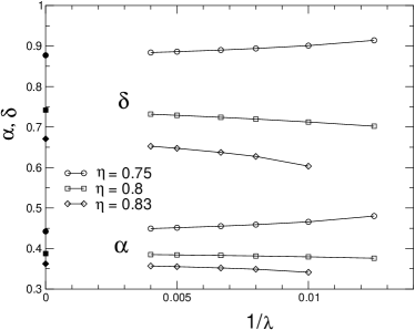
It is easy to check that the above formulas give the correct lattice parameters at the endpoints of the phase IVB region, namely we have $(\alpha=1/2,\delta=1)$ at $\eta=1/\sqrt{2}$ (phase III) and $(\alpha=1/3,\delta=1/\sqrt{3})$ at $\eta=2/3^{3/4}$ (phase V). We did not find in the literature the above specification of the structural parameters of phase IVB in the hard-spheres limit. The numerical test of the results for phase IV parameters is depicted in Fig. 14. For a given $\eta$, the dependence of the parameters $\delta$ (top set) and $\alpha$ (bottom set) on $1/\lambda$, obtained by numerics, is represented by open symbols (connected by solid line), the asymptotic $\lambda\to\infty$ result given by our Eqs. (61) is depicted by full symbol. It is seen that numerical data converge quickly to their asymptotic values.

Figure 14: The structure parameters $\delta$ and $\alpha$ of phase IVB vs. $\lambda$ for three values of $\eta=0.75,0.8,0.83$. Numerical data are represented by open symbols (connected by solid lines), the asymptotic $\lambda\to\infty$ result given by Eqs. (61) is depicted by full symbol.

X Conclusion

In this paper, we have studied the zero-temperature phase diagram of bilayer Wigner crystals of Yukawa particles. To calculate the energy per particle of the phases, we used the recent method of lattice summations Samaj1 extended to Yukawa potentials. The weak point of the method is that one has to know ahead the possible phases from numerical simulations. The strong point is that the truncation of the series of the generalized Misra functions provides extremely precise estimates of the energy, e.g. the truncation at the 5th term provides the accuracy within 17 decimal digits.

Another strong point of Misra functions is that they can be readily expanded around the critical point, providing in this way closed-form expressions for the critical lines between phases II-III (25) and III-IVA (42). Only few Misra functions contribute in the equations for the critical lines in the asymptotic Coulomb $\lambda\to 0$ and hard-spheres $\lambda\to\infty$ limits. The characteristic feature of the Coulomb limit is the parabolic shape of the critical lines, see Eq. (35) with the corresponding plot in Fig. 6 for the II-III phase transition and Eq. (44) with the corresponding plot in Fig. 8 for the III-IVA phase transition. In the hard-spheres limit, the asymptotic formulas for the II-III phase transition (39) and the III-IVA phase transition (47) are pictures by dash-dotted lines in Fig. 7. It turns out that the second-order phase transitions II-III and III-IVA exhibit the mean-field critical exponents (33).

The most important features of the Yukawa phase diagram obtained by Messina and Löwen Messina were confirmed. On the contrary to previous suggestions, phase I goes directly to phase II at $\eta=0$, i.e. there does not exist a finite interval of positive $\eta$-values where phase I dominates. Another important novelty is that instead of the suggested region of phase coexistence, we found a narrow channel within one continuous region of phase IVA. This fact also lead to the tricritical point where the phases IVA, IVB and V meet.

Another application of our formalism is the determination of the structure parameters of soft phases II and IVB in and close to the hard-spheres limit. For $\lambda\to\infty$, the $\eta$-dependence of the aspect ratio $\Delta$ of phase II has already been known Messina , see Eq. (53). We were able to derive the first $1/\lambda$ correction to this asymptotic relation, see Eqs. (56) and (58), which is in perfect agreement with the numerical results (Fig. 13). The derivation of the $\eta$-dependence of two structure parameters $\delta$ and $\alpha$ of phase IVB in the limit $\lambda\to\infty$, see the relations (60) and Fig. 14, is likely new as well.

As concerns future perspectives to apply our method to other systems, the system of particles with $1/r^{\sigma}$ interactions Mazars11 seems to be a good candidate.

Appendix A

We give explicit analytic formulas for several $z_{\nu}(x,y)$ functions (17) with half-integer arguments:

$$z_{1/2}(x,y) = \sqrt{\frac{\pi}{x}}{\rm e}^{-2\sqrt{xy}}\left[1-\frac{1}{2}\ {\rm erfc}{\left(\sqrt{\frac{x}{\pi}}-\sqrt{\pi y}\right)}-\frac{1}{2}{\rm e}^{4\sqrt{xy}}\ {\rm erfc}{\left(\sqrt{\frac{x}{\pi}}+\sqrt{\pi y}\right)}\right],$$ (66)

$$z_{3/2}(x,y) = \sqrt{\frac{\pi}{y}}{\rm e}^{-2\sqrt{xy}}\left[1-\frac{1}{2}\ {\rm erfc}{\left(\sqrt{\frac{x}{\pi}}-\sqrt{\pi y}\right)}+\frac{1}{2}{\rm e}^{4\sqrt{xy}}\ {\rm erfc}{\left(\sqrt{\frac{x}{\pi}}+\sqrt{\pi y}\right)}\right],$$ (67)

$$z_{5/2}(x,y) = \frac{\sqrt{\pi x}}{y}{\rm e}^{-2\sqrt{xy}}\left(1+\frac{1}{2\sqrt{xy}}\right)-\frac{\sqrt{\pi}}{4y^{3/2}}\bigg{[}-4{\rm e}^{-x/\pi-\pi y}\sqrt{y}$$ (68)

$$+{\rm e}^{-2\sqrt{xy}}\left(1+2\sqrt{xy}\right)\ {\rm erfc}{\left(\sqrt{\frac{x}{\pi}}-\sqrt{\pi y}\right)}+{\rm e}^{2\sqrt{xy}}\left(-1+2\sqrt{xy}\right)\ {\rm erfc}{\left(\sqrt{\frac{x}{\pi}}+\sqrt{\pi y}\right)}\bigg{]},$$

$$z_{7/2}(x,y) = \sqrt{\frac{\pi}{y^{3}}}\ x{\rm e}^{-2\sqrt{xy}}\left(1+\frac{3}{2\sqrt{xy}}+\frac{3}{4xy}\right)-\frac{\sqrt{\pi}}{8y^{5/2}}\left[-4{\rm e}^{-x/\pi-\pi y}(3+2\pi y)\sqrt{y}\right.$$ (69)

$$\left.+{\rm e}^{-2\sqrt{xy}}\left(4xy+6\sqrt{xy}+3\right)\ {\rm erfc}{\left(\sqrt{\frac{x}{\pi}}-\sqrt{\pi y}\right)}-{\rm e}^{2\sqrt{xy}}\left(4xy-6\sqrt{xy}+3\right)\ {\rm erfc}{\left(\sqrt{\frac{x}{\pi}}+\sqrt{\pi y}\right)}\right].$$

Here, we introduced the complementary error function Gradshteyn

$${\rm erfc}(z)=\frac{2}{\sqrt{\pi}}\int_{z}^{\infty}\exp{(-t^{2})}\ {\rm d}t.$$ (70)

The case $\nu=1/2$ can be found at the end of Ref. Chaudhry . The expressions for larger $\nu$ can be obtained by applying the obvious relation

$$\frac{\partial z_{\nu}(x,y)}{\partial y}=-z_{\nu+1}(x,y).$$ (71)

The Misra function case $z_{\nu}(0,y)$ Misra should be understood in the sense of the limit $x\to 0$,

$$z_{1/2}(0,y) = \frac{2}{\sqrt{\pi}}\left[{\rm e}^{-\pi y}-\pi\sqrt{y}\ {\rm erfc}{\left(\sqrt{\pi y}\right)}\right],$$

$$z_{3/2}(0,y) = \sqrt{\frac{\pi}{y}}\ {\rm erfc}{\left(\sqrt{\pi y}\right)},$$

$$z_{5/2}(0,y) = \frac{\sqrt{\pi}}{2y^{3/2}}\left[2{\rm e}^{-\pi y}\sqrt{y}\ +{\rm erfc}{\left(\sqrt{\pi y}\right)}\right],$$

$$z_{7/2}(0,y) = \frac{\sqrt{\pi}}{4y^{5/2}}\bigg{[}2{\rm e}^{-\pi y}\sqrt{y}\left(3+2\pi y\right)$$ (72)

$$+3\ {\rm erfc}{\left(\sqrt{\pi y}\right)}\bigg{]}.$$

We need also the asymptotic expansions of $z_{\nu}(x,y)$ when one of the arguments $x$ or $y$ is large. For $x$ finite and $y\gg 1$, we get

$$z_{1/2}(x,y) = \frac{{\rm e}^{-\pi y-x/\pi}}{y\pi^{3/2}}\left[1+{\cal O}\left(\frac{1}{y}\right)\right],$$

$$z_{3/2}(x,y) = \frac{{\rm e}^{-\pi y-x/\pi}}{y\sqrt{\pi}}\left[1+{\cal O}\left(\frac{1}{y}\right)\right],$$

$$z_{5/2}(x,y) = \sqrt{\pi}\frac{{\rm e}^{-\pi y-x/\pi}}{y}\left[1+{\cal O}\left(\frac{1}{y}\right)\right],$$

$$z_{7/2}(x,y) = \sqrt{\pi^{3}}\frac{{\rm e}^{-\pi y-x/\pi}}{y}\left[1+{\cal O}\left(\frac{1}{y}\right)\right].$$ (73)

For $y$ finite and $x\gg 1$, we have

$$z_{1/2}(x,y) = \sqrt{\frac{\pi}{x}}{\rm e}^{-2\sqrt{xy}}+{\cal O}\left(\frac{1}{x}{\rm e}^{-x/\pi}\right),$$

$$z_{3/2}(x,y) = \sqrt{\frac{\pi}{y}}{\rm e}^{-2\sqrt{xy}}+{\cal O}\left(\frac{1}{x}{\rm e}^{-x/\pi}\right),$$

$$z_{5/2}(x,y) = \frac{\sqrt{\pi x}}{y}{\rm e}^{-2\sqrt{xy}}\left(1+\frac{1}{2\sqrt{xy}}\right)+{\cal O}\left(\frac{1}{x}{\rm e}^{-x/\pi}\right),$$

$$z_{7/2}(x,y) = \sqrt{\frac{\pi}{y^{3}}}\ x{\rm e}^{-2\sqrt{xy}}\left(1+\frac{3}{2\sqrt{xy}}+\frac{3}{4xy}\right)$$ (74)

$$+{\cal O}\left(\frac{1}{x}{\rm e}^{-x/\pi}\right).$$

We applied the large-argument expansion of the error function Gradshteyn , erfc$(z)\approx\exp({-z^{2}})/(\sqrt{\pi}z)$.

For small arguments $\delta x$ and $\delta y$, we shall need the following expansion

$$z_{\nu}\left(x+\delta x,y+\delta y\right)=\int_{0}^{1/\pi}\frac{{\rm d}t}{t^{\nu}}{\rm e}^{-(x+\delta x)t}{\rm e}^{-(y+\delta y)/t}$$

$$\approx\int_{0}^{1/\pi}\frac{{\rm d}t}{t^{\nu}}{\rm e}^{-xt}{\rm e}^{-y/t}(1-\delta x\ t)(1-\delta y/t)$$

$$\approx z_{\nu}(x,y)-\delta x\ z_{\nu-1}(x,y)-\delta y\ z_{\nu+1}(x,y),\phantom{aa}$$ (75)

where we kept only terms linear in small variables.

Appendix B

The coefficients $f_{1,2}(\eta,\lambda)$ in Eq. (18) are given by

$$f_{1}(\eta,\lambda) = \frac{\eta}{2\sqrt{\pi}\lambda}\Bigg{\{}2\sum_{j=1}^{\infty}\left[j^{2}z_{5/2}\left(0,\frac{\lambda^{2}}{4\pi^{2}\eta^{2}}+j^{2}\sqrt{3}\right)-\frac{j^{2}}{3}z_{5/2}\left(0,\frac{\lambda^{2}}{4\pi^{2}\eta^{2}}+\frac{j^{2}}{\sqrt{3}}\right)\right]$$ (76)

$$+4\sum_{j,k=1}^{\infty}\left(k^{2}-\frac{j^{2}}{3}\right)z_{5/2}\left(0,\frac{\lambda^{2}}{4\pi^{2}\eta^{2}}+\frac{j^{2}}{\sqrt{3}}+k^{2}\sqrt{3}\right)$$

$$2\sum_{j=1}^{\infty}(-1)^{j}\left[j^{2}z_{5/2}\left(\pi^{2}\eta^{2},\frac{\lambda^{2}}{4\pi^{2}\eta^{2}}+j^{2}\sqrt{3}\right)-\frac{j^{2}}{3}z_{5/2}\left(\pi^{2}\eta^{2},\frac{\lambda^{2}}{4\pi^{2}\eta^{2}}+\frac{j^{2}}{\sqrt{3}}\right)\right]$$

$$+4\sum_{j,k=1}^{\infty}(-1)^{j}(-1)^{k}\left(k^{2}-\frac{j^{2}}{3}\right)z_{5/2}\left(\pi^{2}\eta^{2},\frac{\lambda^{2}}{4\pi^{2}\eta^{2}}+\frac{j^{2}}{\sqrt{3}}+k^{2}{\sqrt{3}}\right)$$

$$+2\sum_{j=1}^{\infty}\left[j^{2}z_{5/2}\left(\frac{\lambda^{2}}{4\eta^{2}},j^{2}\sqrt{3}\right)-\frac{j^{2}}{3}z_{5/2}\left(\frac{\lambda^{2}}{4\eta^{2}},\frac{j^{2}}{\sqrt{3}}\right)\right]$$

$$+4\sum_{j,k=1}^{\infty}\left(k^{2}-\frac{j^{2}}{3}\right)z_{5/2}\left(\frac{\lambda^{2}}{4\eta^{2}},\frac{j^{2}}{\sqrt{3}}+k^{2}{\sqrt{3}}\right)$$

$$4\sum_{j,k=1}^{\infty}\left[(k-1/2)^{2}-\frac{(j-1/2)^{2}}{3}\right]z_{5/2}\left[\frac{\lambda^{2}}{4\eta^{2}},\eta^{2}+\frac{(j-1/2)^{2}}{\sqrt{3}}+(k-1/2)^{2}\sqrt{3}\right]\Bigg{\}},$$

$$f_{2}(\eta,\lambda) = \frac{\eta}{2\sqrt{\pi}\lambda}\Bigg{(}2\sum_{j=1}^{\infty}\left[\frac{j^{4}}{18}z_{7/2}\left(0,\frac{\lambda^{2}}{4\pi^{2}\eta^{2}}+\frac{j^{2}}{\sqrt{3}}\right)+\frac{j^{4}}{2}z_{7/2}\left(0,\frac{\lambda^{2}}{4\pi^{2}\eta^{2}}+j^{2}\sqrt{3}\right)-\frac{j^{2}}{3\sqrt{3}}z_{5/2}\left(0,\frac{\lambda^{2}}{4\pi^{2}\eta^{2}}+\frac{j^{2}}{\sqrt{3}}\right)\right]$$ (77)

$$+4\sum_{j,k=1}^{\infty}\left[\frac{1}{2}\left(k^{2}-\frac{j^{2}}{3}\right)^{2}z_{7/2}\left(0,\frac{\lambda^{2}}{4\pi^{2}\eta^{2}}+\frac{j^{2}}{\sqrt{3}}+k^{2}\sqrt{3}\right)-\frac{j^{2}}{3\sqrt{3}}z_{5/2}\left(0,\frac{\lambda^{2}}{4\pi^{2}\eta^{2}}+\frac{j^{2}}{\sqrt{3}}+k^{2}\sqrt{3}\right)\right]$$

$$+2\sum_{j=1}^{\infty}(-1)^{j}\bigg{[}\frac{j^{4}}{18}z_{7/2}\left(\pi^{2}\eta^{2},\frac{\lambda^{2}}{4\pi^{2}\eta^{2}}+\frac{j^{2}}{\sqrt{3}}\right)+\frac{j^{4}}{2}z_{7/2}\left(\pi^{2}\eta^{2},\frac{\lambda^{2}}{4\pi^{2}\eta^{2}}+j^{2}\sqrt{3}\right)$$

$$-\frac{j^{2}}{3\sqrt{3}}z_{5/2}\left(\pi^{2}\eta^{2},\frac{\lambda^{2}}{4\pi^{2}\eta^{2}}+\frac{j^{2}}{\sqrt{3}}\bigg{)}\right]$$

$$+4\sum_{j,k=1}^{\infty}(-1)^{j}(-1)^{k}\bigg{[}\frac{1}{2}\left(k^{2}-\frac{j^{2}}{3}\right)^{2}z_{7/2}\left(\pi^{2}\eta^{2},\frac{\lambda^{2}}{4\pi^{2}\eta^{2}}+\frac{j^{2}}{\sqrt{3}}+k^{2}{\sqrt{3}}\right)$$

$$-\frac{j^{2}}{3\sqrt{3}}z_{5/2}\left(\pi^{2}\eta^{2},\frac{\lambda^{2}}{4\pi^{2}\eta^{2}}+\frac{j^{2}}{\sqrt{3}}+k^{2}{\sqrt{3}}\right)\bigg{]}$$

$$2\sum_{j=1}^{\infty}\bigg{[}\frac{j^{4}}{18}z_{7/2}\left(\frac{\lambda^{2}}{4\eta^{2}},\frac{j^{2}}{\sqrt{3}}\right)+\frac{j^{4}}{2}z_{7/2}\left(\frac{\lambda^{2}}{4\eta^{2}},j^{2}\sqrt{3}\right)-\frac{j^{2}}{3\sqrt{3}}z_{5/2}\left(\frac{\lambda^{2}}{4\eta^{2}},\frac{j^{2}}{\sqrt{3}}\right)\bigg{]}$$

$$+4\sum_{j,k=1}^{\infty}\bigg{[}\frac{1}{2}\left(k^{2}-\frac{j^{2}}{3}\right)^{2}z_{7/2}\left(\frac{\lambda^{2}}{4\eta^{2}},\frac{j^{2}}{\sqrt{3}}+k^{2}{\sqrt{3}}\right)-\frac{j^{2}}{3\sqrt{3}}z_{5/2}\left(\frac{\lambda^{2}}{4\eta^{2}},\frac{j^{2}}{\sqrt{3}}+k^{2}{\sqrt{3}}\right)\bigg{]}$$

$$4\sum_{j,k=1}^{\infty}\bigg{\{}\frac{1}{2}\left[(k-1/2)^{2}-\frac{(j-1/2)^{2}}{3}\right]^{2}z_{7/2}\left[\frac{\lambda^{2}}{4\eta^{2}},\eta^{2}+\frac{(j-1/2)^{2}}{\sqrt{3}}+(k-1/2)^{2}\sqrt{3}\right]$$

$$-\frac{(j-1/2)^{2}}{3\sqrt{3}}z_{5/2}\left[\frac{\lambda^{2}}{4\eta^{2}},\eta^{2}+\frac{(j-1/2)^{2}}{\sqrt{3}}+(k-1/2)^{2}\sqrt{3}\right]\bigg{\}}\Bigg{)}.$$

We are interested in the small-$\eta$ behavior of the above functions. One of the arguments in the $z_{\nu}(x,y)$ functions becomes large, thus we can apply the asymptotic relations (73) and (74). Neglecting the exponentially small terms we find that only the seventh and the ninth (last) sums both in (76) and (77) contribute, namely the leading terms with $j=1$ and $j=k=1$, respectively. Consequently, for a fixed $\lambda>0$ and $\eta\to 0$ (i.e. $\lambda/\eta\gg 1$), we have

$$f_{1}(\eta,\lambda) \approx \frac{\eta}{2\sqrt{\pi}\lambda}\left[-\frac{2}{3}z_{5/2}\left(\frac{\lambda^{2}}{4\eta^{2}},\frac{1}{\sqrt{3}}\right)+\frac{2}{3}z_{5/2}\left(\frac{\lambda^{2}}{4\eta^{2}},\eta^{2}+\frac{1}{\sqrt{3}}\right)\right]\approx-\frac{1}{2\sqrt{3}}{\rm e}^{-\frac{\lambda}{3^{1/4}\eta}}+\frac{1}{6\left(\eta^{2}+\frac{1}{\sqrt{3}}\right)}{\rm e}^{-\frac{\lambda}{\eta}\sqrt{\eta^{2}+\frac{1}{\sqrt{3}}}},$$

$$f_{2}(\eta,\lambda) \approx \frac{\eta}{2\sqrt{\pi}\lambda}\left[\frac{1}{9}z_{7/2}\left(\frac{\lambda^{2}}{4\eta^{2}},\frac{1}{\sqrt{3}}\right)+\frac{1}{18}z_{7/2}\left(\frac{\lambda^{2}}{4\eta^{2}},\eta^{2}+\frac{1}{\sqrt{3}}\right)\right]$$ (78)

$$\approx -\frac{\lambda}{8\ 3^{5/4}\eta}{\rm e}^{-\frac{\lambda}{3^{1/4}\eta}}+\frac{\lambda}{144\eta(\eta^{2}+\frac{1}{\sqrt{3}})^{3/2}}{\rm e}^{-\frac{\lambda}{\eta}\sqrt{\eta^{2}+\frac{1}{\sqrt{3}}}},$$

where we repeatedly neglected subleading terms. Expanding also the second exponential $\exp[-\lambda\sqrt{1+\sqrt{3}\eta^{2}}/(3^{1/4}\eta)]$ in $\eta$, we get (22).

Appendix C

The coefficient $g_{2}(\eta,\lambda)$ in Eq. (24) takes the form

$$g_{2}(\eta,\lambda) = \frac{\eta}{\sqrt{\pi}\lambda}\Bigg{(}\sum_{j=1}^{\infty}\left[j^{4}z_{7/2}\left(0,\frac{\lambda^{2}}{4\pi^{2}\eta^{2}}+j^{2}\right)-j^{2}z_{5/2}\left(0,\frac{\lambda^{2}}{4\pi^{2}\eta^{2}}+j^{2}\right)\right]$$ (79)

$$+\sum_{j,k=1}^{\infty}\left[(j^{2}-k^{2})^{2}z_{7/2}\left(0,\frac{\lambda^{2}}{4\pi^{2}\eta^{2}}+j^{2}+k^{2}\right)-(j^{2}+k^{2})z_{5/2}\left(0,\frac{\lambda^{2}}{4\pi^{2}\eta^{2}}+j^{2}+k^{2}\right)\right]$$

$$+\sum_{j=1}^{\infty}(-1)^{j}\left[j^{4}z_{7/2}\left(\pi^{2}\eta^{2},\frac{\lambda^{2}}{4\pi^{2}\eta^{2}}+j^{2}\right)-j^{2}z_{5/2}\left(\pi^{2}\eta^{2},\frac{\lambda^{2}}{4\pi^{2}\eta^{2}}+j^{2}\right)\right]$$

$$+\sum_{j,k=1}^{\infty}(-1)^{j}(-1)^{k}\left[(j^{2}-k^{2})^{2}z_{7/2}\left(\pi^{2}\eta^{2},\frac{\lambda^{2}}{4\pi^{2}\eta^{2}}+j^{2}+k^{2}\right)-(j^{2}+k^{2})z_{5/2}\left(\pi^{2}\eta^{2},\frac{\lambda^{2}}{4\pi^{2}\eta^{2}}+j^{2}+k^{2}\right)\right]$$

$$+\sum_{j=1}^{\infty}\left[j^{4}z_{7/2}\left(\frac{\lambda^{2}}{4\eta^{2}},j^{2}\right)-j^{2}z_{5/2}\left(\frac{\lambda^{2}}{4\eta^{2}},j^{2}\right)\right]$$

$$+\sum_{j,k=1}^{\infty}\left[(j^{2}-k^{2})^{2}z_{7/2}\left(\frac{\lambda^{2}}{4\eta^{2}},j^{2}+k^{2}\right)-(j^{2}+k^{2})z_{5/2}\left(\frac{\lambda^{2}}{4\eta^{2}},j^{2}+k^{2}\right)\right]$$

$$+\sum_{j,k=1}^{\infty}\bigg{\{}\left[(j-1/2)^{2}-(k-1/2)^{2}\right]^{2}z_{7/2}\left[\frac{\lambda^{2}}{4\eta^{2}},\eta^{2}+(j-1/2)^{2}+(k-1/2)^{2}\right]$$

$$-\left[(j-1/2)^{2}+(k-1/2)^{2}\right]z_{5/2}\left[\frac{\lambda^{2}}{4\eta^{2}},\eta^{2}+(j-1/2)^{2}+(k-1/2)^{2}\right]\bigg{\}}\Bigg{)}.$$

Our next step is to analyze the small $\lambda$ behavior of the critical line between phases II-III which is given by $g_{2}(\eta,\lambda)=0$; here, we write $(\eta,\lambda)$ instead of $(\eta^{c},\lambda^{c})$ to simplify the notation. There are two small quantities: $\lambda^{2}$ and $\eta-\eta_{0}$, where we denote the Coulomb transition distance $\eta^{c}(0)\equiv\eta_{0}\approx 0.262760268246823\ldots$. Applying formula (75), we demonstrate one specific example of the expansion of the generalized Misra functions in (79), up to terms linear in small variables $\lambda^{2}$ and $\eta-\eta_{0}$:

$$z_{7/2}\left(\pi^{2}\eta^{2},\frac{\lambda^{2}}{4\pi^{2}\eta^{2}}+j^{2}\right)\approx z_{7/2}\left(\pi^{2}\eta_{0}^{2},j^{2}\right)-\frac{\lambda^{2}}{4\pi^{2}\eta_{0}^{2}}z_{9/2}\left(\pi^{2}\eta_{0}^{2},j^{2}\right)-2\pi^{2}\eta_{0}(\eta-\eta_{0})z_{5/2}\left(\pi^{2}\eta_{0}^{2},j^{2}\right).$$ (80)

Here, we used that $\eta^{2}=[\eta_{0}+(\eta-\eta_{0})]^{2}\approx\eta_{0}^{2}+2\eta_{0}(\eta-\eta_{0})$. The absolute terms, like the leading one on the r.h.s. of (80), are canceled by the definition of the critical point at $\lambda=0$: $g_{2}(\eta_{0},0)=0$. Thus we are left with

$$c_{1}^{(23)}\lambda^{2}+c_{2}^{(23)}(\eta-\eta_{0})=0,$$ (81)

where

$$c_{1}^{(23)} = -\sum_{j=1}^{\infty}\left[j^{4}z_{9/2}\left(0,j^{2}\right)-j^{2}z_{7/2}\left(0,j^{2}\right)\right]/(4\pi^{2}\eta_{0}^{2})$$ (82)

$$-\sum_{j,k=1}^{\infty}\left[(j^{2}-k^{2})^{2}z_{9/2}\left(0,j^{2}+k^{2}\right)-(j^{2}+k^{2})z_{7/2}\left(0,j^{2}+k^{2}\right)\right]/(4\pi^{2}\eta_{0}^{2})$$

$$-\sum_{j=1}^{\infty}(-1)^{j}\left[j^{4}z_{9/2}\left(\pi^{2}\eta_{0}^{2},j^{2}\right)-j^{2}z_{7/2}\left(\pi^{2}\eta_{0}^{2},j^{2}\right)\right]/(4\pi^{2}\eta_{0}^{2})$$

$$-\sum_{j,k=1}^{\infty}(-1)^{j}(-1)^{k}\left[(j^{2}-k^{2})^{2}z_{9/2}\left(\pi^{2}\eta_{0}^{2},j^{2}+k^{2}\right)-(j^{2}+k^{2})z_{7/2}\left(\pi^{2}\eta_{0}^{2},j^{2}+k^{2}\right)\right]/(4\pi^{2}\eta_{0}^{2})$$

$$-\sum_{j=1}^{\infty}\left[j^{4}z_{5/2}\left(0,j^{2}\right)-j^{2}z_{3/2}\left(0,j^{2}\right)\right]/(4\eta_{0}^{2})$$

$$-\sum_{j,k=1}^{\infty}\left[(j^{2}-k^{2})^{2}z_{5/2}\left(0,j^{2}+k^{2}\right)-(j^{2}+k^{2})z_{3/2}\left(0,j^{2}+k^{2}\right)\right]/(4\eta_{0}^{2})$$

$$-\sum_{j,k=1}^{\infty}\bigg{\{}\left[(j-1/2)^{2}-(k-1/2)^{2}\right]^{2}z_{5/2}\left[0,\eta_{0}^{2}+(j-1/2)^{2}+(k-1/2)^{2}\right]$$

$$+\left[(j-1/2)^{2}+(k-1/2)^{2}\right]z_{3/2}\left[0,\eta_{0}^{2}+(j-1/2)^{2}+(k-1/2)^{2}\right]\bigg{\}}/(4\eta_{0}^{2})\approx-0.04791591901052$$

and

$$c_{2}^{(23)} = -\sum_{j=1}^{\infty}(-1)^{j}\left[j^{4}z_{5/2}\left(\pi^{2}\eta_{0}^{2},j^{2}\right)-j^{2}z_{3/2}\left(\pi^{2}\eta_{0}^{2},j^{2}\right)\right]2\pi^{2}\eta_{0}$$ (83)

$$-\sum_{j,k=1}^{\infty}(-1)^{j}(-1)^{k}\left[(j^{2}-k^{2})^{2}z_{5/2}\left(\pi^{2}\eta_{0}^{2},j^{2}+k^{2}\right)-(j^{2}+k^{2})z_{3/2}\left(\pi^{2}\eta_{0}^{2},j^{2}+k^{2}\right)\right]2\pi^{2}\eta_{0}$$

$$-\sum_{j,k=1}^{\infty}\bigg{\{}\left[(j-1/2)^{2}-(k-1/2)^{2}\right]^{2}z_{9/2}\left[0,\eta_{0}^{2}+(j-1/2)^{2}+(k-1/2)^{2}\right]$$

$$+\left[(j-1/2)^{2}+(k-1/2)^{2}\right]z_{7/2}\left[0,\eta_{0}^{2}+(j-1/2)^{2}+(k-1/2)^{2}\right]\bigg{\}}2\eta_{0}\approx 1.15830861669576.$$

Eq. (81) with the specified constants yields (35).

Appendix D

The function $h_{2}(\eta,\lambda)$ in Eq. (41) reads as follows

$$h_{2}(\eta,\lambda) = \frac{\eta}{2\sqrt{2\pi}\lambda}\Bigg{(}\sum_{j=1}^{\infty}\left[1+(-1)^{j}\right]\left[j^{4}z_{7/2}\left(0,\frac{\lambda^{2}}{2\pi^{2}\eta^{2}}+j^{2}\right)-j^{2}z_{5/2}\left(0,\frac{\lambda^{2}}{2\pi^{2}\eta^{2}}+j^{2}\right)\right]$$ (84)

$$+\sum_{j,k=1}^{\infty}\left[1+(-1)^{j}(-1)^{k}\right]\left[(j^{2}-k^{2})^{2}z_{7/2}\left(0,\frac{\lambda^{2}}{2\pi^{2}\eta^{2}}+j^{2}+k^{2}\right)-(j^{2}+k^{2})z_{5/2}\left(0,\frac{\lambda^{2}}{2\pi^{2}\eta^{2}}+j^{2}+k^{2}\right)\right]$$

$$+\sum_{j=1}^{\infty}\left[1+(-1)^{j}\right]\left[j^{4}z_{7/2}\left(\eta^{2}\pi^{2}/2,\frac{\lambda^{2}}{2\pi^{2}\eta^{2}}+j^{2}\right)-j^{2}z_{5/2}\left(\eta^{2}\pi^{2}/2,\frac{\lambda^{2}}{2\pi^{2}\eta^{2}}+j^{2}\right)\right]$$

$$+2\sum_{j,k=1}^{\infty}(-1)^{j}\left[(j^{2}-k^{2})^{2}z_{7/2}\left(\frac{\eta^{2}\pi^{2}}{2},\frac{\lambda^{2}}{2\pi^{2}\eta^{2}}+j^{2}+k^{2}\right)-(j^{2}+k^{2})z_{5/2}\left(\frac{\eta^{2}\pi^{2}}{2},\frac{\lambda^{2}}{2\pi^{2}\eta^{2}}+j^{2}+k^{2}\right)\right]$$

$$+\sum_{j=1}^{\infty}\left[j^{4}z_{7/2}\left(\frac{\lambda^{2}}{2\eta^{2}},j^{2}\right)-j^{2}z_{5/2}\left(\frac{\lambda^{2}}{2\eta^{2}},j^{2}\right)\right]$$

$$+\sum_{j,k=1}^{\infty}\left[(j^{2}-k^{2})^{2}z_{7/2}\left(\frac{\lambda^{2}}{2\eta^{2}},j^{2}+k^{2}\right)-(j^{2}+k^{2})z_{5/2}\left(\frac{\lambda^{2}}{2\eta^{2}},j^{2}+k^{2}\right)\right]$$

$$+\sum_{j,k=1}^{\infty}\bigg{\{}\left[(j-1/2)^{2}-(k-1/2)^{2}\right]^{2}z_{7/2}\left[\frac{\lambda^{2}}{2\eta^{2}},(j-1/2)^{2}+(k-1/2)^{2}\right]$$

$$-\left[(j-1/2)^{2}+(k-1/2)^{2}\right]z_{5/2}\left[\frac{\lambda^{2}}{2\eta^{2}},(j-1/2)^{2}+(k-1/2)^{2}\right]\bigg{\}}$$

$$+2\sum_{j,k=1}^{\infty}\bigg{\{}\left[(j-1/2)^{2}-k^{2}\right]^{2}z_{7/2}\left[\frac{\lambda^{2}}{2\eta^{2}},\frac{\eta^{2}}{2}+(j-1/2)^{2}+k^{2}\right]$$

$$-\left[(j-1/2)^{2}+k^{2}\right]z_{5/2}\left[\frac{\lambda^{2}}{2\eta^{2}},\frac{\eta^{2}}{2}+(j-1/2)^{2}+k^{2}\right]\bigg{\}}$$

$$+\sum_{j=1}^{\infty}\left\{(j-1/2)^{4}z_{7/2}\left[\frac{\lambda^{2}}{2\eta^{2}},\frac{\eta^{2}}{2}+(j-1/2)^{2}\right]-(j-1/2)^{2}z_{5/2}\left[\frac{\lambda^{2}}{2\eta^{2}},\frac{\eta^{2}}{2}+(j-1/2)^{2}\right]\right\}\Bigg{)}.$$

Now we can analyze the low-$\lambda$ limit of the critical line between phases III and IVA. Proceeding in the same way as in the previous case of the II-III transition, taking the value $\eta_{0}=\eta^{c}(0)\approx 0.621480924579783$, we get from (84) the equality

$$c_{1}^{(34)}\lambda^{2}+c_{2}^{(34)}(\eta-\eta_{0})=0$$ (85)

with $c_{1}^{(34)}\approx 0.0063328359292865$ and $c_{2}^{(34)}\approx-0.94855575801235884369$, so that Eq. (44) follows.

References

- (1) A. W. C. Lau, D. Levine, and P. Pincus, Phys. Rev. Lett. 84, 4116 (2000); A. W. C. Lau, P. Pincus, D. Levine, and H. A. Fertig, Phys. Rev. E 63, 051604 (2001).
- (2) A. Y. Grosberg, T. T. Nguyen, and B. I. Shklovskii, Rev. Mod. Phys. 74, 329 (2002).
- (3) Y. Levin, Rep. Prog. Phys. 65, 1577 (2002).
- (4) A. Naji, S. Jungblut, A. G. Moreira, and R. R. Netz, Physica A 352, 131 (2005).
- (5) L. Šamaj and E. Trizac, Phys. Rev. Lett. 106, 078301 (2011); Phys. Rev. E 84, 041401 (2011); Contrib. Plasma Phys. 52, 53 (2012).
- (6) D. V. Fil, Low Temp. Phys. 27, 384 (2001); Y. P. Chen, Phys. Rev. B 73, 115314 (2006).
- (7) H. Imamura, P. A. Maksym, and H. Aoki, Phys. Rev. B 53, 12613 (1996).
- (8) L. W. Teng, P. S. Tu, and L. I, Phys. Rev. Lett. 90, 145004 (2003).
- (9) A. Reinmüller, E. C. Oǧuz, R. Messina, H. Löwen, H. J. Schöpe, and T. Palberg, European Phys. J. 222, 3011 (2013); R. Messina, J. Phys.: Condens. Matter 21, 113102 (2009).
- (10) S. Earnshaw, Trans. Camb. Phil. Soc., 7, 97 (1842).
- (11) V. I. Falko, Phys. Rev. B 49, 7774 (1994).
- (12) K. Esfarjani and Y. Kawazoe, J. Phys.: Condens. Matter 7, 7217 (1995).
- (13) G. Goldoni and F.M. Peeters, Phys. Rev. B 53, 4591 (1996).
- (14) I. V. Schweigert, V. A. Schweigert and F. M. Peeters, Phys. Rev. Lett. 82, 5293 (1999); Phys. Rev. B 60, 14665 (1999).
- (15) J. J. Weis, D. Levesque, and S. Jorge, Phys. Rev. B 63, 045308 (2001).
- (16) L. Bonsall and A. A. Maradudin, Phys. Rev. B 15, 1959 (1977).
- (17) L. Šamaj and E. Trizac, Europhys. Lett. 98, 36004 (2012); Phys. Rev. B 85, 205131 (2012).
- (18) S. Nunomura, J. Goree, S. Hu, X. Wang, A. Bhattacharjee and K. Avinash, Phys. Rev. Lett. 89, 035001 (2002).
- (19) C. A. Murray, W. O. Sprenger and R. A. Wenk, Phys. Rev. B 42, 688 (1990).
- (20) M. Schmidt and H. Löwen, Phys. Rev. Lett. 76, 4552 (1996); Phys. Rev. E 55, 7228 (1997).
- (21) S. Neser, C. Bechinger, P. Leiderer, and T. Palberg, Phys. Rev. Lett. 79, 2348 (1997).
- (22) A. Fortini and M. Dijkstra, J. Phys.: Cond. Mat. 18, L371 (2006).
- (23) M. Mazars, Phys. Rep. 500, 43 (2011).
- (24) R. Messina and H. Löwen, Phys. Rev. Lett. 91, 146101 (2003).
- (25) E.C. Oǧuz, R. Messina and H. Löwen, Europhys. Lett. 86, 28002 (2009).
- (26) I. S. Gradshteyn and I. M. Ryzhik, Table of Integrals, Series, and Products, 6th edn. (Academic Press, London, 2000).
- (27) R. D. Misra, Math. Proc. Cambridge Philos. Soc. 36, 173 (1940).
- (28) S.-K. Ma, Modern Theory of Critical Phenomena (Westview Press, New York, 1976).
- (29) M. Mazars, Europhys. Lett. 84, 55002 (2008).
- (30) M. A. Chaudhry, N. M. Temme and E. J. M. Veling, J. Comput. Appl. Math. 67, 371 (1996).