Optimality of Refraction Strategies for Spectrally Negative Lévy Processes

Abstract.

We revisit a stochastic control problem of optimally modifying the underlying spectrally negative Lévy process. A strategy must be absolutely continuous with respect to the Lebesgue measure, and the objective is to minimize the total costs of the running and controlling costs. Under the assumption that the running cost function is convex, we show the optimality of a refraction strategy. We also obtain the convergence of the optimal refraction strategies and the value functions, as the control set is enlarged, to those in the relaxed case without the absolutely continuous assumption. Numerical results are further given to confirm these analytical results.

Key words: stochastic control; refracted Lévy processes; scale functions
AMS 2010 Subject Classifications: 60G51, 93E20, 49J40

1. Introduction

We consider a class of stochastic control problems under the restriction that strategies must be absolutely continuous with respect to the Lebesgue measure. Given a spectrally negative Lévy process, the controller aims to optimally decrease the process so as to minimize the sum of the expected running and controlling costs. The running cost is modeled as a convex function $h$ of the controlled process that is accumulated over time. The controlling cost is proportional to the size of control. Our objective is to show the optimality of the refraction strategy so that the controlled process becomes a refracted Lévy process of Kyprianou and Loeffen [15], with a suitable choice of the refraction boundary level.

In the last decade, there have been great developments in the theory of Lévy processes and its applications in stochastic control. A representative example is its contributions in de Finetti’s optimal dividend problem, where the classical compound Poisson model has been generalized to a spectrally negative Lévy model. The expected net present value (NPV) of total dividends under the reflection strategy, so that the controlled process becomes a reflected Lévy process, can be concisely written in terms of the scale function (see [2]). While the optimality may fail depending on the choice of the Lévy measure, Loeffen [17] obtains a sufficient condition for optimality and in particular shows that it holds when the Lévy measure has a completely monotone density. Other stochastic control problems that have been explicitly solved via the scale function include the dual model of the optimal dividend problem [5], inventory control problems as in [4, 21], and games between two players [11].

While the reflection strategy is commonly shown to be optimal in these papers, implementing it in real life is often not feasible nor realistic. Most likely in every scenario, the ability of controlling is limited and hence is more reasonable to restrict the amount of modification one can make to the underlying process.

In classical settings of the optimal dividend problem, reflection strategies that are shown to be optimal always lead to ruin in finite time; these results have been in dispute and there has been a need for new models so as to avoid these undesirable conclusions. In currency rate control (see, e.g., [12] and [18]), where a central bank controls the currency rate so as to prevent it from going too high or too low, reflection strategies, that are shown to be optimal under many models, are not implementable in real life. In 2011, Swiss central bank introduced the peg so as to stabilize their currency in response to its escalating value against other currencies: they set a ceiling on its rate against Euro, and literally implemented a reflection strategy. However, this only lasted until the beginning of 2015 when they had to admit the enormous cost of doing it and scraped the ceiling.

One way to model these limitations on the control set is to add an extra restriction on the set of admissible strategies to be absolutely continuous with respect to the Lebesgue measure. Kyprianou et al. [16], in particular, consider the optimal dividend problem under this restriction. They show under the completely monotone assumption on the Lévy measure that a refraction strategy is optimal: Roughly speaking, the resulting controlled process becomes a refracted Lévy process that progresses like the original Lévy process below a chosen threshold while it does like a drift-changed process above it.

In this paper, we revisit the stochastic control problem that minimizes the convex running costs. The setting is similar to the existing literature on singular/impulse control problems as in [6], [7] and [21]. The convex assumption is typically needed and is required in, e.g., [3, 9, 20]. Differently from these papers, we consider a version with an additional condition that the strategy is absolutely continuous. More precisely, a strategy must be of the form $L_{t}=\int_{0}^{t}\ell_{s}{\rm d}s$, $t\geq 0$, with $\ell$ restricted to take values in $[0,\delta]$ uniformly in time. As in [16], our objective is to show the optimality of a refraction strategy. While a reflected Lévy process can be dealt relatively easily because it moves just like the original Lévy process except at the times running maximum/minimum is updated, a refracted Lévy process moves in two different ways depending on whether it is above or below the given threshold. The computation thus becomes more intricate.

In order to tackle our problem, we take the following steps.

1. By directly using the resolvent measure for the refracted Lévy process as in [15], we first write the expected NPV of total costs using the scale function under each refraction strategy.

2. The candidate threshold $b^{*}\in[-\infty,\infty]$ is then chosen by observing the identity (3.20) below. We show that such $b^{*}$ is given as a root of a monotone function $I$ defined in (3.23) below, or otherwise it is either $-\infty$ or $\infty$.

3. We then verify the optimality of such strategy. Toward this end, we derive a sufficient condition for optimality (verification lemma), and then show that it is equivalent to certain conditions on the smoothness and slope of the value function. We observe that the level $b^{*}$ is such that the candidate value function becomes smooth and convex; using these facts, we complete the proof of optimality.

It is important to highlight the fact that this set of results are obtained without using directly the HJB equation associated with this control problem and, instead, it is used in an indirect way to derive sufficient conditions for optimality, based only on the derivative of the value function; see Lemmas 4.1 and 4.3.

In addition to solving this problem, we analyze the behavior as the upper bound $\delta$, of the control set, becomes large. Being consistent with our intuition, we show that the optimal refraction strategy of this problem converges to the reflection strategy that has been shown to be optimal in the original problem without the absolutely continuous condition. In particular, we show the convergence of the optimal threshold $b^{*}$ and value function to those obtained in [21]. In order to discuss the practical side of implementing the obtained optimal strategy, we give a series of computational experiments using the phase-type Lévy process and quadratic cost function. We confirm the optimality as well as the convergence as $\delta\uparrow\infty$ to the reflection strategy.

The rest of the paper is organized as follows. The problem is defined in Section 2. In Section 3, we first review the refracted spectrally negative Lévy process and the scale function. We then compute the NPV of total costs under a refraction strategy and choose a candidate refraction boundary level $b^{*}$. Section 4 verifies the optimality of the selected refraction strategy. Section 5 studies the convergence as $\delta\uparrow\infty$ of the optimal refraction strategy to the optimal reflection strategy. We conclude the paper with numerical results in Section 6.

2. Mathematical Model

Let $(\Omega,\mathcal{F},\mathbb{P})$ be a probability space hosting a spectrally negative Lévy process $X=\left\{X_{t};t\geq 0\right\}$ whose Laplace exponent is given by

(2.1) $$\psi(\theta):=\log\mathbb{E}[\mathrm{e}^{\theta X_{1}}]=\gamma\theta+\frac{\sigma^{2}}{2}\theta^{2}+\int_{(-\infty,0)}(\mathrm{e}^{\theta z}-1-\theta z\mathbf{1}_{\{z>-1\})}\nu({\rm d}z),\quad\theta\geq 0,$$

where $\nu$ is a Lévy measure with support in $(-\infty,0)$ and satisfying the integrability condition $\int_{(-\infty,0)}(1\wedge z^{2})\nu({\rm d}z)<\infty$. It has paths of bounded variation if and only if $\sigma=0$ and $\int_{(-1,0)}|z|\,\nu({\rm d}z)<\infty$; in this case, we write (2.1) as

$$\psi(\theta)=\tilde{\gamma}\theta+\int_{(-\infty,0)}(\mathrm{e}^{\theta z}-1)\nu({\rm d}z),\quad\theta\geq 0,$$

with $\tilde{\gamma}:=\gamma-\int_{(-1,0)}z\,\nu({\rm d}z)$. We exclude the case in which $X$ is the negative of a subordinator (i.e., $X$ has monotonically decreasing paths a.s.). This assumption implies that $\tilde{\gamma}>0$ when $X$ is of bounded variation. Let $\mathbb{P}_{x}$ be the conditional probability under which $X_{0}=x$ (also let $\mathbb{P}\equiv\mathbb{P}_{0}$), and let $\mathbb{F}:=\left\{\mathcal{F}_{t};t\geq 0\right\}$ be the filtration generated by $X$.

Fix $\beta\in\mathbb{R}$, $\delta>0$ and a measurable function $h:\mathbb{R}\rightarrow\mathbb{R}$ that is specified in Assumption 2.2 below. Define $\Pi_{\delta}$ as the set of absolutely continuous strategies $\ell$ given by adapted processes $L_{t}=\int_{0}^{t}\ell_{s}{\rm d}s$, $t\geq 0$, with $\ell$ restricted to take values in $[0,\delta]$ uniformly in time. For $q>0$ fixed, the objective is to consider the NPV of the expected total costs

(2.2) $$v_{\ell}(x):=\mathbb{E}_{x}\Big{[}\int_{0}^{\infty}\mathrm{e}^{-qt}(h(U_{t}^{\ell})+\beta\ell_{t}){\rm d}t\Big{]},$$

where

$$U_{t}^{\ell}:=X_{t}-L_{t},\quad t\geq 0,$$

and compute the (optimal) value function

(2.3) $$v(x):=\inf_{{\ell}\in\Pi_{\delta}}v_{\ell}(x),\quad x\in\mathbb{R},$$

as well as the optimal strategy that attains it, if such a strategy exists.

We make the following standing assumptions on the Lévy process $X$ and the running cost function $h$.

Assumption 2.1.

1. For the case $X$ is of bounded variation, we assume that $\tilde{\gamma}-\delta>0$.

2. We assume that there exists $\bar{\theta}>0$ such that $\int_{(-\infty,-1]}\exp(\bar{\theta}|z|)\nu({\rm d}z)<\infty$.

Assumption 2.2.

We assume that $h$ is convex and has at most polynomial growth in the tail. That is to say, there exist $k_{1},k_{2}>0$ and $N\in\mathbb{N}$ such that $h(x)\leq k_{1}+k_{2}|x|^{N}$ for all $x\in\mathbb{R}$ such that $|x|>m$.

Define the drift-changed Lévy process

(2.4) $$Y_{t}:=X_{t}-\delta t,\quad t\geq 0,$$

which is the resulting controlled process if $\ell$ is uniformly set to be the maximal value $\delta$. Assumption 2.1 (1) guarantees that $Y$ is not the negative of a subordinator, and hence is again a spectrally negative Lévy process. This is commonly assumed (see, e.g., [16]) so that the refracted Lévy process given below is well-defined.

By Assumption 2.1 (2), the domain of the Laplace exponent (2.1) can be extended to $(-\bar{\theta},\infty)$ and, by its continuity, we can choose sufficiently small $\theta>0$ such that $\psi(-\theta)<q$. With this choice of $\theta$,

(2.5) $$\mathbb{E}[\mathrm{e}^{-\theta X_{\rm{e}_{q}}}]=q\int_{0}^{\infty}\mathrm{e}^{-qt}\mathbb{E}[\mathrm{e}^{-\theta X_{t}}]{\rm d}t=q\int_{0}^{\infty}\mathrm{e}^{-qt}\mathrm{e}^{\psi(-\theta)t}{\rm d}t<\infty,$$

where $\rm{e}_{q}$ is an independent exponential random variable with parameter $q$.

Assumptions 2.1 (2) and 2.2 guarantee that $v_{\ell}$ as in (2.2) is well-defined and finite for all ${\ell}\in\Pi_{\delta}$. To see this, by the convexity of $h$ and because $Y_{t}\leq U_{t}^{\ell}\leq X_{t}$,

(2.6) $$h(U_{t}^{\ell})\leq h(X_{t})\vee h(Y_{t}),$$

while, with $\underline{h}:=\inf_{x\in\mathbb{R}}h(x)\in[-\infty,\infty)$, we have

(2.9) $$h(U_{t}^{\ell})\geq\left\{\begin{array}[]{ll}\underline{h}&\textrm{if }\underline{h}>-\infty,\\ h(X_{t})\wedge h(Y_{t})&\textrm{otherwise}.\end{array}\right.$$

Hence, for any random time $T$ (independent of $\rm{e}_{q}$),

(2.10) $$\begin{split}\mathbb{E}_{x}\Big{[}\int_{T}^{\infty}\mathrm{e}^{-qt}\sup_{{\ell}\in\Pi_{\delta}}|h(U_{t}^{\ell})|{\rm d}t\Big{]}\leq\mathbb{E}_{x}\Big{[}\int_{T}^{\infty}\mathrm{e}^{-qt}(|h(X_{t})|+|h(Y_{t})|+|\underline{h}|\mathbf{1}_{\{\underline{h}>-\infty\}}){\rm d}t\Big{]}\\ =q^{-1}\mathbb{E}_{x}\Big{[}\mathbf{1}_{\{{\rm{e}_{q}}>T\}}(|h(X_{\rm{e}_{q}})|+|h(Y_{\rm{e}_{q}})|+|\underline{h}|\mathbf{1}_{\{\underline{h}>-\infty\}})\Big{]}<\infty,\end{split}$$

where the finiteness holds by (2.5) and Assumption 2.2. The finiteness (2.10) will be particularly important in the verification step (Lemma 4.1 below). As is commonly used in verification arguments, localization is first needed; (2.10) lets us interchange the limits over integrals.

Remark 2.1.

We can also consider a version of this problem where a linear drift is added to the increments of $X$ (as opposed to being subtracted): one wants to minimize, for some $\tilde{\beta}\in\mathbb{R}$, the NPV

$$\tilde{v}_{\ell}(x):=\mathbb{E}_{x}\Big{[}\int_{0}^{\infty}\mathrm{e}^{-qt}(h(X_{t}+L_{t})+\tilde{\beta}\ell_{t}){\rm d}t\Big{]}.$$

However, it is easy to verify that this problem is equivalent to the problem described above.

To see this, we use $Y$ as in (2.4) and set $\tilde{L}_{t}:=\delta t-L_{t}$ (which is admissible with $\tilde{L}_{t}=\int_{0}^{t}\tilde{\ell}_{s}{\rm d}s$ where $\tilde{\ell}_{s}:=\delta-\ell_{s}\in[0,\delta]$ a.s.). Then, we can write

$$\tilde{v}_{\ell}(x)=\mathbb{E}_{x}\Big{[}\int_{0}^{\infty}\mathrm{e}^{-qt}(h(Y_{t}-\tilde{L}_{t})-\tilde{\beta}\tilde{\ell}_{t}){\rm d}t\Big{]}+\frac{\tilde{\beta}\delta}{q}.$$

Hence it is equivalent to solving our problem for $\beta:=-\tilde{\beta}$.

3. Refraction Strategies

One of the objectives of this paper is to show the optimality of the refraction strategies, say $\ell^{b}\in\Pi_{\delta}$, under which the controlled process becomes the refracted Lévy process $U^{b}=\{U^{b}_{t};t\geq 0\}$ of [15], with a suitable choice of the refraction boundary $b\in\mathbb{R}$. By [15, Theorem 1 and Remark 3], this is a strong Markov process given by the unique strong solution to the SDE

$${\rm d}U_{t}^{b}={\rm d}X_{t}-\delta\mathbf{1}_{\{U_{t}^{b}>b\}}{\rm d}t,\quad t\geq 0.$$

Namely, $U^{b}$ progresses like $X$ below the boundary $b$ while it does like $Y$ above $b$. Let us write the corresponding NPV of the total costs associated with $\ell^{b}$ by

(3.1) $$v_{b}(x):=\mathbb{E}_{x}\Big{[}\int_{0}^{\infty}\mathrm{e}^{-qt}(h(U_{t}^{b})+\beta\delta\mathbf{1}_{\{U_{t}^{b}>b\}}){\rm d}t\Big{]},\quad x\in\mathbb{R}.$$

3.1. Scale functions

As it has been studied in [15], the expected NPV (3.1) can be expressed in terms of the scale functions of the two spectrally negative Lévy processes $X$ and $Y$. Following the same notations as in [15], we use $W^{(q)}$ and $\mathbb{W}^{(q)}$ for the scale functions of $X$ and $Y$, respectively. Namely, these are the mappings from $\mathbb{R}$ to $[0,\infty)$ that take value zero on the negative half-line, while on the positive half-line they are strictly increasing functions that are defined by their Laplace transforms:

(3.2) $$\begin{split}\int_{0}^{\infty}\mathrm{e}^{-\theta x}W^{(q)}(x){\rm d}x&=\frac{1}{\psi(\theta)-q},\quad\theta>\Phi(q),\\ \int_{0}^{\infty}\mathrm{e}^{-\theta x}\mathbb{W}^{(q)}(x){\rm d}x&=\frac{1}{\psi(\theta)-\delta\theta-q},\quad\theta>\varphi(q),\end{split}$$

where

(3.3) $$\begin{split}\Phi(q):=\sup\{\lambda\geq 0:\psi(\lambda)=q\}\quad\textrm{and}\quad\varphi(q):=\sup\{\lambda\geq 0:\psi(\lambda)-\delta\lambda=q\}.\end{split}$$

By the strict convexity of $\psi$, we derive the strict inequality $\varphi(q)>\Phi(q)>0$.

Scale functions appear in the vast majority of known identities concerning boundary crossing problems and related path decompositions. In order to illustrate the importance of the scale functions we provide the following result, the so-called two-sided exit problem (see for instance Theorem 8.1 in [14]). Define

$$\tau_{a}^{+}=\inf\{t>0:X_{t}>a\}\quad\text{and}\quad\tau_{0}^{-}=\inf\{t>0:X_{t}<0\}.$$

Then for all $q\geq 0$ and $x<a$, $\mathbb{E}_{x}\big{[}e^{-q\tau_{a}^{+}}1_{\{\tau_{a}^{+}<\tau_{0}^{-}\}}\big{]}=W^{(q)}(x)/W^{(q)}(a)$. For other applications of the scale function, see, among others, [13] and [14].

Fix $\lambda\geq 0$ and define $\psi_{\lambda}(\cdot)$ as the Laplace exponent of $X$ under $\mathbb{P}^{\lambda}$ with the change of measure

$$\left.\frac{{\rm d}\mathbb{P}^{\lambda}}{{\rm d}\mathbb{P}}\right|_{\mathcal{F}_{t}}=\exp(\lambda X_{t}-\psi(\lambda)t),\quad t\geq 0;$$

see [14, Section 8]. Suppose that $W_{\lambda}^{(q)}$ is the scale function associated with $X$ under $\mathbb{P}^{\lambda}$ (or equivalently with $\psi_{\lambda}(\cdot)$). Then, by Lemma 8.4 of [14], $W_{\lambda}^{(q-\psi(\lambda))}(x)=\mathrm{e}^{-\lambda x}W^{(q)}(x)$, $x\in\mathbb{R}$. In particular, we define

(3.4) $$W_{\Phi(q)}(x):=W_{\Phi(q)}^{(0)}(x)=\mathrm{e}^{-\Phi(q)x}W^{(q)}(x),\quad x\in\mathbb{R},$$

which is known to be an increasing function and, as in Lemma 3.3 of [13],

(3.5) $$W_{\Phi(q)}(x)\nearrow\psi^{\prime}(\Phi(q))^{-1}<\infty\quad\textrm{as }x\rightarrow\infty.$$

Below, we summarize the properties of the scale function that will be necessary in deriving our results.

Remark 3.1.

1. If $X$ is of unbounded variation or the Lévy measure is atomless, it is known that $W^{(q)}$ is $C^{1}(\mathbb{R}\backslash\{0\})$; see, e.g., [8, Theorem 3].

2. Regarding the asymptotic behavior near zero, as in Lemmas 3.1 and 3.2 of [13],

   (3.6) $$\begin{split}W^{(q)}(0)&=\left\{\begin{array}[]{ll}0&\textrm{if $X$ is of unbounded variation,}\\ \frac{1}{\tilde{\gamma}}&\textrm{if $X$ is of bounded variation,}\end{array}\right.\\ W^{(q)\prime}(0+)&:=\lim_{x\downarrow 0}W^{(q)\prime}(x)=\left\{\begin{array}[]{ll}\frac{2}{\sigma^{2}}&\textrm{if }\sigma>0,\\ \infty&\textrm{if }\sigma=0\;\textrm{and}\;\nu(-\infty,0)=\infty,\\ \frac{q+\nu(-\infty,0)}{\tilde{\gamma}^{2}}&\textrm{if }\sigma=0\;\textrm{and}\;\nu(-\infty,0)<\infty.\end{array}\right.\end{split}$$

3. As in (8.22) and Lemma 8.2 of [14], ${W^{(q)\prime}(y+)}/{W^{(q)}(y)}\leq{W^{(q)\prime}(x+)}/{W^{(q)}(x)}$ for $y>x>0$. In all cases, $W^{(q)\prime}(x-)\geq W^{(q)\prime}(x+)$ for all $x>0$.

We also define, for all $x>0$,

(3.7) $$\Theta^{(q)}(x) :=W^{(q)\prime}(x+)-\Phi(q)W^{(q)}(x)=\mathrm{e}^{\Phi(q)x}W_{\Phi(q)}^{\prime}(x+)>0.$$

Let $\underline{X}_{t}:=\inf_{0\leq t^{\prime}\leq t}X_{t^{\prime}}$, $t\geq 0$, be the running infimum process. By Corollary 2.2 of [13], for Borel subsets in the nonnegative half line,

(3.8) $$\mathbb{P}\{-\underline{X}_{\rm{e}_{q}}\in{\rm d}x\}=\frac{q}{\Phi(q)}W^{(q)}({\rm d}x)-qW^{(q)}(x){\rm d}x=\frac{q}{\Phi(q)}[\Theta^{(q)}(x){\rm d}x+W^{(q)}(0)\delta_{0}({\rm d}x)],$$

where $W^{(q)}({\rm d}x)$ is the measure such that $W^{(q)}(x)=\int_{[0,x]}W^{(q)}({\rm d}z)$ (see [14, (8.20)]) and $\delta_{0}$ is the Dirac measure at zero.

Remark 3.2.

1. For the case of spectrally negative Lévy process $X$,

   $$\mathbb{E}[\mathrm{e}^{\theta\underline{X}_{\rm{e}_{q}}}]=\frac{q}{\Phi(q)}\frac{\theta-\Phi(q)}{\psi(\theta)-q},\quad\theta\geq 0,$$

   and $\overline{X}_{\rm{e}_{q}}$ is exponentially distributed with parameter $\Phi(q)$ where $\overline{X}_{t}:=\sup_{0\leq t^{\prime}\leq t}X_{t^{\prime}}$, $t\geq 0$, is the running supremum process; see Section 8 of [14].

2. It is easy to see that

   (3.9) $$\begin{split}\int_{0}^{\infty}\Theta^{(q)}(u){\rm d}u&=\frac{\Phi(q)}{q}\mathbb{P}\{\underline{X}_{\rm{e}_{q}}\neq 0\}=\frac{\Phi(q)}{q}-W^{(q)}(0),\\ \int_{0}^{\infty}u\Theta^{(q)}(u){\rm d}u&=\frac{\Phi(q)}{q}\mathbb{E}[-\underline{X}_{\rm{e}_{q}}],\\ \int_{0}^{\infty}\mathrm{e}^{-\varphi(q)u}\Theta^{(q)}(u){\rm d}u&=\frac{\Phi(q)}{q}\mathbb{E}\Big{[}\mathrm{e}^{\varphi(q)\underline{X}_{\rm{e}_{q}}}\mathbf{1}_{\{\underline{X}_{\rm{e}_{q}}\neq 0\}}\Big{]}=\frac{\varphi(q)-\Phi(q)}{\delta\varphi(q)}-W^{(q)}(0).\end{split}$$

   For any $-M<x$, by (3.7) and (3.8),

   (3.10) $$\int_{-\infty}^{-M}|h(y)|\mathrm{e}^{-\Phi(q)y}W_{\Phi(q)}^{\prime}(x-y){\rm d}y=\mathrm{e}^{-\Phi(q)x}\int_{-\infty}^{-M}|h(y)|\Theta^{(q)}(x-y){\rm d}y\\ =\frac{\Phi(q)}{q}\mathrm{e}^{-\Phi(q)x}\int_{-\infty}^{-M}|h(y)|\mathbb{P}\{\underline{X}_{\rm{e}_{q}}+x\in{\rm d}y\}=\frac{\Phi(q)}{q}\mathrm{e}^{-\Phi(q)x}\mathbb{E}_{x}[|h(\underline{X}_{\rm{e}_{q}})|\mathbf{1}_{\{\underline{X}_{\rm{e}_{q}}\leq-M\}}].$$

Now, recall Assumption 2.1 (2) and fix any $0<\theta<\bar{\theta}$. By the independence of $X_{\rm{e}_{q}}-\underline{X}_{\rm{e}_{q}}$ and $\underline{X}_{\rm{e}_{q}}$, $\mathbb{E}[\mathrm{e}^{-\theta X_{\rm{e}_{q}}}]=\mathbb{E}[\mathrm{e}^{-\theta(X_{\rm{e}_{q}}-\underline{X}_{\rm{e}_{q}})}]\mathbb{E}[\mathrm{e}^{\theta|\underline{X}_{\rm{e}_{q}}|}]$, where in particular $X_{\rm{e}_{q}}-\underline{X}_{\rm{e}_{q}}\sim\overline{X}_{\rm{e}_{q}}$ (by duality) is exponentially distributed with parameter $\Phi(q)$ as in Remark 3.2 (1). Hence, we see that

(3.11) $$\mathbb{E}[\mathrm{e}^{\theta|\underline{X}_{\rm{e}_{q}}|}]<\infty.$$

By (3.11) and Assumption 2.2, (3.10) is finite.

3.2. The expected NPV (3.1) in terms of scale functions

Fix $b,x\in\mathbb{R}$. By Theorem 6 (iv) of [15], the resolvent measure

$$R_{b}(x,B):=q^{-1}\mathbb{P}_{x}\{U^{b}_{\rm{e}_{q}}\in B\}=\mathbb{E}_{x}\Big{[}\int_{0}^{\infty}\mathrm{e}^{-qt}\mathbf{1}_{\{U_{t}^{b}\in B\}}{\rm d}t\Big{]},\quad B\in\mathcal{B}(\mathbb{R}),$$

admits a density

(3.12) $$R_{b}(x,{\rm d}y)=(r_{b}^{(1)}(x,y)+r_{b}^{(2)}(x,y)\mathbf{1}_{\{x>b\}}){\rm d}y,\quad y\in\mathbb{R},$$

given by

(3.13) $$\begin{split}r_{b}^{(1)}(x,y)&:=\left\{\begin{array}[]{ll}\frac{\varphi(q)-\Phi(q)}{\delta\Phi(q)}\mathrm{e}^{\Phi(q)(x-b)-\varphi(q)(y-b)}&y\geq b,\\ \mathrm{e}^{\Phi(q)(x-b)}\frac{\varphi(q)-\Phi(q)}{\Phi(q)}\mathrm{e}^{\varphi(q)b}\int_{b}^{\infty}\mathrm{e}^{-\varphi(q)z}W^{(q)\prime}(z-y){\rm d}z-W^{(q)}(x-y)&y<b,\end{array}\right.\\ r_{b}^{(2)}(x,y)&:=\left\{\begin{array}[]{ll}\mathrm{e}^{-\varphi(q)(y-b)}M(x;b)-\mathbb{W}^{(q)}(x-y)&y\geq b,\\ \delta M(x;b)\mathrm{e}^{\varphi(q)b}\int_{b}^{\infty}\mathrm{e}^{-\varphi(q)z}W^{(q)\prime}(z-y){\rm d}z-\delta\int_{b}^{x}\mathbb{W}^{(q)}(x-z)W^{(q)\prime}(z-y){\rm d}z&y<b,\end{array}\right.\end{split}$$

where we define

(3.14) $$M(x;b) :=(\varphi(q)-\Phi(q))\mathrm{e}^{-\Phi(q)b}\int_{b}^{x}\mathrm{e}^{\Phi(q)z}\mathbb{W}^{(q)}(x-z){\rm d}z,\quad x>b.$$

Hence, (3.1) can be written (see Remark 3.3 below) as

(3.15) $$v_{b}(x)=v_{b}^{(1)}(x)+v_{b}^{(2)}(x)\mathbf{1}_{\{x>b\}},$$

where

(3.16) $$\begin{split}v_{b}^{(1)}(x)&:=\mathrm{e}^{\Phi(q)(x-b)}\frac{\varphi(q)-\Phi(q)}{\delta\Phi(q)}\Big{[}\int_{0}^{\infty}h(y+b)\mathrm{e}^{-\varphi(q)y}{\rm d}y+\frac{\beta\delta}{\varphi(q)}\Big{]}\\ &+\int_{-\infty}^{0}h(y+b)\Big{[}\mathrm{e}^{\Phi(q)(x-b)}\frac{\varphi(q)-\Phi(q)}{\Phi(q)}\int_{0}^{\infty}\mathrm{e}^{-\varphi(q)z}W^{(q)\prime}(z-y){\rm d}z-W^{(q)}(x-b-y)\Big{]}{\rm d}y,\end{split}$$

(3.17) $$\begin{split}v_{b}^{(2)}(x)&:=\int_{0}^{\infty}(h(y+b)+\beta\delta)\Big{\{}\mathrm{e}^{-\varphi(q)y}M(x;b)-\mathbb{W}^{(q)}(x-b-y)\Big{\}}{\rm d}y\\ &+\delta\int_{-\infty}^{0}h(y+b)\Big{\{}M(x;b)\int_{0}^{\infty}\mathrm{e}^{-\varphi(q)z}W^{(q)\prime}(z-y){\rm d}z-\int_{b}^{x}\mathbb{W}^{(q)}(x-z)W^{(q)\prime}(z-b-y){\rm d}z\Big{\}}{\rm d}y.\end{split}$$

Remark 3.3.

In view of (3.15), both $v_{b}^{(1)}$ and $v_{b}^{(2)}$ are finite and hence the decomposition is well-defined. To see this notice that, by the estimation (2.10), $v_{b}^{(1)}(x)$ is finite for $x\leq b$. Moreover, in view of the form of $r_{b}^{(1)}$ in (3.13), $v_{b}^{(1)}(x)$ for $x>b$ is also finite. Indeed, for any $x>b$ and $y<b$,

$$r_{b}^{(1)}(x,y)=e^{\Phi(q)(x-b)}r_{b}^{(1)}(b,y)-W^{(q)}(x-y)+e^{\Phi(q)(x-b)}W^{(q)}(b-y).$$

By the decomposition (95) of [13], $-W^{(q)}(x-y)+e^{\Phi(q)(x-b)}W^{(q)}(b-y)=\hat{u}^{(q)}(x-y)-e^{\Phi(q)(x-b)}\hat{u}(b-y)$ (where $\hat{u}^{(q)}$ is the $q$-resolvent density of $-X$ as in Theorem 2.4 (iv) of [13]), with which $h$ is integrable by (2.10). Finally, using again (2.10), we conclude that $v_{b}^{(2)}(x)$ is finite as well, for $x>b$. In addition,

(3.18) $$\int_{-\infty}^{\infty}|h(y)||r_{b}^{(1)}(x,y)|{\rm d}y<\infty.$$

Since $\int_{-\infty}^{\infty}|h(y)|(r_{b}^{(1)}+r^{(b)}_{2})(x,y){\rm d}y<\infty$ and $r_{b}^{(1)}+r_{b}^{(2)}>0$, we must also have

(3.19) $$\int_{-\infty}^{\infty}|h(y)||r_{b}^{(2)}(x,y)|{\rm d}y<\infty.$$

3.3. First order condition

We shall first obtain our candidate refraction boundary $b^{*}$. In view of (3.16) and (3.17), (once it is confirmed that the derivatives $\partial/\partial b$ and $\partial/\partial x$ can be interchanged over the integrals) the next identity holds:

(3.20) $$\frac{\partial}{\partial b}v_{b}(x)=u_{b}(x),\quad x\neq b.$$

where

$$u_{b}(x):=\mathbb{E}_{x}\Big{[}\int_{0}^{\infty}\mathrm{e}^{-qt}h^{\prime}(U_{t}^{b}){\rm d}t\Big{]}-v_{b}^{\prime}(x),\quad x\neq b.$$

Since the first-order condition $\partial v_{b}(x)/{\partial b}|_{b=b^{*}}=0$ is a necessary condition for the optimality of the refraction strategy $\ell^{b^{*}}$, we shall pursue $b^{*}$ such that $u_{b^{*}}(x)$ vanishes; consequently, (if such $b^{*}$ exists) $v_{b^{*}}^{\prime}(x)=\mathbb{E}_{x}[\int_{0}^{\infty}\mathrm{e}^{-qt}h^{\prime}(U_{t}^{b^{*}}){\rm d}t]$. This identity will be important later in the verification of optimality.

Let us define, for $k=1,2$,

(3.21) $$u_{b}^{(k)}(x) :=\int_{-\infty}^{\infty}h^{\prime}(y)r_{b}^{(k)}(x,y){\rm d}y-v_{b}^{(k)\prime}(x),\quad x\neq b,$$

so that

(3.22) $$u_{b}(x)=u_{b}^{(1)}(x)+u_{b}^{(2)}(x)\mathbf{1}_{\{x>b\}},\quad x\neq b.$$

The next lemma shows that the right hand side of (3.21) can be written succinctly using the function:

(3.23) $$\begin{split}I(b)&:=\frac{\varphi(q)-\Phi(q)}{\varphi(q)}\int_{0}^{\infty}h^{\prime}(y+b)\mathrm{e}^{-\varphi(q)y}{\rm d}y+\delta\Big{[}\int_{-\infty}^{0}h^{\prime}(y+b)\int_{0}^{\infty}\mathrm{e}^{-\varphi(q)z}\Theta^{(q)}(z-y){\rm d}z{\rm d}y-\beta\frac{\Phi(q)}{\varphi(q)}\Big{]}\\ &=\frac{\varphi(q)-\Phi(q)}{\varphi(q)}\int_{0}^{\infty}h^{\prime}(y+b)\mathrm{e}^{-\varphi(q)y}{\rm d}y\\ &\quad+\frac{\delta}{\varphi(q)}\Big{[}\int_{-\infty}^{0}h^{\prime}(y+b)\Big{\{}(\varphi(q)-\Phi(q))\int_{0}^{\infty}\mathrm{e}^{-\varphi(q)z}W^{(q)\prime}(z-y){\rm d}z-{\Phi(q)}W^{(q)}(-y)\Big{\}}{\rm d}y-\beta\Phi(q)\Big{]},\end{split}$$

where the second equality holds because, by integration by parts,

(3.24) $$\int_{0}^{\infty}\mathrm{e}^{-\varphi(q)z}W^{(q)\prime}(z-y){\rm d}z+W^{(q)}(-y)=\varphi(q)\int_{0}^{\infty}\mathrm{e}^{-\varphi(q)z}W^{(q)}(z-y){\rm d}z,\quad y<0.$$

The proof of this result is technical and long (partly because we need to confirm that the derivative $\partial/\partial x$ can go into the integral over the unbounded set), and therefore we shall defer the proof to Appendix A.

Lemma 3.1.

We have

(3.25) $$u_{b}^{(1)}(x) =\frac{\varphi(q)-\Phi(q)}{\delta\Phi(q)}\mathrm{e}^{\Phi(q)(x-b)}I(b)-h(b)W^{(q)}(x-b),\quad x\neq b,$$

(3.26) $$u_{b}^{(2)}(x) =(M(x;b)-\mathbb{W}^{(q)}(x-b))I(b)+{h(b)}W^{(q)}(x-b),\quad x>b.$$

In view of (3.22), this lemma directly implies the following.

Proposition 3.1.

For all $x,b\in\mathbb{R}$ such that $x\neq b$,

(3.27) $$u_{b}(x) =\Big{[}\frac{\varphi(q)-\Phi(q)}{\delta\Phi(q)}\mathrm{e}^{\Phi(q)(x-b)}+\mathbf{1}_{\{x>b\}}(M(x;b)-\mathbb{W}^{(q)}(x-b))\Big{]}I(b).$$

3.4. Candidate value function

In view of our discussion in the previous subsection and Proposition 3.1, the choice of our candidate threshold level $b^{*}$ is clear. In (3.27), the bracket term on the right hand side is uniformly positive for all $x\in\mathbb{R}$. Indeed, for $x>b$, it equals the resolvent density $r_{b}^{(1)}(x,b)+r_{b}^{(2)}(x,b)$ at $b$ in view of (3.13). Hence, we shall pursue $b^{*}$ such that $I(b^{*})$ vanishes. However, the existence and uniqueness of such $b^{*}$ is not guaranteed, and hence we shall define $b^{*}$ carefully here.

First, by (3.7), the first equality of (3.23) and the convexity of $h$, the function $I$ is nondecreasing. Hence we can define the limits $I(\infty):=\lim_{b\uparrow\infty}I(b)\in(-\infty,\infty]$ and $I(-\infty):=\lim_{b\downarrow-\infty}I(b)\in[-\infty,\infty)$. We set our candidate optimal threshold level $b^{*}$ to be any root of $I(b)=0$ if $I(-\infty)<0<I(\infty)$. If $I(\infty)\leq 0$, we let $b^{*}=\infty$; if $I(-\infty)\geq 0$, we let $b^{*}=-\infty$.

In fact, if $h$ is affine, then $I$ is a constant. Conversely, if $h$ is not affine, $I$ is strictly increasing everywhere. To see the latter, suppose $h^{\prime}$ is not constant and fix any $b\in\mathbb{R}$. Then, for sufficiently small $-M$, we must have $\int_{-M}^{\infty}h^{\prime\prime}(y+b){\rm d}y+\sum_{-M<y<\infty}\Delta h^{\prime}(y+b)e^{-\varphi(q)y}>0$ with $\Delta h^{\prime}(y):=h^{\prime}(y+)-h^{\prime}(y-)$. Then, because $h^{\prime}$ is nondecreasing,

$$I^{\prime}(b) \geq\frac{\varphi(q)-\Phi(q)}{\varphi(q)}\Big{(}\int_{0}^{\infty}h^{\prime\prime}(y+b)\mathrm{e}^{-\varphi(q)y}{\rm d}y+\sum_{0\leq y<\infty}\Delta h^{\prime}(y+b)e^{-\varphi(q)y}\Big{)}$$

$$+\delta\Big{(}\int_{-M}^{0}h^{\prime\prime}(y+b)\int_{0}^{\infty}\mathrm{e}^{-\varphi(q)z}\Theta^{(q)}(z-y){\rm d}z{\rm d}y+\sum_{-M<y<0}\Delta h^{\prime}(y+b)\int_{0}^{\infty}\mathrm{e}^{-\varphi(q)z}\Theta^{(q)}(z-y){\rm d}z\Big{)}$$

$$>0.$$

Therefore, for the affine case with $I\equiv 0$ (which holds if and only if $h^{\prime}(b)=q\beta$ uniformly in $b\in\mathbb{R}$ by Lemma 3.2 below), we set $b^{*}$ to be any value on $\mathbb{R}$. Otherwise, $b^{*}$ (if $-\infty<b^{*}<\infty$) becomes the unique root of $I(b)=0$.

Example 3.1.

For the case $h(y):=\alpha y^{2}$, $y\in\mathbb{R}$, for some $\alpha>0$, $b^{*}=\beta q/(2\alpha)+\mathbb{E}(-\underline{X}_{\rm{e}_{q}})-{\varphi(q)}^{-1}$.

For the cases $b^{*}=\infty$ and $b^{*}=-\infty$, we shall set our candidate value functions to be $v_{\infty}(x):=\limsup_{b\uparrow\infty}v_{b}(x)$ and $v_{-\infty}(x):=\liminf_{b\downarrow-\infty}v_{b}(x)$, respectively. By (2.10), if we set $\tau_{b}^{+}:=\inf\{t>0:X_{t}>b\}$ and $\kappa_{b}^{-}:=\inf\{t>0:Y_{t}<b\}$, the estimation (2.10) immediately gives $\mathbb{E}_{x}[\int_{\tau^{+}_{b}}^{\infty}\mathrm{e}^{-qt}|h(U_{t}^{b})|{\rm d}t]\xrightarrow{b\uparrow\infty}0$ and $\mathbb{E}_{x}[\int_{\kappa^{-}_{b}}^{\infty}\mathrm{e}^{-qt}|h(U_{t}^{b})|{\rm d}t]\xrightarrow{b\downarrow-\infty}0$. Hence, we have probabilistic representations:

(3.28) $$v_{\infty}(x)=\mathbb{E}_{x}\Big{[}\int_{0}^{\infty}\mathrm{e}^{-qt}h(X_{t}){\rm d}t\Big{]}\quad\textrm{and}\quad v_{-\infty}(x)=\mathbb{E}_{x}\Big{[}\int_{0}^{\infty}\mathrm{e}^{-qt}h(Y_{t}){\rm d}t\Big{]}+\frac{\beta\delta}{q},$$

which are the NPVs corresponding to the strategies $\ell^{\infty}\equiv 0$ and $\ell^{-\infty}\equiv\delta$. By the resolvent measures for $X$ and $Y$, we can write (3.28) succinctly using the scale function: by Corollary 8.9 of [14],

(3.29) $$\begin{split}v_{\infty}(x)&=\frac{1}{\psi^{\prime}(\Phi(q))}\int_{0}^{\infty}h(x+z)\mathrm{e}^{-\Phi(q)z}{\rm d}z+\int_{-\infty}^{0}h(x+z)\hat{u}^{(q)}(-z){\rm d}z,\\ v_{-\infty}(x)&=\frac{1}{\psi^{\prime}(\varphi(q))-\delta}\int_{0}^{\infty}h(x+z)\mathrm{e}^{-\varphi(q)z}{\rm d}z+\int_{-\infty}^{0}h(x+z)\tilde{u}^{(q)}(-z){\rm d}z+\frac{\beta\delta}{q},\end{split}$$

where $\hat{u}^{(q)}(w):=\frac{1}{\psi^{\prime}(\Phi(q))}\mathrm{e}^{\Phi(q)w}-W^{(q)}(w)$ and $\tilde{u}^{(q)}(w):=\frac{1}{\psi^{\prime}(\varphi(q))-\delta}\mathrm{e}^{\varphi(q)w}-\mathbb{W}^{(q)}(w)$, for all $w\geq 0$.

The criteria for $b^{*}=\infty$ and $b^{*}=-\infty$ can be obtained concisely below. Let $h^{\prime}(\infty):=\lim_{y\rightarrow\infty}h^{\prime}(y)\in(-\infty,\infty]$ and $h^{\prime}(-\infty):=\lim_{y\rightarrow-\infty}h^{\prime}(y)\in[-\infty,\infty)$ (which exist by the convexity of $h$).

Lemma 3.2.

We have

$$I(\infty)=\frac{\delta\Phi(q)}{\varphi(q)}\Big{(}\frac{h^{\prime}(\infty)}{q}-\beta\Big{)}\quad\textrm{and}\quad I(-\infty)=\frac{\delta\Phi(q)}{\varphi(q)}\Big{(}\frac{h^{\prime}(-\infty)}{q}-\beta\Big{)}.$$

Hence, $I(-\infty)=I(\infty)=0$ if and only if $h^{\prime}(b)=q\beta$ for all $b\in\mathbb{R}$ Otherwise, $b^{*}=\infty$ if and only if $h^{\prime}(\infty)\leq q\beta$ and $b^{*}=-\infty$ if and only if $h^{\prime}(-\infty)\geq q\beta$.

Proof.

By monotone convergence applied to the first equality of (3.23),

$$I(\infty) =h^{\prime}(\infty)\Big{[}\frac{\varphi(q)-\Phi(q)}{\varphi(q)^{2}}+\delta\int_{-\infty}^{0}\int_{0}^{\infty}\mathrm{e}^{-\varphi(q)z}\Theta^{(q)}(z-y){\rm d}z{\rm d}y\Big{]}-\beta\delta\frac{\Phi(q)}{\varphi(q)}.$$

Hence, when $h^{\prime}(\infty)=\infty$, $I(\infty)=\infty$.

Suppose $h^{\prime}(\infty)<\infty$. By Fubini’s theorem, integration by parts and Remark 3.2 (1), we have

$$\int_{-\infty}^{0}\int_{0}^{\infty}\mathrm{e}^{-\varphi(q)z}\Theta^{(q)}(z-y){\rm d}z{\rm d}y=\int_{0}^{\infty}\mathrm{e}^{-\varphi(q)z}\int_{-\infty}^{0}\Theta^{(q)}(z-y){\rm d}y{\rm d}z$$

$$=\frac{\Phi(q)}{q}\int_{0}^{\infty}\mathrm{e}^{-\varphi(q)z}\mathbb{P}\{-\underline{X}_{\rm{e}_{q}}>z\}{\rm d}z={\frac{\Phi(q)}{q}\Big{[}\int_{(0,\infty)}\mathbb{P}\{-\underline{X}_{\rm{e}_{q}}\in{\rm d}z\}\int_{0}^{z}e^{-\varphi(q)w}{\rm d}w\Big{]}}$$

$$={\frac{\Phi(q)}{q}\Big{[}\int_{(0,\infty)}\mathbb{P}\{-\underline{X}_{\rm{e}_{q}}\in{\rm d}z\}\frac{1-e^{-\varphi(q)z}}{\varphi(q)}\Big{]}}=\frac{\Phi(q)}{q\varphi(q)}\Big{[}1-\int_{[0,\infty)}\mathrm{e}^{-\varphi(q)z}\mathbb{P}\{-\underline{X}_{\rm{e}_{q}}\in{\rm d}z\}\Big{]}$$

$$=\frac{\Phi(q)}{q\varphi(q)}(1-\mathbb{E}\mathrm{e}^{\varphi(q)\underline{X}_{\rm{e}_{q}}})=\frac{\Phi(q)}{q\varphi(q)}-\frac{\varphi(q)-\Phi(q)}{\varphi(q)^{2}\delta},$$

where the last equality holds by (3.9). Substituting this, we have the expression for $I(\infty)$. The proof for $I(-\infty)$ is similar. ∎

The following example is a direct consequence of Lemma 3.2.

Example 3.2.

For the case $h(y):=\alpha y+\eta$, $y\in\mathbb{R}$, for some $\alpha,\eta\in\mathbb{R}$, we have $b^{*}=-\infty$ when $\alpha/q>\beta$, $b^{*}=\infty$ when $\alpha/q>\beta$, and any value on $[-\infty,\infty]$ when $\alpha/q=\beta$.

Using the obtained $b^{*}\in[-\infty,\infty]$, our candidate optimal strategy is $\ell^{b^{*}}$ with its expected NPV given by $v_{b^{*}}$. For the case $b^{*}\in(-\infty,\infty)$, by our choice that $u_{b^{*}}(x)=0$, we have

(3.30) $$v_{b^{*}}^{\prime}(x)=\mathbb{E}_{x}\Big{[}\int_{0}^{\infty}\mathrm{e}^{-qt}h^{\prime}(U_{t}^{b^{*}}){\rm d}t\Big{]},\quad x\in\mathbb{R},$$

where the differentiability at $b^{*}$ holds because the right hand side is continuous at $x=b^{*}$.

In view of (3.29), the relation (3.30) also holds for $b^{*}=-\infty$ and $b^{*}=\infty$. To see how the derivative can go into the integral in (3.29), by the convexity of $h$, we can choose a sufficiently small $-m$ such that $h(x+z)$ is of the same sign for all $z<-m-x$. Hence, the convexity of $h$ implies by monotone convergence that

$$\int_{-\infty}^{-m}\frac{|h(x+z)-h(x+\epsilon+z)|}{\epsilon}\hat{u}^{(q)}(-z){\rm d}z\xrightarrow{\epsilon\rightarrow 0}\int_{-\infty}^{-m}|h^{\prime}(x+z)|\hat{u}^{(q)}(-z){\rm d}z;$$

the same can be said when $\hat{u}^{(q)}$ is replaced with $\tilde{u}^{(q)}$.

4. Verification of optimality

We shall now show the optimality of the strategy $\ell^{b^{*}}$ and the associated expected NPV of total costs $v_{b^{*}}$. Toward this end, we shall first obtain a sufficient condition of optimality (Lemma 4.1 below) and then show that $v_{b^{*}}$ satisfies it.

4.1. Verification lemma

For the given spectrally negative Lévy process $X$, we call a function $f$ sufficiently smooth if $f$ is continuously differentiable (resp. twice continuously differentiable) on $\mathbb{R}$ when $X$ has paths of bounded (resp. unbounded) variation. We let $\Gamma$ be the operator acting on sufficiently smooth functions $f$, defined by

$$\begin{split}\Gamma f(x):=\gamma f^{\prime}(x)+\frac{\sigma^{2}}{2}f^{\prime\prime}(x)+\int_{(-\infty,0)}[f(x+z)-f(x)-f^{\prime}(x)z\mathbf{1}_{\{-1<z<0\}}]\nu(\mathrm{d}z),\end{split}$$

and let $(\Gamma-q)f(x):=\Gamma f(x)-qf(x)$. If, for some $\ell\in\Pi_{\delta}$, $v_{\ell}$ is sufficiently smooth, then $\Gamma v_{\ell}$ is well-defined. In addition, it is finite by (2.10) and Assumptions 2.1 and 2.2.

Lemma 4.1 (Verification lemma).

Suppose a strategy $\hat{{\ell}}\in\Pi_{\delta}$ is such that $v_{\hat{{\ell}}}$ is sufficiently smooth on $\mathbb{R}$ and satisfies

(4.1) $$\begin{cases}(\Gamma-q)v_{\hat{{\ell}}}(x)+h(x)\geq 0&\text{if $v_{\hat{{\ell}}}^{\prime}(x)\leq\beta$},\\ (\Gamma-q)v_{\hat{{\ell}}}(x)-\delta(v_{\hat{{\ell}}}^{\prime}(x)-\beta)+h(x)\geq 0&\text{if $v_{\hat{{\ell}}}^{\prime}(x)>\beta$}.\end{cases}$$

Then $\hat{{\ell}}$ is an optimal strategy and $v(x)=v_{\hat{{\ell}}}(x)$ for all $x\in\mathbb{R}$.

Proof.

We first note that (4.1) is equivalent to the condition

(4.2) $$\inf_{0\leq r\leq\delta}\{(\Gamma-q)v_{\hat{{\ell}}}(x)-r(v^{\prime}_{\hat{{\ell}}}(x)-\beta)\}+h(x)\geq 0.$$

Hence, we assume (4.2). For brevity, we write $w:=v_{\hat{{\ell}}}$ throughout the proof.

Fix any admissible strategy ${\ell}\in\Pi_{\delta}$, and let $(T_{n})_{n\in\mathbb{N}}$ be a sequence of stopping times defined by $T_{n}:=\inf\{t>0:|{U}^{\ell}_{t}|>n\}$. Since ${U}^{\ell}=X-L$ is a semi-martingale and $w$ is sufficiently smooth by assumption, we can use the change of variables/Itô’s formula (cf. [19], Theorems II.31 and II.32) to the stopped process $\{\mathrm{e}^{-q(t\wedge T_{n})}w({U}^{\ell}_{t\wedge T_{n}});t\geq 0\}$ and deduce under $\mathbb{P}_{x}$ that

$$\mathrm{e}^{-q(t\wedge T_{n})}w({U}^{\ell}_{t\wedge T_{n}})-w(x)=-\int_{0}^{t\wedge T_{n}}\mathrm{e}^{-qs}qw({U}^{\ell}_{s-})\mathrm{d}s+\int_{0}^{t\wedge T_{n}}\mathrm{e}^{-qs}w^{\prime}({U}^{\ell}_{s-})\mathrm{d}(X_{s}-L_{s})\\ +\frac{\sigma^{2}}{2}\int_{0}^{t\wedge T_{n}}\mathrm{e}^{-qs}w^{\prime\prime}(U_{s-}^{\ell}){\rm d}s+\sum_{0<s\leq t\wedge T_{n}}\mathrm{e}^{-qs}[\Delta w({U}^{\ell}_{s-}+\Delta X_{s})-w^{\prime}({U}^{\ell}_{s-})\Delta X_{s}],$$

where $\Delta\zeta_{s}:=\zeta_{s}-\zeta_{s-}$ and $\Delta w(\zeta_{s}):=w(\zeta_{s})-w(\zeta_{s-})$ for any right continuous process $\zeta$. Rewriting the above equation leads to

$$\mathrm{e}^{-q(t\wedge T_{n})}w({U}^{\ell}_{t\wedge T_{n}})-w(x)=\int_{0}^{t\wedge T_{n}}\mathrm{e}^{-qs}(\Gamma-q)w({U}^{\ell}_{s-})\mathrm{d}s-\int_{0}^{t\wedge T_{n}}\mathrm{e}^{-qs}w^{\prime}({U}^{\ell}_{s-})\mathrm{d}{L}_{s}+M_{t\wedge T_{n}}$$

with

$$M_{u} :=\int_{0}^{u}\sigma\mathrm{e}^{-qs}w^{\prime}(U_{s-}^{{\ell}}){\rm d}B_{s}+\lim_{\varepsilon\downarrow 0}\int_{(0,u]}\int_{(-1,-\varepsilon)}\mathrm{e}^{-qs}w^{\prime}(U_{s-}^{{\ell}})y(N({\rm d}s\times{\rm d}y)-\nu({\rm d}y){\rm d}s)$$

$$+\int_{(0,u]}\int_{(-\infty,0)}\mathrm{e}^{-qs}(w(U_{s-}^{\ell}+y)-w(U_{s-}^{\ell})-w^{\prime}(U_{s-}^{\ell})y\mathbf{1}_{\{y\in(-1,0)\}})(N({\rm d}s\times{\rm d}y)-\nu({\rm d}y){\rm d}s),\quad u\geq 0,$$

where $\left\{B_{s};s\geq 0\right\}$ is a standard Brownian motion and $N$ is a Poisson random measure in the measure space $([0,\infty)\times(-\infty,0),\mathcal{B}[0,\infty)\times\mathcal{B}(-\infty,0),{\rm d}s\times\nu({\rm d}x))$. By the compensation formula (cf. [14], Corollary 4.6), $\{M_{t\wedge T_{n}};t\geq 0\}$ is a zero-mean martingale.

Now we write

$$w(x)=-\int_{0}^{t\wedge T_{n}}\mathrm{e}^{-qs}\left[(\Gamma-q)w({U}^{\ell}_{s-})-\ell_{s}(w^{\prime}({U}^{\ell}_{s-})-\beta)\right]\mathrm{d}s\\ +\beta\int_{0}^{t\wedge T_{n}}\mathrm{e}^{-qs}\ell_{s}\mathrm{d}s+\mathrm{e}^{-q(t\wedge T_{n})}w({U}^{\ell}_{t\wedge T_{n}})-M_{t\wedge T_{n}}.$$

By (4.2), after taking expectation, $w(x)\leq\mathbb{E}_{x}[\int_{0}^{t\wedge T_{n}}\mathrm{e}^{-qs}(h({U}^{\ell}_{s})+\beta\ell_{s})\mathrm{d}s]+\mathbb{E}_{x}[\mathrm{e}^{-q(t\wedge T_{n})}w({U}^{\ell}_{t\wedge T_{n}})]$.

By (2.10), $\lim_{t,n\uparrow\infty}\mathbb{E}_{x}[\int_{0}^{t\wedge T_{n}}\mathrm{e}^{-qs}h({U}^{\ell}_{s})\mathrm{d}s]=\mathbb{E}_{x}[\int_{0}^{\infty}\mathrm{e}^{-qs}h({U}^{\ell}_{s})\mathrm{d}s]$ by dominated convergence. On the other hand, because $\ell$ is nonnegative, we also have $\lim_{t,n\uparrow\infty}\mathbb{E}_{x}[\int_{0}^{t\wedge T_{n}}\mathrm{e}^{-qs}\beta\ell_{s}\mathrm{d}s]=\mathbb{E}_{x}[\int_{0}^{\infty}\mathrm{e}^{-qs}\beta\ell_{s}\mathrm{d}s]$ via monotone convergence. Finally, by $0\leq\ell_{s}\leq\delta$, (2.6), (2.9) and the strong Markov property of $X$ and $Y$, $\mathbb{E}[\mathrm{e}^{-q(t\wedge T_{n})}w({U}^{\ell}_{t\wedge T_{n}})]\leq\mathbb{E}[\int_{t\wedge T_{n}}^{\infty}\mathrm{e}^{-qs}(|h(X_{s})|+|h(Y_{s})|+|\underline{h}|\mathbf{1}_{\{\underline{h}>-\infty\}}+\beta\delta){\rm d}s]$. Therefore, Fatou’s lemma and (2.10) give $\limsup_{t,n\uparrow\infty}\mathbb{E}_{x}[\mathrm{e}^{-q(t\wedge T_{n})}w({U}^{\ell}_{t\wedge T_{n}})]\leq 0$.

Hence, $w(x)\leq v_{\ell}(x)$. Since ${\ell}\in\Pi_{\delta}$ was chosen arbitrarily, we have that $w(x)\leq v(x)$. On the other hand, we also have the reverse inequality, $w(x)\geq v(x)$, because $w$ is attained by an admissible strategy $\hat{{\ell}}$. This completes the proof.

∎

4.2. Optimality of $v_{b^{*}}$

In view of Lemmas 4.1, it suffices to show that the function $v_{b^{*}}$ is sufficiently smooth and satisfies (4.1). The former can be verified by using the form of $v_{b^{*}}^{\prime}$ as in (3.30) and considering its derivative; we defer the proof to Appendix B.

Lemma 4.2.

The function $v_{b^{*}}$ is sufficiently smooth.

We shall now verify the inequalities (4.1). Toward this end, we restate it in the following lemma.

Lemma 4.3.

The inequalities (4.1) for $v_{\hat{{\ell}}}=v_{b^{*}}$ hold if and only if

(4.3) $$\begin{cases}v_{b^{*}}^{\prime}(x)\geq\beta&\text{if $x>b^{*}$},\\ v_{b^{*}}^{\prime}(x)\leq\beta&\text{if $x\leq b^{*}$}.\end{cases}$$

Proof.

(i) We shall first prove that the following equalities hold for $v_{b^{*}}$:

(4.4) $$\begin{split}(\Gamma-q)v_{b^{*}}(x)+h(x)=0&\quad\text{for $x\leq b^{*}$},\\ (\Gamma-q)v_{b^{*}}(x)-\delta(v_{b^{*}}^{\prime}(x)-\beta)+h(x)=0&\quad\text{for $x>b^{*}$}.\end{split}$$

Here we give a proof of the second equality of (4.4); for the first equality a similar (and even simpler) argument holds. We also focus on the case $b^{*}\in(-\infty,\infty)$; the proof for the cases $b^{*}=-\infty$ and $b^{*}=\infty$ can be obtained by modifying the hitting time $\kappa$ defined below.

Fix $x>b^{*}$ and recall (2.4) for the definition of $Y$. Define the stochastic process

$$M_{t}:=\mathrm{e}^{-q(t\wedge\kappa)}v_{b^{*}}(Y_{t\wedge\kappa})+\int_{0}^{t\wedge\kappa}\mathrm{e}^{-qs}(h(Y_{s})+\beta\delta){\rm d}s,\quad t\geq 0,$$

where $\kappa:=\inf\{t>0:Y_{t}\notin[b^{*},N]\}$ with $N>x$.

In order to show the second equality of (4.4), it suffices to show that $M$ is a $\mathbb{P}_{x}$-martingale. Indeed, it holds by the martingale property and Ito’s formula (thanks to Lemma 4.2, which guarantees that $v_{b^{*}}$ is sufficiently smooth) noticing that the generator of $Y$ is given by $\Gamma_{Y}f:=\Gamma f-\delta f^{\prime}$.

For $x>{b^{*}}$ and $t>0$, the strong Markov property of $Y$ gives

$$\begin{split}\mathbb{E}_{x}&\left.\left[\mathrm{e}^{-q\kappa}v_{b^{*}}(Y_{\kappa})+\int_{0}^{\kappa}\mathrm{e}^{-qs}(h(Y_{s})+\beta\delta){\rm d}s\right|\mathcal{F}_{t}\right]\\ =&\mathbf{1}_{\{t<\kappa\}}\left\{\mathrm{e}^{-qt}\mathbb{E}_{Y_{t}}\left[\mathrm{e}^{-q\kappa}v_{b^{*}}(Y_{\kappa})+\int_{0}^{\kappa}\mathrm{e}^{-qs}(h(Y_{s})+\beta\delta){\rm d}s\right]+\int_{0}^{t}\mathrm{e}^{-qs}(h(Y_{s})+\beta\delta){\rm d}s\right\}+\mathbf{1}_{\{t\geq\kappa\}}M_{t}.\end{split}$$

Because $U_{s}^{b^{*}}=Y_{s}$ for all $0\leq s\leq\kappa$, $\mathbb{P}_{x}$-a.s.,

$$\begin{split}\mathbf{1}_{\{t<\kappa\}}M_{t}=&\mathbf{1}_{\{t<\kappa\}}\left\{\mathrm{e}^{-qt}\mathbb{E}_{Y_{t}}\left[\mathrm{e}^{-q\kappa}v_{b^{*}}(Y_{\kappa})+\int_{0}^{\kappa}\mathrm{e}^{-qs}(h(Y_{s})+\beta\delta)\mathrm{d}s\right]+\int_{0}^{t}\mathrm{e}^{-qs}(h(Y_{s})+\beta\delta){\rm d}s\right\}.\end{split}$$

Putting the pieces together, we conclude that $M_{t}=\mathbb{E}_{x}\left.\left[\mathrm{e}^{-q\kappa}v_{b^{*}}(Y_{\kappa})+\int_{0}^{\kappa}\mathrm{e}^{-qs}(h(Y_{s})+\beta\delta){\rm d}s\right|\mathcal{F}_{t}\right]$, $t\geq 0$, which is a martingale.

(ii) Using the identities (4.4), we shall now complete the proof of this lemma.

Suppose first that (4.3) holds. If $v_{b^{*}}^{\prime}(x)<\beta$, then (4.3) implies $x\leq b^{*}$ and so, by (4.4), $(\Gamma-q)v_{b^{*}}(x)+h(x)=0$. If $v_{b^{*}}^{\prime}(x)\geq\beta$, then (4.3) implies $x>b^{*}$ and so, by (4.4), $(\Gamma-q)v_{b^{*}}(x)-\delta(v_{b^{*}}^{\prime}(x)-\beta)+h(x)=0$. If $v_{b^{*}}^{\prime}(x)=\beta$, then we have, by (4.4), $(\Gamma-q)v_{b^{*}}(x)+h(x)=0$. Hence (4.1) holds with $v_{\hat{\ell}}=v_{b^{*}}$.

To conclude the proof, suppose now that (4.1) holds with $v_{\hat{\ell}}=v_{b^{*}}$. For the case $x\leq b^{*}$, suppose for contradiction that $v_{b^{*}}^{\prime}(x)>\beta$. Then (4.1) and (4.4) give $-\delta(v_{b^{*}}^{\prime}(x)-\beta)\geq 0$ which implies $v_{b^{*}}^{\prime}(x)\leq\beta$ and hence forms a contradiction. Therefore we deduce $v_{b^{*}}^{\prime}(x)\leq\beta$. Similarly, for the case $x>b^{*}$, suppose $v_{b^{*}}^{\prime}(x)<\beta$. Then (4.1) and (4.4) give $\delta(v_{b^{*}}^{\prime}(x)-\beta)\geq 0$ which implies $v_{b^{*}}^{\prime}(x)\geq\beta$ and hence forms a contradiction. Therefore we deduce $v_{b^{*}}^{\prime}(x)\geq\beta$.

∎

Lemma 4.4.

The function $v_{b^{*}}$ is convex.

Proof.

By (3.30), it is sufficient to show that the mapping $x\mapsto\mathbb{E}_{x}\left[\int_{0}^{\infty}\mathrm{e}^{-qt}h^{\prime}(U_{t}^{b^{*}}){\rm d}t\right]$ is nondecreasing.

(i) Suppose that $-\infty<b^{*}<\infty$. Notice that the law of $U_{t}^{b^{*}}$ under $\mathbb{P}_{x}$ is the same as $U_{t}^{b^{*},x}$ under $\mathbb{P}$ where $U_{t}^{b^{*},x}$ is the unique solution to the SDE: $U_{t}^{b^{*},x}=x+X_{t}-\delta\int_{0}^{t}\mathbf{1}_{\{U_{s}^{b^{*},x}>b^{*}\}}{\rm d}s$. By the convexity of $h$ its derivative $h^{\prime}$ is nondecreasing, and hence it is sufficient to show that, for any fixed $y>x$, $U_{t}^{b^{*},y}\geq U_{t}^{b^{*},x}$ $\mathbb{P}$-a.s. for all $t\geq 0$.

First, let us suppose that $X$ is of bounded variation. We define a sequence of increasing stopping times $0<\tau_{1}<\tau_{2}<\cdots$ representing the times at which either $U_{t}^{b^{*},y}$ or $U_{t}^{b^{*},x}$ crosses the level $b^{*}$. For example, if $y>x>b^{*}$, then $\tau_{1}=\inf\{t>0:U_{t}^{b^{*},x}<b^{*}\}$ and $\tau_{2}=\inf\{t>\tau_{1}:U_{t}^{b^{*},y}<b^{*}\textrm{ or }U_{t}^{b^{*},x}>b^{*}\}$.

By induction, we shall show that $U_{t}^{b^{*},y}\geq U_{t}^{b^{*},x}$ for any $t\in[\tau_{n-1},\tau_{n}]$ for each $n\geq 0$ with $\tau_{0}=\tau_{-1}:=0$ by convention. The base case ($n=0$) is already clear, because $U_{\tau_{0}}^{b^{*},y}=y>x=U_{\tau_{0}}^{b^{*},x}$.

Now suppose that the hypothesis holds for some $n\geq 0$; this implies $U_{\tau_{n}}^{b^{*},y}\geq U_{\tau_{n}}^{b^{*},x}$. Then, there are three possible scenarios (1) $U_{\tau_{n}}^{b^{*},y}\geq U_{\tau_{n}}^{b^{*},x}\geq b^{*}$, (2) $U_{\tau_{n}}^{b^{*},y}\geq b^{*}\geq U_{\tau_{n}}^{b^{*},x}$, and (3) $b^{*}\geq U_{\tau_{n}}^{b^{*},y}\geq U_{\tau_{n}}^{b^{*},x}$.

For the case (1), it is necessary that $U_{t}^{b^{*},y}=U_{\tau_{n}}^{b^{*},y}+(X_{t}-X_{\tau_{n}})-\delta(t-\tau_{n})\geq U_{\tau_{n}}^{b^{*},x}+(X_{t}-X_{\tau_{n}})-\delta(t-\tau_{n})=U_{t}^{b^{*},x}$ for $\tau_{n}\leq t\leq\tau_{n+1}=\inf\{t>\tau_{n}:U_{t}^{b^{*},x}<b^{*}\}$.

For the case (2), we have $\tau_{n+1}:=\overline{\tau}_{n+1}\wedge\underline{\tau}_{n+1}$, where $\overline{\tau}_{n+1}:=\inf\{t>\tau_{n}:U_{t}^{b^{*},y}<b^{*}\}$ and $\underline{\tau}_{n+1}:=\inf\{t>\tau_{n}:U_{t}^{b^{*},x}>b^{*}\}$.

On the event $\{\overline{\tau}_{n+1}<\underline{\tau}_{n+1}\}$, $U_{t}^{b^{*},y}\geq b^{*}\geq U_{t}^{b^{*},x}$ for all $t\in[\tau_{n},\tau_{n+1})$ and $U_{\tau_{n+1}}^{b^{*},y}=U_{\tau_{n+1}-}^{b^{*},y}+\Delta X_{\tau_{n+1}}\geq U_{\tau_{n+1}-}^{b^{*},x}+\Delta X_{\tau_{n+1}}=U_{\tau_{n+1}}^{b^{*},x}$. On the event $\{\overline{\tau}_{n+1}>\underline{\tau}_{n+1}\}$, $U_{t}^{b^{*},y}\geq b^{*}\geq U_{t}^{b^{*},x}$ for all $t\in[\tau_{n},\tau_{n+1}]$.

For the case (3), we have $U_{t}^{b^{*},y}=U_{\tau_{n}}^{b^{*},y}+(X_{t}-X_{\tau_{n}})\geq U_{\tau_{n}}^{b^{*},x}+(X_{t}-X_{\tau_{n}})=U_{t}^{b^{*},x}$ for $\tau_{n}\leq t\leq\tau_{n+1}=\inf\{t>\tau_{n}:U_{\tau_{n}}^{b^{*},y}>b^{*}\}$.

Hence for all cases $U_{t}^{b^{*},y}\geq U_{t}^{b^{*},x}$ for all $t\in(\tau_{n},\tau_{n+1}]$. By mathematical induction, the inequality holds for all $t\geq 0$.

For the case of unbounded variation, recall, as in Lemma 12 of [15], that there is a sequence of refracted Lévy processes of bounded variation that converges a.s. to the desired refracted Lévy process. Hence, we can obtain the same inequality $U_{t}^{b^{*},y}\geq U_{t}^{b^{*},x}$ $\mathbb{P}$-a.s. by taking the limit.

(ii) Suppose $b^{*}=\infty$ or $b^{*}=-\infty$. In view of (3.28), because $v_{\infty}(x)=\mathbb{E}[\int_{0}^{\infty}\mathrm{e}^{-qt}h(X_{t}+x){\rm d}t]$, the convexity of $h$ gives $v_{\infty}^{\prime}(x)=\mathbb{E}[\int_{0}^{\infty}\mathrm{e}^{-qt}h^{\prime}(X_{t}+x){\rm d}t]=\mathbb{E}_{x}[\int_{0}^{\infty}\mathrm{e}^{-qt}h^{\prime}(X_{t}){\rm d}t]$. Similarly, $v_{-\infty}^{\prime}(x)=\mathbb{E}_{x}[\int_{0}^{\infty}\mathrm{e}^{-qt}h^{\prime}(Y_{t}){\rm d}t]$. The convexity of $h$ now shows that $x\mapsto\mathbb{E}_{x}\left[\int_{0}^{\infty}\mathrm{e}^{-qt}h^{\prime}(U_{t}^{b^{*}}){\rm d}t\right]$ is nondecreasing. ∎

Proposition 4.1.

The function $v_{b^{*}}$ satisfies (4.1).

Proof.

In view of Lemma 4.3, we show that $v_{b^{*}}$ satisfies (4.3).

(i) Suppose $-\infty<b^{*}<\infty$. By setting $x=b^{*}$ in (3.30), we have

$$v_{b^{*}}^{\prime}(b^{*}) =\int_{0}^{\infty}h^{\prime}(y+b^{*})\frac{\varphi(q)-\Phi(q)}{\delta\Phi(q)}\mathrm{e}^{-\varphi(q)y}{\rm d}y$$

$$\qquad+\int_{-\infty}^{0}h^{\prime}(y+b^{*})\Big{\{}\frac{\varphi(q)-\Phi(q)}{\Phi(q)}\int_{0}^{\infty}\mathrm{e}^{-\varphi(q)z}W^{(q)\prime}(z-y){\rm d}z-W^{(q)}(-y)\Big{\}}{\rm d}y$$

$$=I(b^{*})\frac{\varphi(q)}{\delta\Phi(q)}+\beta=\beta.$$

This together with Lemma 4.4 shows (4.3).

(ii) Suppose $b^{*}=\infty$ or $b^{*}=-\infty$. For the case $b^{*}=\infty$, by the convexity of $h$, monotone convergence gives $\lim_{x\uparrow\infty}v_{\infty}^{\prime}(x)=\lim_{x\uparrow\infty}\mathbb{E}[\int_{0}^{\infty}\mathrm{e}^{-qt}h^{\prime}(X_{t}+x){\rm d}t]={h^{\prime}(\infty)}/q\leq\beta,$ where the last inequality holds by Lemma 3.2. Similarly, for the case $b^{*}=-\infty$, $\lim_{x\downarrow-\infty}v_{-\infty}^{\prime}(x)=\lim_{x\downarrow-\infty}\mathbb{E}[\int_{0}^{\infty}\mathrm{e}^{-qt}h^{\prime}(Y_{t}+x){\rm d}t]={h^{\prime}(-\infty)}/q\geq\beta.$ These bounds together with Lemma 4.4 show (4.3).

∎

By Lemmas 4.2 and 4.3 and Proposition 4.1, we now have the main result of the paper.

Theorem 4.1.

The strategy ${\ell}^{b^{*}}$ is optimal and the value function is given by $v(x)=v_{b^{*}}(x)$ for all $x\in\mathbb{R}$.

We conclude this section with the remark on how the convexity of $h$ is important in deriving our results.

1. Note that the function $I$ as in (3.23) is monotone due to the convexity of $h$. Otherwise, there may be multiple $b^{*}$ such that $I(b^{*})$ vanishes; the form of the optimal strategy will be much more complicated.

2. Thanks to (3.30) and the monotonicity of $h^{\prime}$, $v^{\prime}_{b^{*}}$ is also monotone. This step is necessary in showing the sufficient condition for optimality (4.3).

3. The convexity of $h$ also helps in technical details; indeed by the monotonicity of $h$, we can exchange limits over integrals in various parts.

4. The uniqueness of the optimal strategy ${\ell}^{b^{*}}$ is not guaranteed in the complete set of admissible strategies $\Pi_{\delta}$, but it holds when we restrict to the set of refracted strategies when $h$ is not affine.

5. Convergence to Reflection Strategies

Recall from Remark 2.1 that

(5.1) $$\begin{split}\tilde{v}(x;\delta)&:=\inf_{{\ell}\in\Pi_{\delta}}\mathbb{E}_{x}\Big{[}\int_{0}^{\infty}\mathrm{e}^{-qt}(h(Y_{t}+L_{t})+\tilde{\beta}\ell_{t}){\rm d}t\Big{]}=v(x;\delta,-\tilde{\beta})+\frac{\tilde{\beta}\delta}{q},\end{split}$$

where $v(x;\delta,-\tilde{\beta})$ is the value function (2.3) obtained in the previous sections with $X_{t}$ replaced with $X_{t}^{(\delta)}:=Y_{t}+\delta t$ and $\beta$ with $-\tilde{\beta}$. In this section, we fix the process $Y$ (with its Laplace exponent $\psi_{Y}(\cdot)$, $\varphi(q):=\sup\{\lambda\geq 0:\psi_{Y}(\lambda)=q\}$ and scale function $\mathbb{W}(\cdot)$) and then study the asymptotics as $\delta\uparrow\infty$.

When the absolutely continuous assumption on $L$ is relaxed, the problem defined in (5.1) becomes a classical singular control problem. Let $\Pi_{\infty}$ be the set of admissible strategies consisting of all right-continuous, nondecreasing and adapted processes $L$ with $L_{0-}=0$. It is known as in Yamazaki [21] under Assumption 5.1 defined below that, for all $x\in\mathbb{R}$,

(5.2) $$\begin{split}\tilde{v}(x;\infty)&:=\inf_{{\ell}\in\Pi_{\infty}}\mathbb{E}_{x}\Big{[}\int_{[0,\infty)}\mathrm{e}^{-qt}(h(Y_{t}+L_{t}){\rm d}t+\tilde{\beta}{\rm d}L_{t})\Big{]}\\ &=-\tilde{\beta}\left(\overline{\mathbb{Z}}^{(q)}(x-{b^{*}(\infty)})+\frac{\psi_{Y}^{\prime}(0+)}{q}\right)-\int_{b^{*}(\infty)}^{x}\mathbb{W}^{(q)}(x-y)h(y){\rm d}y\\ &\qquad+\mathbb{Z}^{(q)}(x-{b^{*}(\infty)})\Big{(}\frac{\varphi(q)}{q}\int_{0}^{\infty}\mathrm{e}^{-\varphi(q)y}h(y+b^{*}(\infty)){\rm d}y+\frac{\tilde{\beta}}{\varphi(q)}\Big{)},\end{split}$$

where $\mathbb{Z}^{(q)}(z):=1+q\int_{0}^{z}\mathbb{W}^{(q)}(y){\rm d}y$ and $\overline{\mathbb{Z}}^{(q)}(z):=\int_{0}^{z}\mathbb{Z}^{(q)}(y){\rm d}y$ for all $z\in\mathbb{R}$. The infimum is attained by the reflected Lévy process $Y_{t}+L^{b^{*}(\infty)}_{t}$ with

$$L^{b^{*}(\infty)}_{t}:=\sup_{0\leq t^{\prime}\leq t}((b^{*}(\infty))-Y_{t^{\prime}})\vee 0,\quad t\geq 0.$$

The lower boundary $b^{*}(\infty)$ is defined as the unique root of $I_{\infty}(b)=0$ where

(5.3) $$I_{\infty}(b):=\int_{0}^{\infty}h^{\prime}(y+b)\mathrm{e}^{-\varphi(q)y}{\rm d}y+\tilde{\beta}\frac{q}{\varphi(q)},\quad b\in\mathbb{R}.$$

Our objective in this section is to show the convergences of $b^{*}(\delta)$ to $b^{*}(\infty)$ and $\tilde{v}(x;\delta)$ to $\tilde{v}(x;\infty)$ as $\delta\uparrow\infty$.

Throughout, we assume that $Y$ is a spectrally negative Lévy process and satisfies Assumption 2.1 (2), which means that there exists $\bar{\theta}>0$ such that $\exp\psi_{Y}(-\bar{\theta})=\mathbb{E}[\exp(-\bar{\theta}Y_{1})]<\infty$. In addition, we further assume the condition postulated in Yamazaki [21]:

Assumption 5.1.

(1) For some $a\in\mathbb{R}$, the function $h(x)+\tilde{\beta}qx$ is decreasing on $(-\infty,a)$ and increasing on $(a,\infty)$. (2) There exist a $c_{0}>0$ and an $x_{0}\geq a$ such that $h^{\prime}(x)+\tilde{\beta}q\geq c_{0}$ for a.e. $x\geq x_{0}$.

We use the explicitly obtained expression of (5.1), for each $\delta>0$, with

$$\tilde{\beta}=-\beta,$$

and take the limit as $\delta\uparrow\infty$. In order to emphasize the dependence on $\delta$, let us denote, for all $\delta>0$, $\psi_{\delta}(s):=\psi_{Y}(s)+\delta s$ as the Laplace exponent of the spectrally negative Lévy process $X^{(\delta)}$. The scale functions $W_{\delta}^{(q)}$ and $\Theta_{\delta}^{(\delta)}$ are defined in an obvious way. Also, let $\Phi_{\delta}(q):=\sup\{\lambda\geq 0:\psi_{\delta}(\lambda)=q\}$ and

(5.4) $$I_{\delta}(b):=\frac{\varphi(q)-\Phi_{\delta}(q)}{\varphi(q)}\int_{0}^{\infty}h^{\prime}(y+b)\mathrm{e}^{-\varphi(q)y}{\rm d}y+\delta\Big{[}\int_{-\infty}^{0}h^{\prime}(y+b)\int_{0}^{\infty}\mathrm{e}^{-\varphi(q)z}\Theta_{\delta}^{(q)}(z-y){\rm d}z{\rm d}y-\beta\frac{\Phi_{\delta}(q)}{\varphi(q)}\Big{]}.$$

Assumption 5.1 guarantees that $h^{\prime}(-\infty)-\beta q<0$ and $h^{\prime}(\infty)-\beta q>0$. Hence, by Lemma 3.2, $I_{\delta}(\infty)>0$ and $I_{\delta}(-\infty)<0$, implying that there always exists a root $b^{*}(\delta)\in(-\infty,\infty)$. As in the discussion given in Section 3.4, Assumption 5.1 guarantees that the root $b^{*}(\delta)$ is unique. We also let $U^{(\delta),b^{*}(\delta)}$ be the corresponding optimally controlled process. In other words, it is a refracted Lévy process defined as the solution to the SDE: ${\rm d}U_{t}^{(\delta),b^{*}(\delta)}={\rm d}X_{t}^{(\delta)}-\delta\mathbf{1}_{\{U^{(\delta),b^{*}(\delta)}>b^{*}(\delta)\}}{\rm d}t$, $t\geq 0$.

Note that we have $\Phi_{\delta}(q)\xrightarrow{\delta\uparrow\infty}0$; because $q=\psi_{Y}(\Phi_{\delta}(q))+\delta\Phi_{\delta}(q)$ and $\psi_{Y}$ is continuous on $[0,\infty)$ and vanishes at zero,

(5.5) $$\delta\Phi_{\delta}(q)\xrightarrow{\delta\uparrow\infty}q.$$

By (8.20) of [14], for any $\theta>\varphi(q)$ (which is uniformly larger than $\Phi_{\delta}(q)$), $\int_{[0,\infty)}\mathrm{e}^{-\theta x}\delta W^{(q)}_{\delta}({\rm d}x)={\delta\theta}/{(\psi_{Y}(\theta)+\delta\theta-q)}\xrightarrow{\delta\uparrow\infty}1$. Hence continuity theorem gives that

(5.6) $$\delta W^{(q)}_{\delta}(x)=\delta W^{(q)}_{\delta}[0,x]\xrightarrow{\delta\uparrow\infty}1,\quad x>0.$$

5.1. Convergence of optimal thresholds

We first show the convergence of $b^{*}(\delta)$ to $b^{*}(\infty)$. Toward this end, we first show the following.

Lemma 5.1.

For all $b\in\mathbb{R}$, $I_{\delta}(b)\xrightarrow{\delta\uparrow\infty}I_{\infty}(b)$.

Proof.

It is clear that $\frac{\varphi(q)-\Phi_{\delta}(q)}{\varphi(q)}\int_{0}^{\infty}h^{\prime}(y+b)\mathrm{e}^{-\varphi(q)y}{\rm d}y\xrightarrow{\delta\uparrow\infty}\int_{0}^{\infty}h^{\prime}(y+b)\mathrm{e}^{-\varphi(q)y}{\rm d}y$. Hence, it is left to show that $\int_{-\infty}^{0}|h^{\prime}(y+b)|\int_{0}^{\infty}\mathrm{e}^{-\varphi(q)z}\delta\Theta_{\delta}^{(q)}(z-y){\rm d}z{\rm d}y\xrightarrow{\delta\uparrow\infty}0$.

Recalling Assumption 2.1 (2), we choose $0<\epsilon<\bar{\theta}$. For any $y<0$,

$$\int_{0}^{\infty}\mathrm{e}^{-\varphi(q)z}\delta\Theta_{\delta}^{(q)}(z-y){\rm d}z=\mathrm{e}^{\epsilon y}\int_{-y}^{\infty}\mathrm{e}^{-(\varphi(q)+\epsilon)(w+y)}\mathrm{e}^{\epsilon w}\delta\Theta_{\delta}^{(q)}(w){\rm d}w\leq\mathrm{e}^{\epsilon y}\int_{-y}^{\infty}\mathrm{e}^{\epsilon w}\delta\Theta_{\delta}^{(q)}(w){\rm d}w,$$

which is bounded from above by $\exp(\epsilon y)$ times a constant because (with $\underline{X}^{(\delta)}$ and $\underline{Y}$ the running infimum processes of $X^{(\delta)}$ and $Y$, respectively)

$$\int_{-y}^{\infty}\mathrm{e}^{\epsilon w}\delta\Theta_{\delta}^{(q)}(w){\rm d}w\leq\delta\frac{\Phi_{\delta}(q)}{q}\mathbb{E}[\mathrm{e}^{\epsilon|\underline{X}_{\rm{e}_{q}}^{(\delta)}|}]\leq\delta\frac{\Phi_{\delta}(q)}{q}\mathbb{E}[\mathrm{e}^{\epsilon|\underline{Y}_{\rm{e}_{q}}|}]$$

which is bounded in $\delta$ by (3.11) (with $X$ replaced with $Y$) and (5.5). This, together with $\int_{-\infty}^{0}|h^{\prime}(y+b)|\mathrm{e}^{\epsilon y}{\rm d}y<\infty$ by Assumption 2.2, allows us to apply the dominated convergence theorem and

$$\lim_{\delta\rightarrow\infty}\int_{-\infty}^{0}|h^{\prime}(y+b)|\int_{0}^{\infty}\mathrm{e}^{-\varphi(q)z}\delta\Theta_{\delta}^{(q)}(z-y){\rm d}z{\rm d}y=\int_{-\infty}^{0}|h^{\prime}(y+b)|\lim_{\delta\rightarrow\infty}\int_{-y}^{\infty}\mathrm{e}^{-\varphi(q)(z+y)}\delta\Theta_{\delta}^{(q)}(z){\rm d}z{\rm d}y.$$

Again, by Remark 3.2 (1) and (5.5), for any $\theta>0$,

$$\mathbb{E}[\mathrm{e}^{\theta\underline{X}^{(\delta)}_{\rm{e}_{q}}}]=\frac{q}{\delta\Phi_{\delta}(q)}\frac{\delta(\theta-\Phi_{\delta}(q))}{\psi_{Y}(\theta)+\delta\theta-q}\xrightarrow{\delta\uparrow\infty}1.$$

Hence $\underline{X}_{\rm{e}_{q}}^{(\delta)}$ converges to zero in distribution as $\delta\uparrow\infty$. Using this and (5.5), for all $y<0$,

$$\int_{-y}^{\infty}\mathrm{e}^{-\varphi(q)(z+y)}\delta\Theta_{\delta}^{(q)}(z){\rm d}z\leq\int_{-y}^{\infty}\delta\Theta_{\delta}^{(q)}(z){\rm d}z=\delta\frac{\Phi_{\delta}(q)}{q}\mathbb{P}\{\underline{X}_{\rm{e}_{q}}^{(\delta)}<y\}\xrightarrow{\delta\uparrow\infty}0.$$

This shows the claim.

∎

By Lemma 5.1, we now show the convergence of $b^{*}(\delta)$.

Proposition 5.1.

We have $b^{*}(\delta)\xrightarrow{\delta\uparrow\infty}b^{*}(\infty)$.

Proof.

Let $\underline{\delta}>0$ be large enough such that $\Phi_{\delta}(q)\leq 1/2$ for all $\delta\geq\underline{\delta}$.

By differentiating (5.3),

(5.7) $$I_{\infty}^{\prime}(b)=\int_{0}^{\infty}h^{\prime\prime}(y+b)\mathrm{e}^{-\varphi(q)y}{\rm d}y+\sum_{y\geq 0}\Delta h^{\prime}(y+b)\mathrm{e}^{-\varphi(q)y},\quad b\in\mathbb{R}.$$

In addition, by (5.4) and because $h^{\prime}$ is nondecreasing, we have a lower bound:

(5.8) $$I_{\delta}^{\prime}(b)\geq\frac{1}{2}I_{\infty}^{\prime}(b),\quad b\in\mathbb{R},\;\delta\geq\underline{\delta}.$$

Notice that $I_{\infty}(b)$ is strictly increasing on $(-\infty,\tilde{b})$ for some $\tilde{b}\in(-\infty,\infty]$. When $\tilde{b}<\infty$, we must have $I_{\infty}(\tilde{b})>0$; otherwise Assumption 5.1 (2) is violated. This means that we can choose some $\bar{b}\in(b^{*}(\infty),\tilde{b})$ such that $I^{\prime}_{\delta}(\bar{b})>0$. In addition, for all $b<\bar{b}$ we can obtain from (5.7) a lower bound $I_{\infty}^{\prime}(b)\geq e^{-\varphi(q)(\bar{b}-b)}I_{\infty}^{\prime}(\bar{b})$. Hence we can choose a sufficiently small $\bar{\varepsilon}>0$ and $\alpha>0$ such that $I_{\infty}^{\prime}(b)\geq\alpha$ on $(b^{*}(\infty)-\bar{\varepsilon},\,b^{*}(\infty)+\bar{\varepsilon})$; this together with (5.8) gives

(5.9) $$\inf_{\delta\geq\underline{\delta},\,b\in(b^{*}(\infty)-\bar{\varepsilon},b^{*}(\infty)+\bar{\varepsilon})}I_{\delta}^{\prime}(b)\geq\frac{\alpha}{2}>0.$$

Fix any $0<\varepsilon<\bar{\varepsilon}$. By Lemma 5.1, we can choose a sufficiently large $\overline{\delta}>\underline{\delta}$ such that $|I_{\infty}(b^{*}(\infty))-I_{\delta}(b^{*}(\infty))|=|I_{\delta}(b^{*}(\infty))|<\varepsilon\alpha/2$ for any $\delta\geq\overline{\delta}$. Then, by (5.9), we must have for any $\delta\geq\overline{\delta}$ that $I_{\delta}(b^{*}(\infty)-\varepsilon)<I_{\delta}(b^{*}(\infty))-\varepsilon\alpha/2<0$; similarly, $I_{\delta}(b^{*}(\infty)+\varepsilon)>I_{\delta}(b^{*}(\infty))+\varepsilon\alpha/2>0$. This means, together with the monotonicity of $I_{\delta}$, that $b^{*}(\infty)-\varepsilon<b^{*}(\delta)<b^{*}(\infty)+\varepsilon$. Because $\varepsilon$ was chosen arbitrarily, this completes the proof.

∎

5.2. Convergence of value functions

With the help of Proposition 5.1, we show the convergence of $\tilde{v}(x;\delta)$ to $\tilde{v}(x;\infty)$. More precisely, we show the following theorem.

Theorem 5.1.

Uniformly in $x$ in compacts, $\tilde{v}(x;\delta)\xrightarrow{\delta\uparrow\infty}\tilde{v}(x;\infty)$.

In order to show this theorem, it is sufficient to show the pointwise convergence. Indeed, by the definition of $\tilde{v}(x;\delta)$ in (5.1) as the infimum of the NPV and because the set $\Pi_{\delta}$ is monotonically nondecreasing in $\delta$, $\tilde{v}(x;\delta)$ is nonincreasing in $\delta$. Hence, pointwise convergence implies the uniform convergence on compacts by Dini’s theorem.

We shall first show for $x<b^{*}(\infty)$ and then extend the result for $x\geq b^{*}(\infty)$.

Lemma 5.2.

For any $x<b^{*}(\infty)$, we have $\tilde{v}(x;\delta)\xrightarrow{\delta\uparrow\infty}\tilde{v}(x;\infty)$.

Proof.

By Proposition 5.1, we can choose sufficiently large $\underline{\delta}$ such that $x<b^{*}(\delta)$ for all $\delta\geq\underline{\delta}$. Let $h(-\infty):=\lim_{b\downarrow-\infty}h(b)\in[-\infty,\infty]$, which exists by the convexity of $h$.

Fix any $\varepsilon>0$.

(i) Suppose $h(-\infty)=\infty$. By the convexity of $h$ (together with Assumption 2.2) and because (3.11) holds when $X$ is replaced with $Y$, we can choose a sufficiently small $-M$ such that $h$ is decreasing and positive on $(-\infty,-M]$ and

$$\mathbb{E}_{x}\Big{[}\int_{0}^{\infty}\mathrm{e}^{-qt}|h(\underline{Y}_{t})|\mathbf{1}_{\{Y_{t}<-M\}}{\rm d}t\Big{]}=\mathbb{E}_{x}\Big{[}\int_{0}^{\infty}\mathrm{e}^{-qt}h(\underline{Y}_{t})\mathbf{1}_{\{Y_{t}<-M\}}{\rm d}t\Big{]}<\varepsilon.$$

Because $\underline{Y}_{t}\leq U_{t}^{(\delta),b^{*}(\delta)}$ a.s. for any $\delta\geq\underline{\delta}$,

(5.10) $$\sup_{\delta\geq\underline{\delta}}\mathbb{E}_{x}\Big{[}\int_{0}^{\infty}\mathrm{e}^{-qt}|h(U_{t}^{(\delta),b^{*}(\delta)})|\mathbf{1}_{\{U_{t}^{(\delta),b^{*}(\delta)}<-M\}}{\rm d}t\Big{]}<\varepsilon.$$

(ii) Suppose $h(-\infty)\in(-\infty,\infty)$, then $h$ is bounded on the negative half line and we can choose $-M$ such that (5.10) holds.

(iii) Suppose $h(-\infty)=-\infty$. Then, we can choose $-M$ such that $h$ is negative on $(-\infty,-M]$ and hence $\mathbb{E}_{x}[\int_{0}^{\infty}\mathrm{e}^{-qt}h(U_{t}^{(\delta),b^{*}(\delta)})\mathbf{1}_{\{U_{t}^{(\delta),b^{*}(\delta)}<-M\}}{\rm d}t]\leq 0$. In view of these, it is sufficient to show for all $-M\in\mathbb{R}$

$$\tilde{v}(x;\delta,-M):=\tilde{v}(x;\delta)-\mathbb{E}_{x}\Big{[}\int_{0}^{\infty}\mathrm{e}^{-qt}h(U_{t}^{(\delta),b^{*}(\delta)})\mathbf{1}_{\{U_{t}^{(\delta),b^{*}(\delta)}<-M\}}{\rm d}t\Big{]}\xrightarrow{\delta\uparrow\infty}\tilde{v}(x;\infty).$$

Indeed, this implies for the cases (i) and (ii) that $\lim_{\delta\uparrow\infty}|\tilde{v}(x;\delta)-\tilde{v}(x;\infty)|\leq\varepsilon$ for any $\varepsilon>0$. For the case (iii), it implies $\limsup_{\delta\uparrow\infty}\tilde{v}(x;\delta)\leq\tilde{v}(x;\infty)$ (and $\liminf_{\delta\uparrow\infty}\tilde{v}(x;\delta)\geq\tilde{v}(x;\infty)$ holds because $\Pi_{\delta}\subset\Pi_{\infty}$ in view of (5.1)).

Fix $\delta\geq\underline{\delta}$. We can write

$$\tilde{v}(x;\delta,-M)=\mathrm{e}^{\Phi_{\delta}(q)(x-{b^{*}(\delta)})}\frac{\varphi(q)-\Phi_{\delta}(q)}{\delta\Phi_{\delta}(q)}\Big{[}\int_{0}^{\infty}h(y+{b^{*}(\delta)})\mathrm{e}^{-\varphi(q)y}{\rm d}y+\frac{\beta\delta}{\varphi(q)}\Big{]}-\frac{\beta\delta}{q}$$

$$+\int_{-M-b^{*}(\delta)}^{0}h(y+{b^{*}(\delta)})\Big{[}\mathrm{e}^{\Phi_{\delta}(q)(x-{b^{*}(\delta)})}\frac{\varphi(q)-\Phi_{\delta}(q)}{\Phi_{\delta}(q)}\int_{0}^{\infty}\mathrm{e}^{-\varphi(q)z}W^{(q)\prime}_{\delta}(z-y){\rm d}z-W^{(q)}_{\delta}(x-{b^{*}(\delta)}-y)\Big{]}{\rm d}y.$$

Regarding the first line on the right hand side, it equals

$$\mathrm{e}^{\Phi_{\delta}(q)(x-{b^{*}(\delta)})}\Big{[}\frac{\varphi(q)-\Phi_{\delta}(q)}{\delta\Phi_{\delta}(q)}\int_{0}^{\infty}h(y+b^{*}(\delta))\mathrm{e}^{-\varphi(q)y}{\rm d}y+\beta\Big{(}\frac{1}{\Phi_{\delta}(q)}-\frac{\delta}{q}-\frac{1}{\varphi(q)}\Big{)}\Big{]}-\frac{\beta\delta}{q}(1-\mathrm{e}^{\Phi_{\delta}(q)(x-{b^{*}(\delta)})})$$

$$\xrightarrow{\delta\uparrow\infty}\tilde{v}(x;\infty)=\beta\left(x-{b^{*}(\infty)}+\frac{\psi_{Y}^{\prime}(0+)}{q}\right)+\frac{\varphi(q)}{q}\int_{0}^{\infty}\mathrm{e}^{-\varphi(q)y}h(y+b^{*}(\infty)){\rm d}y-\frac{\beta}{\varphi(q)}.$$

To see how the convergence holds, note, by (5.5),

(5.11) $$\mathrm{e}^{\Phi_{\delta}(q)(x-{b^{*}(\delta)})}\frac{\varphi(q)-\Phi_{\delta}(q)}{\delta\Phi_{\delta}(q)}\xrightarrow{\delta\uparrow\infty}\frac{\varphi(q)}{q}.$$

In addition,

$$\frac{1}{\Phi_{\delta}(q)}-\frac{\delta}{q}=\frac{q-\delta\Phi_{\delta}(q)}{\Phi_{\delta}(q)q}=\frac{\psi_{Y}(\Phi_{\delta}(q))}{\Phi_{\delta}(q)q}\xrightarrow{\delta\uparrow\infty}\frac{\psi_{Y}^{\prime}(0+)}{q}$$

and the Taylor expansion and the convergence of $b^{*}(\delta)$ gives

$$\delta(1-\mathrm{e}^{\Phi_{\delta}(q)(x-b^{*}(\delta))})=\delta[(x-b^{*}(\delta))\Phi_{\delta}(q)+o(\Phi_{\delta}(q))]\xrightarrow{\delta\uparrow\infty}q(x-b^{*}(\infty)).$$

On the other hand, $-M-b^{*}(\delta)$ converges and hence is bounded in $\delta$ from below by, say $-N<0$; hence it is now left to show that

(5.12) $$\int_{-N}^{0}|h(y+b^{*}(\delta))|\Big{[}\mathrm{e}^{\Phi_{\delta}(q)(x-b^{*}(\delta))}\frac{\varphi(q)-\Phi_{\delta}(q)}{\Phi_{\delta}(q)}\int_{0}^{\infty}\mathrm{e}^{-\varphi(q)z}W_{\delta}^{(q)\prime}(z-y){\rm d}z-W_{\delta}^{(q)}(x-b^{*}(\delta)-y)\Big{]}{\rm d}y\xrightarrow{\delta\uparrow\infty}0.$$

Here, $\sup_{-N\leq y\leq 0,\delta\geq\underline{\delta}}|h^{\prime}(y+{b^{*}(\delta)})|<\infty$ and

(5.13) $$\begin{split}0&\leq\int_{-N}^{0}\Big{[}\mathrm{e}^{\Phi_{\delta}(q)(x-{b^{*}(\delta)})}\frac{\varphi(q)-\Phi_{\delta}(q)}{\Phi_{\delta}(q)}\int_{0}^{\infty}\mathrm{e}^{-\varphi(q)z}W^{(q)\prime}_{\delta}(z-y){\rm d}z\Big{]}{\rm d}y\\ &=\mathrm{e}^{\Phi_{\delta}(q)(x-{b^{*}(\delta)})}\frac{\varphi(q)-\Phi_{\delta}(q)}{\delta\Phi_{\delta}(q)}\delta\int_{0}^{\infty}\mathrm{e}^{-\varphi(q)z}(W^{(q)}_{\delta}(z+N)-W^{(q)}_{\delta}(z)){\rm d}z.\end{split}$$

Here we recall the convergence (5.11). In addition,

(5.14) $$\begin{split}&\delta\int_{0}^{\infty}\mathrm{e}^{-\varphi(q)z}(W^{(q)}_{\delta}(z+N)-W^{(q)}_{\delta}(z)){\rm d}z\\ &=\delta\mathrm{e}^{\varphi(q)N}\Big{(}\int_{0}^{\infty}\mathrm{e}^{-\varphi(q)z}W^{(q)}_{\delta}(z){\rm d}z-\int^{N}_{0}\mathrm{e}^{-\varphi(q)z}W^{(q)}_{\delta}(z){\rm d}z\Big{)}-\delta\int_{0}^{\infty}\mathrm{e}^{-\varphi(q)z}W^{(q)}_{\delta}(z){\rm d}z\\ &=(\mathrm{e}^{\varphi(q)N}-1)\frac{\delta}{\psi_{Y}(\varphi(q))+\delta\varphi(q)-q}-\mathrm{e}^{\varphi(q)N}\int^{N}_{0}\mathrm{e}^{-\varphi(q)z}\delta W^{(q)}_{\delta}(z){\rm d}z\xrightarrow{\delta\uparrow\infty}0.\end{split}$$

To see how the convergence holds, $\delta\sup_{0\leq z\leq N}W^{(q)}_{\delta}(z)=\delta W^{(q)}_{\delta}(N)$, which is bounded in $\delta$ by (5.6). Hence dominated convergence and (5.6) give $\lim_{\delta\uparrow\infty}\int^{N}_{0}\mathrm{e}^{-\varphi(q)z}\delta W^{(q)}_{\delta}(z){\rm d}z=\int^{N}_{0}\mathrm{e}^{-\varphi(q)z}{\rm d}z=(1-\mathrm{e}^{-\varphi(q)N})/\varphi(q)$. On the other hand, $W^{(q)}_{\delta}(x-{b^{*}(\delta)}-y)\rightarrow 0$ uniformly on $y\in[-N,0]$ by the convergence of $b^{*}(\delta)$ and (5.6). Hence (5.12) holds, as desired.

∎

In order to extend the result to the case $x\geq b^{*}(\infty)$, we shall show that the derivative converges. By (3.30),

(5.15) $$\tilde{v}^{\prime}(x;\delta)=\mathbb{E}_{x}\Big{[}\int_{0}^{\infty}\mathrm{e}^{-qt}h^{\prime}(U_{t}^{(\delta),b^{*}(\delta)}){\rm d}t\Big{]},\quad x\in\mathbb{R}.$$

On the other hand, by [21], the derivative of $\tilde{v}(x;\infty)$ simplifies and

$$\tilde{v}^{\prime}(x;\infty)=\beta-\int_{b^{*}(\infty)}^{x}(h^{\prime}(y)-\beta q)\mathbb{W}^{(q)}(x-y){\rm d}y,\quad x\in\mathbb{R}.$$

Lemma 5.3.

For every $x\in\mathbb{R}$, we have $\tilde{v}^{\prime}(x;\delta)\xrightarrow{\delta\uparrow\infty}\tilde{v}^{\prime}(x;\infty)$ for all $x\neq b^{*}(\infty)$.

Proof.

Fix any $\underline{\delta}>0$. We first show, for any $\varepsilon>0$, that we can choose sufficiently small $-M\in\mathbb{R}$ such that

(5.16) $$\sup_{\delta>\underline{\delta}}\mathbb{E}_{x}\Big{[}\int_{0}^{\infty}\mathrm{e}^{-qt}|h^{\prime}(U_{t}^{(\delta),b^{*}(\delta)})|\mathbf{1}_{\{U_{t}^{(\delta),b^{*}(\delta)}<-M\}}{\rm d}t\Big{]}<\varepsilon.$$

(i) Suppose $h^{\prime}(-\infty)<0$. By the convexity of $h$ and (3.10), we can choose a sufficiently small $-M$ such that, on $(-\infty,-M]$, $h^{\prime}$ is negative (and hence $|h^{\prime}|$ is decreasing) and $\mathbb{E}_{x}[\int_{0}^{\infty}\mathrm{e}^{-qt}|h^{\prime}(Y_{t})|\mathbf{1}_{\{Y_{t}<-M\}}{\rm d}t]<\varepsilon$. By $Y\leq U^{(\delta),b^{*}(\delta)}$ for all $\delta\geq\underline{\delta}$, we have (5.16). (ii) Suppose $h^{\prime}(-\infty)\geq 0$, then the convexity of $h$ implies that $h^{\prime}$ is uniformly bounded by a constant on the negative half line. Again, by $Y\leq U^{(\delta),b^{*}(\delta)}$, (5.16) holds for sufficiently small $-M$.

For any $\varepsilon>0$, with $-M$ such that (5.16) holds, the relation (5.15) implies

$$\sup_{\delta>\underline{\delta}}\Big{|}\tilde{v}^{\prime}(x;\delta)-\mathbb{E}_{x}\Big{[}\int_{0}^{\infty}\mathrm{e}^{-qt}h^{\prime}(U_{t}^{(\delta),b^{*}(\delta)})\mathbf{1}_{\{U_{t}^{(\delta),b^{*}(\delta)}\geq-M\}}{\rm d}t\Big{]}\Big{|}<\varepsilon.$$

Hence, for the proof of this lemma, it is sufficient to show that for all small $-M\in\mathbb{R}$

$$\tilde{v}^{\prime}(x;\delta,-M):=\mathbb{E}_{x}\Big{[}\int_{0}^{\infty}\mathrm{e}^{-qt}h^{\prime}(U_{t}^{(\delta),b^{*}(\delta)})\mathbf{1}_{\{U_{t}^{(\delta),b^{*}(\delta)}\geq-M\}}{\rm d}t\Big{]}\xrightarrow{\delta\uparrow\infty}\tilde{v}^{\prime}(x;\infty).$$

By (3.13) and (5.15), we can write $\tilde{v}^{\prime}(x;\delta,-M)=\tilde{v}^{(1)\prime}(x;\delta,-M)+\mathbf{1}_{\{x>b^{*}(\delta)\}}\tilde{v}^{(2)\prime}(x;\delta,-M)$ where

$$\tilde{v}^{(1)\prime}(x;\delta,-M):=\mathrm{e}^{\Phi_{\delta}(q)(x-{b^{*}(\delta)})}\frac{\varphi(q)-\Phi_{\delta}(q)}{\delta\Phi_{\delta}(q)}\int_{0}^{\infty}h^{\prime}(y+{b^{*}(\delta)})\mathrm{e}^{-\varphi(q)y}{\rm d}y$$

$$+\int_{-M-b^{*}(\delta)}^{0}h^{\prime}(y+{b^{*}(\delta)})\Big{[}\mathrm{e}^{\Phi_{\delta}(q)(x-{b^{*}(\delta)})}\frac{\varphi(q)-\Phi_{\delta}(q)}{\Phi_{\delta}(q)}\int_{0}^{\infty}\mathrm{e}^{-\varphi(q)z}W^{(q)\prime}_{\delta}(z-y){\rm d}z-W^{(q)}_{\delta}(x-{b^{*}(\delta)}-y)\Big{]}{\rm d}y,$$

$$\tilde{v}^{(2)\prime}(x;\delta,-M):=\int_{0}^{\infty}h^{\prime}(y+b^{*}(\delta))\Big{\{}\mathrm{e}^{-\varphi(q)y}M_{\delta}(x;b^{*}(\delta))-\mathbb{W}^{(q)}(x+b^{*}(\delta)-y)\Big{\}}{\rm d}y$$

$$+\delta\int_{-M-b^{*}(\delta)}^{0}h^{\prime}(y+b^{*}(\delta))\Big{\{}M_{\delta}(x;b^{*}(\delta))\int_{0}^{\infty}\mathrm{e}^{-\varphi(q)z}W_{\delta}^{(q)\prime}(z-y){\rm d}z$$

$$\qquad-\int_{b^{*}(\delta)}^{x}\mathbb{W}^{(q)}(x-z)W_{\delta}^{(q)\prime}(z-y-b^{*}(\delta)){\rm d}z\Big{\}}{\rm d}y,$$

where $M_{\delta}(x;b^{*}(\delta)):=(\varphi(q)-\Phi_{\delta}(q))\mathrm{e}^{-\Phi_{\delta}(q)b^{*}(\delta)}\int_{b^{*}(\delta)}^{x}\mathrm{e}^{\Phi_{\delta}(q)z}\mathbb{W}^{(q)}(x-z){\rm d}z$.

Regarding $\tilde{v}^{(1)\prime}(x;\delta,-M)$, by the choice of $b^{*}(\infty)$ such that (5.3) vanishes,

$$\mathrm{e}^{\Phi_{\delta}(q)(x-{b^{*}(\delta)})}\frac{\varphi(q)-\Phi_{\delta}(q)}{\delta\Phi_{\delta}(q)}\int_{0}^{\infty}h^{\prime}(y+{b^{*}(\delta)})\mathrm{e}^{-\varphi(q)y}{\rm d}y\xrightarrow{\delta\uparrow\infty}\frac{\varphi(q)}{q}\int_{0}^{\infty}h^{\prime}(y+{b^{*}(\infty)})\mathrm{e}^{-\varphi(q)y}{\rm d}y=\beta.$$

The remaining term of $\tilde{v}^{(1)\prime}(x;\delta,-M)$ vanishes in the limit. Indeed, we can choose sufficiently small $-N<0$ such that $-M-b^{*}(\delta)\geq-N$ uniformly in $\delta\geq\underline{\delta}$. Clearly, $\sup_{-N\leq y\leq 0,\delta>\underline{\delta}}|h^{\prime}(y+{b^{*}(\delta)})|<\infty$, and we have shown that (5.13) vanishes in the limit by (5.14). Hence,

(5.17) $$\tilde{v}^{(1)\prime}(x;\delta,-M)\xrightarrow{\delta\uparrow\infty}\beta.$$

It is now left to show the convergence $\tilde{v}^{(2)\prime}(x;\delta,-M)1_{\{x>b^{*}(\delta)\}}\xrightarrow{\delta\uparrow\infty}\tilde{v}^{(2)\prime}(x;\infty,-M)1_{\{x>b^{*}(\infty)\}}$. First, Proposition 5.1 gives $1_{\{x>b^{*}(\delta)\}}\xrightarrow{\delta\uparrow\infty}1_{\{x>b^{*}(\infty)\}}$ for $x\neq b^{*}(\infty)$. Hence, it remains to show that $\tilde{v}^{(2)\prime}(x;\delta,-M)$ converges to $\tilde{v}^{(2)\prime}(x;\infty,-M)$ for $x>b^{*}(\infty)$.

By Lemma 5.1, we can set $\underline{\delta}$ large enough such that $x>b^{*}(\delta)$ for all $\delta\geq\underline{\delta}$. For any such $\delta\geq\underline{\delta}$, we have the convergence

$$\int_{0}^{\infty}h^{\prime}(y+b^{*}(\delta))\Big{\{}\mathrm{e}^{-\varphi(q)y}M_{\delta}(x;b^{*}(\delta))-\mathbb{W}^{(q)}(x-b^{*}(\delta)-y)\Big{\}}{\rm d}y$$

$$\xrightarrow{\delta\uparrow\infty}\int_{0}^{\infty}h^{\prime}(y+b^{*}(\infty))\Big{\{}\mathrm{e}^{-\varphi(q)y}\varphi(q)\int_{0}^{x-b^{*}(\infty)}\mathbb{W}^{(q)}(z){\rm d}z-\mathbb{W}^{(q)}(x-b^{*}(\infty)-y)\Big{\}}{\rm d}y$$

$$=-\int_{b^{*}(\infty)}^{x}(h^{\prime}(y)-\beta q)\mathbb{W}^{(q)}(x-y){\rm d}y,$$

where we used the choice of $b^{*}(\infty)$ that makes (5.3) zero. We shall now show that the remaining term vanishes in the limit and hence

(5.18) $$\tilde{v}^{(2)\prime}(x;\delta)\xrightarrow{\delta\uparrow\infty}-\int_{b^{*}(\infty)}^{x}(h^{\prime}(y)-\beta q)\mathbb{W}^{(q)}(x-y){\rm d}y.$$

For any $\delta\geq\underline{\delta}$, Fubini’s theorem gives

$$\delta\int_{-M-b^{*}(\delta)}^{0}\Big{\{}M_{\delta}(x;b^{*}(\delta))\int_{0}^{\infty}\mathrm{e}^{-\varphi(q)z}W_{\delta}^{(q)\prime}(z-y){\rm d}z-\int_{b^{*}(\delta)}^{x}\mathbb{W}^{(q)}(x-z)W_{\delta}^{(q)\prime}(z-b^{*}(\delta)-y){\rm d}z\Big{\}}{\rm d}y$$

$$=\delta\Big{\{}M(x;b^{*}(\delta))\int_{0}^{\infty}\mathrm{e}^{-\varphi(q)z}(W_{\delta}^{(q)}(z+M+b^{*}(\delta))-W_{\delta}^{(q)}(z)){\rm d}z$$

$$\qquad-\int_{b^{*}(\delta)}^{x}\mathbb{W}^{(q)}(x-z)(W_{\delta}^{(q)}(z+M)-W_{\delta}^{(q)}(z-b^{*}(\delta))){\rm d}z\Big{\}}.$$

Here $\delta\int_{0}^{\infty}\mathrm{e}^{-\varphi(q)z}(W_{\delta}^{(q)}(z+M+b^{*}(\delta))-W_{\delta}^{(q)}(z)){\rm d}z\leq\delta\int_{0}^{\infty}\mathrm{e}^{-\varphi(q)z}(W_{\delta}^{(q)}(z+M+x)-W^{(q)}_{\delta}(z)){\rm d}z$, which vanishes as $\delta\uparrow\infty$ by (5.14). On the other hand, with $\underline{b}^{*}:=\inf_{\delta\geq\underline{\delta}}b^{*}(\delta)>-\infty$, we have $\sup_{b^{*}(\delta)\leq z\leq x}\mathbb{W}^{(q)}(x-z)=\mathbb{W}^{(q)}(x-b^{*}(\delta))\leq\mathbb{W}^{(q)}(x-\underline{b}^{*})<\infty$, and

$$0\leq\delta\int_{b^{*}(\delta)}^{x}(W_{\delta}^{(q)}(z+M)-W_{\delta}^{(q)}(z-b^{*}(\delta))){\rm d}z=\delta\int_{0}^{x-b^{*}(\delta)}(W_{\delta}^{(q)}(z+M+b^{*}(\delta))-W_{\delta}^{(q)}(z)){\rm d}z$$

$$\leq\delta\int_{0}^{x-\underline{b}^{*}}(W_{\delta}^{(q)}(z+M+x)-W_{\delta}^{(q)}(z)){\rm d}z,$$

which vanishes in the limit as $\delta\uparrow\infty$ by dominated convergence and (5.6). Hence, (5.18) holds. ∎

Proof of Theorem 5.1.

In order to complete the proof of Theorem 5.1, it is left to show that $\tilde{v}(x;\delta)\xrightarrow{\delta\uparrow\infty}\tilde{v}(x;\infty)$ for any $x\geq b^{*}(\infty)$.

Fix any $\underline{x}<b^{*}(\infty)$. We have $\tilde{v}(x;\delta)=\tilde{v}(\underline{x};\delta)+\int_{\underline{x}}^{x}\tilde{v}^{\prime}(z;\delta){\rm d}z$ for all $x\geq\underline{x}$. By Lemma 5.2, we have $\tilde{v}(\underline{x};\delta)\xrightarrow{\delta\uparrow\infty}\tilde{v}(\underline{x};\infty)$. In addition, for all $\underline{x}\leq z\leq x$, by the convexity of $\tilde{v}$ as in Lemma 4.4, $\tilde{v}^{\prime}(z;\delta)\leq\tilde{v}^{\prime}(x;\delta)$, which is bounded in $\delta$ by Lemma 5.3. Hence, Fatou’s lemma gives $\limsup_{\delta\uparrow\infty}\int_{\underline{x}}^{x}\tilde{v}^{\prime}(z;\delta){\rm d}z\leq\int_{\underline{x}}^{x}\tilde{v}^{\prime}(z;\infty){\rm d}z=\tilde{v}(x;\infty)-\tilde{v}(\underline{x};\infty)$. This shows $\limsup_{\delta\uparrow\infty}\tilde{v}(x;\delta)\leq\tilde{v}(x;\infty)$. Because $\tilde{v}(x;\delta)\geq\tilde{v}(x;\infty)$, we have $\tilde{v}(x;\delta)\xrightarrow{\delta\uparrow\infty}\tilde{v}(x;\infty)$ for any $x\geq b^{*}(\infty)$, as desired.

∎

6. Examples under phase-type Lévy processes

In this section, we focus on the case the processes $X$ (and $Y$) have i.i.d. phase-type distributed jumps [1] of the form $X_{t}-X_{0}=\tilde{\gamma}t+\sigma B_{t}-\sum_{n=1}^{N_{t}}Z_{n}$, $0\leq t<\infty$, for some $\tilde{\gamma}\in\mathbb{R}$ and $\sigma\geq 0$. Here $B=\{B_{t};t\geq 0\}$ is a standard Brownian motion, $N=\{N_{t};t\geq 0\}$ is a Poisson process with arrival rate $\kappa$, and $Z=\left\{Z_{n};n=1,2,\ldots\right\}$ is an i.i.d. sequence of phase-type-distributed random variables with representation $(m,{\bm{\alpha}},{\bm{T}})$; see [1]. These processes are assumed mutually independent. The class of processes of this type is important because it can approximate any spectrally negative Lévy process in law (see [1] and [10]).

The Laplace exponent (2.1) of $X$ is then a rational function and hence the scale function (and hence their resolvent measures (3.12) as well) admit analytical expressions; straightforward computation yields the optimal threshold level $b^{*}$ as well as the value function $v_{b^{*}}$.

As numerical illustrations, we focus on the quadratic case $h(z)=z^{2}$, $z\in\mathbb{R}$. We numerically verify the optimality and then study the behavior with respect to $\delta$. Throughout, let us fix $q=0.05$. For the processes $X$ and $Y$, we let $\sigma=0.2$ and $\kappa=1$ and, for the jump size distribution, we use the phase-type distribution given by $m=6$ that approximates the Weibull random variable with parameter $(2,1)$ (see [10] for the values of ${\bm{T}}$ and $\bm{\alpha}$).

We fix $\tilde{\gamma}=5.5$, $\delta=5$ (and hence $\tilde{\gamma}_{Y}=0.5$). As it has been shown in Section 3.4, the function $I$ is increasing. Hence, in general the bisection method can be applied to identify the value of $b^{*}$. Using the obtained $b^{*}$, we compute the value function $v_{b^{*}}(x)=v_{b^{*}}^{(1)}(x)+v_{b^{*}}^{(2)}(x)1_{\{x>b^{*}\}}$.

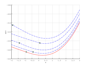
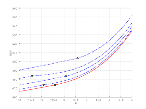
In order to confirm the optimality of the refraction strategy, we plot on the top of Figure 1, for the cases $\beta=-5$ and $\beta=5$, the value function $v_{b^{*}}(x)$ along with suboptimal NPV’s $v_{b}(x)$ for $b\in\{b^{*}-1,b^{*}-0.5,b^{*}+0.5,b^{*}+1\}$. We observe that $v_{b^{*}}$ is indeed minimal (uniformly in $x$) and $b^{*}$ is the sole choice that makes the value function smooth and convex. In addition, the slope at $b^{*}$ of $v_{b^{*}}(x)$ equals $\beta$. This is consistent with our observation that $v_{b^{*}}(x)$ satisfies (4.3).

Figure 1. (Top) Plots of $v_{b}(x)$ for the cases $\beta=-5$ (left) and $\beta=5$ (right). Each panel shows $v_{b^{*}}(x)$ (solid) in comparison to $v_{b}(x)$ (dotted) for $b\in\{b^{*}-1,b^{*}-0.5,b^{*}+0.5,b^{*}+1\}$. The point $(b^{*},v_{b^{*}}(b^{*}))$ is indicated by the square mark on the solid line. Up-pointing and down-pointing triangles show the points $(b,v_{b}(b))$ for $b>b^{*}$ and $b<b^{*}$, respectively. (Bottom) Plots of convergence as $\delta\uparrow\infty$. The left panel shows $b^{*}(\delta)$ for $\delta$ running from $1$ to $100$. The value of $b^{*}(\infty)$ is indicated by the dotted line. On the right panel, the functions $\tilde{v}(x;\delta)$ as in (5.1) are shown as dotted lines for $\delta\in\{1,2,\ldots,20,40,60,80,100\}$. The solid line shows the function $\tilde{v}(x;\infty)$. The square mark indicates the point $(b^{*}(\infty),\tilde{v}(b^{*}(\infty);\infty))$ while the up-pointing triangles show $(b^{*}(\delta),\tilde{v}(b^{*}(\delta);\delta))$.

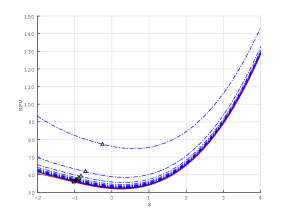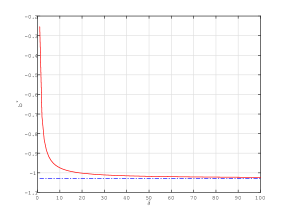
We then analyze the convergence as $\delta\uparrow\infty$. As we have studied in Section 5, we fix the process $Y$ with $\tilde{\gamma}_{Y}=0.5$ and confirm the convergence $\tilde{v}(x;\delta)$ of (5.1) to $\tilde{v}(x;\infty)$ of (5.2). Throughout, we fix $\tilde{\beta}=5$ ($\beta=-5$). At the bottom of Figure 1, we first plot in the left panel the values of $b^{*}(\delta)$ with respect to $\delta$ along with the value of $b^{*}(\infty)$. We see that $b^{*}(\delta)$ is decreasing in $\delta$ and indeed converges to $b^{*}(\infty)$ as $\delta$ gets large. This is consistent with Proposition 5.1. In the right panel, we show the value functions $\tilde{v}(x;\delta)$ as in (5.1) for $\delta\in\{1,2,\ldots,20,40,60,80,100\}$ along with the function $\tilde{v}(x;\infty)$. As has been shown in Theorem 5.1, $\tilde{v}(x;\delta)$ is decreasing in $\delta$ and converges to $\tilde{v}(x;\infty)$.

Appendix A Proof of Lemma 3.1

A.1. Proof of (3.25)

(i) In order to show that the derivative can go into the integral, we shall show that for sufficiently small $-M$,

(A.1) $$\frac{\partial}{\partial x}\int_{-\infty}^{-M}h(y)r_{b}^{(1)}(x,y){\rm d}y=\int_{-\infty}^{-M}h(y)\frac{\partial}{\partial x}r_{b}^{(1)}(x,y){\rm d}y.$$

We first see that, for $\epsilon>0$,

$$r_{b}^{(1)}(x+\epsilon,y)=\mathrm{e}^{\Phi(q)\epsilon}r_{b}^{(1)}(x,y)-W^{(q)}(x+\epsilon-y)+\mathrm{e}^{\Phi(q)\epsilon}W^{(q)}(x-y),\quad y<b,$$

and hence

$$\frac{r_{b}^{(1)}(x+\epsilon,y)-r_{b}^{(1)}(x,y)}{\epsilon}=\frac{\mathrm{e}^{\Phi(q)\epsilon}-1}{\epsilon}r_{b}^{(1)}(x,y)-\mathrm{e}^{\Phi(q)(x+\epsilon-y)}\frac{W_{\Phi(q)}(x+\epsilon-y)-W_{\Phi(q)}(x-y)}{\epsilon}.$$

Here $(\mathrm{e}^{\Phi(q)\epsilon}-1)/\epsilon$ is bounded in $\epsilon>0$ on compacts and $v_{b}^{(1)}(x)=\int_{-\infty}^{\infty}h(y)r_{b}^{(1)}(x,y){\rm d}y$ is well-defined. Hence, for the proof of (A.1), it is sufficient to show that

$$y\mapsto H(y;x,\epsilon):=\left|h(y)\mathrm{e}^{-\Phi(q)y}\frac{W_{\Phi(q)}(x+\epsilon-y)-W_{\Phi(q)}(x-y)}{\epsilon}\right|$$

is bounded in $\epsilon>0$ by a function that is integrable over $(-\infty,-M)$.

First we observe that, by Remark 3.1 (3), $(W_{\Phi(q)}(x+\epsilon-y)-W_{\Phi(q)}(x-y))/\epsilon\leq{\sup}_{0\leq\epsilon^{\prime}\leq\epsilon}W_{\Phi(q)}^{\prime}((x+\epsilon^{\prime}-y)+)$. Moreover, for any $y<0$ and $0<\epsilon^{\prime}<\epsilon$, Remark 3.1 (3) gives

$$\frac{W_{\Phi(q)}^{\prime}((x+\epsilon^{\prime}-y)+)}{W_{\Phi(q)}^{\prime}((x-y)+)}\leq\frac{W_{\Phi(q)}(x+\epsilon^{\prime}-y)}{W_{\Phi(q)}(x-y)}\leq\frac{W_{\Phi(q)}(x+\epsilon-y)}{W_{\Phi(q)}(x-y)}.$$

Fix any $c,k>0$. By (3.5) (and hence $W_{\Phi(q)}(x+k)/W_{\Phi(q)}(x)\xrightarrow{x\uparrow\infty}1$), we can choose sufficiently small $-M<0$, such that for any $y\in(-\infty,-M]$, ${W_{\Phi(q)}(x+k-y)}/{W_{\Phi(q)}(x-y)}\leq 1+c$. Collecting these inequalities, we have a bound $H(y;x,\epsilon)\leq(1+c)\mathrm{e}^{-\Phi(q)y}W^{\prime}_{\Phi(q)}((x-y)+)|h(y)|$ for $0<\epsilon<k$ and $y<-M$. Because (3.10) is finite, we have the claim. Hence (A.1) holds.

(ii) By (i), the derivative can be interchanged over the integral. Hence,

(A.2) $$\begin{split}v_{b}^{(1)\prime}&(x)=-\mathbf{1}_{\{x<b\}}h(x)W^{(q)}(0)+\mathrm{e}^{\Phi(q)(x-b)}\frac{\varphi(q)-\Phi(q)}{\delta}\Big{[}\int_{0}^{\infty}h(y+b)\mathrm{e}^{-\varphi(q)y}{\rm d}y+\frac{\beta\delta}{\varphi(q)}\Big{]}\\ &+\int_{-\infty}^{0}h(y+b)\Big{[}\mathrm{e}^{\Phi(q)(x-b)}(\varphi(q)-\Phi(q))\int_{0}^{\infty}\mathrm{e}^{-\varphi(q)z}W^{(q)\prime}(z-y){\rm d}z-W^{(q)\prime}(x-b-y)\Big{]}{\rm d}y,\end{split}$$

where the first term appears due to the discontinuity of the scale function at zero as in Remark 3.1 (2) for the case of bounded variation.

In order to apply the integration by parts, we first confirm that

(A.3) $$h(y+b)\Big{[}\mathrm{e}^{\Phi(q)(x-b)}(\varphi(q)-\Phi(q))\int_{0}^{\infty}\mathrm{e}^{-\varphi(q)z}W^{(q)}(z-y){\rm d}z-W^{(q)}(x-b-y)\Big{]}\xrightarrow{y\downarrow-\infty}0.$$

Indeed, by (3.18), $\lim_{y\downarrow-\infty}h(y+b)r_{b}^{(1)}(x,y+b)=0$. In addition,

$$r_{b}^{(1)}(x,y+b)-\Big{[}\mathrm{e}^{\Phi(q)(x-b)}(\varphi(q)-\Phi(q))\int_{0}^{\infty}\mathrm{e}^{-\varphi(q)z}W^{(q)}(z-y){\rm d}z-W^{(q)}(x-b-y)\Big{]}$$

$$=\mathrm{e}^{\Phi(q)(x-b)}\frac{\varphi(q)-\Phi(q)}{\Phi(q)}\int_{0}^{\infty}\mathrm{e}^{-\varphi(q)z}\Theta^{(q)}(z-y){\rm d}z=\mathrm{e}^{\Phi(q)(x-b)}\frac{\varphi(q)-\Phi(q)}{q}e^{-\varphi(q)y}\mathbb{E}[\mathrm{e}^{\varphi(q)\underline{X}_{\rm{e}_{q}}}\mathbf{1}_{\{\underline{X}_{\rm{e}_{q}}<y\}}]$$

$$\in\Big{[}0,\mathrm{e}^{\Phi(q)(x-b)}\frac{\varphi(q)-\Phi(q)}{q}\mathbb{P}\{\underline{X}_{\rm{e}_{q}}<y\}\Big{]}.$$

Using identity (3.11) together with Assumption 2.2,

(A.4) $$\mathbb{P}\{\underline{X}_{\rm{e}_{q}}<y\}h(y+b)\xrightarrow{y\downarrow-\infty}0.$$

Hence, (A.3) holds.

Using (3.2), (3.3) and (A.3), together with the following identity

(A.5) $$\int_{0}^{\infty}\mathrm{e}^{-\varphi(q)z}W^{(q)}(z){\rm d}z=(\psi(\varphi(q))-q)^{-1}=(\varphi(q)\delta)^{-1},$$

integration by parts yields

$$v_{b}^{(1)\prime}(x) =\mathrm{e}^{\Phi(q)(x-b)}\frac{\varphi(q)-\Phi(q)}{\delta\varphi(q)}\Big{[}\int_{0}^{\infty}\mathrm{e}^{-\varphi(q)y}h^{\prime}(y+b){\rm d}y+{\beta\delta}\Big{]}+h(b)W^{(q)}(x-b)$$

$$+\int_{-\infty}^{0}h^{\prime}(y+b)\Big{[}\mathrm{e}^{\Phi(q)(x-b)}(\varphi(q)-\Phi(q))\int_{0}^{\infty}\mathrm{e}^{-\varphi(q)z}W^{(q)}(z-y){\rm d}z-W^{(q)}(x-b-y)\Big{]}{\rm d}y.$$

Taking the difference between this and $\int_{-\infty}^{\infty}h^{\prime}(y)r_{b}^{(1)}(x,y){\rm d}y$, we have the result.

A.2. Proof of (3.26)

In view of (3.17), let us decompose $v_{b}^{(2)}(x)=v_{b}^{(2,1)}(x)+\delta v_{b}^{(2,2)}(x)$ where

$$\begin{split}v_{b}^{(2,1)}(x)&:=\int_{0}^{\infty}(h(y+b)+\beta\delta)\Big{\{}\mathrm{e}^{-\varphi(q)y}M(x;b)-\mathbb{W}^{(q)}(x-b-y)\Big{\}}{\rm d}y,\\ v_{b}^{(2,2)}(x)&:=\int_{-\infty}^{0}h(y+b)\Big{\{}M(x;b)\int_{0}^{\infty}\mathrm{e}^{-\varphi(q)z}W^{(q)\prime}(z-y){\rm d}z-\int_{b}^{x}\mathbb{W}^{(q)}(x-z)W^{(q)\prime}(z-b-y){\rm d}z\Big{\}}{\rm d}y.\end{split}$$

For the function $v_{b}^{(2,1)}$, integration by parts gives

$$v_{b}^{(2,1)}(x)=(h(b)+\beta\delta)\Big{\{}\frac{M(x;b)}{\varphi(q)}-\int_{0}^{x-b}\mathbb{W}^{(q)}(z){\rm d}z\Big{\}}+\int_{0}^{\infty}h^{\prime}(y+b)\Big{\{}\frac{M(x;b)}{\varphi(q)}\mathrm{e}^{-\varphi(q)y}-\int_{0}^{x-b-y}\mathbb{W}^{(q)}(z){\rm d}z\Big{\}}{\rm d}y.$$

Differentiating this and noting that

(A.6) $$M^{\prime}(x;b) =(\varphi(q)-\Phi(q))\mathbb{W}^{(q)}(x-b)+\Phi(q)M(x;b),$$

we have

(A.7) $$v_{b}^{(2,1)\prime}(x)=\frac{\Phi(q)}{\varphi(q)}(h(b)+\beta\delta)\Big{\{}{-\mathbb{W}^{(q)}(x-b)+M(x;b)}\Big{\}}\\ +\int_{0}^{\infty}h^{\prime}(y+b)\Big{\{}\frac{(\varphi(q)-\Phi(q))\mathbb{W}^{(q)}(x-b)+\Phi(q)M(x;b)}{\varphi(q)}\mathrm{e}^{-\varphi(q)y}-\mathbb{W}^{(q)}(x-b-y)\Big{\}}{\rm d}y.$$

In order to deal with the function $v_{b}^{(2,2)}$, we shall first show the limit

(A.8) $$\lim_{y\downarrow-\infty}h(y+b)N(y;x,b)=0,$$

where we define

$$N(y;x,b):=M(x;b)\int_{0}^{\infty}\mathrm{e}^{-\varphi(q)z}W^{(q)}(z-y){\rm d}z-\int_{b}^{x}\mathbb{W}^{(q)}(x-z)W^{(q)}(z-b-y){\rm d}z,$$

so as to apply the integration by parts.

First, because $v^{(2)}_{b}$ is well defined and finite by (3.19), $\lim_{y\downarrow-\infty}h(y+b)r_{b}^{(2)}(x,y+b)=0$. In addition,

$$\delta^{-1}r_{b}^{(2)}(x,y+b)-\Phi(q)N(y;x,b)=M(x;b)\int_{0}^{\infty}\mathrm{e}^{-\varphi(q)z}\Theta^{(q)}(z-y){\rm d}z-\int_{b}^{x}\mathbb{W}^{(q)}(x-z)\Theta^{(q)}(z-b-y){\rm d}z,$$

whose absolute value is bounded by

$$M(x;b)\int_{0}^{\infty}\mathrm{e}^{-\varphi(q)z}\Theta^{(q)}(z-y){\rm d}z+\int_{b}^{x}\mathbb{W}^{(q)}(x-z)\Theta^{(q)}(z-b-y){\rm d}z$$

$$\leq M(x;b)\int_{0}^{\infty}\mathrm{e}^{-\varphi(q)z}\Theta^{(q)}(z-y){\rm d}z+\mathbb{W}_{\varphi(q)}(x-b)\int_{0}^{\infty}\mathrm{e}^{\varphi(q)(x-z-b)}\Theta^{(q)}(z-y){\rm d}z$$

$$=\Big{(}M(x;b)e^{-\varphi(q)y}\mathbb{E}[\mathrm{e}^{\varphi(q)\underline{X}_{\rm{e}_{q}}}\mathbf{1}_{\{\underline{X}_{\rm{e}_{q}}<y\}}]+\mathbb{W}_{\varphi(q)}(x-b)\mathrm{e}^{-\varphi(q)(x-b)}e^{-\varphi(q)y}\mathbb{E}[\mathrm{e}^{\varphi(q)\underline{X}_{\rm{e}_{q}}}\mathbf{1}_{\{\underline{X}_{\rm{e}_{q}}<y\}}]\Big{)}\frac{\Phi(q)}{q}$$

$$\leq[M(x;b)+\mathbb{W}_{\varphi(q)}(x-b)\mathrm{e}^{-\varphi(q)(x-b)}]\mathbb{P}\{\underline{X}_{\rm{e}_{q}}<y\}\frac{\Phi(q)}{q},$$

where $\mathbb{W}_{\varphi(q)}(z):=\mathrm{e}^{-\varphi(q)z}\mathbb{W}^{(q)}(z)$. This together with (A.4) shows the limit (A.8).

Now, integration by parts followed by Fubini’s theorem, together with the identities (A.5) and $\int_{b}^{x}\mathbb{W}^{(q)}(x-z)W^{(q)}(z-b){\rm d}z=\delta^{-1}(\int_{0}^{x-b}\mathbb{W}^{(q)}(z){\rm d}z-\int_{0}^{x-b}{W}^{(q)}(z){\rm d}z)$, gives

$$v_{b}^{(2,2)}(x) =\frac{h(b)}{\delta}\Big{\{}-\frac{M(x;b)}{\varphi(q)}+\int_{0}^{x-b}\mathbb{W}^{(q)}(z){\rm d}z-\int_{0}^{x-b}{W}^{(q)}(z){\rm d}z\Big{\}}+\int_{b}^{x}\mathbb{W}^{(q)}(x-z)A(z;b){\rm d}z.$$

Here we define

$$A(z;b):=\int_{-\infty}^{0}h^{\prime}(y+b)\Big{\{}(\varphi(q)-\Phi(q))\mathrm{e}^{-\Phi(q)(b-z)}\int_{0}^{\infty}\mathrm{e}^{-\varphi(q)w}W^{(q)}(w-y){\rm d}w-W^{(q)}(z-y-b)\Big{\}}{\rm d}y,$$

which is finite for all $z\in[b,x]$. Indeed, we have $A(z;b)=e^{-\Phi(q)(z-x)}A(x;b)+\int_{-\infty}^{0}h^{\prime}(y+b)(e^{-\Phi(q)(z-x)}W^{(q)}(x-y-b)-W^{(q)}(z-y-b)){\rm d}y$ where the integral part is finite by similar arguments as in Remark 3.3; if it is infinity, it contradicts with that $v_{b}^{(2,2)}$ is finite.

Hence, taking a derivative and by (A.6),

$$v_{b}^{(2,2)\prime}(x) =\frac{h(b)}{\delta}\Big{\{}-\frac{M^{\prime}(x;b)}{\varphi(q)}+\mathbb{W}^{(q)}(x-b)-W^{(q)}(x-b)\Big{\}}+\int_{-\infty}^{0}h^{\prime}(y+b)B(y,x,b){\rm d}y$$

$$=\frac{h(b)}{\delta}\Big{\{}\frac{\Phi(q)}{\varphi(q)}\Big{(}\mathbb{W}^{(q)}(x-b)-M(x;b)\Big{)}-W^{(q)}(x-b)\Big{\}}+\int_{-\infty}^{0}h^{\prime}(y+b)B(y,x,b){\rm d}y$$

with

$$B(y,x,b) :=\mathbb{W}^{(q)}(0)\Big{\{}(\varphi(q)-\Phi(q))\mathrm{e}^{-\Phi(q)(b-x)}\int_{0}^{\infty}\mathrm{e}^{-\varphi(q)w}W^{(q)}(w-y){\rm d}w-W^{(q)}(x-y-b)\Big{\}}$$

$$+\int_{b}^{x}\mathbb{W}^{(q)\prime}(x-z)\Big{\{}(\varphi(q)-\Phi(q))\mathrm{e}^{-\Phi(q)(b-z)}\int_{0}^{\infty}\mathrm{e}^{-\varphi(q)w}W^{(q)}(w-y){\rm d}w-W^{(q)}(z-y-b)\Big{\}}{\rm d}z.$$

By (3.24) and integration by parts, we can write

$$B(y,x,b) =\frac{(\varphi(q)-\Phi(q))\mathbb{W}^{(q)}(x-b)+\Phi(q)M(x;b)}{\varphi(q)}\Big{(}\int_{0}^{\infty}\mathrm{e}^{-\varphi(q)z}W^{(q)\prime}(z-y){\rm d}z+W^{(q)}(-y)\Big{)}$$

$$-\mathbb{W}^{(q)}(x-b)W^{(q)}(-y)-\int_{b}^{x}\mathbb{W}^{(q)}(x-z)W^{(q)\prime}(z-y-b){\rm d}z.$$

From this and (A.7), the expression $\int_{-\infty}^{\infty}h^{\prime}(y)r_{b}^{(2)}(x,y){\rm d}y-(v_{b}^{(2,1)\prime}(x)+\delta v_{b}^{(2,2)\prime}(x))$ gives the result after some calculations.

Appendix B Proof of Lemma 4.2

In view of the expression (3.30), $v_{b^{*}}^{\prime}$ is continuous for all $x\in\mathbb{R}$. Hence, it remains to show that $v_{b^{*}}^{\prime}$ is continuously differentiable for the case of unbounded variation.

By (3.12) and (3.30), we can write $v_{b^{*}}^{\prime}(x)=w^{(1)}(x)+w^{(2)}(x)\mathbf{1}_{\{x>b^{*}\}}$ where

$$w^{(1)}(x) :=\frac{\varphi(q)-\Phi(q)}{\delta\Phi(q)}\int_{0}^{\infty}h^{\prime}(y+b^{*})\mathrm{e}^{\Phi(q)(x-b^{*})-\varphi(q)y}{\rm d}y$$

$$+\int_{-\infty}^{0}h^{\prime}(y+b^{*})\Big{[}\mathrm{e}^{\Phi(q)(x-b^{*})}\frac{\varphi(q)-\Phi(q)}{\Phi(q)}\int_{0}^{\infty}\mathrm{e}^{-\varphi(q)z}W^{(q)\prime}(z-y){\rm d}z-W^{(q)}(x-b^{*}-y)\Big{]}{\rm d}y,$$

$$w^{(2)}(x) :=\int_{0}^{\infty}h^{\prime}(y+b^{*})\Big{\{}\mathrm{e}^{-\varphi(q)y}M(x;b^{*})-\mathbb{W}^{(q)}(x-b^{*}-y)\Big{\}}{\rm d}y$$

$$+\delta\int_{-\infty}^{0}h^{\prime}(y+b^{*})\Big{\{}M(x;b^{*})\int_{0}^{\infty}\mathrm{e}^{-\varphi(q)z}W^{(q)\prime}(z-y){\rm d}z-\int_{b^{*}}^{x}\mathbb{W}^{(q)}(x-z)W^{(q)\prime}(z-b^{*}-y){\rm d}z\Big{\}}{\rm d}y.$$

Notice that (A.1) holds when $h$ is replaced with $h^{\prime}$ (by Assumption 2.2). Hence, similarly to (A.2) (noting that $W^{(q)}(0)=0$ for the case of unbounded variation),

$$w^{(1)\prime}(x) =\frac{\varphi(q)-\Phi(q)}{\delta}\int_{0}^{\infty}h^{\prime}(y+b^{*})\mathrm{e}^{\Phi(q)(x-b^{*})-\varphi(q)y}{\rm d}y$$

$$+\int_{-\infty}^{0}h^{\prime}(y+b^{*})\Big{[}\mathrm{e}^{\Phi(q)(x-b^{*})}(\varphi(q)-\Phi(q))\int_{0}^{\infty}\mathrm{e}^{-\varphi(q)z}W^{(q)\prime}(z-y){\rm d}z-W^{(q)\prime}(x-b^{*}-y)\Big{]}{\rm d}y.$$

In addition, with the help of Fubini’s theorem and noticing that $W^{(q)}(0)=0$,

$$w^{(2)\prime}(x) =\int_{b^{*}}^{\infty}h^{\prime}(y)\Big{\{}\mathrm{e}^{-\varphi(q)(y-b^{*})}M^{\prime}(x;b^{*})-\mathbb{W}^{(q)\prime}(x-y)\Big{\}}{\rm d}y$$

$$+\delta\int_{b^{*}}^{x}\mathbb{W}^{(q)\prime}(x-z)\int_{-\infty}^{0}h^{\prime}(y+b^{*})\Big{\{}(\varphi(q)-\Phi(q))\mathrm{e}^{-\Phi(q)(b^{*}-z)}\int_{0}^{\infty}\mathrm{e}^{-\varphi(q)w}W^{(q)\prime}(w-y){\rm d}w$$

$$\qquad-W^{(q)\prime}(z-b^{*}-y)\Big{\}}{\rm d}y{\rm d}z.$$

The continuity of $w^{(1)\prime}$ and $w^{(2)\prime}$ are clear for $x\neq b^{*}$. We have

$$\int_{-\infty}^{0}h^{\prime}(y+b^{*})\Big{\{}(\varphi(q)-\Phi(q))\mathrm{e}^{-\Phi(q)(b^{*}-z)}\int_{0}^{\infty}\mathrm{e}^{-\varphi(q)w}W^{(q)\prime}(w-y){\rm d}w-W^{(q)\prime}(z-b^{*}-y)\Big{\}}{\rm d}y$$

$$=\int_{-\infty}^{0}h^{\prime}(y+b^{*})\Big{\{}\Phi(q)r_{b}^{(1)}(z-b^{*},y)-\Theta^{(q)}(z-b^{*}-y)\Big{\}}{\rm d}y.$$

By (3.7) and Remark 3.3, this is finite for $z\in[b^{*},x]$. Hence, $\lim_{x\downarrow b^{*}}w^{(2)\prime}(x)=0$.

References

- [1] S. Asmussen, F. Avram, and M. R. Pistorius. Russian and American put options under exponential phase-type Lévy models. Stochastic Process. Appl., 109(1):79–111, 2004.
- [2] F. Avram, Z. Palmowski, and M. R. Pistorius. On the optimal dividend problem for a spectrally negative Lévy process. Ann. Appl. Probab., 17(1):156–180, 2007.
- [3] S. Baccarin. Optimal impulse control for cash management with quadratic holding-penalty costs. Decisions in Economics and Finance, 25(1):19–32, 2002.
- [4] E. J. Baurdoux and K. Yamazaki. Optimality of doubly reflected Lévy processes in singular control. Stochastic Process. Appl., 125(7):2727–2751, 2015.
- [5] E. Bayraktar, A. E. Kyprianou, and K. Yamazaki. On optimal dividends in the dual model. Astin Bull., 43(3):359–372, 2013.
- [6] L. Benkherouf and A. Bensoussan. Optimality of an policy with compound Poisson and diffusion demands: a quasi-variational inequalities approach. SIAM J. Control Optim., 48(2):756–762, 2009.
- [7] A. Bensoussan, R. H. Liu, and S. P. Sethi. Optimality of an policy with compound Poisson and diffusion demands: a quasi-variational inequalities approach. SIAM J. Control Optim., 44(5):1650–1676, 2005.
- [8] T. Chan, A. E. Kyprianou, and M. Savov. Smoothness of scale functions for spectrally negative Lévy processes. Probab. Theory Relat. Fields, 150:691–708, 2011.
- [9] G. M. Constantinides and S. F. Richard. Existence of optimal simple policies for discounted-cost inventory and cash management in continuous time. Oper. Res., 26(4):620–636, 1978.
- [10] M. Egami and K. Yamazaki. Phase-type fitting of scale functions for spectrally negative Lévy processes. J. Comput. Appl. Math., 264:1–22, 2014.
- [11] D. Hernández-Hernández and K. Yamazaki. Games of singular control and stopping driven by spectrally one-sided Lévy processes. Stochastic Process. Appl., 125:1–38, 2015.
- [12] M. Jeanblanc-Picqué. Impulse control method and exchange rate. Mathematical Finance, 3(2):161–177, 1993.
- [13] A. Kuznetsov, A. Kyprianou, and V. Rivero. The theory of scale functions for spectrally negative Lévy processes. Springer Lecture Notes in Mathematics, 2061:97–186, 2013.
- [14] A. E. Kyprianou. Fluctuations of Lévy processes with applications. Universitext. Springer-Verlag, Berlin, second edition, 2014.
- [15] A. E. Kyprianou and R. L. Loeffen. Refracted Lévy processes. Ann. Inst. H. Poincaré, 46(1):24–44, 2010.
- [16] A. E. Kyprianou, R. L. Loeffen, and J. Pérez. Optimal control with absolutely continuous strategies for spectrally negative Lévy processes. J. Appl. Probab., 49:150–166, 2012.
- [17] R. L. Loeffen. On optimality of the barrier strategy in de Finetti’s dividend problem for spectrally negative Lévy processes. Ann. Appl. Probab., 18(5):1669–1680, 2008.
- [18] G. Mundaca and B. Øksendal. Optimal stochastic intervention control with application to the exchange rate. Journal of Mathematical Economics, 29(2):225–243, 1998.
- [19] P. E. Protter. Stochastic integration and differential equations, volume 21 of Stochastic Modelling and Applied Probability. Springer-Verlag, Berlin, 2005. Second edition. Version 2.1, Corrected third printing.
- [20] A. Sulem. A solvable one-dimensional model of a diffusion inventory system. Math. Oper. Res., 11(1):125–133, 1986.
- [21] K. Yamazaki. Inventory control for spectrally positive Lévy demand processes. Math. Oper. Res., forthcoming.