On an adaptive regularization for ill-posed nonlinear systems and its trust-region implementation

Abstract

In this paper we address the stable numerical solution of nonlinear ill-posed systems by a trust-region method. We show that an appropriate choice of the trust-region radius gives rise to a procedure that has the potential to approach a solution of the unperturbed system. This regularizing property is shown theoretically and validated numerically.

Keywords: Ill-posed systems of nonlinear equations, regularization, nonlinear stepsize control, trust-region methods.

1 Introduction

Nonlinear systems modeling inverse problems are typically ill-posed, in the sense that their solutions do not depend continuously on the data and their data are affected by noise [4, 14, 22]. In this work we focus on the stable approximation of a solution of these problems. Procedures in the classes of Levenberg-Marquardt and trust-region methods are discussed, and a suitable version of trust-region algorithm is shown to have regularizing properties both theoretically and numerically. The underlying motivation for our study is twofold: most of the practical methods in literature have been designed for well-posed systems, see e.g., [3, 19], and thus are unsuited in the context of inverse problems; adaptation of existing procedures for handling ill-posed problems, carried out in the seminal papers [8, 10, 11, 13, 21, 23], deserves further theoretical and numerical insights.

Let

$$F(x)=y,$$ (1.1)

with $F:\mathbb{R}^{n}\rightarrow\mathbb{R}^{n}$ continuously differentiable, be obtained from the discretization of a problem modeling an inverse problem. It is realistic to have noisy data $y^{\delta}$ at disposal, satisfying

$$||y-y^{\delta}||_{2}\leq\delta,$$ (1.2)

for some positive $\delta$. Thus, in practice it is necessary to solve a problem of the form

$$F(x)=y^{\delta},$$ (1.3)

and, due to ill-posedeness, possible solutions may be arbitrarily far from those of the original problem.

In [10, 11], Hanke supposed that an initial guess, close enough to some solution $x^{\dagger}$ of (1.1), is available. Then, he proposed a regularizing Levenberg-Marquardt procedure which is able to compute a stable approximation $x_{k_{*}}^{\delta}$ to $x^{\dagger}$ or to some other solution of the unperturbed problem (1.1) close to $x^{\dagger}$. This task is achieved through a nonlinear stepsize control in the Levenberg-Marquardt procedure and the discrepancy principle as the stopping criterion, so that the iterative process is stopped at the iteration $k_{*}$ satisfying

$$\|y^{\delta}-F(x_{k_{*}}^{\delta})\|_{2}\leq\tau\delta<\|y^{\delta}-F(x_{k}^{\delta})\|_{2},\;\;\;0\leq k<k_{*},$$ (1.4)

with $\tau>1$ appropriately chosen [18]. Remarkably $x_{k_{*}}^{\delta}$ converges to a solution of (1.1) as $\delta$ tends to zero.

Further regularizing iterative methods have been proposed, including first-order methods and Newton-type methods. Analogously to the Levenberg-Marquardt procedure proposed by Hanke, instead of promoting convergence to a solution of (1.3), they form approximations of increasing accuracy to some solution of the unperturbed problem (1.1) until the discrepancy principle (1.4) is met. We refer to [4, 14] for the description and analysis of such methods.

The above mentioned regularizing Levenberg-Marquardt method belongs to the unifying framework of nonlinear stepsize control algorithms for unconstrained optimization developed by Toint [20] and including trust-region methods [3]. Therefore, elaborating on original ideas by Hanke, we introduce and analyze a regularizing variant of the trust-region method. The main feature of our variant is the rule for selecting the trust-region radius which guarantees two properties. First, it guarantees the same regularizing properties as the method by Hanke. Second, as for standard trust-region procedure, it enforces a monotonic decrease of the value of the function

$$\Phi(x)=\frac{1}{2}\|y^{\delta}-F(x)\|_{2}^{2},$$ (1.5)

at the iterates $x_{k}^{\delta}$. Convergence properties are enhanced with respect to the regularizing Levenberg-Marquardt procedure in the following respects. With exact data, if there exists an accumulation point of the iterates which solves (1.1), then any accumulation point of the sequence solves (1.1). With noisy data, the methods have the potential to satisfy the discrepancy principle (1.4). As for standard trust-region methods, these properties can be enhanced independently of the closeness of the initial guess to a solution of (1.1).

Our contribution covers theoretical and practical aspects of the method proposed. From a theoretical point of view, we propose the use of a trust-region radius converging to zero as $\delta$ tends to zero. Trust-region methods with this distinguishing feature have been proposed in several papers, see [5, 6, 7, 25], but none of such works was either devised for ill-posed problems or applied to them; thus, our study offers new insights on the potential of this choice for the trust-region radius. Moreover, we have made a first attempt toward global convergent methods for ill-posed problems; to our knowledge, this topic has been considered only in a multilevel approach proposed by Kaltenbacher [13]. Finally, local convergence analysis has been carried out without the assumption (commonly made in literature) on the boundness of the inverse of the Jacobian $J$ of $F$, since it may not be fulfilled in the situation of ill-posedeness. Taking into account that the standard convergence analysis of trust-region methods always requires the invertibility of $J$, our results represent a progress in the theoretical investigation of convergence. Concerning numerical aspects, we discuss an implementation of the regularizing trust-region method, and test its ability to approximate a solution of (1.1) in presence of noise. Comparison with a standard trust-region scheme highlights the impact of the proposed trust-region radius choice on regularization.

The paper is organized as follows. In §2 we describe the main features of the regularizing Levenberg-Marquardt method proposed by Hanke. In §3 we introduce our regularizing version of the trust-region methods and in §4 we study the local convergence properties. A comparative numerical analysis of all the procedures studied is done in §5.

Notations. We indicate the iterates of the procedures analyzed as $x_{k}^{\delta}$; if the data are exact, $x_{k}$ may be used in alternative to $x_{k}^{\delta}$. By $x_{0}^{\delta}=x_{0}$ we denote an initial guess which may incorporate a-priori knowledge of an exact solution. The symbol $\|\cdot\|$ indicates the Euclidean norm. The Jacobian matrix of $F$ is denoted as $J$.

2 Regularizing Levenberg-Marquardt method for ill-posed problems

We describe the regularizing version of the Levenberg-Marquardt method proposed in [10] for solving (1.3), and analyze some issues for its practical implementation.

At $k$-th iteration of the Levenberg-Marquardt, given $x_{k}^{\delta}\in\mathbb{R}^{n}$ and $\lambda_{k}>0$, let

$$m_{k}^{\mathrm{LM}}(p)=\frac{1}{2}\|F(x_{k}^{\delta})-y^{\delta}+J(x_{k}^{\delta})p\|^{2}+\frac{1}{2}\lambda_{k}\|p\|^{2},$$ (2.6)

be a quadratic model around $x_{k}^{\delta}$ for the function $\Phi$ in (1.5), see [15, 16]. The step $p_{k}$ taken minimizes $m_{k}^{\mathrm{LM}}$, and $x_{k+1}^{\delta}=x_{k}^{\delta}+p_{k}$. We observe that, if $p(\lambda)$ is the solution of

$$(B_{k}+\lambda I)p(\lambda)=-g_{k},$$ (2.7)

with $B_{k}=J(x_{k}^{\delta})^{T}J(x_{k}^{\delta})$ and $g_{k}=J(x_{k}^{\delta})^{T}(F(x_{k}^{\delta})-y^{\delta})$, then $p_{k}=p(\lambda_{k})$.

If problem (1.3) is ill-posed, and the scalars $\lambda_{k}$ are limited to promote convergence of procedure, see [16], then the solution of (1.1) may be significantly misinterpreted [9, 14, 22]. The regularizing Levenberg-Marquardt method [10] attempts to approximate solutions of (1.1) by choosing $\lambda_{k}$ as the solution $\lambda_{k}^{q}$ of the nonlinear scalar equation

$$\|F(x_{k}^{\delta})-y^{\delta}+J(x_{k}^{\delta})p(\lambda)\|=q\|F(x_{k}^{\delta})-y^{\delta}\|,$$ (2.8)

for some fixed $q\in(0,1)$. Under suitable assumptions discussed below, $\lambda_{k}^{q}$ is uniquely determined from (2.8).

As for (2.8), it is useful to establish relations between $\lambda$, $\|p(\lambda)\|$ and $\|F(x_{k}^{\delta})-y^{\delta}+J(x_{k}^{\delta})p(\lambda)\|$.

Lemma 1.

[1, Lemma 4.2] Suppose $\|g_{k}\|\neq 0$ and let $p(\lambda)$ be the minimum norm solution of (2.7) with $\lambda\geq 0$. Suppose furthermore that $J(x_{k}^{\delta})$ is of rank $\ell$ and its singular-value decomposition is given by $U_{k}\Sigma_{k}V_{k}^{T}$ where $\Sigma_{k}$ is the diagonal matrix with entries $\varsigma_{1},\ldots,\varsigma_{n}$ on the diagonal. Then, denoting $r=(r_{1},r_{2},\dots,r_{n})^{T}=U_{k}^{T}(F(x_{k}^{\delta})-y^{\delta})$, we have that

$$\|p(\lambda)\|^{2}=\sum_{i=1}^{\ell}\frac{\varsigma_{i}^{2}r_{i}^{2}}{(\varsigma_{i}^{2}+\lambda)^{2}},$$ (2.9)

$$\|F(x_{k}^{\delta})-y^{\delta}+J(x_{k}^{\delta})p(\lambda)\|^{2}=\sum_{i=1}^{\ell}\frac{\lambda^{2}r_{i}^{2}}{(\varsigma_{i}^{2}+\lambda)^{2}}+\sum_{i=\ell+1}^{n}r_{i}^{2}.$$ (2.10)

Using this result, the solution of (2.8) is characterized as follows.

Lemma 2.

Suppose $\|g_{k}\|\neq 0$. Let $p(\lambda)$ be the minimum norm solution of (2.7) with $\lambda\geq 0$, $\mathcal{R}(J(x_{k}^{\delta}))^{\bot}$ be the orthogonal complement of the range $\mathcal{R}(J(x_{k}^{\delta}))$ of $J(x_{k}^{\delta})$, and $P_{k}^{\delta}$ be the orthogonal projector onto $\mathcal{R}(J(x_{k}^{\delta}))^{\bot}$. Then

(i) Equation (2.8) is not solvable if $\|P_{k}^{\delta}(F(x_{k}^{\delta})-y^{\delta})\|>q\|F(x_{k}^{\delta})-y^{\delta}\|$.

(ii) If

$$\|F(x_{k}^{\delta})-y^{\delta}+J(x_{k}^{\delta})(x^{\dagger}-x_{k}^{\delta})\|\leq\frac{q}{\theta_{k}}\|F(x_{k}^{\delta})-y^{\delta}\|,$$ (2.11)

for some $\theta_{k}>1$, then equation (2.8) has a unique solution $\lambda_{k}^{q}$ such that

$$\lambda_{k}^{q}\in\left(0,\frac{q}{1-q}\|B_{k}\|\right].$$ (2.12)

Proof.

$(i)$ Equation (2.10) implies

$$\lim_{\lambda\rightarrow 0}\|F(x_{k}^{\delta})-y^{\delta}+J(x_{k}^{\delta})p(\lambda)\|=\|P_{k}^{\delta}(F(x_{k}^{\delta})-y^{\delta})\|,$$

$$\lim_{\lambda\rightarrow\infty}\|F(x_{k}^{\delta})-y^{\delta}+J(x_{k}^{\delta})p(\lambda)\|=\|F(x_{k}^{\delta})-y^{\delta}\|.$$

Thus, since $\|F(x_{k}^{\delta})-y^{\delta}+J(x_{k}^{\delta})p(\lambda)\|$ is monotonically increasing as a function of $\lambda$, we conclude that (2.8) does not admit solution if $\|P_{k}^{\delta}(F(x_{k}^{\delta})-y^{\delta})\|>q\|F(x_{k}^{\delta})-y^{\delta}\|$.

$(ii)$ Trivially $\|P_{k}^{\delta}(F(x_{k}^{\delta})-y^{\delta})\|\leq\|F(x_{k}^{\delta})-y^{\delta}+J(x_{k}^{\delta})(x-x_{k}^{\delta})\|$, for any $x$. Hence, for the monotonicity of $\|F(x_{k}^{\delta})-y^{\delta}+J(x_{k}^{\delta})p(\lambda)\|$, if (2.11) holds, then equation (2.8) admits a solution which is positive and unique. Finally,

$$F(x_{k}^{\delta})-y^{\delta}+J(x_{k}^{\delta})p(\lambda)=\lambda(J(x_{k}^{\delta})J(x_{k}^{\delta})^{T}+\lambda I)^{-1}(F(x_{k}^{\delta})-y^{\delta}),$$

see e.g., [10, Proposition 2.1], and by (2.8)

$$q\|F(x_{k}^{\delta})-y^{\delta}\| = \lambda_{k}^{q}\|(J(x_{k}^{\delta})J(x_{k}^{\delta})^{T}+\lambda_{k}^{q}I)^{-1}(F(x_{k}^{\delta})-y^{\delta})\|$$

$$\geq \frac{\lambda_{k}^{q}}{\|J(x_{k}^{\delta})\|^{2}+\lambda_{k}^{q}}\|F(x_{k}^{\delta})-y^{\delta}\|,$$

which yields (2.12). ∎

In [10], the analysis of resulting Levenberg-Marquardt method was made under the subsequent assumptions on the solvability of the problem (1.1), the Taylor remainder of $F$, and the vicinity of the initial guess $x_{0}$ to some solution $x^{\dagger}$ of (1.1).

Assumption 2.1.

Given an initial guess $x_{0}$, there exist positive $\rho$ and $c$ such that system (1.1) is solvable in $B_{\rho}(x_{0})$, and

$$\quad\|F(x)-F(\tilde{x})-J(x)(x-\tilde{x})\|\leq c\|x-\tilde{x}\|\,\|F(x)-F(\tilde{x})\|,\;\;\;x,\tilde{x}\in B_{2\rho}(x_{0}).$$ (2.13)

Assumption 2.2.

Let $x_{0}$, $c$ and $\rho$ as in Assumption 2.1, $x^{\dagger}$ be a solution of (1.1) and $x_{0}$ satisfy

$$\|x_{0}-x^{\dagger}\| < \min\left\{\frac{q}{c},\rho\right\},\hskip 43.0pt\mbox{if}\;\;\;\;\delta=0,$$ (2.14)

$$\|x_{0}-x^{\dagger}\| < \min\left\{\frac{q\tau-1}{c(1+\tau)},\rho\right\},\;\;\;\;\mbox{if}\;\;\;\;\delta>0$$ (2.15)

where $\tau>1/q$.

From Assumption 2.1 it follows that inequality (2.11) is satisfied for any $x_{k}^{\delta}$ belonging to $B_{2\rho}(x_{0})$ and consequently there exists a solution to (2.8), see [10, Theorems 2.2, 2.3].

Under Assumptions 2.1 and 2.2, the approximations $x_{k^{*}}^{\delta}$ generated by the Levenberg-Marquardt method satisfy (1.4) and converge to a solution of (1.1) as $\delta$ tends to zero.

Theorem 3.

Let Assumptions 2.1 and 2.2 hold and $x_{k}^{\delta}$ be the Levenberg-Marquardt iterates determined by using (2.8). For noisy data, suppose $k<k_{*}$ where $k_{*}$ is defined in (1.4). Then, any iterate $x_{k}^{\delta}$ belongs to $B_{2\rho}(x_{0})$. With exact data, the sequence $\{x_{k}\}$ converges to a solution of (1.1). With noisy data, the stopping criterion (1.4) is satisfied after a finite number $k_{*}$ of iterations and $\{x_{k^{*}}^{\delta}\}$ converges to a solution of (1.1) as $\delta$ goes to zero.

Proof.

See [10], Theorem 2.2 and Theorem 2.3. ∎

Let us focus on a specific issue concerning the implementation of the method which, to our knowledge, has not been addressed either in [10] or in related papers. The numerical solution of (2.8) requires the application of a root-finder method and Newton method is the most efficient procedure, though in general it requires the knowledge of an accurate approximation to the solution. On the other hand, nonlinear equations which are monotone and convex (or concave) on some interval containing the root are particularly suited to an application of Newton method, see e.g. [12, Theorem 4.8]. Equation (2.8) does not have such properties but it can be replaced by an equivalent equation with strictly decreasing and concave function in $[\lambda_{k}^{q},\infty)$; thus, Newton method applied to the reformulated equation converges globally to $\lambda_{k}^{q}$ whenever the initial guess overestimates such a root.

Lemma 4.

Suppose $\|F(x_{k}^{\delta})-y^{\delta}\|\neq 0$, and that (2.8) has positive solution $\lambda_{k}^{q}$. Let

$$\psi(\lambda)=\frac{\lambda}{\|F(x_{k}^{\delta})-y^{\delta}+J(x_{k}^{\delta})p(\lambda)\|}-\frac{\lambda}{q\|F(x_{k}^{\delta})-y^{\delta}\|}=0.$$ (2.16)

Then, Newton method applied to (2.16) converges monotonically and globally to the root $\lambda_{k}^{q}$ of (2.8) for any initial guess in the interval $[\lambda_{k}^{q},\infty)$.

Proof.

Trivially, solving (2.8) is equivalent to finding the positive root of the equation (2.16). We now show that $\psi(\lambda)$ is strictly decreasing in $[\lambda_{k}^{q},\infty)$ and concave on $(0,\infty)$. By (2.10),

$$\frac{\lambda}{\|F(x_{k}^{\delta})-y^{\delta}+J(x_{k}^{\delta})p(\lambda)\|}=\left(\,\sqrt{\sum_{i=1}^{l}\left(\frac{r_{i}}{\zeta_{i}^{2}+\lambda}\right)^{2}+\sum_{i=l+1}^{n}\left(\frac{r_{i}}{\lambda}\right)^{2}}\,\right)^{-1},$$ (2.17)

and this function is concave on $(0,\infty)$, cfr. [2, Lemma 2.1]. Thus, $\psi$ is concave on $(0,\infty)$ and trivially $\psi^{\prime}(\lambda)$ is strictly decreasing.

Now we show that $\psi^{\prime}(\lambda_{k}^{q})$ is negative; thus, using the monotonicity of $\psi^{\prime}(\lambda)$, we get that $\psi(\lambda)$ is strictly decreasing in $[\lambda_{k}^{q},\infty)$. Differentiation of $\psi(\lambda)$ and (2.8) give

$$\psi^{\prime}(\lambda_{k}^{q}) = \frac{(\lambda_{k}^{q})^{3}}{\|F(x_{k}^{\delta})-y^{\delta}+J(x_{k}^{\delta})p(\lambda_{k}^{q})\|^{3}}\left(\sum_{i=1}^{l}\frac{r_{i}^{2}}{(\zeta_{i}^{2}+\lambda_{k}^{q})^{3}}+\sum_{i=l+1}^{n}\frac{r_{i}^{2}}{(\lambda_{k}^{q})^{3}}\right)\,-\,\frac{1}{q\|F(x_{k}^{\delta})-y^{\delta}\|}$$

$$= \frac{(\lambda_{k}^{q})^{2}}{\|F(x_{k}^{\delta})-y^{\delta}+J(x_{k}^{\delta})p(\lambda_{k}^{q})\|^{3}}\left(\,\sum_{i=1}^{l}\frac{r_{i}^{2}\lambda_{k}^{q}}{(\zeta_{i}^{2}+\lambda_{k}^{q})^{3}}+\sum_{i=l+1}^{n}\left(\frac{r_{i}}{\lambda_{k}^{q}}\right)^{2}-\frac{\|F(x_{k}^{\delta})-y^{\delta}+J(x_{k}^{\delta})p(\lambda_{k}^{q})\|^{2}}{(\lambda_{k}^{q})^{2}}\,\right).$$

Moreover, using (2.17), it holds

$$\psi^{\prime}(\lambda_{k}^{q}) = \frac{(\lambda_{k}^{q})^{2}}{\|F(x_{k}^{\delta})-y^{\delta}+J(x_{k}^{\delta})p(\lambda_{k}^{q})\|^{3}}\left(\,\sum_{i=1}^{l}\frac{r_{i}^{2}\lambda_{k}^{q}}{(\zeta_{i}^{2}+\lambda_{k}^{q})^{3}}-\sum_{i=1}^{l}\left(\frac{r_{i}}{\zeta_{i}^{2}+\lambda_{k}^{q}}\right)^{2}\,\right)$$

$$= -\frac{(\lambda_{k}^{q})^{2}}{\|F(x_{k}^{\delta})-y^{\delta}+J(x_{k}^{\delta})p(\lambda_{k}^{q})\|^{3}}\sum_{i=1}^{l}\frac{r_{i}^{2}\zeta_{i}^{2}}{(\zeta_{i}^{2}+\lambda_{k}^{q})^{3}},$$

i.e. $\psi^{\prime}(\lambda_{k}^{q})$ is negative.

The claimed convergence of Newton method follows from results on univariate concave functions given in [12, Theorem 4.8]. ∎

For the practical evaluation of $\psi(\lambda)$ and $\psi^{\prime}(\lambda)$ we refer to [3, 17].

Since (2.8) may have not solution, Hanke observed that it may be replaced by

$$\|F(x_{k}^{\delta})-y^{\delta}+J(x_{k}^{\delta})p_{k}\|\geq q\|F(x_{k}^{\delta})-y^{\delta}\|,$$ (2.18)

later denoted as the q-condition, [10, Remark p. 6] but this criterion was not analyzed or employed in numerical computation. Since our aim is to tune $\lambda_{k}$ in view of global convergence, while preserving regularizing properties, in the next section we allow more flexibility in its selection and design a trust-region method based on condition (2.18).

3 A regularizing trust-region method

Trust-region methods are globally convergent approaches where the stepsize between two successive iterates is determined via a nonlinear control mechanism [3]. At a generic iteration $k$ of a trust-region method, the step $p_{k}$ solves

$$\begin{array}[]{l}\displaystyle\min_{p}m_{k}^{\mathrm{TR}}(p)=\frac{1}{2}\|F(x_{k}^{\delta})-y^{\delta}+J(x_{k}^{\delta})p\|^{2},\\ \mbox{ s.t. }\|p\|\leq\Delta_{k},\end{array}$$ (3.19)

where $\Delta_{k}$ is a given positive trust-region radius. If $\|g_{k}\|\neq 0$ then $p_{k}$ solves (3.19) if and only if it satisfies (2.7) for some nonnegative $\lambda_{k}$ such that

$$\lambda_{k}(\|p_{k}\|-\Delta_{k})=0.$$ (3.20)

Therefore, whenever the minimum norm solution $p^{+}$ of

$$B_{k}p=-g_{k},$$

satisfies $\|p^{+}\|\leq\Delta_{k}$, then the scalar $\lambda_{k}$ is null and $p_{k}=p(0)$ solves (3.19). Otherwise, the step $p_{k}=p(\lambda_{k})$ is a Levenberg-Marquardt step. If $\|p_{k}\|=\Delta_{k}$, then the trust-region is said to be active.

Starting from an arbitrary initial guess, trust-region methods generate a sequence of iterates such that the value of $\Phi$ in (1.5) is monotonically decreasing and this feature is enforced by an adaptive choice of the radius $\Delta_{k}$. Specifically, let $p_{k}$ be the trust-region step and

$$\rho_{k}=\frac{ared(p_{k})}{pred(p_{k})},$$ (3.21)

be the ratio between the achieved $ared(p_{k})$ and predicted $pred(p_{k}$) reductions given by

$$ared(p_{k})=\Phi(x_{k}^{\delta})-\Phi(x_{k}^{\delta}+p_{k}),$$ (3.22)

$$pred(p_{k})=\Phi(x_{k}^{\delta})-m_{k}^{\mathrm{TR}}(p_{k}).$$ (3.23)

Then, the trust region radius is reduced if $\rho_{k}$ is below some small positive threshold; otherwise it is left unchanged or enlarged [3].

Since trust-region steps and Levenberg-Marquardt steps have the same form (2.7), trust-region and Levenberg-Marquardt methods fall into a single unifying framework which can be used for their description and theoretical analysis [2, 17, 20]. Due to such a strict connection, we elaborate on the regularizing Levenberg-Marquardt described in the previous section, and introduce a regularizing variant of trust-region methods for solving ill-posed problems.

The standard trust-region strategy is modified so that the nonlinear stepsize control enforces both the monotonic reduction of $\Phi$ and the $q$-condition (2.18). To this end, we first characterize the parameters $\lambda$ such that $p(\lambda)$ satisfies (2.18).

Lemma 5.

Assume $\|g_{k}\|\neq 0$. Let $p(\lambda)$ be the minimum norm solution of (2.7) with $\lambda\geq 0$ and $P_{k}^{\delta}$ be the orthogonal projector onto $\mathcal{R}(J(x_{k}^{\delta}))^{\bot}$. Then, equation (2.18) is satisfied for any $\lambda\geq 0$ whenever

$$\|P_{k}^{\delta}(F(x_{k}^{\delta})-y^{\delta})\|\geq q\|F(x_{k}^{\delta})-y^{\delta}\|.$$ (3.24)

Otherwise, it is satisfied for any $\lambda\geq\lambda_{k}^{q}$ where $\lambda_{k}^{q}$ satisfies (2.12).

Proof.

The claims easily follow from Lemma 2. ∎

Now we are ready to characterize the size of the trust-region radius guaranteeing (2.18).

Lemma 6.

Let $p_{k}$ solve the trust-region problem (3.19). If

$$\Delta_{k}\leq\frac{1-q}{\|B_{k}\|}\|g_{k}\|,$$ (3.25)

then $p_{k}$ satisfies the $q$-condition (2.18).

Proof.

By Lemma 5 we know that the $q$-condition is satisfied either for $\lambda\geq 0$, or for any $\lambda\geq\lambda_{k}^{q}$. In the former case, the claim trivially holds. In the latter case, by (2.7) it follows

$$\|p(\lambda_{k}^{q})\|\geq\frac{\|g_{k}\|}{\|B_{k}+\lambda_{k}^{q}I\|},$$

and by (2.12) it holds

$$\|B_{k}+\lambda_{k}^{q}I\|\leq\frac{\|B_{k}\|}{1-q}.$$

By construction $\|p_{k}\|\leq\Delta_{k}$, and if (3.25) holds then we obtain

$$\|p_{k}\|=\|p(\lambda_{k})\|\leq\frac{1-q}{\|B_{k}\|}\|g_{k}\|\leq\frac{\|g_{k}\|}{\|B_{k}+\lambda_{k}^{q}I\|}\leq\|p(\lambda_{k}^{q})\|.$$

Since $\|p(\lambda)\|$ is monotonically decreasing, it follows $\lambda_{k}\geq\lambda_{k}^{q}$ and condition (2.18) is satisfied. ∎

We stress that the bound (3.25) provides a practical rule for choosing the trust-region radius that guarantees the satisfaction of the q-condition (2.18). Conversely, in papers [23] and [25], where trust-region for ill-posed problems are studied, such a condition is respectively assumed to be satisfied and explicitely enforced rejecting the step whenever it does not hold.

The result in Lemma 6 suggests the trust-region iteration described in Algorithm 3. We distinguish between the parameters needed in the case of exact-data and the parameters required with noisy-data.

Algorithm 3.1: $k$th iteration of the regularizing Trust-Region method for problem (1.3)
Given $x_{k}^{\delta}$, $\eta\in(0,1)$, $\gamma\in(0,1)$, $0<C_{\min}<C_{\max}$. Exact-data: given $\delta=0$, $q\in(0,1)$. Noisy-data: given $\delta>0$, $\tau>1$, $q>1/\tau$. 1. Compute $B_{k}=J(x_{k}^{\delta})^{T}J(x_{k}^{\delta})$ and $g_{k}=J(x_{k}^{\delta})^{T}(F(x_{k}^{\delta})-y^{\delta})$. 2. Choose $\displaystyle\Delta_{k}\in\left.\left[C_{\min}\|g_{k}\|,\min\left\{C_{\max},\frac{1-q}{\|B_{k}\|}\right\}\|g_{k}\|\right]\right.$. 3. Repeat
3.1 Compute the solution $p_{k}$ of the trust-region problem (3.19).
3.2 Compute $\rho_{k}$ given in (3.21)–(3.23).
3.3 If $\rho_{k}<\eta$, then set $\Delta_{k}=\gamma\Delta_{k}$.
Until $\rho_{k}\geq\eta$. 4. Set $x_{k+1}^{\delta}=x_{k}^{\delta}+p_{k}$.

Due to well know properties of trust-region methods, Algorithms 3 is well-defined, i.e. if $\|g_{k}\|\neq 0$ the step $p_{k}$ is found within a finite number of attempts, provided that the following Assumption is met [3].

Assumption 3.1.

There exists a positive constant $\kappa_{J}$ such that

$$\|J(x)\|\leq\kappa_{J},$$

for any $x$ belonging to the level set ${\cal L}=\{x\in\mathbb{R}^{n}\,\mbox{ s.t. }\,\Phi(x)\leq\Phi(x_{0})\}$.

Global convergence of the trust-region method is stated in the following theorem; we refer to [19, Theorem 11.9] for the proof.

Theorem 7.

Suppose that Assumption 3.1 holds and $J$ is Lipschitz continuous on $\mathbb{R}^{n}$. Then, the sequence $\{x_{k}^{\delta}\}$ generated by Algorithm 3 satisfies

$$\lim_{k\rightarrow\infty}\nabla\Phi(x_{k}^{\delta})=\lim_{k\rightarrow\infty}\|J(x_{k}^{\delta})^{T}(F(x_{k}^{\delta})-y^{\delta})\|=0.$$ (3.26)

We observe that assumption on Lipschitz continuity of $J$ is made also in the paper [13]. By construction, the sequence $\{\|F(x_{k}^{\delta})-y^{\delta}\|\}$ is monotonically decreasing and bounded below by zero; hence it is convergent. Equation (3.26) implies that any accumulation point of the sequence $\{x_{k}^{\delta}\}$ is a stationary point of $\Phi$. As for exact data, we conclude that if there exists an accumulation point of $\{x_{k}\}$ solving (1.1), then any accumulation point of the sequence solves (1.1). In the case of noisy data, if the value of $\Phi$ at some accumulation point of $\{x_{k}^{\delta}\}$ is below the scalar $\tau\delta$, then there exists an iterate $x_{k_{*}}^{\delta}$ such that the discrepancy principle is met.

It remains to show the behaviour of the sequences generated by Algorithm 3 when, for some $k$, $x_{k}^{\delta}$ is sufficiently close to a solution $x^{\dagger}$ of (1.1). For instance, this occurs with exact data when the accumulation points of $\{x_{k}\}$ solve (1.1) and $k$ is sufficiently large. In the next section we show that the trust-region method described in Algorithm 3 shares the same local regularizing properties as the regularizing Levenberg-Marquardt method.

4 Local behaviour of the trust-region method

We analyze the local properties of the trust-region method under the same assumptions made for the Levenberg-Marquardt method. Hence, we suppose that there exists an iteration index $\bar{k}$ such that the iterate $x_{\bar{k}}^{\delta}$ satisfies the following assumptions that are the counterpart of Assumptions 2.1 and 2.2 for the Levenberg-Marquardt method.

Assumption 4.1.

Suppose that for some iteration index $\bar{k}$ there exist positive $\rho$ and $c$ such that system (1.1) is solvable in $B_{\rho}(x_{\bar{k}}^{\delta})$, and

$$\quad\|F(x)-F(\tilde{x})-J(x)(x-\tilde{x})\|\leq c\|x-\tilde{x}\|\,\|F(x)-F(\tilde{x})\|,\;\;\;x,\tilde{x}\in B_{2\rho}(x_{\bar{k}}^{\delta}).$$ (4.27)

Moreover, letting $x^{\dagger}$ be a solution of (1.1), and $\tau>1/q$ if the data are noisy, suppose that $x_{\bar{k}}^{\delta}$ satisfies

$$\|x_{\bar{k}}-x^{\dagger}\| < \min\left\{\frac{q}{c},\rho\right\},\hskip 43.0pt\mbox{if}\;\;\;\;\delta=0,$$ (4.28)

$$\|x_{\bar{k}}^{\delta}-x^{\dagger}\| < \min\left\{\frac{q\tau-1}{c(1+\tau)},\rho\right\},\;\;\;\;\mbox{if}\;\;\;\;\delta>0.$$ (4.29)

To our knowledge, except for paper [23, 25], local convergence properties of trust-region strategies have been analyzed under assumptions which involve the inverse of $J$ and its upper bound in a neighbourhood of a solution, and thus are stronger than (4.27).

The following theorems show the local behaviour of the regularizing trust-region method. We prove that locally the trust-region is active, the iterates $x_{k}^{\delta}$ with $k>\bar{k}$ remain into the ball $B_{\rho}(x_{\bar{k}}^{\delta})$ and the resulting algorithm is regularizing. We remark that in standard trust-region methods, the trust-region becomes eventually inactive. On the other hand, regularization requires strictly positive scalars $\lambda_{k}$, and consequently an active trust-region in all iterations. First we focus on the noise-free case and we show that the error $\|x_{k}-x^{\dagger}\|$ decreases in a monotonic way for $k\geq\bar{k}$, and the sequence $\{x_{k}\}$ converges to a solution of (1.1).

Theorem 8.

Suppose that Assumptions 3.1 and 4.1 hold and $\delta=0$. Then, Algorithm 3 generates a sequence $\{x_{k}\}$ such that, for $k>\bar{k}$,

(i) the trust-region is active, i.e. $\lambda_{k}>0$ and $x_{k}$ belongs to $B_{\rho}(x_{\bar{k}})$;

(ii) $\|x_{k+1}-x^{\dagger}\|<\|x_{k}-x^{\dagger}\|$;

(iii) there exists a constant $\bar{\lambda}>0$ such that $\lambda_{k}\leq\bar{\lambda}$.

Moreover,

(iv) the sequence $\{x_{k}\}$ converges to a solution of (1.1).

Proof.

(i)-(ii) The scalar $\lambda_{\bar{k}}$ in Algorithm 3 is such that $\lambda_{\bar{k}}\geq\lambda_{\bar{k}}^{q}$. From Assumption 4.1, condition (2.11) is satisfied at $k=\bar{k}$ with $\theta_{\bar{k}}=\displaystyle\frac{q}{c\|x_{\bar{k}}-x^{\dagger}\|}$, and consequently by Lemma 2 $\lambda_{\bar{k}}^{q}$ is strictly positive. Hence, the trust-region is active. Further, by a straightforward adaptation of [14, Proposition 4.1] it follows

$$\|x_{\bar{k}}-x^{\dagger}\|^{2}-\|x_{\bar{k}+1}-x^{\dagger}\|^{2}\geq\frac{2(\theta_{\bar{k}}-1)}{\theta_{\bar{k}}\lambda_{\bar{k}}}\|F(x_{\bar{k}})-y+J(x_{\bar{k}})p_{\bar{k}}\|^{2},$$

and this implies $\|x_{\bar{k}+1}-x^{\dagger}\|<\|x_{\bar{k}}-x^{\dagger}\|$ as (4.28) guarantees $\theta_{\bar{k}}>1$. Consequently $x_{\bar{k}+1}\in B_{\rho}(x_{\bar{k}})$. Repeating the above arguments, by induction we can prove that condition (2.11) holds for $k\geq\bar{k}$, $\lambda_{k}>0$, and the following inequality holds

$$\qquad\ \|x_{k}-x^{\dagger}\|^{2}-\|x_{k+1}-x^{\dagger}\|^{2}\geq\frac{2(\theta_{k}-1)}{\theta_{k}\lambda_{k}}\|F(x_{k})-y+J(x_{k})p_{k}\|^{2},$$ (4.30)

with

$$\theta_{k}=\displaystyle\frac{q}{c\|x^{\dagger}-x_{k}\|}>1.$$

Thus, by induction, the sequence $\{\|x_{k}-x^{\dagger}\|\}_{k=\bar{k}}^{\infty}$ is monotonic decreasing and the sequence $\{\theta_{k}\}_{k=\bar{k}}^{\infty}$ is monotonic increasing.

(iii) Since the trust-region is active, by (2.7)

$$\Delta_{k}=\|p_{k}\|=\|(B_{k}+\lambda_{k}I)^{-1}g_{k}\|\leq\frac{\|g_{k}\|}{\lambda_{k}}.$$ (4.31)

Thus our claim follows if $\Delta_{k}/\|g_{k}\|$ is larger than a suitable threshold, independent from $k$. Let us provide such a bound by estimating the value of $\Delta_{k}$ which guarantees condition $\rho_{k}\geq\eta$. If this condition is fulfilled for the value of $\Delta_{k}$ fixed in Step 2 of Algorithm 3, then $\Delta_{k}/\|g_{k}\|\geq C_{\min}$; otherwise, the trust-region radius is progressively reduced, and we provide a bound for the value of $\Delta_{k}$ at termination of Step 3 of Algorithm 3 in the case where $\Phi(x_{k}+p_{k})>m_{k}^{\mathrm{TR}}(p_{k})$. This occurrence represents the most adverse case; in fact if $\Phi(x_{k}+p_{k})\leq m_{k}^{\mathrm{TR}}(p_{k})$ then $\rho_{k}\geq 1>\eta$ and the repeat loop terminate for a trust-readius greater than or equal to the one estimated below. Trivially,

$$1-\rho_{k}=\frac{\Phi(x_{k}+p_{k})-m_{k}^{\mathrm{TR}}(p_{k})}{\Phi(x_{k})-m_{k}^{\mathrm{TR}}(p_{k})},$$

and

$$\Phi(x_{k}+p_{k})-m_{k}^{\mathrm{TR}}(p_{k}) \leq \frac{1}{2}\|F(x_{k}+p_{k})-F(x_{k})-J(x_{k})p_{k}\|^{2}$$

$$+\|F(x_{k}+p_{k})-F(x_{k})-J(x_{k})p_{k}\|\|F(x_{k})-y+J(x_{k})p_{k}\|.$$

By (4.27) and the mean value [19, Theorem 11.1], it holds

$$\ \ \ \|F(x_{k}+p_{k})-F(x_{k})-J(x_{k})p_{k}\|\leq c\|p_{k}\|\|F(x_{k}+p_{k})-F(x_{k})\|\leq c\kappa_{J}\|p_{k}\|^{2}.$$ (4.32)

Consequently, as $\Delta_{k}\leq C_{\max}\|g_{k}\|$,

$$\Phi(x_{k}+p_{k})-m_{k}^{\mathrm{TR}}(p_{k})\leq\frac{1}{2}c\kappa_{J}\Delta_{k}^{2}\|F(x_{0})-y\|(c\kappa_{J}^{3}C_{\max}^{2}\|F(x_{0})-y\|+2).$$

Theorem 6.3.1 in [3] shows that

$$\Phi(x_{k})-m_{k}^{\mathrm{TR}}(p_{k})\geq\frac{1}{2}\|g_{k}\|\min\left\{\Delta_{k},\frac{\|g_{k}\|}{\|B_{k}\|}\right\}.$$

Then,

$$\Phi(x_{k})-m_{k}^{\mathrm{TR}}(p_{k})\geq\frac{1}{2}\Delta_{k}\|g_{k}\|,$$

whenever $\Delta_{k}\leq\displaystyle\frac{\|g_{k}\|}{\kappa_{J}^{2}}$ and this implies

$$1-\rho_{k}\leq\frac{c\kappa_{J}\Delta_{k}\|F(x_{0})-y\|(c\kappa_{J}^{3}C_{\max}^{2}\|F(x_{0})-y\|+2)}{\|g_{k}\|}.$$

Namely, termination of the repeat loop occurs with

$$\Delta_{k}\leq\|g_{k}\|\omega,$$

and

$$\omega=\min\left\{\frac{1}{\kappa_{J}^{2}},\frac{1-\eta}{c\kappa_{J}\|F(x_{0})-y\|(c\kappa_{J}^{3}C_{\max}^{2}\|F(x_{0})-y\|+2)}\right\}.$$ (4.33)

Taking into account Step 2 and the updating rule at Step 3.3, we can conclude that, at termination of Step 3, the trust-region radius $\Delta_{k}$ satisfies

$$\Delta_{k}\geq\min\left\{C_{\min},\,\gamma\omega\right\}\|g_{k}\|.$$

Finally, by (4.31) $\lambda_{k}\leq\bar{\lambda}$ as

$$\lambda_{k}\leq\frac{\|g_{k}\|}{\Delta_{k}}\leq\max\left\{\frac{1}{\gamma\omega},\,\frac{1}{C_{\min}}\right\}.$$ (4.34)

(iv) Since both the function $(\theta-1)/\theta$ and the sequence $\{\theta_{k}\}_{k=\bar{k}}^{\infty}$ are monotonic increasing, it follows $(\theta_{k}-1)/\theta_{k}>(\theta_{\bar{k}}-1)/\theta_{\bar{k}}$ and by (4.30)

$$\|x_{k}-x^{\dagger}\|^{2}-\|x_{k+1}-x^{\dagger}\|^{2}\geq\frac{2(\theta_{\bar{k}}-1)}{\theta_{\bar{k}}\lambda_{k}}\|F(x_{k})-y+J(x_{k})p_{k}\|^{2}.$$ (4.35)

Therefore, following the lines of the proof of Theorem 4.2 in [14], we can conclude that $\{x_{k}\}$ is a Cauchy sequence, i.e., it is convergent.

Finally, by (4.35), $\lambda_{k}\leq\bar{\lambda}$ and (2.18)

$$\|x_{k}-x^{\dagger}\|^{2}-\|x_{k+1}-x^{\dagger}\|^{2}\geq\frac{2(\theta_{\bar{k}}-1)q^{2}}{\theta_{\bar{k}}\bar{\lambda}}\|F(x_{k})-y\|^{2},$$

Hence $\|F(x_{k})-y\|$ tends to zero and the limit of $x_{k}$ has to be a solution of (1.1).

∎

A similar result can be given for the noisy case. In the following theorem we prove that for $\bar{k}<k<k_{*}$, where $k_{*}$ is defined in (1.4), the trust region is active and therefore $\lambda_{k}>0$. Moreover, the stopping criterion (1.4) is satisfied after a finite number of iterations and the method is regularizing as the error decreases monotonically and the sequence $\{x_{k_{*}}^{\delta}\}$ converges to a solution of (1.1) whenever $\delta$ goes to zero.

Theorem 9.

Suppose that Assumptions 3.1 and 4.1 hold and $\delta>0$. Moreover, suppose $\tau>1/q$ and $\bar{k}<k_{*}$, where $\tau$ and $k_{*}$ are defined in (1.4). Then, Algorithm 3 generates a sequence $x_{k}^{\delta}$ such that, for $\bar{k}\leq k<k_{*}$,

(i) the trust-region is active, i.e. $\lambda_{k}>0$ and $x_{k}^{\delta}$ belongs to $B_{\rho}(x_{\bar{k}}^{\delta})$;

(ii) $\|x_{k+1}^{\delta}-x^{\dagger}\|<\|x_{k}^{\delta}-x^{\dagger}\|$;

(iii) there exists a constant $\bar{\lambda}>0$ such that $\lambda_{k}\leq\bar{\lambda}$.

Moreover,

(iv) the stopping criterion (1.4) is satisfied after a finite number $k_{*}$ of iterations and the sequence $\{x_{k_{*}}^{\delta}\}$ converges to a solution of (1.1) whenever $\delta$ goes to zero.

Proof.

(i)-(ii) By (4.27) and (1.2) we get

$$\|y^{\delta}-F(x_{\bar{k}}^{\delta})-J(x_{\bar{k}}^{\delta})(x^{\dagger}-x_{\bar{k}}^{\delta})\| \leq \delta+\|y-F(x_{\bar{k}}^{\delta})-J(x_{\bar{k}}^{\delta})(x^{\dagger}-x_{\bar{k}}^{\delta})\|$$

$$\leq \delta+c\|x^{\dagger}-x_{\bar{k}}^{\delta}\|\,\|y-F(x_{\bar{k}}^{\delta})\|$$

$$\leq (1+c\|x^{\dagger}-x_{\bar{k}}^{\delta}\|)\delta+c\|x^{\dagger}-x_{\bar{k}}^{\delta}\|\,\|y^{\delta}-F(x_{\bar{k}}^{\delta})\|.$$

Then, at iteration $\bar{k}$, condition (1.4) gives

$$\|y^{\delta}-F(x_{\bar{k}}^{\delta})-J(x_{\bar{k}}^{\delta})(x^{\dagger}-x_{\bar{k}}^{\delta})\| \leq \left(\frac{1+c\|x^{\dagger}-x_{\bar{k}}^{\delta}\|}{\tau}+c\|x^{\dagger}-x_{\bar{k}}^{\delta}\|\right)\|y^{\delta}-F(x_{\bar{k}}^{\delta})\|,$$

and (4.29) yields (2.11) with $\theta_{k}=\displaystyle\frac{q\tau}{1+c(1+\tau)\|x^{\dagger}-x_{\bar{k}}^{\delta}\|}>1.$ Then, Lemma 2 yields $\lambda_{\bar{k}}^{q}>0$ and therefore $\lambda_{\bar{k}}\geq\lambda_{\bar{k}}^{q}$ is strictly positive. Further, by a straightforward adaptation of [14, Proposition 4.1], it follows

$$\|x_{\bar{k}}^{\delta}-x^{\dagger}\|^{2}-\|x_{\bar{k}+1}^{\delta}-x^{\dagger}\|^{2}\geq\frac{2(\theta_{\bar{k}}-1)}{\theta_{\bar{k}}\lambda_{\bar{k}}}\|F(x_{\bar{k}}^{\delta})-y^{\delta}+J(x_{\bar{k}}^{\delta})p_{\bar{k}}\|^{2},$$

and this implies $\|x_{\bar{k}+1}^{\delta}-x^{\dagger}\|<\|x_{\bar{k}}^{\delta}-x^{\dagger}\|$ and consequently $x_{\bar{k}+1}^{\delta}\in B_{\rho}(x_{\bar{k}}^{\delta})$. Repeating the above arguments, by induction, we can prove that, for $\bar{k}<k<k_{*}$, condition (2.11) holds, $\lambda_{k}>0$, and

$$\qquad\ \|x_{k}^{\delta}-x^{\dagger}\|^{2}-\|x_{k+1}^{\delta}-x^{\dagger}\|^{2}\geq\frac{2(\theta_{k}-1)}{\theta_{k}\lambda_{k}}\|F(x_{k}^{\delta})-y^{\delta}+J(x_{k}^{\delta})p_{k}\|^{2},$$ (4.36)

with

$$\theta_{k}=\displaystyle\frac{q\tau}{1+c(1+\tau)\|x^{\dagger}-x_{k}^{\delta}\|}.$$

Thus $\|x_{k+1}^{\delta}-x^{\dagger}\|<\|x_{k}^{\delta}-x^{\dagger}\|$ and $\theta_{k+1}>\theta_{k}$ for $\bar{k}\leq k<k_{*}$.

(iii) Proceeding as in the proof of point (iii) of Theorem 8, just replacing $x_{k}$ with $x_{k}^{\delta}$, we get that for $\bar{k}<k<k_{*}$, $\lambda_{k}<\bar{\lambda}$ with

$$\bar{\lambda}\leq\max\left\{\frac{1}{\gamma\omega},\,\frac{1}{C_{\min}}\right\}.$$

where $\omega$ is obtained replacing $y$ with $y^{\delta}$ in (4.33).

(iv) Summing up from $\bar{k}$ to $k_{*}-1$, by (2.18) and (4.36) it follows

$$(k_{*}-\bar{k})\tau^{2}\delta^{2}\leq\sum_{k=\bar{k}}^{k_{*}-1}\|F(x_{k}^{\delta})-y^{\delta}\|^{2}\leq\frac{\theta_{\bar{k}}\bar{\lambda}}{2(\theta_{\bar{k}}-1)q^{2}}\|x_{\bar{k}}^{\delta}-x^{\dagger}\|^{2}.$$

Thus, $k_{*}$ is finite for $\delta>0$, and convergence of $x^{\delta}_{k_{*}}$ to a solution of (1.1) as $\delta$ goes to 0 is shown in [10, Theorem 2.3]. ∎

5 Numerical results

In this section we report on the performance of the regularizing trust-region method and make comparisons with the regularizing Levenberg-Marquardt method and a standard version of the trust-region method. The test problems are ill-posed and with noisy data, and arise from the discretization of nonlinear Fredholm integral equations of the first kind

$$\int_{0}^{1}k(t,s,x(s))ds=y(t),\quad t\in[0,1].$$ (5.37)

The integral equations considered model inverse problems from groundwater hydrology and geophysics. Their kernel is of the form

$$k(t,s,x(s))=\mbox{log}\left(\frac{(t-s)^{2}+H^{2}}{(t-s)^{2}+(H-x(s))^{2}}\right),$$ (5.38)

see [21, §3], or

$$k(t,s,x(s))=\frac{1}{\sqrt{1+(t-s)^{2}+x(s)^{2}}},$$ (5.39)

see [13, §6]. The interval $[0,1]$ was discretized with $n=64$ equidistant grid points $t_{i}=(i-1)h$, $h=1/(n-1)$, $i=1,\ldots,n$. Function $x(s)$ was approximated from the $n$-dimensional subspace of $H_{0}^{1}(0,1)$ spanned by standard piecewise linear functions. Specifically, we let $s_{j}=(j-1)h$, $h=1/(n-1)$, $j=1,\ldots,n$, and looked for an approximation $\hat{x}(s)=\sum_{j=1}^{n}\hat{x}_{j}\phi_{j}(s)$ where

$$\phi_{1}(s)=\left\{\begin{array}[]{ll}\frac{s_{2}-s}{h}&\mbox{if}\quad s_{1}\leq s\leq s_{2}\\ 0&\mbox{otherwise}\end{array}\right.,\qquad\phi_{n}(s)=\left\{\begin{array}[]{ll}\frac{s-s_{n-1}}{h}&\mbox{if}\quad s_{n-1}\leq s\leq s_{n}\\ 0&\mbox{otherwise}\end{array}\right.,$$

and

$$\phi_{j}(s)=\left\{\begin{array}[]{ll}\frac{s-s_{j-1}}{h}&\mbox{if}\quad s_{j-1}\leq s\leq s_{j},\\ \frac{s_{j+1}-s}{h}&\mbox{if}\quad s_{j}\leq s\leq s_{j+1},\\ 0&\mbox{otherwise}\end{array}\right.\qquad j=2,\ldots n-1.$$

Finally, the integrals $\int_{0}^{1}k(t_{i},s,\hat{x}(s))ds$, $1\leq i\leq n$, were approximated by the composite trapezoidal rule on the points $s_{j}$, $1\leq j\leq n$. The resulting discrete problems are square nonlinear systems (1.1) with unknown $x=(\hat{x}_{1},\ldots,\hat{x}_{n})^{T}$. We observe that $\hat{x}(s_{j})=\hat{x}_{j}$; thus, the $j$-th component of $x$ approximates a solution of (5.37) at $s_{j}$.

Two problems with kernel (5.38) and two problems with kernel (5.39) were considered and built so that solutions (later denoted as true solutions) are known. Concerning kernel (5.38), the first problem is given in [21, p. 46]; it admits as true continuous solutions the functions $x_{true}(s)=c_{1}e^{d_{1}(s+p_{1})^{2}}+c_{2}e^{d_{2}(s-p_{2})^{2}}+c_{3}+c_{4}$ and $x_{true}(s)=2H-c_{1}e^{d_{1}(s+p_{1})^{2}}-c_{2}e^{d_{2}(s-p_{2})^{2}}-c_{3}-c_{4}$ where $H=0.2,c_{1}=-0.1,c_{2}=-0.075,d_{1}=-40,d_{2}=-60,p_{1}=0.4,p_{2}=0.67,c_{3}$ and $c_{4}$ are chosen such that $x_{true}(0)=x_{true}(1)=0$. The second problem was given in [23, p. 835] and it has true continuous solutions $x_{true}(s)=1.3s(1-s)+0.2$ and $x_{true}(s)=1.3s(s-1)$.

The third and fourth problems have kernel (5.39); the former has solutions $x_{true}(s)=1$ and $x_{true}(s)=-1,\;s\in[0,1]$, see [13, p. 660], while the latter has the discontinuous functions

$$x_{true}(s)=\begin{cases}1&\text{ if }0\leq s\leq\frac{1}{2}\\ 0&\text{ if }\frac{1}{2}<s\leq 1\end{cases},\quad x_{true}(s)=\begin{cases}-1&\text{ if }0\leq s\leq\frac{1}{2}\\ 0&\text{ if }\frac{1}{2}<s\leq 1\end{cases}$$ (5.40)

as the true solutions, [13, p. 662].

The nonlinear systems arising from the discretizations of the four problems are denoted as P1, P2, P3 and P4 respectively, while $x^{\dagger}\in\mathbb{R}^{n}$ denotes a solution of the discretized problems. Given the error level $\delta$, the exact data $y$ was perturbed by normally distributed values with mean $0$ and variance $\delta$ using the Matlab function randn.

All procedures were implemented in Matlab and run using Matlab 2014b on an Intel Core(TM) i7-4510U 2.6 GHz, 8 GB RAM; the machine precision is $\epsilon_{m}\approx 2\cdot 10^{-16}$. The Jacobian of the nonlinear function $F$ was computed by finite differences. The parameter $q$ used in (2.8) and in (2.18) was set equal to $1.1/\tau$ and the discrepancy principle (1.4) with $\tau=1.5$ was used as the stopping criterion. A maximum number of 300 iterations was allowed and a failure was declared when this limit was exceeded.

In the implementation of the regularizing trust-region method, Step 3 in Algorithm 3 was performed setting $\eta=\frac{1}{4}$, $\gamma=\frac{1}{6}$. Then, in Step 2 the trust-region radius was updated as follows

$$\Delta_{0}=\mu_{0}\|F_{0}\|, \ \mu_{0}=10^{-1},$$ (5.41)

$$\Delta_{k+1}=\mu_{k+1}||F(x_{k+1}^{\delta})||,\qquad \ \mu_{k+1}=\begin{cases}\displaystyle\frac{1}{6}\mu_{k}&\text{ if }q_{k}<q,\\ 2\mu_{k}&\text{ if }q_{k}>\nu q,\end{cases},$$ (5.42)

with $q_{k}=\displaystyle\frac{||J(x_{k}^{\delta})p_{k}+F(x_{k}^{\delta})||}{||F(x_{k}^{\delta})||}$, and $\nu=1.1$. The maximum and minimum values for $\Delta_{k}$ were set to $\Delta_{\max}=10^{4}$ and $\Delta_{\min}=10^{-12}$. This updating strategy turned out to be efficient in practice and was based on the following considerations. Clearly, $\Delta_{k}$ is cheaper to compute than the upper bound in (3.25) and preserves the property of converging to zero as $\delta$ tends to zero and a solution of problem (1.3) is approached. Further, $\Delta_{k}$ is adjusted taking into account the $q$-condition and by monitoring the value $q_{k}$; therefore, if the $q$-condition was not satisfied at the last computed iterate $x_{k}^{\delta}$, it is reasonable to take a smaller radius than in the case where the $q$-condition was fulfilled.

The computation of the parameter $\lambda_{k}$ was performed applying Newton method to the equation

$$\psi(\lambda)=\frac{1}{\|p(\lambda)\|}-\frac{1}{\Delta_{k}}=0,$$ (5.43)

and each Newton iteration requires the Cholesky factorization of a shifted matrix of the form $B_{k}+\lambda I$ [3]. Typically high accuracy in the solution of the above scalar equations is not needed [1, 3] and this fact was experimentally verified also for our test problems. Hence, after extensive numerical experience, we decided to terminated the Newton process as soon as $|\Delta_{k}-\|p(\lambda)\||\leq 10^{-2}\Delta_{k}$.

In our implementation of the standard trust-region method, we chose the trust-region radius accordingly to technicalities well-known in literatures, see e.g. [3, §6.1] and [19, §11.2]. In particular, we set $\Delta_{0}=1$,

$$\Delta_{k+1}=\left\{\begin{array}[]{lll}&\displaystyle\frac{\|p_{k}\|}{4},&\quad\mbox{ if }\rho_{k}<\frac{1}{4},\\ &\Delta_{k},&\quad\mbox{ if }\frac{1}{4}\leq\rho_{k}\leq\frac{3}{4},\\ &\min\{2\Delta_{k},\Delta_{\max}\},&\quad\mbox{otherwise},\end{array}\right.$$

with $\Delta_{\max}=10^{4}$ and chose $\Delta_{\min}=10^{-12}$ as the minimum values for $\Delta_{k}$.

Finally the Levenberg-Marquardt approach was implemented imposing condition (2.8) and solving (2.16) by Newton method. In order to find an accurate solution for (2.8) it was necessary to use a tighter tolerance, equal to $10^{-5}$, than that used in the trust-region algorithm.

Our experiments were made varying the noise level $\delta$ on the data $y^{\delta}$. Tables 1 and 2 display the results obtained by the regularizing trust-region algorithm with noise $\delta=10^{-4}$ and $\delta=10^{-2}$ respectively. Runs for four different initial guesses $x_{0}$ are reported in the tables. For problems P1 and P2 the initial guesses are $x_{0}=0e,-0.5e,-e,-2e$ and $x_{0}=0e,0.5e,e,2e$ respectively, where $e$ denotes the vector $e=(1,\ldots,1)^{T}$. For problem P3 the initial guess was chosen as the vector $x_{0}(\alpha)$ with $j$-th component given by $(x_{0}(\alpha))_{j}=g_{\alpha}(s_{j})$ for $j=1,\dots,n$, where $g_{\alpha}(s)=(-4\alpha+4)s^{2}+(4\alpha-4)s+1$, and $s_{j}$ being the grid points in $[0,1]$. We have used the following values of $\alpha$, $\alpha=1.25,1.5,1.75,2$. For problem P4 the initial guess $x_{0}(\beta,\chi)$ has components $(x_{0}(\beta,\chi))_{j}=g_{\beta,\chi}(s_{j})$ for $j=1,\dots,n$ with $g_{\beta,\chi}=\beta-\chi s$ and $(\beta,\chi)=(1,1),(0.5,0),(1.5,1),(1.5,0)$. In the tables we report: the initial guesses (for increasing distance from the true solutions) the number of iterations it performed; the final norm of function $F$; the number of function evaluations nf performed; the rounded average number cf of Cholesky factorizations per iteration. To assess the quality of the results obtained, we measured the distance between the final iterate $x_{k^{*}}^{\delta}$ and the true solution approached; in particular ${\tt e_{I}}=\max_{2\leq j\leq n-1}|x_{true}(s_{j})-(x_{k^{*}}^{\delta})_{j}|$ is the maximum absolute value of the difference between the components associated to internal points $s_{j}\in(0,1)$, while ${\tt e_{T}}=\max_{1\leq j\leq n}|x_{true}(s_{j})-(x_{k^{*}}^{\delta})_{j}|$ is the maximum absolute value of the difference between the components associated to points $s_{j}$ including the end-points of the interval $[0,1]$. The symbol $``*^{\prime\prime}$ indicates that either the procedure failed to satisfy the discrepancy principle within the prescribed maximum number of iteration, or the final $x_{k^{*}}^{\delta}$ was not an approximation of one of the true solutions described above.

Problem		RTR						RLM
	$x_{0}$	it	${\tt||F||}$	nf	cf	${\tt e_{I}}$	${\tt e_{T}}$	${\tt e_{I}}$	${\tt e_{T}}$
P1	$0\,e$	043	1.3e$-$4	044	5	5.5e$-3$	5.5e$-3$	4.5e$-3$	4.5e$-3$
	$-0.5\,e$	063	1.2e$-$4	071	5	3.2e$-2$	7.9e$-2$	3.0e$-2$	7.1e$-2$
	$-1\,e$	082	1.4e$-$4	094	4	3.4e$-2$	8.4e$-2$	4.0e$-2$	7.2e$-2$
	$-2\,e$	115	1.5e$-$4	138	4	3.4e$-2$	8.6e$-2$	2.9e$-2$	6.1e$-2$
P2	$0\,e$	054	1.2e$-$4	055	5	7.4e$-3$	7.4e$-3$	*	*
	$0.5\,e$	056	1.4e$-$4	059	5	1.1e$-2$	1.3e$-2$	*	*
	$1\,e$	073	1.4e$-$4	084	4	1.0e$-2$	1.3e$-2$	7.3e$-3$	8.3e$-3$
	$2\,e$	118	1.4e$-$4	138	4	9.3e$-3$	1.1e$-2$	4.8e$-3$	4.8e$-3$
P3	$x_{0}(1.25)$	035	1.4e$-$4	036	3	1.2e$-2$	1.2e$-2$	3.1e$-3$	3.1e$-3$
	$x_{0}(1.5)$	043	1.4e$-$4	044	3	5.1e$-2$	5.1e$-2$	6.2e$-2$	6.2e$-$2
	$x_{0}(1.75)$	045	1.3e$-$4	046	3	3.2e$-1$	3.2e$-1$	3.1e$-1$	3.1e$-$1
	$x_{0}(2)$	065	1.4e$-$4	071	3	4.6e$-1$	4.6e$-1$	3.8e$-1$	3.8e$-1$
P4	$x_{0}(1,1)$	068	1.5e$-$4	082	3	4.8e$-1$	4.8e$-1$	*	*
	$x_{0}(0.5,0)$	064	1.5e$-$4	075	3	4.9e$-1$	4.9e$-1$	4.7e$-1$	4.7e$-1$
	$x_{0}(1.5,1)$	069	1.5e$-$4	078	3	5.1e$-1$	5.1e$-1$	4.8e$-1$	4.8e$-1$
	$x_{0}(1.5,0)$	068	1.5e$-$4	078	4	5.2e$-1$	7.1e$-1$	5.1e$-1$	6.3e$-1$

Table 1: Results obtained by the regularizing trust-region method and the regularizing Levenberg-Marquardt method with noise $\delta=10^{-4}$ and varying initial guesses.

Problem		RTR						RLM
	$x_{0}$	it	$||F||$	nf	cf	$e_{I}$	$e_{T}$	$e_{I}$	$e_{T}$
P1	0$\,e$	020	1.5e$-$2	021	6	1.9e$-2$	1.9e$-2$	1.8e$-2$	1.8e$-2$
	$-0.5\,e$	029	1.0e$-$2	030	6	2.2e$-2$	3.1e$-1$	2.1e$-2$	3.1e$-1$
	$-1\,e$	035	1.4e$-$2	036	5	3.6e$-2$	6.1e$-1$	3.3e$-2$	6.1e$-1$
	$-2\,e$	040	1.3e$-$2	041	5	4.9e$-2$	1.2e$+$0	4.5e$-2$	1.2e$+$0
P2	$0\,e$	030	1.4e$-$2	031	5	6.9e$-3$	1.3e$-2$	*	*
	$0.5\,e$	025	1.4e$-$2	026	5	1.7e$-2$	2.1e$-1$	*	*
	$1\,e$	029	1.4e$-$2	030	5	3.8e$-2$	5.4e$-1$	1.3e$-1$	5.2e$-1$
	$2\,e$	037	1.4e$-$2	039	5	5.5e$-2$	1.2e$+$0	2.2e$-1$	1.1e$+$0
P3	$x_{0}(1.25)$	015	1.2e$-$2	016	4	1.5e$-1$	1.5e$-1$	1.5e$-1$	1.5e$-1$
	$x_{0}(1.5)$	017	1.4e$-$2	018	4	3.2e$-1$	3.2e$-1$	3.2e$-1$	3.2e$-1$
	$x_{0}(1.75)$	019	1.4e$-$2	020	4	5.0e$-1$	5.0e$-1$	5.1e$-1$	5.1e$-1$
	$x_{0}(2)$	022	1.5e$-$2	023	4	6.9e$-1$	6.9e$-1$	7.0e$-1$	7.0e$-1$
P4	$x_{0}(1,1)$	017	1.4e$-$2	018	5	5.7e$-1$	5.7e$-1$	5.4e$-1$	5.4e$-1$
	$x_{0}(0.5,0)$	020	1.3e$-$2	021	4	5.5e$-1$	5.5e$-1$	*	*
	$x_{0}(1.5,1)$	022	1.4e$-$2	023	4	5.1e$-1$	5.1e$-$1	5.0e$-1$	5.0e$-1$
	$x_{0}(1.5,0)$	026	1.5e$-$2	027	4	5.2e$-1$	8.8e$-1$	*	*

Table 2: Results obtained by the regularizing trust-region method and the regularizing Levenberg-Marquardt method with noise $\delta=10^{-2}$ and varying initial guesses.

Tables 1 and 2 show that the regularizing trust-region method solves all the tests. By Step 3 of our Algorithm 3, the difference between the number of function evaluations and the number of trust-region iterations, if greater than one, indicates the number of trial iterates that were rejected because a sufficient reduction on $\Phi$ was not achieved. We observe that in 20 out of 32 runs, all the iterates generated were accepted; this occurrence seems to indicate that the trust-region updating rule works well in practice.

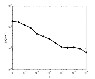
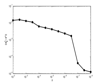
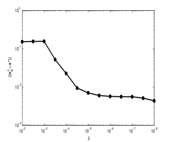
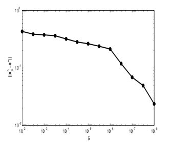
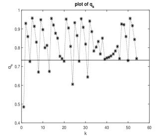
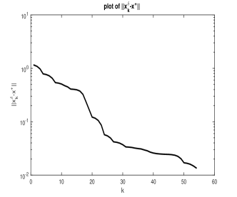
Further insight on the trust-region updating rule (5.41)-(5.42) can be gained analyzing the regularizing properties of the implemented trust-region strategy. First, we verified numerically that, though not explicitly enforced, the $q$-condition is satisfied in most of the iterations. As an illustrative example, we consider problem P2 with $\delta=10^{-4}$ and $x_{0}=0e$ and, in the left plot in Figure 1, we display the values $q_{k}=\frac{||J(x_{k}^{\delta})p_{k}+F(x_{k}^{\delta})||}{||F(x_{k}^{\delta})||}$ at the trust-region iterations, marked by an asterisk, and the value $q=1.1/\tau\approx 0.733$ fixed in our experiments, depicted by a solid line. We observe that, even if we have not imposed the $q$-condition, it is satisfied at most of the iterations. The plot on the right of Figure 1 shows a monotone decay of the error between $x_{k}^{\delta}$ and $x^{\dagger}$ through the iterations, which results to be in accordance with the theoretical results in Theorem 9. The regularizing properties of the implemented trust-region scheme are also shown in Figure 2 where, for each test problem we plot the error $||x_{k^{*}}^{\delta}-x^{\dagger}||$ for decreasing noise levels; it is evident that, in accordance with theory, the error decays as the noise level decreases.

Fig. 1: Regularizing trust-region applied to P2, $x_{0}=0e$, $\delta=10^{-4}$: values $q_{k}=\frac{||J(x_{k}^{\delta})p_{k}+F(x_{k}^{\delta})||}{||F(x_{k}^{\delta})||}$ (marked by an asterisk) and value of $q=1.1/\tau$ (solid line) versus the iterations (on the left); semilog plot of the error $||x_{k}^{\delta}-x^{\dagger}||$ versus the iterations (on the right).

Fig. 2: Regularizing trust-region applied to P1, $x_{0}=0e$ (top left), P2, $x_{0}=0e$ (top right), P3, $x_{0}=x_{0}(\alpha)=x_{0}(1.25)$ (lower left) and to P4, $x_{0}=x_{0}(\beta,\chi)=x_{0}(0.5,0)$ (lower right): log plot of the error $||x_{k^{*}}^{\delta}-x^{\dagger}||$ versus the noise $\delta$.

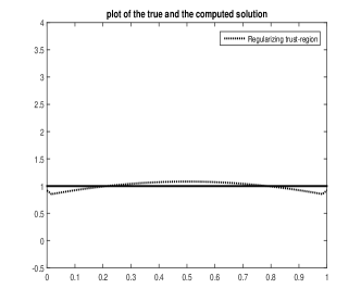
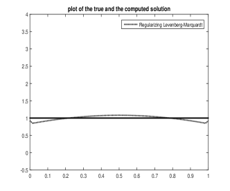
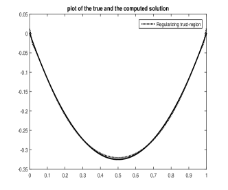
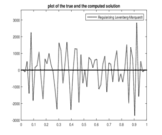
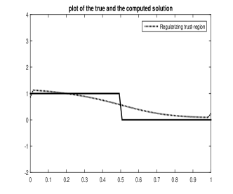
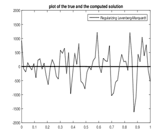
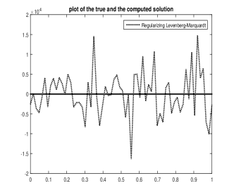
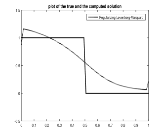
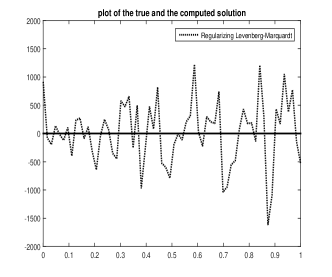
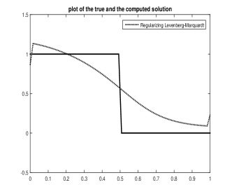
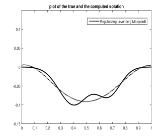
Let now compare the regularizing trust-region and Levenberg-Marquardt procedures. On runs successful for both methods, the two methods provide solutions of similar accuracy and such an accuracy increases with the vicinity of the initial guess to the true solution; as an example Figure 3 shows the solutions computed by the two methods for problems P1 and P3 for $\delta=10^{-2}$. On the other hand, for large noise $\delta$ and initial guesses farther from the true solution, for both methods the accuracy at the endpoints of the interval $[0,1]$ may deteriorate; for this occurrence we refer to Table 2 and runs on problems P1 and P2. Concerning failures, in 7 runs out of 32 the Levenberg-Marquardt algorithm does not act as a regularizing method as the generated sequence approaches a solution of the noisy problem. In Figure 4 we illustrate two unsuccessful runs of the Levenberg-Marquardt method; approximated solution computed by the regularizing trust-region and Levenberg-Marquardt procedures are shown for runs on problems P2 and P4.

Fig. 3: Regularizing trust-region (left) and regularizing Levenberg-Marquardt (right), true solution (solid line) and approximate solutions (dotted line). Upper part: P1, $\delta=10^{-2}$, $x_{0}=0e$; lower part: P3, $\delta=10^{-2}$, $x_{0}=x_{0}(\alpha)=x_{0}(1.25)$.

Fig. 4: True solution (solid line) and approximate solutions (dotted line) computed by the regularizing trust-region method (on the left) and the regularizing Levenberg-Marquardt method (on the right). Upper part: problem P2, $\delta=10^{-2},x_{0}=0e$; lower part: problem P4, $\delta=10^{-2},x_{0}=x_{0}(\beta,\chi)=x_{0}(0.5,0)$.

The overall experience on the Levenberg-Marquardt algorithm seems to indicate that the use of the $q$-condition is more flexible than condition (2.8) and provides stronger regularizing properties. In order to support this claim, in Figure 5 we report four solution approximations computed by the Levenberg-Marquardt algorithm for varying values of $q$, i.e. $q=0.67,0.70,0.73,0.87$. It is evident that the method is highly sensitive to the choice of the parameter $q$ and the quality of the solution approximation does not steadily improves as $q$ increases.

Fig. 5: Problem P4, $\delta=10^{-2}$, $x_{0}=x_{0}(\beta,\chi)=x_{0}(1.5,0)$: approximate solution computed by the regularizing Levenberg-Marquardt method for values of $q=0.67,\,0.70,\,0.73,\,0.87$.

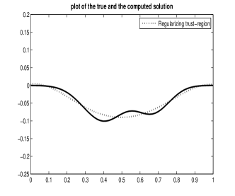
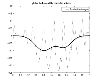
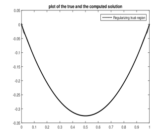
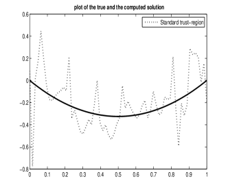
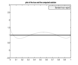
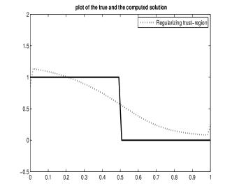
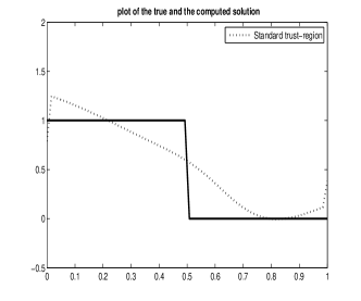
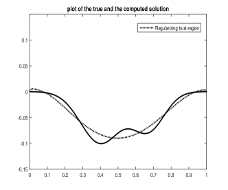
Fig. 6: True solution (solid line) and approximate solutions (dotted line) computed by the regularizing trust-region method (on the left) and the standard trust-region method (on the right). (a)-(b) problem P1, $\delta=10^{-2},x_{0}=0e$; (c)-(d) problem P2, $\delta=10^{-2},x_{0}=0e$; (e)-(f) problem P3, $\delta=10^{-2}$, $x_{0}=x_{0}(1.25)$; (g)-(h) problem P4, $\delta=10^{-2}$, $x_{0}=x_{0}(0.5,0)$.

We conclude this section considering the standard trust-region strategy. It is well known that the standard updating rule promotes the use of inactive trust-regions, at least in the late stage of the procedure. Clearly, this can adversely affect the solution of our test problems and our experiments confirmed this fact. In particular, for $\delta=10^{-2}$ and problems P1 and P2, the sequences computed by the standard trust-region method approach solutions of the noisy problem. The same behaviour occurs in most of the runs with P1 and P2 and noise level $\delta=10^{-4}$. Conversely, the approximations provided by the regularizing trust-region procedure are accurate approximations of true solutions in all the tests. Moreover, the approximations computed by the standard trust-region applied to problems P3 and P4 are less accurate than those computed by the regularizing trust-region although they do not show the strong oscillatory behavior arising in problems P1 and P2. In problem P4, this behavior is evident when the second, third and fourth starting guesses are used, while the approximation computed starting from the first initial guess is as accurate as the one computed by the regularizing trust-region. This good result of the standard trust-region on problem P4 with $x_{0}=x_{0}(1,1)$ is due to the fact that the trust-region is active in all iterations and therefore a regularizing behaviour is implicitely provided. As an example in Figure 6 we compare some solution approximations computed by the regularizing trust-region (left) and by the standard trust-region (right) with $\delta=10^{-2}$ applied to problem P1 (figures (a)-(b)), P2 (figures (c)-(d)), P3 (figures (e)-(f)) and P4 (figures (g)-(h)).

6 Conclusions

We have presented a trust-region method for nonlinear ill-posed systems, possibly with noisy data, where the regularizing behaviour is guaranteed by a suitable choice of the trust-region radius. The proposed approach shares the same local convergence properties as the regularizing Levenberg-Marquardt method proposed by Hanke in [10] but it is more likely to satisfy th discrepancy principle irrespective of the closeness of the initial guess to a solution of (1.1). The numerical experience presented confirms the effectiveness of the trust-region radius adopted and the regularizing properties of the resulting trust-region method. It also enlights that the new approach is less sensitive than the regularizing Levenberg-Marquardt method to the choice of the parameter $q$ in (2.8) and (2.18). Finally, as expected the numerical results show that the solution of the noisy problems may be misinterpreted by the standard trust-region method.

References

• [1] S.  Bellavia, C.  Cartis, N.  I.  M.  Gould, B. Morini, and Ph. L. Toint, Convergence of a Regularized Euclidean Residual Algorithm for Nonlinear Least-Squares, SIAM Journal on Numerical Analysis, 48, pp. 1–29, 2010.
• [2] C. Cartis, N. I. M. Gould, and Ph. L. Toint, Trust-region and other regularizations of linear least-squares problems, BIT, 49, pp. 21–53, 2009.
• [3] A.R. Conn, N.I.M. Gould, Ph.L. Toint, Trust-region methods, SMPS/SIAM Series on Optimization, 2000.
• [4] E. de Sturler, M. Kilmer, A regularized Gauss-Newton trust-region approach to imaging in diffuse optical tomography, SIAM Journal on Scientific Computing, 34, pp. 3057–3086, 2011.
• [5] J.Y Fan, J.Y Pan, A modified trust-region algorithm for nonlinear equations with updating rule for trust-region radius, International Journal of Computer Mathematics, 87, pp. 3186-3195, 2010.
• [6] J.Y. Fan, Y.X. Yuan, A new trust-region algorithm with trust-region radius converging to zero, Proceedings of the 5th International Conference on Optimization: Techniques and Applications, Hong Kong, 2001, pp. 786–794.
• [7] J.Y. Fan, J.Y. Pan, An improved trust-region algorithm for nonlinear equations, Computational Optimization and Applications, 48, pp. 59-70, 2011.
• [8] M.G. Gasparo, A. Papini, A. Pasquali, A two-stage method for nonlinear inverse problems, Journal of Computational and Applied Mathematics, 198, pp. 471-482, 2007.
• [9] C.V. Groetsch, The theory of Tikhonov regularization for Fredholm equations of the first kind, Pitman Advanced Publishing Program, Boston, 1984.
• [10] M. Hanke, Regularizing Levenberg-Marquardt scheme, with applications to inverse groundwater filtration problems, Inverse Problems, 13, pp. 79–95, 1997.
• [11] M. Hanke, The regularizing Levenberg-Marquardt scheme is of optimal order,J. Integral Equations Applications, 22, pp. 259–283, 2010.
• [12] P. Henrici, Elements of Numerical Analysis, J. Wiley and Sons, Chicester and New York, 1964.
• [13] B. Kaltenbacher, Toward global convergence for strongly nonlinear ill-posed problems via a regularizing multilevel approach, Numerical Functional Analysis and Optimization, 27, pp. 637–665, 2006.
• [14] B. Kaltenbacher, A. Neubauer, O. Scherzer, Iterative Regularization Methods for nonlinear ill-posed problems, Walter de Gruyter, Berlin, 2008.
• [15] K. Levenberg, A method for the solution of certain nonlinear problems in least-squares, Quarterly Applied Mathematics, 2, pp. 164–168, 1944.
• [16] D. Marquardt, An Algorithm for least-squares estimation of nonlinear parameters, SIAM Journal Applied Mathematics, 11, pp. 431–441, 1963.
• [17] J.J. Moré, The Levenberg-Marquardt algorithm: implementation and theory, Proceedings of 7th Biennial Conference, University of Dundee, Dundee, 1977, pp. 105–116. Lecture Notes in Mathematics, Vol. 630, Springer, Berlin, 1978.
• [18] V.A. Morozov, On the solution of functional equations by the method of regularization, Soviet Mathematics Doklady, 7, pp. 414-417, 1996.
• [19] J. Nocedal, S.J. Wright, Numerical Optimization, Springer Series in Operations Research, 1999.
• [20] Ph.L. Toint, Nonlinear stepsize control, trust regions and regularizations for unconstrained optimization, Optimization Methods and Software, 28, pp. 82–95, 2013.
• [21] C. R. Vogel, A constrained least squares regularization method for nonlinear ill-posed problems, Siam Journal Control and Optimization, 28, pp. 34-49, 1990.
• [22] C. R. Vogel, Computational methods for inverse problems, SIAM, Frontiers in Applied Mathematics, Providence, 2002.
• [23] Y. Wang, Y. Yuan, Convergence and regularity of trust region methods for nonlinear ill-posed problems, Inverse Problems, 21, pp. 821–838, 2005.
• [24] Y. Wang, Y. Yuan, On the regularity of trust region-CG algorithm for nonlinear ill-posed inverse problems with application to image deconvolution problem, Science in China Ser.A, 46, pp. 312–325, 2003.
• [25] J.L. Zhang, Y. Wang, A new trust region method for nonlinear equations, Mathematical Methods of Operations Research, 58, pp. 283–298, 2003.