Surface photocurrent in electron gas over liquid He subject to quantizing magnetic field

Abstract

The photogalvanic effect is studied in electron gas over the liquid He surface with the presence of quantizing magnetic field. The gas is affected by the weak alternating microwave electric field tilted towards the surface normal. Both linear and circular photogalvanic effects are studied. The current occurs via indirect phototransition with the participation of ripplons emission or absorption. The photogalvanic tensor has strong resonances at the microwave frequency $\omega$ approaching to the frequencies of transitions between size-quantized subbands. The resonances are symmetric or antisymmetric, depending on a tensor component. Other resonances appear at $\omega\approx n\omega_{c}$, where $n$ being integer and $\omega_{c}$ is the cyclotron frequency. It is found that the latter resonances split to two peaks connected with emission or absorption of ripplons. The calculated photogalvanic coefficients are in accord with the experimental observed values.

Introduction

The stationery surface photocurrent (in other words, surface photogalvanic effect (SPGE)) appears along the border of isotropic homogeneous bounded medium under the action of tilted alternative electric field we4 , alper . This effect was also studied in size-quantized systems we5 -we_jetpl2 . Recently, SPGE attracted attention chep as a tentative source of the microwave-induced photoresponse oscillations in 2D electron gas over the liquid He surface (EGOHeS). The microwave-induced resistance oscillations (MIRO) were the subject of numerous publications (see, e.g., review dmitr ). In particular, this effect was studied theoretically Mon -Mon3 in relation to EGOHeS (the theory of EGOHeS, see e.g., shik_mon ).

SPGE can be considered as another source of the observed photoresponse oscillations manifesting itself without stationary in-plane electric field. The theory of SPGE in EGOHeS was developed in we3 for the case of no magnetic field.

The present paper is a continuation of we3 with accounting for a strong magnetic field ${\bf B}$ directed perpendicular to the He surface $(x,y)$. The forced progressive in-plane electron motion in a quantizing magnetic field is a result of the transitions between size-quantized subbands with synchronous directed in-plane transitions between the Landau states. The mathematical reflection of this idea is the second order optical transition probability with the participation of scattering, in particular, ripplon-induced scattering. The translational motion results from the interference of transition amplitudes caused by out- and in-plane components of alternating electric field. The scattering leads to a change of the in-plane electron momentum with a shift of the orbit center.

We will mainly follow the conditions of the experiment chep on MIRO. We consider the electron gas of low density ($\sim 10^{6}$ cm^-2) over the He3 or He4 surface. At such low density the electron gas is non-degenerate. The photon energy is chosen close to the distance between the ground and the first excited size-quantized electron states $\Delta$. The magnetic field is assumed to be weak enough so that the cyclotron quantum is some times less than $\Delta$.

The mentioned resonance works as a magnification factor for transitions via the intermediate state. The mechanism of SPGE can be illustrated as follows. The population of subbands changes in- or contra-phase with the normal component of the alternating field if the frequency exceeds or it is less than $\Delta/\hbar$ and has $\pi/2$ shift if $\hbar\omega=\Delta$. This fact, together with the phase shift of the in-plane field component, determines the current direction.

Problem formulation

The phenomenology of SPGE in a magnetic field ${\bf B}={\bf b}B\equiv B(0,0,b_{z})$ is determined by the relation for the current density

$${\bf j}=\alpha_{1}\mbox{Re}\Big{[}({\bf E}-{\bf n}({\bf nE}))({\bf nE^{*}})\Big{]}-\frac{i\alpha_{2}}{2}[{\bf n},[{\bf E},{\bf E^{*}}]]+$$

$$\alpha_{3}[({\bf E}-{\bf n}({\bf nE})),{\bf b}]({\bf nE^{*}})+\frac{i\alpha_{4}}{2}[[{\bf n},[{\bf E},{\bf E^{*}}]],{\bf b}],$$ (1)

where ${\bf n}$ is the outer normal to the quantum well, ${\bf E}(t)=\mbox{Re}({\bf E}e^{-i\omega t})$ is the uniform microwave electric field (${\bf E}=(E_{x},E_{y},E_{z})$ is its complex amplitude). Real parameters $\alpha_{i}$ are the functions of magnetic field value $B$; $\alpha_{1}$ and $\alpha_{3}$ correspond to linear and $\alpha_{2}$ and $\alpha_{4}$ - to circular photogalvanic effects, respectively. ”Drift” components $\alpha_{1}$ and $\alpha_{2}$ exist in the case of zero magnetic field, while the ”Hall” components $\alpha_{3}$ and $\alpha_{4}$ originate from the magnetic field action, change their signs with the magnetic field and vanish if ${\bf B}=0$.

The current components $\propto\alpha_{2},~{}\alpha_{4}$ can be treated similar to translational motion of a rotating wheel. Electromagnetic field spin flow $ic[{\bf EE}^{*}]$ ($c$ is speed of light) transfers its angular momentum to electrons as a moment of force. The friction converts this moment to the translational electron motion.

We will base on the same model of 2D EGOHeS as in we3 . Electrons are attracted to He via the dielectric image force and the normal static electric field which composes Coulomb-like states $\chi_{l}(z)$ with energies $\epsilon_{l}$. The cyclotron frequency is supposed to be much lower than the Bohr energy. The interaction of electrons with surface waves (ripplons) and the homogeneous alternating electric field leads to the stationary surface current with density ${\bf j}.$

Eq.(Problem formulation) for current contains additive contributions $\propto E_{z}E_{x}$ and $\propto E_{z}E_{y}$. The system under consideration is axially-symmetric. Hence, to determine all components of the photogalvanic tensor, one can find only $x$ component of the current.

To calculate the photocurrent, we will use the approach first suggested by Titeika titeica . According to this approach, if unpertubed electron states are localized, the current can be expressed via the transition probability between these states. For the $x$-component of the current density, one can write

$$j_{x}=\frac{2e}{S}\sum_{\beta,\beta^{\prime}}(X_{\beta}-X_{\beta^{\prime}})W_{\beta\rightarrow\beta^{\prime}}f(\varepsilon_{\beta})(1-f(\varepsilon_{\beta^{\prime}})),$$ (2)

where $W_{\beta\rightarrow\beta^{\prime}}$ is the probability of transitions (caused by perturbation) between the electron states with quantum numbers $\beta$ and $\beta^{\prime}$, $\varepsilon_{\beta}$ and $X_{\beta}$ are the energy and the center of localization, correspondingly, $f(\varepsilon_{\beta})$ is the Fermi function, $S$ is the system area, $e$ is the electron charge.

Let us choose the vector potential of magnetic field in the form of ${\bf A}=(0,Bx,0)$ when the electron states are localized in the $x$-direction. Electron states are described by a set of quantum numbers $\beta=(l,n,k_{y})$, $l$ is the number of size quantized level, $n$ is the Landau number, $k_{y}$ is the $y$-component of electron momentum:

$$|\beta\rangle=\frac{1}{\sqrt{Sa}}e^{ik_{y}y}\phi_{n}(\frac{x-X_{\beta}}{a})\chi_{l}(z),$$

where $\phi_{n}(\xi)$ are dimensionless oscillator functions, $X_{\beta}=-b_{z}a^{2}k_{y}$ is the localization center (the cyclotron orbit center), $a=\sqrt{c/|e|B}$ is the magnetic length (we set $\hbar=1$). These states have energies $\varepsilon_{\beta}=\varepsilon_{n}+\epsilon_{l}$,   where $\varepsilon_{n}=\omega_{c}(n+1/2)$ is the n-th Landau level ($n=0,1,...$), $\omega_{c}=|e|B/mc$ is the cyclotron frequency, $\epsilon_{l}$ is the $l$-th size quantization level ($l=1,2,...$. If image attraction to liquid He prevails $\epsilon_{l}=-1/(2ma_{B}^{2}l^{2})$,

$$\chi_{1}(z)=2z\exp{(-z/a_{B})}a_{B}^{-3/2},$$

$$\chi_{2}(z)=z(2-z/a_{B})\exp{(-z/2a_{B})}(2a_{B})^{-3/2},$$ (3)

where $a_{B}=\kappa/me^{2}$ is the effective Bohr radius, $\kappa=4\kappa_{1}(\kappa_{1}+\kappa_{2})/(\kappa_{2}-\kappa_{1}),\kappa_{1,2}$ are dielectric constants of gaseous and liquid helium. Note, that the functions (Problem formulation) can be used also in the presence of the normal static field, if to consider them as variational functions with fitting parameter $a_{B}$.

In our case transition probability $W_{\beta\rightarrow\beta^{\prime}}$ is determined by the interaction with a microwave field and ripplons with the Hamiltonian ${\cal H}_{int}(t)={\cal U}_{er}+{\cal F}(t)$. The Hamiltonian of electron-ripplon interaction ${\cal U}_{er}$ is

$$({\cal U})_{er}=S^{-1/2}\sum_{\bf q}J_{\bf q}(b_{-{\bf q}}^{+}+{\bf q}_{\bf q})V_{q}(z),$$ (4)

where

$$V_{q}(z)=\frac{1}{ma_{B}^{3}}\sqrt{\frac{q}{2\rho}\omega_{q}}\bar{V}_{q}(z);~{}~{}\bar{V}_{q}(z)=\frac{a_{B}^{2}}{z^{2}}(1-qzK_{1}(qz)),$$ (5)

$J_{\bf q}=e^{i{\bf qr}},~{}~{}{\bf r}=(x,y),~{}~{}b_{\bf q}^{+},~{}b_{\bf q}$ are the operators of creation and destruction of ripplon with wave vector ${\bf q}$ and frequency $\omega_{q}=q^{3/2}\sqrt{\sigma_{0}/\rho},\rho$ is is the liquid helium density, $\sigma_{0}$ is the helium surface tension coefficient. Interaction of electron with microwave field is given by

$${\cal F}(t) = \frac{ie}{2\omega}{\bf Ev}e^{-i\omega t}+h.c.\equiv\frac{1}{2}Ue^{-i\omega t}+h.c.;$$ (6)

$$U = \frac{ie}{\omega}{\bf Ev}=\frac{ie}{\omega}({\bf E_{\|}v_{\|}}+E_{z}v_{z}),$$ (7)

where ${\bf v}$ is the operator of electron velocity. In the first order on the interaction Hamiltonian, the contributions of $({\cal U})_{er}$ and ${\cal F}(t)$ to the transition probability are additive and do not produce the photocurrent. Hence, the transition amplitude should be searched in the second (mixed in $({\cal U})_{er}$ and ${\cal F}(t)$) order. In this order we have

$$W_{\beta\rightarrow\beta^{\prime}}=\frac{\pi}{2S}\sum_{{\bf q},\pm}(N_{q}+\frac{1}{2}\pm\frac{1}{2})\times$$

$$\Bigg{[}\delta(\varepsilon_{\beta,\beta^{\prime}}-\omega\mp\omega_{q})|({\cal B}_{\bf q})_{\beta\beta^{\prime}}|^{2}+$$

$$\delta(\varepsilon_{\beta,\beta^{\prime}}+\omega\mp\omega_{q})|(\tilde{{\cal B}}_{\bf q})_{\beta\beta^{\prime}}|^{2}\Bigg{]},$$ (8)

where

$$({\cal B}_{\bf q})_{\beta\beta^{\prime}}=\sum_{\beta_{1}}\Bigg{(}\frac{(I_{\bf q})_{\beta,\beta_{1}}U_{\beta_{1},\beta^{\prime}}}{\eta-i\omega+i\varepsilon_{\beta_{1},\beta^{\prime}}}+$$

$$\frac{U_{\beta\beta_{1}}(I_{\bf q})_{\beta_{1},\beta^{\prime}}}{\eta+i\omega+i\varepsilon_{\beta_{1},\beta}}\Bigg{)};~{}~{}~{}~{}~{}~{}~{}~{}~{}~{}~{}~{}~{}~{}(\eta=+0).$$ (9)

Here $I_{\bf q}=J_{\bf q}V_{q}(z),~{}~{}\varepsilon_{\beta,\beta^{\prime}}$ means $\varepsilon_{\beta}-\varepsilon_{\beta}^{\prime}$, $N_{q}$ is the ripplon equilibrium distribution function. Quantity $(\tilde{{\cal B}}_{\bf q})_{\beta\beta^{\prime}}$ is determined by Eq.(Problem formulation) with change $\omega\rightarrow-\omega$ and $U\rightarrow U^{+}$. For matrix elements $(I_{\bf q})_{\beta,\beta^{\prime}}$ one can write the following expressions:

$$(I_{\bf q})_{\beta,\beta^{\prime}}=(J_{\bf q})_{n,k_{y};n^{\prime},k_{y}^{\prime}}(V_{q})_{l,l^{\prime}},$$ (10)

where

$$(J_{\bf q})_{n,k_{y};n^{\prime},k_{y}^{\prime}}=$$

$$\delta_{X,X^{\prime}-a^{2}q_{y}}i^{|n-n^{\prime}|}e^{i(q_{x}X+b_{z}u_{q}\sin{(2\varphi)}/2)}e^{ib_{z}(n^{\prime}-n)\varphi}J_{nn^{\prime}}(u_{q});$$

$$J_{nn^{\prime}}(u_{q})=\sqrt{\frac{\min{(n,n^{\prime})!}}{\max{(n,n^{\prime})!}}}u_{q}^{|n-n^{\prime}|/2}e^{-u_{q}/2}L_{\min{(n,n^{\prime})}}^{|n-n^{\prime}|},$$ (11)

$L_{n}^{m}(u)$ is the generalized Laguerre polynomial, $u_{q}=q^{2}a^{2}/2$, $\varphi$ is the polar angle of vector ${\bf q}~{}~{}(q_{x}=q\cos{\varphi},q_{y}=q\sin{\varphi});~{}~{}(V_{q})_{l,l^{\prime}}=\int_{0}^{\infty}dzV_{q}(z)\chi_{l}(z)\chi_{l^{\prime}}(z)$. We will consider the PGE at resonance conditions, when the microwave frequency is close to the distance between size-quantization subbands $l=1$ and $l=2$. The expressions for the necessary quantities $(V_{q})_{1,1},~{}(V_{q})_{2,2}$ and $(V_{q})_{1,2}$ can be found, for example, in we3 .

The matrix elements of operator $U$ are

$$U_{\beta,\beta^{\prime}}=\frac{ie}{\omega}\delta_{X,X^{\prime}}\Big{[}\delta_{l,l^{\prime}}\frac{a\omega_{c}}{\sqrt{2}}\Big{(}(iE_{x}+b_{z}E_{y})\sqrt{n}\delta_{n,n^{\prime}+1}+$$

$$(-iE_{x}+b_{z}E_{y})\sqrt{n^{\prime}}\delta_{n^{\prime},n+1}\Big{)}+\delta_{n,n^{\prime}}E_{z}(v_{z})_{l,l^{\prime}}\Big{]}$$ (12)

Using Eqs.(10), (Problem formulation) and (Problem formulation) we get for PGE current:

$$j_{x}=-\frac{2e}{2\pi a^{2}}\frac{e^{2}a^{2}b_{z}}{\omega^{2}}\frac{2\pi a\omega_{c}}{2\sqrt{2}S}\times$$

$$\sum_{{\bf q},\pm}\sum_{n,l;n^{\prime},l^{\prime}}f(\varepsilon_{n,l})(1-f(\varepsilon_{n^{\prime},l^{\prime}}))J_{n,n^{\prime}}\big{(}N_{q}+\frac{1}{2}\pm\frac{1}{2}\big{)}q_{y}V_{l,l^{\prime}}$$

$$\times\Bigg{\{}\delta(\varepsilon_{n,n^{\prime}}+\epsilon_{l,l^{\prime}}-\omega\mp\omega_{q})\times$$

$$\mbox{Re}\Big{[}E_{z}^{*}\sum_{l_{1}}\Big{(}\frac{V_{l,l_{1}}(v_{z})_{l_{1},l^{\prime}}}{\eta-i\omega+\epsilon_{l_{1},l^{\prime}}}+\frac{(v_{z})_{l,l_{1}}V_{l_{1},l^{\prime}}}{\eta+i\omega+\epsilon_{l_{1},l}}\Big{)}^{*}\times$$

$$i\ \mbox{sig}(n^{\prime}-n)\Big{(}e^{ib_{z}\varphi}E_{-}\frac{\sqrt{n^{\prime}+1}J_{n,n^{\prime}+1}-\sqrt{n}J_{n-1,n^{\prime}}}{\omega_{c}-\omega}-$$

$$e^{-ib_{z}\varphi}E_{+}\frac{\sqrt{n^{\prime}}J_{n,n^{\prime}-1}-\sqrt{n+1}J_{n+1,n^{\prime}}}{\omega_{c}-\omega}\Big{)}\Big{]}+$$

$$(\omega\rightarrow-\omega,{\bf E}\rightarrow{\bf E}^{*})\Bigg{\}},$$ (13)

where $E_{\pm}=E_{x}\pm ib_{z}E_{y},\ \varepsilon_{n,n^{\prime}}=\omega_{c}(n-n^{\prime}),\ \epsilon_{l,l^{\prime}}=\epsilon_{l}-\epsilon_{l^{\prime}}$, $\mbox{sig}(x)=\mbox{sgn}(x+0)$.

Quantities $J_{n,n^{\prime}}$ justify the relations:

$$(\sqrt{n^{\prime}+1}J_{n,n^{\prime}+1}-\sqrt{n}J_{n-1,n^{\prime}})\mbox{sig}(n^{\prime}-n)=\sqrt{u_{q}}J_{n,n^{\prime}}~{}~{}~{}$$

$$(\sqrt{n^{\prime}}J_{n,n^{\prime}-1}-\sqrt{n+1}J_{n+1,n^{\prime}})\mbox{sig}(n^{\prime}-n)=\sqrt{u_{q}}J_{n,n^{\prime}}.~{}~{}$$ (14)

Using Eq.(Problem formulation) one can rewrite Eq.(Problem formulation) in the form

$$j_{x}=\frac{e^{3}a\omega_{c}}{2\sqrt{2}\pi\omega^{2}}\sum_{\pm}\sum_{n,l;n^{\prime},l^{\prime}}f(\varepsilon_{n,l})(1-f(\varepsilon_{n^{\prime},l^{\prime}}))\times$$

$$\int\limits_{0}^{\infty}dqq^{2}J_{n,n^{\prime}}^{2}\sqrt{u_{q}}\big{(}N_{q}+\frac{1}{2}\pm\frac{1}{2}\big{)}V_{l,l^{\prime}}\times$$

$$\Bigg{\{}\delta(\varepsilon_{n,n^{\prime}}+\epsilon_{l,l^{\prime}}-\omega\mp\omega_{q})\times$$

$$\mbox{Re}\Big{[}\sum_{l_{1}}\Big{(}\frac{V_{l,l_{1}}(v_{z})_{l_{1},l^{\prime}}}{\eta-i\omega+\epsilon_{l_{1},l^{\prime}}}+\frac{(v_{z})_{l,l_{1}}V_{l_{1},l^{\prime}}}{\eta+i\omega+\epsilon_{l_{1},l}}\Big{)}^{*}E_{z}^{*}$$

$$\times\frac{\omega_{c}E_{x}-ib_{z}\omega E_{y}}{\omega_{c}^{2}-\omega^{2}}\Big{]}+(\omega\rightarrow-\omega,{\bf E}\rightarrow{\bf E}^{*})\Bigg{\}}.$$ (15)

Because of low electron concentration, function $f(\varepsilon)=e^{(\mu-\varepsilon)/T}$ is the Boltzmann distribution function ($\mu$ being the chemical potential), $f\ll 1$. We will consider the resonance case when microwave frequency is close to the distance between subbands with $l=1$ and $l=2$. Assuming that $\Delta\gg T$ and leaving only resonance terms one can reduce Eq.(Problem formulation) to:

$$j_{x}=\frac{n_{e}e^{3}z_{12}\Delta a(1-e^{-\omega_{c}/T})}{2\sqrt{2}m\omega^{2}(\omega_{c}^{2}-\omega)}\sum_{\pm,n,n^{\prime}}e^{-n\omega_{c}/T}\int\limits_{0}^{\infty}dqq^{2}J_{n,n^{\prime}}^{2}$$

$$\times\sqrt{u_{q}}\big{(}N_{q}+\frac{1}{2}\pm\frac{1}{2}\big{)}V_{1,1}\mbox{Im}\Bigg{\{}E_{z}^{*}(\omega_{c}E_{x}-ib_{z}\omega E_{y})\times$$

$$\Big{[}\frac{V_{1,2}}{\eta-i\delta}\delta(\omega_{c}(n-n^{\prime})-\omega\mp\omega_{q})+$$

$$\frac{V_{1,2}}{\eta+i\delta}\delta(\omega_{c}(n-n^{\prime})+\omega\mp\omega_{q})+$$

$$\Big{(}\frac{V_{1,1}}{\eta-i\delta}+\frac{V_{2,2}}{\eta+i\delta}\Big{)}\delta(\omega_{c}(n-n^{\prime})-\delta\mp\omega_{q})\Big{]}\Bigg{\}}.$$ (16)

Here $\Delta=\epsilon_{2}-\epsilon_{1},~{}\delta=\Delta-\omega$ is the resonance detuning, $n_{e}$ is the electron density.

At the fulfilment of condition $\omega_{c}\gg T$ Eq.(Problem formulation) can be simplified:

$$j_{x}=\frac{CF}{\delta^{2}+\eta^{2}}\Big{[}\mbox{Re}(E_{x}E_{z}^{*})\omega_{c}\delta+\mbox{Im}(E_{x}E_{z}^{*})\omega_{c}\eta-$$

$$\mbox{Re}(E_{y}E_{z}^{*})b_{z}\omega\eta+\mbox{Im}(E_{y}E_{z}^{*})b_{z}\omega\delta\Big{]},$$ (17)

where

$$F=\sum_{n}\Big{[}\big{(}N_{q}+1\big{)}\theta(\omega-n\omega_{c})+N_{q}\theta(n\omega_{c}-\omega)\Big{]}\times$$

$$\Big{(}\frac{\omega_{q}}{\omega}\Big{)}^{4/3}\frac{1}{n!}u_{q}^{n}e^{-u_{q}}\bar{V}_{1,1}(qa_{B})\bar{V}_{1,2}(qa_{B})\Bigg{|}_{\omega_{q}=|\omega-n\omega_{c}|},~{}~{}$$ (18)

$$C=\frac{n_{e}e^{3}z_{12}\Delta a^{2}\rho^{2/3}}{12m^{3}a_{B}^{6}\omega^{2/3}(\omega^{2}-\omega_{c}^{2})\sigma_{0}^{5/3}},~{}~{}~{}~{}~{}~{}~{}~{}~{}~{}~{}~{}~{}~{}~{}~{}~{}~{}~{}~{}~{}~{}~{}~{}~{}$$ (19)

$u_{q}=\omega_{q}^{4/3}(\rho/\sigma_{0})^{2/3}a^{2}/2,~{}~{}qa_{B}=\omega_{q}^{2/3}(\rho/\sigma_{0})^{1/3}a_{B}.$

For $\bar{V}_{ij}(y)$ we have
$\bar{V}_{11}(y)=2y^{2}(y^{2}-4)^{-3/2}\Big{[}(y^{2}-4)^{1/2}-2\arccos(2/y)\Big{]},$ $\bar{V}_{12}(y)=(8y^{2}\sqrt{2}/9)(4y^{2}-9)^{-5/2}\Big{[}(4y^{2}-9)^{1/2}(9+8y^{2})-36y^{2}\arccos(3/(2y))\Big{]}.$

The comparison of Eq.(Problem formulation) with Eq.(Problem formulation) gives for the photogalvanic coefficients $\alpha_{i}=CFa_{i}$:

$$a_{1}=\frac{\omega_{c}\delta}{\eta^{2}+\delta^{2}},~{}a_{2}=\frac{\omega_{c}\eta}{\eta^{2}+\delta^{2}},$$

$$~{}a_{3}=\frac{\omega\eta}{\eta^{2}+\delta^{2}},~{}a_{4}=\frac{\omega\delta}{\eta^{2}+\delta^{2}}.$$ (20)

Eq.(18) has been obtained neglecting the Landau level widths. We have remained the widening $\eta$ of the intersubband distances in the prefactors $a_{i}$ only to get the finite result. To include the Landau level widths, one should blur the delta-functions under the integral in Eq.(18) as $\delta(x)\to\eta_{1}/(x^{2}+\eta_{1}^{2})/\pi$. In principle, widths $\eta$ and $\eta_{1}$ may be different, but here we will suppose $\eta_{1}=\eta$.

Thus, the dependence of the photogalvanic coefficients on the magnetic field is mainly determined by the function $F$. Fig. 1 shows this function in the case of zero electron level widths. For numerical calculations we used the parameters of He3 and electron gas close to the conditions of experiment chep : $\kappa_{1}=1,\kappa_{2}=1.057$, $\rho=0.082$g/cm^-3, $\sigma_{0}=0.1553$erg/cm^-2 and $n_{e}=1.4\cdot 10^{6}$cm^-2. The parameter $a_{B}=8.7\cdot 10^{-7}$cm is chosen to fit the intersubband distance $\Delta=0.38$ meV corresponding to the experiment chep . The dependence of $F(B)$ contains narrow twin peaks in the vicinity of cyclotron resonance harmonics $\omega=n\omega_{c}$. At high temperature, the left and right peaks have the same amplitudes. With the drop of temperature, the right peak is suppressed as compared to the left one. The way the widening of electron levels affect the shape of resonances is demonstrated in Fig.2 - Fig.4.

Figure 1: Function $F$ versus magnetic field at $T=0.2$K. The widening of the Landau levels is neglected. The double peaks correspond to $\omega=n\omega_{c}$ for $n=8,7,6,5,4$ (from left to right). Insert: the fine structure of e double peak $n=5$ at different temperatures.

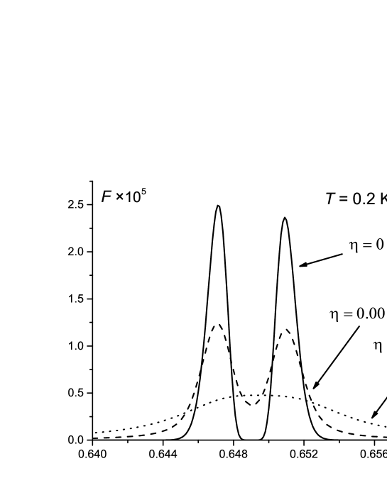
Figure 2: Fig.2. The evolution of $F$ versus magnetic field with the change of the Landau level width in the region of peak $\omega/\omega_{c}=5$. The widening smears the twin structure.

Figure 3: Fig.3. The same as in Fig.2 for $T=0.03$K.

Figure 4: Fig.4. The same as in Fig.2 for $T=0.01$K.

Analysis of results

The photocurrent dependence on the parameters has a huge ”zoo” of resonances. First, this is the resonance $\hbar\omega\approx\Delta$ in coefficients $a_{i}$ (see Eq.(Problem formulation)). This resonance originates from the participation of $E_{z}$ component in transitions and it is not specific for the case with magnetic field. According to our previous papers, this resonance appears due the intermediate state. It determines the symmetric or antisymmetric behavior of PGE coefficients in the vicinity of resonance frequency, depending on the kind of electromagnetic field polarization (linear or circular). In addition to SPGE coefficients existing also at $B=0$ we3 , the magnetic field leads to the Hall photocurrent component appearance.

Another resonance is the cyclotron resonance when the frequency of external field coincides with the cyclotron frequency. In the domain of parameters which we concentrate here this resonance is far from our focus (and the experimental situation in chep ).

One more kind of resonances is the cyclotron resonance harmonics $\omega\approx n\omega_{c}$ (corresponding to magnetic fields $B_{n}=m\Delta c/en$) on which we focus our attention (see Fig.1). These resonances originate from the participation of the scattering in the transition processes induced by alternating electric field. Scattering violates the linear character of cyclotron motion resulting in cyclotron harmonics. Such resonances are typical for MIRO.

According to Eq. (Problem formulation), the maxima (as functions of detuning $\delta)$ of the Hall components of the photogalvanic tensor $\alpha_{3},~{}\alpha_{4}$ exceed corresponding drift components $\alpha_{1},~{}\alpha_{2}$: $\max_{\delta}(\alpha_{1}):\max_{\delta}(\alpha_{2}):\max_{\delta}(\alpha_{3}):\max_{\delta}(\alpha_{4})=0.5:1:n:0.5n$, where $\omega=n\omega_{c}$. This is typical situation for transport in a strong magnetic field where the drift along the drawing force is weaker than in the Hall direction. The maximal values of symmetric resonances are 2 times larger than antisymmetric ones.

In fact, these resonances are twinned (see insert to Fig.1). Note, that in quasielastic approximation the resonances should be solitary. For example, this is the case when impurity scattering is take into account only. In the considered situation of ripplon scattering the resonance splitting originates from the energy of emitted or absorbed ripplon $\omega_{q}=|n\omega_{c}-\omega|$. At $B\to B_{n}$, $\omega_{q}\to 0$, hence the process probability vanishes. In particular, if the temperature is relatively high, $T>\omega_{q}$, $F(B)\propto|B-B_{n}|^{4n/3+3}\ln(1/|B-B_{n}|)$. This explains deep dips between the twin peaks at $n\omega_{c}=\omega$.

On the other hand, the peaks splitting can be estimated as $\sqrt{\sigma_{0}/\rho}(2n+9/2)^{3/4}n^{-7/4}(m\Delta)^{3/4}2mc/e$. This estimate is consistent with insert to Fig 1. The left and right peaks in pairs correspond to ripplons emission/absorption, accordingly. Their height ratio is $(N_{q}+1)/N_{q}$. At a $T\gg\omega_{q}$ the peaks heights equalize and behave $\propto T$; when $T\to 0$ both peaks go down, but the left one tends to constant, while the right one is suppressed $\propto\exp{(-\omega_{q}/T)}$.

In the aforesaid specific conditions corresponding to chep the parameter $C$ has the value $C=-88$ pA$\cdot$cm/V² at $n=5$. If to suppose the level width $\eta=10^{-4}\Delta$ and $T=0.2$K this yields maximum of photogalvanic coefficient $\max_{\delta}(\alpha_{3})=2.5\max_{\delta}(\alpha_{1})=5\max_{\delta}(\alpha_{2})=2.5\max_{\delta}(\alpha_{4})=2.2$pA$\cdot$cm/V² achieved at magnetic field $B=0.647$T. These values are commensurable with the order of MIRO oscillations in chep .

In conclusion, we have found the value of photocurrent along the charged liquid helium surface affected by tilted alternating electric field in the presence of vertical magnetic field. Different photogalvanic coefficients represent responses to the linear and circular polarization of drift (invariant with respect to the sign of magnetic field) and Hall (proportional to this sign) currents. The ripplon scattering mechanism was taken into account. SPGE coefficients have (symmetric or antisymmetric) their resonant behavior when the field frequency approaches the intersubband one. Besides, resonances on the cyclotron harmonics are observed. The current value is consistent with that observed in the experiment.

References

• (1) L.I.Magarill and M.V.Entin, Fiz. Tverd. Tela (Leningrad) 21, 1280 (1979) [Sov. Phys. Sol. State 21, 743 (1979)].
• (2) V.L.Al’perovich. V.I.Belinicher, V.N.Novikov, and A.S.Terekhov, Zh. Eksp. Teor. Fiz. 80, 2298 (1981) [Sov. Phys. JETP 53, 1201 (1981)].
• (3) L.I.Magarill and M.V.Entin, Poverkhnost’. Fizika, khimiya, mekhanika, 1, 74 (1982).
• (4) G.M.Gusev, Z.D.Kvon, L.I.Magarill, A.M.Palkin, V.I.Sozinov, O.A.Shegai, and V.M.Entin, JETP Lett. 46, 33 (1987).
• (5) V.M.Entin, L.I.Magarill, Pis’ma v ZhETP 97, 737 (2013) [JETP Lett., 97, 639 (2013)].
• (6) V.M.Entin, L.I.Magarill, Pis’ma v ZhETP 98, 43 (2013) [JETP Lett., 98, (2013)].
• (7) D.Konstantinov, A.Chepelyanskii, and K.Kono, Journal Physical Society of Japan 81, 093601 (2012).
• (8) I.A.Dmitriev, A.D.Mirlin, D.G.Polyakov, and M.A.Zudov, Review of Modern Physics, v.84 (2012).
• (9) Yu.P.Monarkha, Low Temp. Phys. 37, 655 (2011).
• (10) Yu.P.Monarkha, Low Temp. Phys. 38, 451 (2012).
• (11) Yu.P.Monarkha, Arxiv 1401.5883 [cond-mat.mes-hall] (2014).
• (12) V.B.Shikin and Yu.P.Monarkha, Journal of Low Temperature Physics, 16, 193 (1974). Yu.P.Monarkha and V.B.Shikin, Fizika nizkikh temperatur (in Russian), 8, 563 (1982).
• (13) M.V.Entin, L.I.Magarill, Pis’ma v ZhETP 97, 737 (2013) [JETP Lett., 98, 919 (2013)].
• (14) S.Titeica, Ann.d. Phys., 22, 128 (1935).