Wide Field Multiband Imaging of Low Redshift Quasar Environments

Abstract

We present photometry of the large scale environments of a sample of twelve broad line AGN with $0.06<z<0.37$ from deep images in the SDSS $u$, $g$, $r$, and $i$ filters taken with the 90Prime prime focus camera on the Steward Observatory Bok Telescope. We measure galaxy clustering around these AGN using two standard techniques: correlation amplitude (B_gq) and the two point correlation function. We find average correlation amplitudes for the 10 radio quiet objects in the sample equal to (9$\pm$18, 144$\pm$114, -39$\pm$56, 295$\pm$260) Mpc^1.77 in ($u$, $g$, $r$, $i$), all consistent with the expectation from galaxy clustering. Using a ratio of the galaxy-quasar cross-correlation function to the galaxy autocorrelation function, we calculate the relative bias of galaxies and AGN, $b_{gq}$. The bias in the $u$ band, $b_{gq}=3.08\pm 0.51$ is larger compared to that calculated in the other bands, but it does not correlate with AGN luminosity, black hole mass, or AGN activity via the luminosity of the [O III] emission line. Thus ongoing nuclear accretion activity is not reflected in the large scale environments from $\sim$10 $h^{-1}$ kpc to $\sim$0.5 $h^{-1}$ Mpc and may indicate a non-merger mode of AGN activity and/or a significant delay between galaxy mergers and nuclear activity in this sample of mostly radio quiet quasars.

1. Introduction

In local galaxies, the masses of the nuclear black holes are correlated with the stellar velocity dispersion of the host galaxy bulges, the M_BH-$\sigma$ relation (Ferrarese & Merritt, 2000; Gebhardt et al., 2000; Tremaine et al., 2002; McLure & Dunlop, 2002; Marconi & Hunt, 2003). The host galaxies of low redshift ($z$$<$0.4) quasars are consistent with these correlations, with the most powerful quasars typically inhabiting massive, early-type galaxies (McLeod & Rieke, 1995; McLeod et al., 1999; McLure et al., 1999; Hamilton et al., 2002; Dunlop et al., 2003; Floyd et al., 2004).

Theoretical modeling establishes a framework for the coevolution of galaxies and supermassive black holes such that after the initial formation of central black holes in galaxies, nuclear activity and star formation are triggered by a merger event (Barnes & Hernquist, 1992; Kauffmann & Haehnelt, 2000; Volonteri et al., 2003; Wyithe & Loeb, 2003; Granato et al., 2004; Haiman et al., 2004; Di Matteo et al., 2005; Springel et al., 2005a, b; Croton et al., 2006; Hopkins et al., 2006a, b, 2008; Somerville et al., 2008). These hierarchical models make specific predictions for the large scale environments of luminous quasars.

Observational studies have investigated the wide parameter space of this problem by examining: the quasar-quasar and galaxy-quasar clustering in terms of correlation length and amplitude; nearest neighbor and other statistics for estimating environment density; properties of galaxies in AGN environments; and the properties of AGN host galaxies, covering also a range in redshift and intrinsic AGN properties. Many of these studies have used Sloan Digital Sky Survey (SDSS) data, thus concentrating on the $z\lesssim 0.3$ universe.

From the observational results, two points of consensus have emerged that generally agree with the models: (1) AGN activity is associated with galaxy mergers and enhanced star formation in their hosts (Sanders et al., 1988; Kauffmann et al., 2004; Guyon et al., 2006; Canalizo et al., 2007; Bennert et al., 2008; Coil et al., 2009; Veilleux et al., 2009; Teng & Veilleux, 2010), although there is increasing evidence, e.g. due to lack of correlation of galaxy structural parameters with local environment density, (Kauffmann et al., 2004) and an absence of increased rate of disturbed host morphologies in AGN hosts up to $z\sim 1.3$,(Grogin et al., 2005; Gabor et al., 2009), that the onset of nuclear activity is delayed with respect to the initial galaxy interaction (Li et al., 2006, 2008; Ellison et al., 2013) and that there is a significant non-merger mode to AGN activity (Hopkins & Hernquist, 2006); (2) on megaparsec scales, bright AGN cluster like L^∗ galaxies (Adelberger & Steidel, 2005; Li et al., 2006; Serber et al., 2006; Coldwell & Lambas, 2006; Coil et al., 2007; Gilli et al., 2009), and over time, they occupy dark matter halos of constant mass ($\sim 2-3\times 10^{12}$ $h^{-1}$ M_⊙) so they were more biased tracers of mass at higher redshift than they are in the current epoch (Porciani et al., 2004; Wake et al., 2004; Croom et al., 2005; Myers et al., 2006, 2007a; Shen et al., 2007; Ross et al., 2009).

Quasar-quasar clustering shows little or no dependence on quasar luminosity (Croom et al., 2005; Porciani & Norberg, 2006; Myers et al., 2006, 2007a; Shen et al., 2009) except at the lowest redshifts (Wake et al., 2004; Constantin & Vogeley, 2006). Galaxy clustering around AGN does correlate with nuclear activity especially for luminous, strongly accreting AGN, which tend to lie in massive hosts ($M^{*}\gtrsim 3\times 10^{10}M_{\odot}$) with higher than average SFR (Kauffmann et al., 2003), and are more likely to be found in lower density environments (Kauffmann et al., 2004; Constantin et al., 2008; Silverman et al., 2009; Sabater et al., 2012, 2013). No quasar luminosity dependence on galaxy-quasar clustering is seen in the DEEP2 sample with $z\sim 1$ (Coil et al., 2007), though quasars are found to cluster like blue, star-forming galaxies.

AGN fueling via a merger-independent quiescent or Seyfert mode (Hopkins & Hernquist, 2006) may be most important for weaker AGN, as they show no preference for low density regions in low redshift samples (Kauffmann et al., 2004) and X-ray selected AGN at $z\sim 1$ with lower mass hosts ($M^{*}\lesssim 10^{11}M_{\odot}$) which are found in a broad range of environments (Silverman et al., 2009). However, there is evidence that the transition from Seyferts to LINERS proposed by Kewley et al. (2006) is affected by the density of the environment, in SDSS samples at low redshift (Constantin et al., 2008) and in the X-ray selected $z\sim 1$ AGN sample of Montero-Dorta et al. (2009). These authors, and Constantin & Vogeley (2006) also find that that the LINERS cluster more strongly than Seyfert galaxies.

Unlike galaxies, quasars do show excess clustering on small scales (10-100 $h^{-1}$ kpc) up to $z\sim 3$ (Hennawi et al., 2006; Myers et al., 2007b; Shen et al., 2010). And while studies of the $\sim$1 $h^{-1}$ Mpc environments around low redshift AGN show no distinct correlation between nuclear activity and the presence of galaxy neighbors on these scales (Serber et al., 2006; Coldwell & Lambas, 2006; Li et al., 2008), there is evidence that the presence of a galaxy companion on smaller scales does influence AGN activity (Alonso et al., 2007; Sabater et al., 2013). On larger scales, $z\gtrsim 1$ radio loud quasars are found in richer environments than radio quiet objects (Hall et al., 1998; Teplitz et al., 1999; Wold et al., 2003) while for low redshift this distinction is less pronounced and AGN generally are not preferentially found at the centers of rich clusters (Fisher et al., 1996; Croom & Shanks, 1999; McLure & Dunlop, 2001b; Wold et al., 2001; Coldwell et al., 2002; Barr et al., 2003; Coldwell & Lambas, 2006). For cold, or QSO, mode accretion, this can be understood as inhibition due to the stripping and harassment that occurs in these environments. However, some studies have shown that quasars do trace the large scale structure of galaxy clusters (Söchting et al., 2002, 2004; Gilli et al., 2003; Silverman et al., 2008) on scales up to 10 $h^{-1}$ Mpc.

In this paper, we investigate the large scale environments of a sample of 12 relatively bright low redshift ($0.06<z<0.37$) broad line AGN using deep images in the SDSS $u$, $g$, $r$, and $i$ filters. The fields presented here overlap almost entirely with the SDSS, but our photometry goes significantly deeper, in some fields and filters by up to 2.5-3 magnitudes. Our wide field multiband study on scales $\sim$1 degree, is distinct from previous single filter studies with Hubble Space Telescope (HST) using the $\sim$3 arcminute field of the Wide Field Planetary Camera 2 (Fisher et al., 1996; Finn et al., 2001; McLure & Dunlop, 2001b). Likewise, the multiband nature of our study extends previous wider field studies using the B_J and R data from UK Schmidt plates (Brown et al., 2001; Coldwell et al., 2002; Söchting et al., 2002). This study is a blend of a statistical approach and a detailed study of each field. We calculate the correlation lengths and amplitudes of the galaxy-quasar clustering and compare results in different bands. We also use our data and results from the literature to discuss each quasar’s environment in detail. Our primary aim is to probe galaxies as far down the luminosity function as allowed by the depth of the photometry to as wide an area around each quasar as possible in order to test if galaxy clustering around quasars is comparable to that of galaxy-galaxy clustering to these depths at these scales. Throughout this paper we assume a cosmology with $h=0.71$ ($H_{0}=100$ h km s^-1 Mpc^-1), $\Omega_{m}=0.27$, and $\Omega_{\Lambda}=0.73$.

2. Data

2.1. Observations and Reductions

We made our observations with the 90Prime prime focus imager (Williams et al., 2004) on the 2.3-meter Bok Telescope at Kitt Peak National Observatory in January - June, 2008. 90Prime is a wide field camera consisting of four CCDs arranged in a square mosaic located at the prime focus of the telescope with a field of view of $\sim$1 degree. We used the SDSS $u$, $g$, $r$, and $i$ filters for the photometry, and with the exception of HS0624+690, all our fields lie inside the SDSS footprint. However, our photometry is significantly deeper than that of the SDSS survey, as discussed further in the next section. We chose the quasars in our sample to have galaxy environments accessible to deep imaging with our 2-meter class telescope and with ultraviolet spectra in the archives of the Hubble Space Telescope or Far Ultraviolet Spectroscopic Explorer for future studies of line of sight and associated absorption in these systems. The lower bound on the redshifts of the sample quasars was determined by the size of the chips in the CCD mosaic and the $\sim$Mpc scales targeted in this study. We compiled a sample of $\sim$20 target fields for the first semester of the 2008 observing season and completed the photometry in at least two bands for 12 of those fields. Total exposure times were estimated for each field and filter in order to achieve significant detections of galaxies with M${}^{*}+2$ at redshift of the quasar in each filter. The final sample presented here includes one Seyfert, 9 radio quiet quasars and two radio loud quasars and so somewhat overrepresents the radio loud population, although we separate these fields out in the discussion of our results. Follow up observations to obtain data on other fields of quasars with available UV spectra and with appropriate redshifts are possible.

The quasars themselves were centered on one of the chips of the mosaic, usually chip 1, rather than in the center of the field due the 8.3′ interchip gaps and several traps and other quality issues with the other chips in the mosaic at the time of the observations. The raw data frames are multiextension FITS files consisting of eight 2048$\times$4096 images, one for each of the two amplifiers on each chip. Amplifiers 1 and 2 lie on chip 1, 3 and 4 on chip 2, 5 and 6 on chip 3, and amps 7 and 8 are on chip 4. We give a summary of the observations in Table 1.

We reduced the data with standard techniques for bias, zero, and flat field corrections, including fringe corrections in the $i$ band, using the standard reduction tasks in the IRAF mosaic package.

Table 190Prime Observations

QSO	Type	RA	Dec	Redshift	$r$	$u$ exp.(s)	$g$ exp.(s)	$r$ exp.(s)	$i$ exp.(s)
MRK586	Sy1.2	02:07:49.8	+02:42:55	0.156	15.42	2800	4400	3600	$\cdots$
HS0624+690	QSO	06:30:02.5	+69:05:04	0.370	14.73	9200	6400	4400	1200
PG0844+349	Sy1.0	08:47:42.4	+34:45:04	0.064	14.48	4400	$\cdots$	7600	$\cdots$
PG0923+201	Sy1.0	09:25:54.7	+19:54:05	0.192	15.55	5600	5200	2000	2400
PG0953+414	Sy1.0	09:56:52.3	+41:15:22	0.234	14.93	8000	2400	3600	4200
PG1116+215	Sy1.0	11:19:08.7	+21:19:18	0.177	14.46	5370	400	400	2400
PG1307+085	Sy1.2	13:09:47.0	+08:19:48	0.155	15.59	4400	2000	3200	2400
PG1404+226	NLS1	14:06:21.9	+22:23:46	0.098	16.02	5200	4800	6800	2400
PG1444+407	Sy1.0	14:46:45.9	+40:35:06	0.267	15.81	4400	4000	3200	2400
PG1545+210	Sy1.2	15:47:43.5	+20:52:17	0.264	15.56	6000	4800	2800	2400
PG1612+261	Sy1.5	16:14:13.2	+26:04:16	0.131	15.87	4000	4800	3800	2400
Q2141+175	Sy1.0	21:43:35.5	+17:43:49	0.211	16.04	$\cdots$	4500	3000	1500

2.2. Photometric Calibration and Catalog Construction

2.2.1 Calibration and Masking

We flux calibrated each image to the SDSS images of the same fields by selecting stars with magnitudes fainter than $\sim 15$ to avoid saturation, and brighter than $\sim$20 where the $asinh$ magnitude used by SDSS diverges from the traditional magnitude (Lupton et al., 1999). We used this sample to estimate the zero point magnitudes and the first order extinction coefficients for each 90Prime field and then applied these to the data. We combined the flux-calibrated images of each field to create a full exposure-time co-added image for each filter using SWarp (Bertin et al., 2002). We cross-checked star and galaxy magnitudes once again with SDSS galaxies with $r<21$ to verify the final quality of the calibration in the co-added images. Calibrated $u$,$g$,$r$, and $i$ frames for PG0923+201 are shown in Fig. 1.

HS0624+6907 does not overlap with the SDSS footprint, so to calibrate the frames of this field, we use the frames taken in each filter on photometric nights as references for the frames taken on non-photometric nights. The zero point magnitude and first order extinction coefficient is calculated from the SDSS fields taken on the same photometric nights, and so this photometry is also tied to the SDSS system as the rest of the sample.

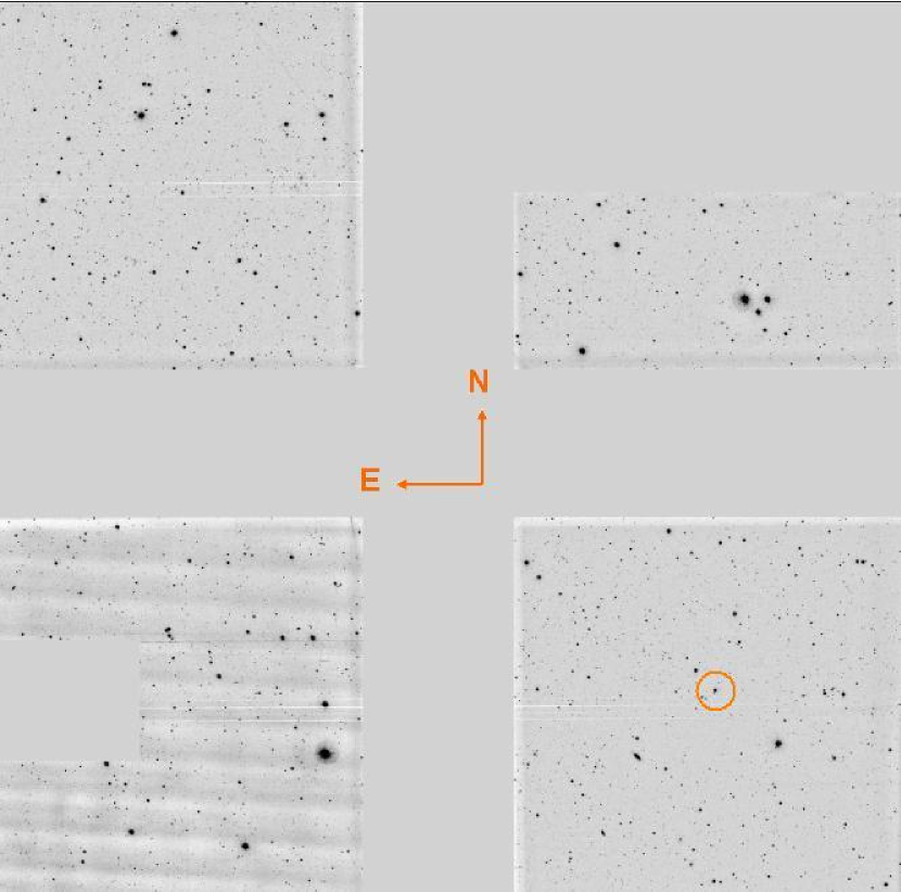
Figure 1.— Example 90Prime data frame. The PG0923+201 field in $u$,$g$ (upper left, right) and $r$,$i$ (lower left,right).

We calculated photometric, Kron, and Petrosian magnitudes using the SExtractor package (Bertin & Arnouts, 1996) on the full exposure-time flux-calibrated co-added images of each filter. We found that optimal source extraction was achieved by considering each amplifier section of each image on a case-by-base basis for amps 1-8 and the extraction parameters used thus vary slightly over the full mosaic. We give a brief summary of those parameter choices here. Amps 1, 2, and 3, are typically low noise and free of bad columns. So we used $1.5\sigma$ for detection and analyze thresholds, DETECT_THRESH and ANALYZE_THRESH. Since the fields are crowded, we use a balanced combination of background and deblending parameters, BACK_SIZE, DEBLEND_NTHRESH, and DEBLEND_MINCONT, to detect as many individual objects and as close as possible to stars or foreground galaxies but to avoid over-resolving. Amp 4 has noise patterns which are enhanced by resampling. To overcome this problem we used a moderately higher detection threshold, $\sim$3, and larger area to estimate the background with deblending parameters set to identify the strips as artificial bright sources. In some extreme cases we mask the noise pattern manually. Amps 5 and 6 have a higher noise level than amps 1 and 2 but typically free of fixed patterns, so we use the same technique as amp 1 but with a higher detection threshold, $\sim$1.7. Amps 7 and 8 behave generally like amps 5 and 6. We dealt with a few cases of noise patterns using the same technique as amp 4, with detection a threshold of $\sim$2.3.

To remove bad columns and bright stars and their associated diffraction patterns, we created image masks which consist of: (1) a manually generated mask for the interchip gaps; (2) a mask for a consistent trap present in chip 3, overlapping amps 5 and 6; (3) a bright star mask created manually by identifying the bright stars in a given frame from the SExtractor output and growing the masked regions using the measured FWHM; (4) a bad pixel mask created using the IRAF task objmasks to mask pixels with pixel values $15\sigma$ below the background; and finally, (5) a bleed trail mask created by using the segmentation map created by SExtractor for a detection threshold $\sim$80-100 and very low debelending parameter and large background estimates, thus including all the bleed patterns. We created masks for each image of each field in every filter individually. The downside of this technique is that step (5) can include some bright foreground galaxies into the mask, so we recover these from careful inspection of the images in all four filters. As an example, our mask frame for PG0923+201 in u filter (Fig. 1) is shown in Fig. 2.

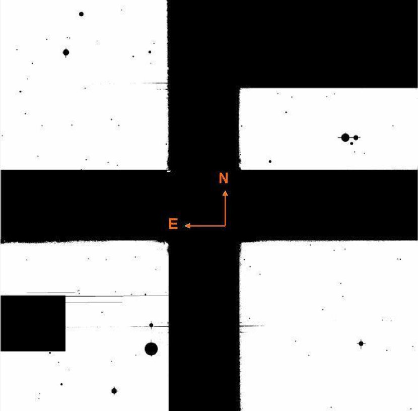
Figure 2.— Example of a frame mask, for the PG0923+201 in u filter, shown in Fig. 1, including inter-chip gaps, trap in amps 5 and 6, bad pixel/columns, and bright stars.

Due to the large dithering of individual frames before co-adding, some regions have lower co-added exposure time than the full stacked image. To decrease the biases on galaxy counting when using a certain detection limit on magnitude, we cut the corners and more from inner-gaps to include only the regions with uniform co-added exposure time in each final image. We also mask objects with centers within 8 pixels of a masked region or an edge from the final catalogs. Finally we filter our catalog sources based on the internal SExtractor flags. Here, we present the catalog of objects detected at 5$\sigma$ or greater in $r$ and at 3$\sigma$ or greater in $u$, $g$ and $i$ in Table 2 as a machine readable table. The magnitudes listed are the SExtractor MAG_BEST values, where the Kron_fact and min_radius parameters governing MAG_AUTO were set to 2.5 and 1.5, respectively. Magnitudes of 99 in this table denote non-detections in the $u$, $g$, or $i$ filter, and values of -99 label objects not observed in one of those filters, primarily due to masking. In the former case, the error bar gives the 1$\sigma$ detection limit for later use with photometric redshift codes. For the analyses discussed in this paper, we use only galaxies detected at $5\sigma$ significance or greater.

Table 290Prime Catalog of Galaxies in Quasar Fields

QSO field	RA	Dec	$u$	$\sigma_{u}$	$g$	$\sigma_{g}$	$r$	$\sigma_{r}$	$i$	$\sigma_{i}$	A	$\sigma_{\rm A}$	B	$\sigma_{\rm B}$	radius	$\theta$	FWHM	class
HS0624p690	98.0779	68.8485	23.10	0.14	99.00	25.52	21.20	0.08	20.65	0.11	1.443	0.109	0.840	0.064	2.56	-12.91	5.05	0.02
HS0624p690	98.1246	68.8445	99.00	27.74	99.00	25.52	22.67	0.18	99.00	25.54	0.677	0.143	0.519	0.110	7.79	-75.60	2.93	0.00
HS0624p690	97.2567	68.8409	99.00	27.74	99.00	25.52	21.93	0.11	21.28	0.16	0.852	0.121	0.531	0.075	5.67	-85.21	2.72	0.61
HS0624p690	98.0474	68.8475	99.00	27.74	99.00	25.52	20.80	0.06	19.90	0.08	1.213	0.080	0.863	0.057	3.97	21.11	2.96	0.96
HS0624p690	97.5498	68.8449	99.00	27.74	99.00	25.52	21.03	0.07	99.00	25.54	0.964	0.069	0.920	0.065	5.46	-35.21	2.37	0.26
HS0624p690	97.6265	68.8442	99.00	27.74	99.00	25.52	22.11	0.13	22.12	0.23	0.799	0.116	0.603	0.088	5.97	61.78	2.45	0.57
HS0624p690	97.4941	68.8537	99.00	27.74	99.00	25.52	21.78	0.11	21.71	0.19	0.981	0.118	0.682	0.082	5.02	-82.06	3.82	0.12
HS0624p690	98.1444	68.8458	99.00	27.74	99.00	25.52	21.85	0.11	20.80	0.12	0.799	0.107	0.562	0.075	5.90	73.74	2.28	0.73
HS0624p690	97.5849	68.8437	99.00	27.74	99.00	25.52	22.75	0.17	22.25	0.24	0.535	0.129	0.432	0.104	6.39	59.89	2.28	0.50
HS0624p690	97.7454	68.8461	99.00	27.74	99.00	25.52	21.79	0.11	20.74	0.12	0.858	0.109	0.740	0.094	5.77	29.80	2.87	0.10
HS0624p690	97.2771	68.8423	99.00	27.74	99.00	25.52	22.81	0.18	99.00	25.54	0.466	0.144	0.402	0.125	8.71	71.16	2.58	0.34
HS0624p690	97.8299	68.8482	99.00	27.74	99.00	25.52	21.17	0.08	20.56	0.11	1.254	0.098	0.846	0.066	3.67	46.78	3.74	0.21
HS0624p690	97.5091	68.8468	99.00	27.74	21.62	0.10	21.40	0.09	21.00	0.14	0.942	0.086	0.733	0.067	4.76	-29.61	2.48	0.86
HS0624p690	97.5560	68.8461	99.00	27.74	99.00	25.52	22.41	0.15	99.00	25.54	0.642	0.111	0.559	0.097	6.31	18.58	2.16	0.64
HS0624p690	98.0133	68.8473	99.00	27.74	99.00	25.52	22.77	0.18	21.12	0.14	0.753	0.166	0.462	0.102	5.87	-88.26	3.53	0.23
HS0624p690	97.3695	68.8452	99.00	27.74	99.00	25.52	22.90	0.18	22.11	0.23	0.704	0.156	0.423	0.094	5.34	75.93	3.26	0.52
HS0624p690	97.3791	68.8490	99.00	27.74	99.00	25.52	20.78	0.06	99.00	25.54	1.245	0.079	0.874	0.055	5.03	28.43	2.92	0.20
HS0624p690	97.9586	68.8496	99.00	27.74	99.00	25.52	22.51	0.16	21.22	0.15	0.571	0.125	0.490	0.107	6.94	75.39	2.82	0.49
HS0624p690	97.5345	68.8568	19.66	0.03	18.32	0.02	17.46	0.01	17.10	0.02	2.327	0.029	2.117	0.027	3.37	-74.43	3.91	0.03
HS0624p690	97.5649	68.8494	99.00	27.74	99.00	25.52	22.12	0.13	21.59	0.18	0.542	0.155	0.378	0.108	8.39	-13.78	2.36	0.36
HS0624p690	97.0202	68.8484	99.00	27.74	99.00	25.52	20.98	0.07	20.17	0.09	1.610	0.121	0.900	0.068	4.66	54.87	4.81	0.39
HS0624p690	97.8307	68.8524	99.00	27.74	99.00	25.52	21.14	0.08	20.04	0.09	0.858	0.065	0.760	0.057	4.07	79.73	2.00	0.96
HS0624p690	97.3351	68.8497	22.32	0.09	99.00	25.52	21.71	0.10	21.37	0.16	0.953	0.101	0.758	0.080	3.94	65.93	3.44	0.08
HS0624p690	98.1068	68.8543	99.00	27.74	20.92	0.07	19.92	0.04	18.59	0.04	1.174	0.047	0.915	0.037	3.56	80.00	2.86	0.94
HS0624p690	97.1526	68.8478	99.00	27.74	99.00	25.52	22.41	0.15	99.00	25.54	0.676	0.147	0.501	0.109	7.64	-77.44	3.48	0.47
HS0624p690	97.9007	68.8552	99.00	27.74	99.00	25.52	20.11	0.05	19.11	0.06	1.381	0.062	0.896	0.040	3.47	9.03	3.23	0.94
HS0624p690	97.7168	68.8546	99.00	27.74	99.00	25.52	20.83	0.07	20.13	0.09	1.116	0.072	0.897	0.058	4.24	-75.39	2.69	0.53
HS0624p690	97.8514	68.8552	99.00	27.74	99.00	25.52	21.59	0.10	21.05	0.14	0.912	0.125	0.780	0.107	6.80	0.23	4.54	0.00
HS0624p690	97.9116	68.8545	99.00	27.74	99.00	25.52	22.63	0.16	21.52	0.17	0.705	0.127	0.522	0.094	4.74	74.68	3.43	0.64
HS0624p690	98.0572	68.8560	22.87	0.13	99.00	25.52	21.29	0.09	20.81	0.12	1.592	0.142	0.783	0.070	4.98	87.82	5.97	0.00
HS0624p690	97.6051	68.8607	99.00	27.74	99.00	25.52	22.02	0.12	22.28	0.24	0.863	0.114	0.664	0.088	5.13	85.51	2.90	0.12

We estimate systematic error and scatter due photometric calibration for all four filters using a final comparison with the SDSS photometry. For this comparison, we use all objects detected in our catalogs at $\geq$5$\sigma$ and with a SExtractor classification parameter (CLASS_STAR, described in the next section) likely to be a galaxy, $<$0.3. We also require the relative error in the SDSS magnitude to be smaller than 1%. The values of the systematic shifts are small, typically less than $0.04$. They are listed in Table 3 and plotted for the $g$ band in Fig. 3. Also in Table 3 we list the 95% confidence on the systematic offset, along with the total photometric statistical uncertainties in each band and their 95% confidence interval. The total statistical uncertainties are obtained from adding the systematic offsets from SDSS in quadrature with the standard deviation of the distribution of SExtractor magnitude errors for each filter. The mean and standard deviation of those distributions are listed separately for each field in Table 4.

Table 3Flux Calibration Errors

filter	Systematic err.	95% conf.	Total	95% conf.
$u$	-0.039	0.011	0.305	0.009
$g$	-0.083	0.006	0.152	0.005
$r$	-0.028	0.008	0.122	0.007
$i$	-0.022	0.013	0.066	0.006

Table 4Individual Flux Calibration Errors

field	filter	Systematic err.	95% conf.	Total	95% conf.
MRK586	$u$	-0.061	0.016	0.328	0.012
MRK586	$g$	-0.026	0.012	0.253	0.010
MRK586	$r$	0.007	0.016	0.139	0.014
PG0844+349	$u$	0.009	0.013	0.293	0.010
PG0844+349	$r$	-0.031	0.008	0.131	0.007
PG0923+201	$u$	0.003	0.013	0.356	0.011
PG0923+201	$g$	-0.062	0.012	0.169	0.011
PG0923+201	$r$	0.022	0.012	0.144	0.010
PG0923+201	$i$	0.119	0.020	0.199	0.016
PG0953+414	$u$	0.005	0.011	0.286	0.009
PG0953+414	$g$	-0.030	0.008	0.134	0.006
PG0953+414	$r$	-0.008	0.010	0.114	0.009
PG0953+414	$i$	0.062	0.013	0.131	0.010
PG1116+215	$u$	-0.019	0.013	0.317	0.010
PG1116+215	$g$	-0.029	0.025	0.118	0.015
PG1116+215	$r$	-0.019	0.041	0.070	0.019
PG1116+215	$i$	0.095	0.018	0.171	0.014
PG1307+085	$u$	0.034	0.010	0.292	0.008
PG1307+085	$g$	-0.046	0.010	0.148	0.008
PG1307+085	$r$	-0.014	0.006	0.071	0.005
PG1307+085	$i$	0.067	0.018	0.145	0.012
PG1404+226	$u$	-0.117	0.016	0.376	0.013
PG1404+226	$g$	-0.076	0.010	0.172	0.008
PG1404+226	$r$	-0.032	0.008	0.134	0.007
PG1404+226	$i$	0.064	0.022	0.171	0.018
PG1444+407	$u$	-0.083	0.014	0.284	0.012
PG1444+407	$g$	-0.089	0.008	0.148	0.007
PG1444+407	$r$	-0.036	0.018	0.111	0.016
PG1444+407	$i$	0.006	0.013	0.145	0.011
PG1545+210	$u$	-0.005	0.007	0.331	0.006
PG1545+210	$g$	-0.091	0.014	0.165	0.013
PG1545+210	$r$	-0.017	0.011	0.093	0.008
PG1545+210	$i$	0.036	0.017	0.161	0.014
PG1612+261	$u$	-0.088	0.014	0.305	0.011
PG1612+261	$g$	-0.110	0.010	0.128	0.008
PG1612+261	$r$	-0.045	0.011	0.108	0.008
PG1612+261	$i$	0.033	0.012	0.185	0.010
Q2141+175	$g$	-0.093	0.010	0.155	0.007
Q2141+175	$r$	-0.058	0.012	0.100	0.011
Q2141+175	$i$	0.010	0.021	0.185	0.014

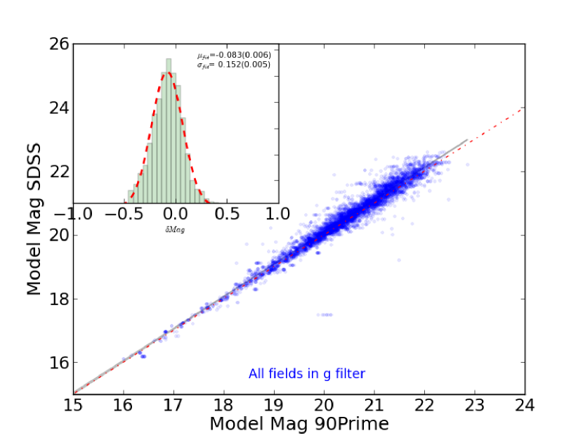
Figure 3.— Example of error estimates from photometric calibration process in g filter from all fields.

2.2.2 Star-Galaxy Separation and Filtering

SExtractor calculates a CLASS_STAR flag based on core geometry of the light distribution of the detected objects, where values near 1 indicate a centrally concentrated star and those near 0 indicate a galaxy. This parameter is sensitive to the value of the input parameter SEEING_FWHM. We measure this input parameter from objects clearly classified as stars ($\rm{CLASS\_STAR}>0.9$) in initial photometric catalogs, which were created from a first pass with SExtractor on the masked images. To improve the accuracy of the CLASS_STAR star-galaxy separation output parameter, we performed this measurement iteratively until we reached convergence between the input value of the SEEING_FWHM and the measured FWHM of the stellar catalog sources. We achieved convergence of $<$0.1″ in 1-2 iterations. In order to determine how to use this CLASS_STAR parameter to best distinguish stars from galaxies in our final catalogs, we performed Monte-Carlo simulations of our data set using synthetic input stars that we then extract from the data frames using the same SExtractor parameters as we used on the data. Using the IRAF task mkobjects, we generated synthetic stars with magnitudes between 15 and 27 and with PSFs that matched those of stellar objects in the post-iteration catalogs. We randomly distributed these synthetic stars on chips 1 and 4 (amps 1,2,7, and 8) of each image, to bracket the best and worst quality CCDs in the mosaic. After extracting these simulated stars, we see the typical behavior of the CLASS_STAR parameter, i. e. that it is a reliable star-galaxy separator at bright magnitudes but at a particular threshold magnitude, CLASS_STAR is spread evenly between 1.0 and some saturation value, 0.35 for our 90Prime frames. Thus, at magnitudes dimmer than the threshold, we cannot rely on this parameter alone to separate galaxies from stars. This threshold magnitude varies across our data frames, but for each frame, we fit a function to the lower envelope of CLASS_STAR versus magnitude, $m$:

$${\rm CLASS\_STAR}=a/(1.0+\exp((m-b)/c))+d$$ (1)

where $m$ is the magnitude in the relevant filter, and $a$, $b$, $c$, and $d$ are fitted parameters. We use the fits to this expression in our final star-galaxy separation algorithm. Figure 4 shows an example of this fitting.

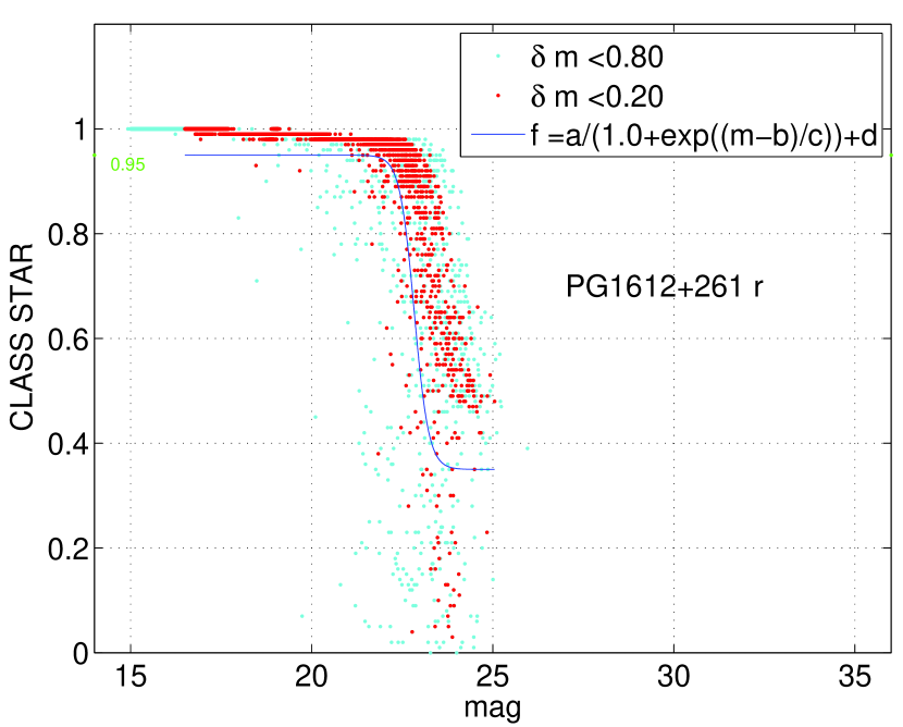
Figure 4.— CLASS_STAR versus r for PG1612+261 with the fit to Equ. 1. Cyan(red) points are points for which the difference between the input and output stellar magnitudes in the Monte-Carlo simulations was less than 0.8(0.2). The fit is designed to find the best inner envelope for the red data reaching asymptotic value of $0.95$ at lowest magnitude.

Equ. 1 is used to define a cut in the CLASS_STAR parameter as function of source magnitude. We find that using this function as a strict cut results in many faint sources lost from our catalogs, so we relax this criterion and rely on a color based criterion as well. To construct the color criterion, we use the unambiguous stellar sources in the matched catalogs, those with CLASS_STAR $>$ 0.95 in all filters, along with the sources in the Gunn-Stryker Atlas (Gunn & Stryker, 1983) to define the stellar locus in color-color space. We then exclude from our catalogs any source that lies within a specified distance from that locus in both $g-r$ versus $u-g$ and $r-i$ versus $g-r$. This distance is allowed to vary in order to give the best match in number counts to our adopted luminosity functions as described below, but it is typically 0.1-0.3. In order to use the color information for sources with only one available color, we use a technique similar to that described by Coil et al. (2004). The binned distributions of the stars in our catalogs in each color, normalized to have a maximum value of unity, are used to assign a probability of being a star, $p_{s}$. Objects having a $p_{s}$ above a threshold value are excluded from the final galaxy catalogs. This threshold is also allowed to vary slightly, typically between 0.7 and 0.8, to get good agreement in the number counts in each filter. The resulting number counts from these final catalogs, shown below, give us confidence in this star-galaxy separation technique. In Figure 5, we show the positions of the 5$\sigma$ galaxies in $u$, $g$, $r$, and $i$ in the portion of the field of PG1444+407 covered by chip 1, along with the position of the quasar itself.

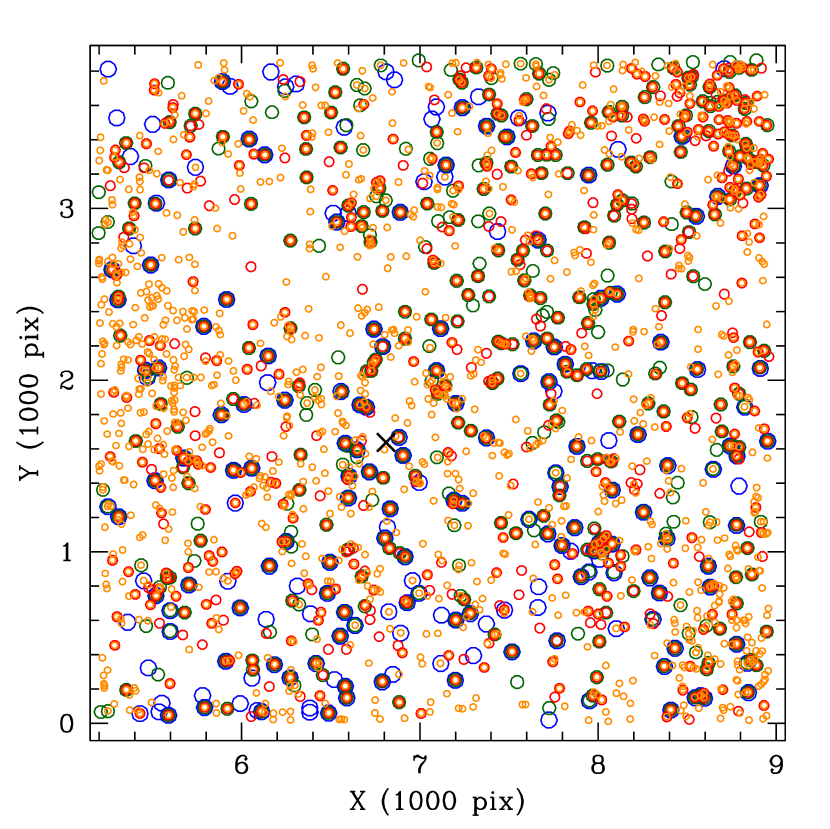
Figure 5.— Blue, green, red, and orange circles show the positions of galaxies detected in $u$, $g$, $r$, and $i$ at $>5\sigma$ significance with magnitude brighter than the limiting magnitude listed in column 3 of Table 5 for chip 1 of the PG1444+407 field. Black cross marks the position of PG1444+407 itself.

2.2.3 Limiting Magnitudes

We characterize the depth of our data frames in two ways: (1) by finding the magnitude at which the lower envelope of the distribution of magnitude errors for stars in the catalogs equals 0.217, or 5$\sigma$ and (2) by using the magnitude distribution of all catalog objects detected at $>4.5\sigma$. We show examples of each in Figures 6 and 7 and tabulate these values for each co-added frame in Table 5. Because we used slightly modified SExtractor parameters for the different amps of the full mosaic, we calculated the limiting magnitudes separately for each amp using method (1). We find that the values for all other amps agree with that of amp 1 to within $<0.03$ magnitudes on average, so we report only values for that amplifier.

Table 5Limiting Magnitudes

QSO	filter	5$\sigma$ mlim	3$\sigma$ mlim	m(complete)
		method (1)	method(1)	method (2)
HS0624+6907	$u$	23.8	23.9	22.9
HS0624+6907	$g$	21.9	21.9	20.7
HS0624+6907	$r$	23.1	23.4	22.1
HS0624+6907	$i$	22.0	23.1	21.7
MRK586	$u$	22.9	24.0	22.5
MRK586	$g$	23.6	24.5	22.9
MRK586	$r$	23.3	24.4	23.1
PG0844+349	$u$	23.9	24.5	23.3
PG0844+349	$r$	24.0	25.1	23.3
PG0923+201	$u$	23.7	24.8	23.5
PG0923+201	$g$	23.6	24.7	23.3
PG0923+201	$r$	22.7	23.8	22.5
PG0923+201	$i$	22.8	24.0	22.3
PG0953+414	$u$	24.1	25.2	23.9
PG0953+414	$g$	22.9	24.1	22.9
PG0953+414	$r$	23.3	24.4	23.1
PG0953+414	$i$	23.6	24.7	22.7
PG1116+215	$u$	23.7	24.8	23.5
PG1116+215	$g$	22.0	23.0	21.7
PG1116+215	$r$	22.2	23.3	22.1
PG1116+215	$i$	22.8	23.9	22.5
PG1307+085	$u$	23.5	24.6	23.3
PG1307+085	$g$	22.7	23.9	22.7
PG1307+085	$r$	23.1	24.2	23.1
PG1307+085	$i$	22.9	24.0	22.7
PG1404+226	$u$	23.6	24.6	23.3
PG1404+226	$g$	23.6	24.8	23.5
PG1404+226	$r$	24.0	25.1	23.5
PG1404+226	$i$	22.8	23.9	22.5
PG1444+407	$u$	23.4	24.6	23.3
PG1444+407	$g$	23.4	24.6	23.3
PG1444+407	$r$	23.2	24.4	23.1
PG1444+407	$i$	22.8	24.0	22.7
PG1545+210	$u$	23.8	24.9	23.5
PG1545+210	$g$	23.5	24.7	23.3
PG1545+210	$r$	23.1	24.2	22.9
PG1545+210	$i$	22.8	23.9	22.3
PG1612+261	$u$	23.3	24.4	23.1
PG1612+261	$g$	23.9	25.0	23.7
PG1612+261	$r$	23.6	24.7	23.5
PG1612+261	$i$	23.1	24.3	22.9
Q2141+175	$g$	23.8	24.9	23.7
Q2141+175	$r$	23.4	24.5	23.3
Q2141+175	$i$	22.6	23.8	22.3

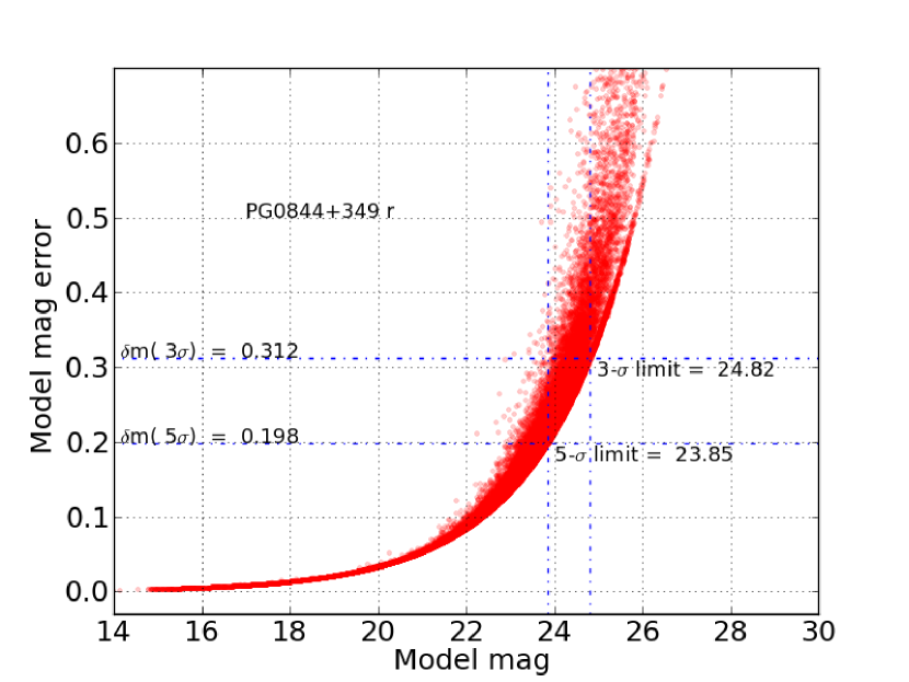
Figure 6.— Example of method (1) for calculating limiting magnitudes at various significance levels.

Figure 7.— Example of method (3) for calculating completeness using the magnitude distribution of all catalog objects detected at $>4.5\sigma$.

We treat method (1) as our estimator of the limiting magnitude at a particular level of significance. Because we use stars only for method (1), it is affected by our ability to recover faint extended galaxies from the images. Method (2) therefore best characterizes the depth of the galaxy catalogs, since those objects dominate the number counts at the faintest magnitudes, assuming our star-galaxy separation technique is robust. We discuss this further below, in Section 3.

Results for each field/filter with each method are listed in Table 5. For reference, the SDSS limiting magnitudes in $(u,g,r,i)$ are (22.0, 22.2, 22.2, 21.3), corresponding to 95% completeness limits. These values may be compared with column 4, where we list the $3\sigma$ limiting magnitudes found via method (1). The stacked $g$ band image of the HS0624+6907 field was created from a combination of data taken on photometric and non-photometric nights, calibrated as described above. The resuling image in this particular field and filter had a resulting level of noise that necessitated a high detection threshold within SExtractor to avoid numerous spurious detections around bright sources. Thus, the 3- and 5$\sigma$ limiting magnitudes are reported here to be the same, as there are no sources extracted at less than 4$\sigma$. This also results in a shallow field compared to the other photometry reported here. Note that the limiting magnitudes in the 90Prime data are significantly fainter than SDSS in most other fields and filters.

3. Number Counts

In Figure 8 we show the galaxy number counts in all four bins from our 90Prime fields, over a total of 7.35, 7.45, 8.95, and 7.03 deg² in $u$, $g$, $r$, and $i$, respectively.

Figure 8.— Number of galaxies in 0.5 magnitude bins per square degree in our 90Prime fields in $u$, $g$, $r$, and $i$. Solid lines are the number counts predicted by the luminosity function in each band. The vertical dotted and dashed lines show the limiting magnitudes for Samples 1 and 2 respectively, listed in Table 6 and discussed in Section 4.

The solid lines in Figure 8 show the predicted number of galaxies for our adopted luminosity functions in each band. Luminosity function parameters adopted are shown in Fig. 9. The curves shown here are polynomial fits to the parameter values derived as a function of redshift from several surveys: in $u$, we adopt the parameters found by Prescott et al. (2009) from the DEEP2 and SDSS $u$-band Galaxy Survey; and for the $r$ band, we adopt the parameters found by Cool et al. (2012) from the AGES survey. For the $g$ band, we adopt the $B$ band values from the DEEP2 survey (Faber et al., 2007), using the $g$ band luminosity function parameter measurements of Loveday et al. (2012) to constrain our fits at $z=0$. We make this choice because: (a) the wavelength coverage of $B$ overlaps that of the SDSS $g$ filter; (b) the agreement between these B band luminosity function parameters and the directly measured parameters in $g$ from Loveday et al. (2012) is good at $z<0.5$; and (c) while no AGN with $z>0.5$ are considered in this work, the Faber et al. (2007) study provides a more robust and convenient way to parametrize the luminosity function to redshifts beyond $z=0.5$ than an extrapolation of the Loveday et al. (2012) measurements, enabling us to estimate the numbers of background galaxies reliably. For the $i$ band, we adopt a modification of the evolution derived by Loveday et al. (2012). The $M^{*}$ follows the parametric solution found by these authors, but we fix its value at $z>0.6$ to the $z=0.6$ value. For $\phi^{*}$, we find good agreement with our galaxy number counts by using the Loveday et al. (2012) value at $z=0$ and adopting the redshift evolution for the $r$ band, noting that the Loveday et al. (2012) parametrized solution found no redshift evolution in this band. The $M^{*}$ and $\phi^{*}$ evolution in $i$ found by Loveday et al. (2012) and extrapolated to $z>0.5$ is shown in Fig. 9. For $\alpha$, the values from these various studies are (-1.0, -1.3, -1.05, -1.12) for $(u,B,r,i)$. We extrapolate the highest redshift values from each study to all higher redshifts for our calculations, although at the depths of our survey, we are generally not sensitive to galaxies with $z\gtrsim 1.5$.

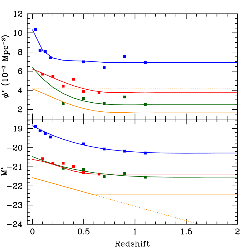
Figure 9.— Polynomial fits (solid curves) to luminosity function parameter values $\phi^{*}$ and $M^{*}$ (squares) from Prescott et al. (2009) ($u$ band, blue), (Faber et al., 2007) ($B$ band, green), Cool et al. (2012) ($r$ band, red), and For $i$ band (orange) the Loveday et al. (2012) parametrized model for $M^{*}$ is set at the $z=0.6$ value for larger redshifts, and for $\phi^{*}$ it follows the redshift evolution of the $r$ band from its $z=0$ value. Dashed curves show Loveday et al. (2012) parametrized models for the redshift evolution of each parameter in $i$ extrapolated to $z>0.5$.

4. Correlation Functions

To examine the galaxy autocorrelation function and the galaxy-quasar cross-correlation signal in the 90Prime fields, we use a chip-by-chip approach to the calculations. Due to the large interchip gaps in the 90Prime mosaic, the masked region in chip 3, and the often masked amplifier 4 on chip 2 (see Fig. 2), the correlation functions described below contain significant structure when calculated at scales that span these regions, even with a large simulated set of random points. To verify this, we performed a series of simulations with 5000 random data points created with regions identical to those in the real data. With the random data, we expect zero correlation but find that there is significant structure in the correlation function when the masks are applied, and so we calculate the correlation functions in the real data on scales that minimize the effect of the masks introducing structure into the correlation functions that is unrelated to the galaxy distributions.

To perform the correlation function calculations to a uniform depth, we confine galaxy magnitudes to the limit defined by the shallowest field in the sample. These depths are listed in Table 6 for the two cases we consider: Sample 1 is the sample of all quasar fields with the HS0624+6901 $g$ band excluded due to its shallow depth ($g=21.79$) and Sample 2 is a sample of deeper fields, constructed by leaving out other shallow fields in each filter to achieve the depth listed in Table 6. The Sample 1 and 2 limiting magnitudes are also shown as vertical dotted and dashed lines in Figure 8. In our calculations, we will consider other AGN in the primary sample fields with redshifts up to $z=0.5$. Thus, in Table 6 we also list the absolute magnitudes relative to M^∗ reached for $z=0.5$ galaxies in Samples 1 and 2 in order to demonstrate the coverage of the galaxy luminosity function at the redshifts of the AGN in the overall sample.

Table 6Sample Limiting Magnitudes

Filter	mlim	Mlim - M∗
Sample 1
$u$	22.82	-1.1
$g$	21.95	-0.8
$r$	22.14	0.3
$i$	22.06	1.6
Sample 2
$u$	23.31	-0.6
$g$	22.92	0.2
$r$	23.01	1.1
$i$	22.81	2.3

4.1. Galaxy-Galaxy Clustering

We calculate the angular correlation function of the galaxy-galaxy sample,

$$\omega(\theta)_{\rm true}=A_{\rm gg}\theta^{(1-\gamma)}$$ (2)

using the estimator of Landy & Szalay (1993):

$$\omega(\theta)_{\rm obs}=\frac{N_{\rm gg}(\theta)-2N_{\rm gr}(\theta)-N_{\rm rr}(\theta)}{N_{\rm rr}(\theta)}$$ (3)

where $N_{\rm gg}$ and $N_{\rm rr}$ are the pairwise distances between all galaxies in the sample and all random positions in the survey area at a given angular separation, $\theta$, normalized by the total numbers of galaxy-galaxy and random-random pairwise distances. The $N_{\rm gr}$ term is the normalized number of pairwise distances between all galaxies and random points in each $\theta$ bin.

The random points are generated by Monte Carlo simulations which place galaxies at random positions within the areas covered by the 90Prime images. These catalogs of random positions are masked in the same way as the galaxy catalogs. We generated 10 realizations of each field in each filter, with $\sim$40,000 points in each realization. The Poisson error in each bin is given by

$$\Delta\omega(\theta)=\frac{1+\omega(\theta)}{\sqrt{N_{\rm gg}(\theta)}}.$$ (4)

This estimator of the angular correlation function must be corrected for the integral constraint, which requires the function to reach zero at the survey edges, so that

$$\omega(\theta)_{\rm true}=\omega(\theta)_{\rm obs}+C$$ (5)

where

$$C=\frac{1}{\Omega^{2}}\int\int\omega(\theta)d\Omega d\Omega=\frac{\sum N_{\rm rr}(\theta)A_{\rm gg}\theta^{(1-\gamma)}}{\sum N_{\rm rr}(\theta)}$$ (6)

(Groth & Peebles, 1977; Infante, 1994).

In each filter, we solve for A_gg and $\gamma$ independently using a least squares technique and derive the uncertainties in the parameters by finding the values of each that yield $\chi^{2}_{\rm min}+1$.

4.2. Galaxy-Quasar Clustering

For galaxy-quasar clustering, the autocorrelation function does not apply, so we follow Croom & Shanks (1999) and Brown et al. (2001)

$$\omega(\theta)_{\rm true}=\omega(\theta)_{\rm obs}+C=\frac{N_{\rm gq}(\theta)}{N_{\rm qr}(\theta)}-1+C$$ (7)

where $N_{\rm gq}$ and $N_{\rm qr}$ are the numbers of galaxy-quasar and quasar-random pairs at each value of $\theta$, normalized by the numbers of galaxies and random points respectively and $C$ is defined as in Equ. 6.

Here we solve for A_gq for a fixed value of $\gamma$ and again derive the uncertainties in the parameters by finding the values of each that yield $\chi^{2}_{\rm min}+1$.

4.2.1 Correlation Length

The galaxy-galaxy and the galaxy-quasar angular correlation functions can be used to derive the correlation length, $r_{0}$, of the spatial correlation function

$$\xi=\left(\frac{r}{r_{0}}\right)^{\gamma}(1+z)^{-(3+\epsilon)}$$ (8)

for galaxy-galaxy and galaxy-quasar clustering using Limber’s equation (Limber, 1953), which relates $r_{0}$ to the amplitude of the angular correlation function given in Equation 2:

$$A=kr_{0}^{\gamma}\frac{\int_{0}^{\infty}F(z)D_{\theta}^{(1-\gamma)}(z)N_{x}(z)N_{g}(z)g(z)dz}{\int_{0}^{\infty}N_{x}(z)N_{g}(z)dz}$$ (9)

where

$$k=\sqrt{(}\pi)\frac{\Gamma\left(\frac{\gamma-1}{2}\right)}{\Gamma\left(\frac{\gamma}{2}\right)}$$ (10)

and $F(z)$ describes the redshift evolution of the correlation function in Equ. 8 with $\epsilon=0$ or $\gamma-3$ for clustering fixed in physical or comoving coordinates, or $\epsilon=\gamma-1$ for clustering according to linear theory. Finally,

$$g(z)=\frac{H_{0}}{c}[(1+z)^{3}(1+\Omega_{m}z+\Omega_{\Lambda}((1+z)^{-2}-1)^{\frac{1}{2}}]$$ (11)

and $N_{x}$ corresponds to either $N_{g}$ or $N_{q}$ depending on whether we are considering galaxy-galaxy or galaxy-quasar clustering.

The redshift distribution of the galaxies in our 90Prime Samples 1 and 2, calculated from the Schechter luminosity function parameters shown in Figure 9 and the magnitude limits determined by the values listed in Table 6 in each of the four bands is shown in Figure 10.

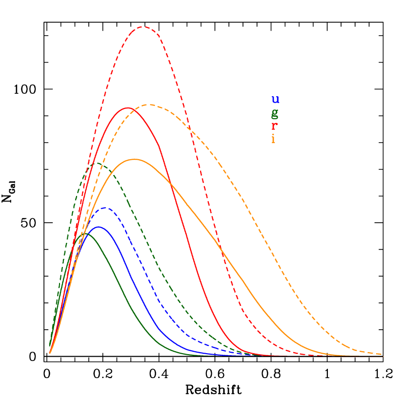
Figure 10.— Number of galaxies in $u$, $g$, $r$, $i$ frames in all 90Prime fields from integration of a Schechter luminosity function with parameters as shown in Figure 9, integrated to the limiting magnitudes listed in column 3 of Table 5. Solid lines show Sample 1 and dashed lines represent Sample 2.

4.2.2 Correlation Amplitude

We also calculate the amplitude of the galaxy-quasar correlation function, B_gq using the technique described by Ellingson et al. (1991), Finn et al. (2001), McLure & Dunlop (2001b), and recently by Ramos Almeida et al. (2013). We first begin with the angular correlation function, which describes the clustering of galaxies about some particular object using the following relation:

$$n(\theta)d\Omega=N_{g}[1+w(\theta)]d\Omega.$$ (12)

Here, $n(\theta)d\Omega$ represents the number of galaxies within a solid angle d$\Omega$ at an angular distance $\theta$ from the object. The term $N_{g}$ represents the average galaxy surface density, and $w(\theta)=A_{gq}\theta^{1-\gamma}$ represents the angular cross-correlation function discussed above. To calculate B_gq, we first determine the amplitude, A_gq, from the integral of the angular correlation function within a fixed angular radius, $\theta$,

$$A_{gq}=\frac{N_{t}-N_{b}}{N_{b}}\frac{(3-\gamma)}{2}\theta^{\gamma-1},$$ (13)

where $N_{t}$ represents the quasar field galaxy counts, and $N_{b}$ represents the background galaxy counts both within angular distance $\theta$ of the quasar. For each quasar field, we count the galaxies within a specified radius around the quasar, down to the magnitude limit specified by the amplifiers on the chip, $m_{\rm lim}$. To construct the control fields, we use all other regions of the mosaic of the reference quasar as well as any non-quasar regions of the images of our other quasar fields. We place grids of overlapping control fields with the same radius as our reference quasar in each of these regions and count the galaxies brighter than $m_{\rm lim}$. The galaxy counts in these regions may be affected by other galaxy clusters and large scale structures in the quasar fields. We discuss these in detail for each quasar field in Appendix A. To mitigate this problem we take a median of all the counts from these regions and use this as our value for $N_{b}$.

The angular covariance amplitude, A_gq, quantifies any excess in galaxy counts within the quasar field as compared with the background counts of the control field. To de-project the angular cross-correlation function into its spatial equivalent, we use:

$$n(r)dV=\rho_{g}[1+\xi(r)]dV,$$ (14)

where $n(r)$ and $\rho_{g}$ represent the total and expected average galaxy counts within volume $dV$, respectively, and the spatial cross-correlation function, $\xi(r)$, is defined as in Equ. 8, with amplitude B_gq:

$$\xi(r)={\rm B}_{gq}r^{-\gamma},$$ (15)

where $\gamma=1.77$ (Groth & Peebles, 1977). B_gq can be obtained using the following equation relating the spatial clustering amplitude to the angular clustering amplitude (Longair & Seldner, 1979):

$${\rm B}_{gq}=\frac{N_{g}A_{gq}}{\Phi(m_{\rm lim},z)I_{\gamma}}\left[\frac{D}{1+z}\right]^{\gamma-3}.$$ (16)

Here, $D$ is the angular diameter distance to the quasar, and $\phi(z)$ is the galaxy luminosity function integrated to the limiting absolute magnitude of the data at the quasar redshift. The quantity $I_{\gamma}$ is a constant of integration equivalent to $\frac{2^{\gamma}}{(\gamma-1)}\frac{\Gamma(\gamma+1/2)}{\Gamma(\gamma)}$.

The errors in A_gq and B_gq can be calculated using the following equations:

$$\frac{\Delta A_{gq}}{A_{gq}}=\frac{\Delta B_{gq}}{B_{gq}}=\frac{1}{N_{t}-N_{b}}\left[(N_{t}-N_{b})+1.3^{2}N_{b}\right]^{\frac{1}{2}}.$$ (17)

(Yee & López-Cruz, 1999). We normalize the galaxy counts using the luminosity function calculated with the redshift-dependent parameters shown in Fig. 9.

To calculate the predicted average galaxy background counts, $N_{g}$, we integrate the luminosity function using the same redshift-dependent parameters:

$$N_{g}=\int_{0}^{z}\int_{-\infty}^{M_{\rm lim}}\Phi(m,z)\,dmdz$$ (18)

to the relevant luminosity dictated by the limiting magnitude of the data at each redshift. In calculating each value of $M_{\rm lim}$, we apply a median K-correction for galaxies in each filter at each redshift calculated from the KCORRECT code (Blanton & Roweis, 2007) and using the galaxy templates of Kinney et al. (1996).

In our data sample, we adjust the galaxy magnitudes for extinction using galaxy extinction E(B-V) values acquired from the NASA/IPAC Infrared Science Archive for each quasar, and assuming $R_{V}=3.1$ and the reddening curve of O’Donnell (1994). In our calculations, we used a radius of 0.5 $h^{-1}$ Mpc around the sample quasars and for the control fields derived from the other 90Prime images of comparable depth in the same filter, and we fix the parameter $\gamma$ to be 1.77. We follow Finn et al. (2001) and McLure & Dunlop (2001b) in using only galaxies in the range m*-1 - m*+2 in order to eliminate many galaxies in the foreground or background of the quasar of interest.

5. Results

5.1. Comparisons with other work

5.1.1 Correlation Amplitude

Results of the calculations of B_gq are listed in Table 7 and plotted versus quasar redshift in Figure 11, along with values for some of our fields present in the literature. We do not include a value for PG0844+349, as its low redshift, $z=0.064$, results in an angular radius corresponding to 0.5 $h^{-1}$ Mpc that is larger than our contiguous chip areas. We do include this object in our discussion of the angular correlation function below. We also omit the $i$ band data of Q2141+175 from both this calculation and the correlation function calculations as the quasar was placed in amp 4, which was masked due to noise.

The limiting magnitudes of the galaxies included in these calculations are those listed in Table 5 with the exception of PG0953+414 $u$ and $i$ bands (23.7 and 23.2, respectively), PG1404+226 $i$ (22.5), and PG1612+261 $g$ (23.5), as there were no galaxies found in the control fields in these bands down to the quoted magnitude limits. This change in the magnitude limits had no effect on $N_{t}$, the quasar field galaxy counts, but simply increased $N_{b}$, the median number of background galaxies found in the control fields to a number greater than zero, resulting in a finite value of B_gq. No significant differences in the B_gq values were found when imposing a uniform magnitude limit on all the fields, so we opt for using the individual values for each field. All B_gq values are quoted in units of Mpc^γ, where $\gamma=1.77$ unless otherwise noted. The mean values of B_gq we find in ($u$, $g$, $r$, $i$) are (21$\pm$20, 161$\pm$96, 58$\pm$100, and 445$\pm$271).

Given the well-known morphology-density relation (Dressler, 1980) and the fact that radio loud quasars are more commonly found in massive early-type hosts (Hamilton et al., 2002; Best et al., 2005), it may be expected that galaxies cluster more strongly around radio loud quasars than around radio quiet objects. Optical and X-ray selected AGN show no tendency to reside in galaxy group environments (Coldwell & Lambas, 2003; Silverman et al., 2009) but Wold et al. (2001) find that radio loud quasars do prefer group or Abell class 0 environments. Some other studies have found this distinction between the environments of radio loud and radio quiet quasars (Ellingson et al., 1991; Best et al., 2005; Shen et al., 2009; Hickox et al., 2009; Ramos Almeida et al., 2013) while others have not (Fisher et al., 1996; McLure & Dunlop, 2001b; Finn et al., 2001; Wold et al., 2001; Coldwell et al., 2002). As we have only 2 radio loud quasars in our sample, we have little leverage to address this question. However, excluding the two radio loud objects in our sample, PG1545+210 and Q2141+175, we find a systematic decrease in all four filters: $<$ B_gq$>=$ (9$\pm$18, 144$\pm$114, -39$\pm$56, 295$\pm$260). Removing the two additional $u$ fields (PG1444+407 and HS0624+690) and one $g$ field (HS0624+690) that do not have limiting magnitudes that reach M^∗+2 at the redshifts of the AGN does not affect these means significantly, bringing them to 32$\pm$14 and 202$\pm$113 respectively. The error bars reflect the standard deviation in the measurements among all fields in each filter. The median redshift of our sample AGN is 0.18 and the median M_r is -23.7. These modified B_gq averages are all consistent with the galaxy-galaxy correlation amplitude, 20 ($h^{-1}$Mpc)^1.77 (Davis & Peebles, 1983), although within the uncertainties, the average values in $g$ and $i$ are also consistent with richer environments, as discussed in more detail for individual fields below.

Finn et al. (2001) used images of quasar fields taken with the F606W, F675W, and F702W filters and the 2.5′ field of view of the Wide Field Planetary Camera 2 on the Hubble Space Telescope and, scaling to our assumed value of H₀, find $<$B_gq$>=104\pm 22$, $-33\pm 27$, and $133\pm 44$ in those respective filters for radio quiet quasars at median redshifts of 0.17, 0.42 and 0.4. McLure & Dunlop (2001b) find $<$B_gq$>=326\pm 94$ for their sample of radio quiet objects with median redshift of 0.16, also derived from F606W and F675W HST/WFPC2 images. Their dataset is a superset of that of Fisher et al. (1996) who found $<$B_gq$>=132\pm 37$. These HST studies were limited to radii of $\sim$200 kpc, while ground-based studies typically extend to the same 0.5 $h^{-1}$ Mpc scale as ours does. The ground-based V, R, and I photometry of Wold et al. (2001) targets AGN at higher redshift than our AGN sample, $z_{\rm med}=0.714$, and they find $<$B_gq$>=210\pm 82$ for radio quiet quasars. All of these studies show average B_gq values that are larger than B_gg at the $2-3\sigma$ level. Our overall results are more in line with the earlier studies of Smith et al. (1995) and Ellingson et al. (1991), both with $z_{\rm med}\sim 0.4$ who found average B_gq values consistent with B_gg for radio quiet objects.

Table 7B_gq Measurements

QSO	Bgq (Mpcγ)	Filter	Ref.
MRK586	-3$\pm$6	$u$	1
	-36$\pm$137	$g$	1
	0	$r$	1
	93$\pm$161	F606W	2
	13$\pm$82	F606W	3
HS0624+6907	-66$\pm$52	$u$	1
	-319$\pm$279	$g$	1
	-144$\pm$127	$r$	1
	-126$\pm$151	$i$	1
PG0923+201	-76$\pm$25	$u$	1
	-114$\pm$133	$g$	1
	-377$\pm$130	$r$	1
	-529$\pm$291	$i$	1
	500$\pm$269	F675W	2
	119$\pm$81	F606W	3
PG0953+414	30$\pm$28	$u$	1
	207$\pm$101	$g$	1
	-36$\pm$191	$r$	1
	629$\pm$519	$i$	1
	730$\pm$297	F675W	2
	159$\pm$81	F606W	3
PG1116+215	68$\pm$41	$u$	1
	-41$\pm$57	$g$	1
	186$\pm$134	$r$	1
	863$\pm$461	$i$	1
	321$\pm$235	F606W	2
	185$\pm$81	F606W	3
PG1307+085	10$\pm$27	$u$	1
	259$\pm$120	$g$	1
	125$\pm$306	$r$	1
	1461$\pm$778	$i$	1
	112$\pm$176	F606W	2
	170$\pm$82	F606W	3
PG1404+226	85$\pm$85	$u$	1
	942$\pm$522	$g$	1
	143$\pm$759	$r$	1
	707$\pm$854	$i$	1
PG1444+407	-27$\pm$19	$u$	1
	46$\pm$119	$g$	1
	-135$\pm$161	$r$	1
	292$\pm$334	$i$	1
	57$\pm$130	F606W	2
	49$\pm$79	F606W	3
PG1545+210	133$\pm$38	$u$	1
	104$\pm$120	$g$	1
	0	$r$	1
	1643$\pm$404	$i$	1
	206$\pm$199	F606W	2
	242$\pm$79	F606W	3
	236$\pm$120	$r$	4
PG1612+261	56$\pm$27	$u$	1
	354$\pm$237	$g$	1
	-116$\pm$397	$r$	1
	-935$\pm$727	$i$	1
Q2141+175	370$\pm$221	$g$	1
	991$\pm$355	$r$	1
	112$\pm$169	F675W	2

Figure 11.— B_gqversus quasar redshift for all filters. Points have been offset slightly in z for clarity. Black points show values from the literature listed in Table 7. Dotted lines, bottom to top, mark the B_gq values for Abell classes 0-4 (Yee & López-Cruz, 1999) and the dashed line marks the galaxy-galaxy correlation value from Davis & Peebles (1983).

Considering the individual values, we find that there can be a large range of B_gq values obtained for the same field depending on the filter used. Typically, the values of B_gq in the $i$ band tend to be larger than those of the other bands and those calculated in the $u$ band are nearly all consistent with B_gg. As above, for the $r$ band, we compare our individual results with those found in the literature, from Finn et al. (2001) and McLure & Dunlop (2001b), and for PG1545+210, we compare with Yee & Green (1984), who calculated B_gq from $r$ band images taken with the SIT-vidicon camera and the 1.52 m Palomar telescope. We scaled these literature B_gq values for our value of H₀ but otherwise do not correct for different cosmologies used in these other works (McLure & Dunlop (2001b): $H_{0}=50$ km s^-1 Mpc^-1; Finn et al. (2001) $H_{0}=100$ km s^-1 Mpc^-1, both use $\Omega_{\rm m}=1$, $\Omega_{\Lambda}=0$). In most cases our results are consistent with these previous studies. We give a more detailed discussion of these comparisons for each field in Appendix A.

Yee & Ellingson (1993) considered B_gq$>500$ to be a rich cluster environment, and clusters with Abell classes 0, 1 and 2 show values of $\sim$350, $\sim$650, and $\sim$950 respectively, according to Yates et al. (1989). McLure & Dunlop (2001b) suggest a classification based on that of Yee & López-Cruz (1999), where B_gq=(300,700,1100,1500,1900,2300) corresponds to Abell class (0,1,2,3,4,5) respectively. Given the large statistical uncertainties in the B_gq values, we find results marginally greater than 500 in only a few cases, for PG1307+085 and PG1545+210 in the $i$ band, 1461$\pm$778 and 1643$\pm$404, respectively, for PG1404+226 in the $g$ band, 942$\pm$522, and for Q2141+175 in the r band, 991$\pm$355. The radio loud AGN PG1545+210 is known to reside in an Abell class 1 environment (Oemler et al., 1972), though our $i$ band B_gq value is consistent with Abell class 3. The B_gq values for this field in $g$ and $r$ are consistent with B_gg, and in $u$ we find only 133$\pm$38, which is significantly larger than B_gg, but far smaller than the $i$ band value. PG1307+085 has a foreground galaxy cluster in its field at a close projected separation from the quasar and with a similar redshift, $z_{\rm clus}=0.14$ versus $z_{q}=0.155$; and PG1404+226 has a background cluster within the 13.1′ radius corresponding to 0.5 $h^{-1}$ Mpc. Q2141+175 is the only other radio loud AGN in our sample and while it has no known cluster at its redshift or in projection, it is a less well-studied field than many of the others. Thus the B_gq for these other fields may be influenced by foreground, background, or even proximate galaxy clusters, but only in select bands.

There are a handful of other fields that show a significant, positive signal in B_gq in one or more bands, and these are discussed in Appendix A. One field, PG0923+201, shows negative values of B_gq in all bands, with two ($u,r$) at $>2\sigma$. As we discuss in Appendix A, this well-studied field has a compact group consistent with the redshift of the AGN and with a center only 23 $h^{-1}$ kpc from the position of the AGN, making this result an intriguing one. Three other fields, HS0624+690, MRK586, and PG1444+407 show B_gq values in all filters that are either consistent with or significantly less than B_gg. HS0624+690 is the only quasar in our sample, and with $z=0.370$, our limiting magnitudes in $u$ and $g$ allow us to reach only $\sim M^{*}+0.7$ and $\sim M^{*}+0.1$, respectively.

Two other AGN in our sample, PG1116+215 and PG1612+261 lie near galaxy clusters, though their redshifts and position on the sky place them near the peripheries of those clusters. The B_gq values for these fields give no indication of a cluster association: for PG1116+215, all the B_gq values are consistent with B_gg, except the anomalously high value we find for the $i$ band, 863$\pm$461. For PG1612+261, the only filter showing a B_gq marginally larger than B_gg is the $g$ band, for which we find 354$\pm$237, Abell class 0.

5.1.2 Correlation Functions

We show the results for the normalization, $A_{\rm gg}$, and slope, $\gamma$ of the galaxy autocorrelation function in Figure 12 and list the results in Table 8. These calculations were performed for Sample 2. For the $u$ and $g$ filters, we use only chips 1 and 4 as chips 2 and 3 added extra structure due to masking. The $r$ and $i$ filters typically are less affected by this. The use of all chips for $u$ and $g$ gives similar results, but a poorer fit to the form of the autocorrelation function. We avoid separations less than 10″ to mitigate against blending, and because we are restricted to single chips, we calculate the correlation function to a maximum separation of  10′. The errors on the parameters are derived from the variance in that parameter from 100 jackknife samples of the dataset, where the sampling with replacement was done one field/filter at a time.

Table 8Galaxy-Galaxy Clustering Clustering in 90Prime QSO fields

Filter	$\gamma$	$A_{\rm gg}$	$\chi_{\nu}$
$u$	1.51$\pm$0.02	0.13$\pm$0.05	2.9
$g$	1.50$\pm$0.03	0.26$\pm$0.08	10.9
$r$	1.59$\pm$0.03	0.18$\pm$0.04	12.5
$i$	1.53$\pm$0.02	0.18$\pm$0.03	27.1

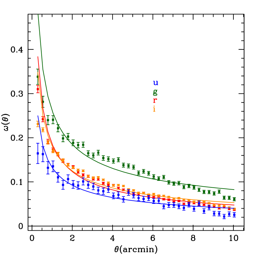
Figure 12.— Galaxy-galaxy angular correlation function in $u,g,r,i$ filters for 90Prime fields.

In our calculations of the galaxy-quasar cross-correlations, we consider quasars in 90Prime fields other than the target quasars themselves, as any clustering may also be present for these objects as well. As discussed above, the galaxy counts in our images are very sparse at $z>1$ and so galaxies associated with clusters, groups, or quasars at these redshifts are generally not of concern to us here. AGN with $z<0.5$ found in the 90Prime frames are listed in Table 9 and the resulting quasar redshift distributions in each filter are shown in Figure 13. The absolute magnitudes relative to M^∗ reached for $z=0.5$ galaxies in Samples 1 and 2 are listed in Table 6.

Table 9Other $z<0.5$ Quasars in 90Prime Fields

QSO	z	Filters
PG0844+349
SDSS J084731.77+351416.4	0.237	$u,r$
2MASX J08503620+3455231	0.144	$u,r$
PG0923+201
SDSS J092507.72+203540.9	0.472	$g,i,r$
SDSS J092525.16+202139.0	0.460	$u,g,r$
SDSS J092536.08+201649.5	0.228	$g$
PG1307+085
Q87GBBWE91 1307+0843	$\cdots$	$r,i$
SDSS J131155.76+085340.9	0.469	$u,g,r,i$
PG1444+407
SDSS J144618.08+412003.0	0.268	$u,g,r,i$
PG1545+210
SDSS J154749.70+205056.5	0.265	$u,g,r$
SDSS J154750.71+210351.1	0.296	$u,g,r$
SDSS J155014.81+212431.5	0.479	$r$
SDSS J155046.30+205803.1	0.401	$u,g,r,i$
2MASS J15505930+2128088	0.372	$u,r$
PG1612+261
HB89 1612+266	0.395	$u,g,r,i$

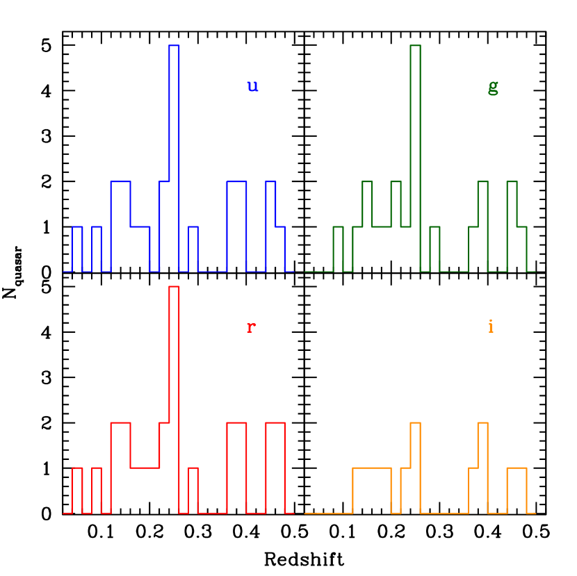
Figure 13.— Redshift distributions of all quasars in the 90Prime fields

We list the results for the normalization A_gq of the galaxy-quasar cross-correlation function in Table 10 for both Samples 1 and 2, where the latter correspond to deeper magnitude limits and fainter galaxy samples. For these solutions, we hold the slope $\gamma$ to be constant at 1.8, the commonly accepted value and 1.5, corresponding to the slope we found from the 90Prime data for the galaxy-galaxy clustering on 10′ scales. This difference in slope changes the normalization at only the $\sim 1\sigma$ level. The results for both slopes are plotted in Figure 14.

Table 10Galaxy-Quasar Clustering in 90Prime QSO fields

Filter	$A_{\rm gq}$	$\chi_{\nu}$	r0 h-1 Mpc
Sample 1, $\gamma=1.8$
$u$	0.49${}^{+0.15}_{-0.14}$	0.39	8.07
$g$	0.23${}^{+0.16}_{-0.14}$	0.69	5.36
$r$	0.21${}^{+0.08}_{-0.07}$	0.70	6.11
$i$	-0.03$\pm 0.07$	1.66	$\cdots$
Sample 1, $\gamma=1.5$
$u$	0.61${}^{+0.21}_{-0.19}$	0.38	16.9
$g$	0.34${}^{+0.22}_{-0.19}$	0.65	11.64
$r$	0.28$\pm$0.10	0.65	12.3
$i$	-0.0027${}^{+0.10}_{-0.09}$	1.68	$\cdots$
Sample 2, $\gamma=1.8$
$u$	0.40${}^{+0.12}_{-0.11}$	0.61	7.76
$g$	-0.04$\pm$0.09	1.03	$\cdots$
$r$	-0.05$\pm$0.05	1.57	$\cdots$
$i$	0.004$\pm$0.05	1.44	0.90
Sample 2, $\gamma=1.5$
$u$	0.51${}^{+0.16}_{-0.15}$	0.57	16.2
$g$	-0.03${}^{+0.12}_{-0.11}$	1.04	$\cdots$
$r$	-0.06${}^{+0.07}_{-0.06}$	1.58	$\cdots$
$i$	0.02$\pm$0.07	1.44	2.95

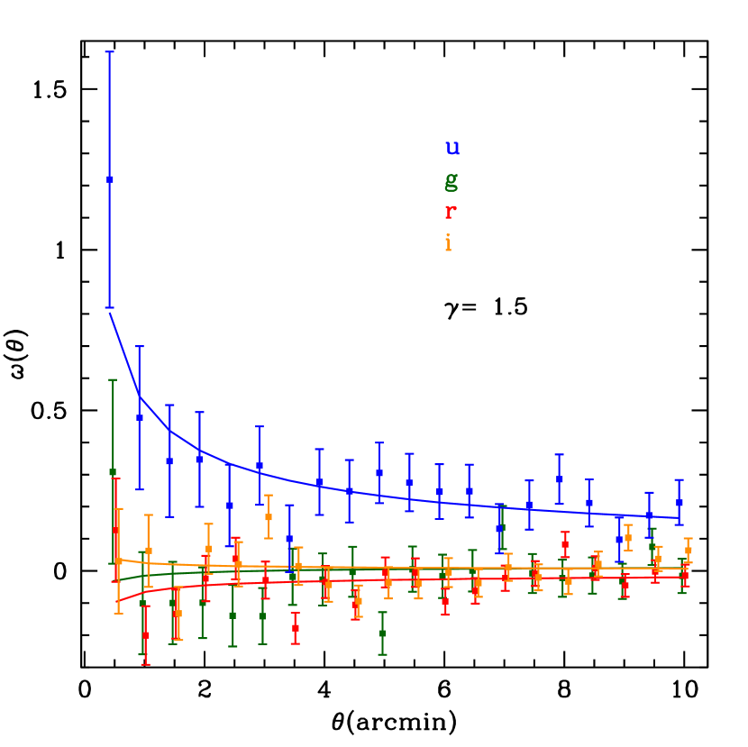
Figure 14.— Quasar-galaxy angular correlation functions in $u,g,r,i$ filters for 90Prime fields for $\gamma=1.8$ and $\gamma=1.5$. Points are offset in x and g fit curve is offset in y by +0.02 for clarity.

Croom & Shanks (1999) found no galaxy-quasar correlation in their sample of $\sim$150 optically and X-ray selected quasars with $z=1-1.5$ and $b_{J}<23$ galaxies in five deep AAT plate fields. In fact, their data showed a weak anti-correlation between these two populations. At the the lower redshifts of our sample, we see significant correlations only in the $u$ band. For Sample 1, there is also a significant positive correlation on the $r$ band, but this does not hold with the inclusion of fainter galaxies in Sample 2. In fact in all bands except the $i$ band, the correlation is significantly smaller for Sample 2, and we also see weak anti-correlations in several cases. In $i$, the normalizations are all consistent with zero for both Samples 1 and 2.

In Table 10, we also tabulate the correlation length for galaxy-quasar clustering, $r_{0}$, found from Limber’s equation, Equation 9, and the galaxy and quasar redshift distributions plotted in Figures 10 and 13. This is undefined for negative values of A_gq, so no correlation length values are reported in Table 10 in these cases. The values we find range from 0.9 $h^{-1}$ Mpc for Sample 2 in the $i$ band with $\gamma=1.8$ to $\sim$16 $h^{-1}$ Mpc for both Samples 1 and 2 in the $u$ band with $\gamma=1.5$. These results are generally within the range found for $0.7<z<1.4$ quasars in the DEEP2 survey by Coil et al. (2007), 0.1 $h^{-1}$ $\lesssim r_{0}\lesssim$ 10 $h^{-1}$ Mpc. Brown et al. (2001) studied a population of galaxy fields around a sample of moderate redshift quasars with $z=0.2-0.7$ and also find a weak correlation, though a stronger one for red galaxies ($r_{0}\sim 7$ $h^{-1}$ Mpc, $\gamma\sim 1.9$) than for blue galaxies ($r_{0}\lesssim 4$ $h^{-1}$ Mpc). These authors provide a summary of results to that time in their Table 1. The value of the correlation length ranges from $\sim$5-8 $h^{-1}$ Mpc for samples of radio quiet quasars with similar redshift but shallower depth than our current 90Prime study to $\sim$12-17 $h^{-1}$ Mpc for fields around radio loud quasars, comparable to our result for the $u$ band in the 90Prime sample. Below where we discuss trends of galaxy-quasar clustering with quasar properties, we look at the question of whether the two radio loud objects in our sample show significantly greater galaxy clustering than the radio quiet objects.

In our two methods of investigating galaxy-quasar correlations, outlined in Sections 4.2 and 4.2.2, we calculate the angular covariance amplitude, A_gq  in two different ways, one involving a comparison with a set of random galaxy positions and one using the expectation from an integral of the galaxy luminosity function in the relevant band. In Figure 15, we compare the values obtained from these two methods for $\gamma=1.8$. We note that the uncertainties in the fitted $\omega(\theta)$ for a single field/filter can be large, and the offset for any one field/filter can be large, ranging from -0.6 to +1.8, but the mean offset in these values is 0.22 with a standard deviation of 0.55.

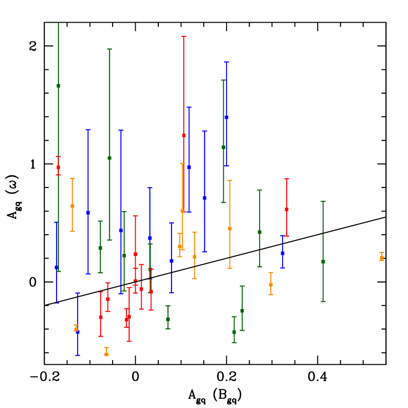
Figure 15.— Comparison of the two methods for calculating the angular covariance amplitude, A_gq  from Equation 7 and Equation 13, both with $\gamma=1.8$.

As has been noted in previous work, clustering statistics like B_gq  can be sensitive to the methodology used to calculate it, the choice of luminosity function and control fields. We therefore concentrate less on the absolute values of this parameter than on investigating any trends in the data, discussed in the following section.

5.2. Trends in Clustering Parameters

5.2.1 Correlation Amplitude

We investigate trends of galaxy-quasar clustering with quasar absolute $r$ magnitude, black hole mass, and [O III] line luminosity, as an indicator of AGN activity (Kauffmann et al., 2004). These properties are listed in Table 11. The values of M_r are derived from the $r$ listed in the SDSS DR9 catalog, with Galactic extinction calculated using the reddening values from Schlafly & Finkbeiner (2011) and the O’Donnell (1994) reddening law. We also applied a K-correction, calculated from the QSO composite spectrum of Vanden Berk et al. (2001) and the SDSS filter response curves. We collected black hole mass and [O III] $\lambda$5007 line luminosity measurements from the literature and list them in Table 11. Where the [O III] line luminosities do not exist in the literature, we downloaded the SDSS DR10 spectra for these objects and fit the H$\beta$ [O III]$\lambda$4959,5007 complex using the IRAF task specfit and list the resulting value in Table 11.

Table 11Sample Quasar Properties

QSO	Mr	log(MBH)	Refn.	[O III] Luminosity	Refn.
				erg/s $\times 10^{42}$
MRK586	-23.4	8.34	1	3.50	1
HS0624+690	-26.0	9.69	2	…	…
PG0844+349	-22.4	7.96	3	…	…
PG0923+201	-23.7	8.00	4	0.99	2
PG0953+414	-24.7	8.44	3	1.90	3
PG1116+215	-24.6	8.52	4	2.60	3
PG1307+085	-23.2	8.64	3	3.17	2
PG1404+226	-21.8	6.88	4	0.38	2
PG1444+407	-24.1	8.28	4	2.22	2
PG1545+210	-24.4	9.31	4	4.93	2
PG1612+261	-22.6	8.05	4	6.68	2
Q2141+175	-23.6	8.74	1	2.80	1

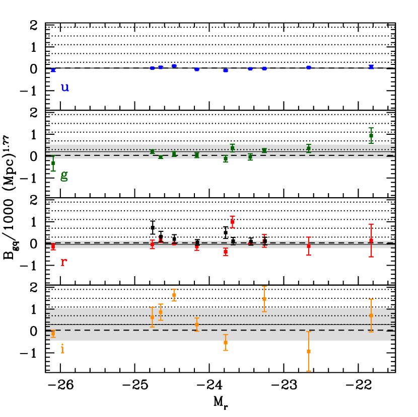
Figure 16.— B_gq in each filter versus quasar absolute r magnitude. Solid lines and shaded regions mark the mean and dispersion among all the values in a given filter, dotted lines show the expected correlation amplitude for Abell classes 0-4 (Yee & López-Cruz, 1999), and the dashed line marks the galaxy-galaxy correlation value from Davis & Peebles (1983). Black points show values from the literature listed in Table 7.

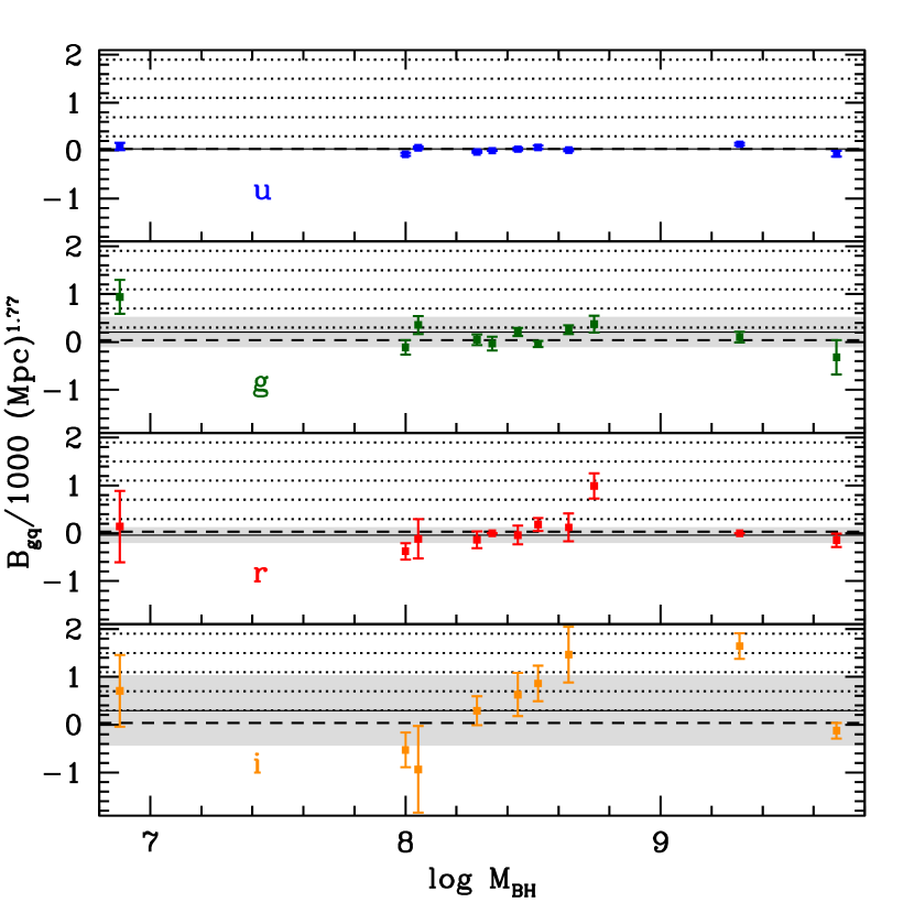
Figure 17.— As in Figure 16 but for B_gq in each filter versus quasar black hole mass

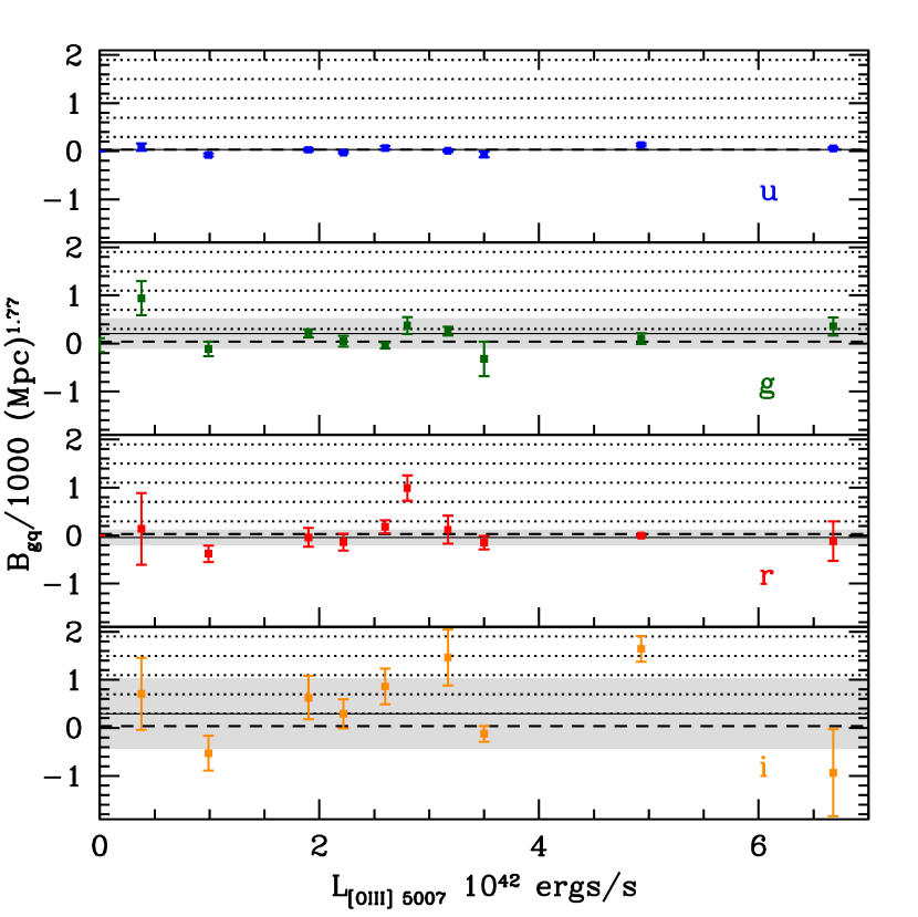
Figure 18.— As in Figure 16 but for B_gq in each filter versus quasar [O III] luminosity

Plots of these quasar properties with B_gq parameter are shown in Figures 16-18, but in no case do we find a significant trend of this clustering measure with any of the quasar properties.

5.2.2 Correlation Functions

We also investigate trends of the galaxy-quasar angular correlation function with quasar luminosity, black hole mass, and [O III] line luminosity by using the relative bias with respect to galaxies, $b_{gq}=(\omega_{gq}/\omega_{gg})^{1/2}$. Overall, we find $b_{gq}=(3.08\pm 0.51,1.49\pm 0.53,1.48\pm 0.29,0.95\pm 1.49)$ for $(u,g,r,i)$ for cross- and autocorrelation function solutions with fixed $\gamma=1.5$. The bias is only significantly greater than unity for the $u$ band and decreases with increasing wavelength, perhaps reflecting a trend seen for SDSS Sy 2 galaxies to lie in bluer environments than normal galaxies (Coldwell et al., 2014). This runs counter to a trend in the mean B_gq values quoted above, for which the $u$ band values are lowest and those in $i$ are the largest. This is driven by the large $i$ band B_gq values found for PG1545+201 and PG1307+085, the former being a radio loud quasar. That trend is less apparent for the radio quiet objects alone, and without PG1307+085 as well, the average $i$ band B_gq value drops to 129$\pm$238.

Table 12Galaxy-Galaxy and Galaxy-Quasar Correlations for each 90Prime Field

QSO	Filter	$\omega_{\rm gg}$	$\omega_{\rm gq}$
MRK586	$u$	0.151$\pm$0.036	0.08$\pm$1.08
	$g$	0.015$\pm$0.008	0.33$\pm$0.54
	$r$	0.072$\pm$0.006	0.07$\pm$0.47
HS0624+6907	$u$	0.071$\pm$0.024	-0.67$\pm$0.32
	$g$	0.387$\pm$0.055	0.67
	$r$	0.041$\pm$0.008	-0.50$\pm$0.24
	$i$	0.082$\pm$0.008	-0.98$\pm$0.01
PG0844+349	$u$	0.215$\pm$0.022	0.95$\pm$0.50
	$r$	0.006$\pm$0.003	-0.08$\pm$0.12
PG0923+201	$u$	0.150$\pm$0.019	0.19$\pm$0.53
	$g$	0.194$\pm$0.010	0.57$\pm$0.36
	$r$	0.223$\pm$0.011	0.95$\pm$0.32
	$i$	0.168$\pm$0.005	0.54$\pm$0.37
PG0953+414	$u$	0.206$\pm$0.012	0.32$\pm$0.47
	$g$	0.344$\pm$0.020	1.65$\pm$0.93
	$r$	0.246$\pm$0.008	-0.36$\pm$0.31
	$i$	0.270$\pm$0.004	0.19$\pm$0.30
PG1116+215	$u$	0.433$\pm$0.028	1.13$\pm$0.86
	$g$	0.630$\pm$0.039	1.80$\pm$1.40
	$r$	0.252$\pm$0.017	2.47$\pm$1.31
	$i$	0.127$\pm$0.006	0.83$\pm$0.61
PG1307+085	$u$	0.094$\pm$0.023	0.39$\pm$0.62
	$g$	0.158$\pm$0.015	0.42$\pm$0.53
	$r$	0.088$\pm$0.007	0.35$\pm$0.27
	$i$	0.104$\pm$0.005	0.01$\pm$0.19
PG1404+226	$u$	0.126$\pm$0.013	0.54$\pm$0.77
	$g$	0.123$\pm$0.007	0.24$\pm$0.87
	$r$	0.171$\pm$0.004	-0.15$\pm$0.28
	$i$	0.170$\pm$0.005	1.09$\pm$0.63
PG1444+407	$u$	0.257$\pm$0.022	0.36$\pm$0.96
	$g$	0.029$\pm$0.008	-0.03$\pm$0.30
	$r$	0.159$\pm$0.007	-0.35$\pm$0.20
	$i$	0.115$\pm$0.005	0.10$\pm$0.24
PG1545+210	$u$	-0.029$\pm$0.014	0.33$\pm$0.25
	$g$	0.257$\pm$0.018	-0.46$\pm$0.16
	$r$	0.063$\pm$0.006	-0.17$\pm$0.14
	$i$	0.093$\pm$0.005	0.09$\pm$0.21
PG1612+261	$u$	0.178$\pm$0.023	1.84$\pm$0.79
	$g$	0.432$\pm$0.009	-0.47$\pm$0.18
	$r$	0.203$\pm$0.006	-0.47$\pm$0.15
	$i$	0.199$\pm$0.005	-0.50$\pm$0.13
Q2141+175	$g$	0.172$\pm$0.009	-0.23$\pm$0.27
	$r$	0.389$\pm$0.008	0.17$\pm$0.39

The values of $\omega$ for each field and filter individually are listed in Table 12. For each field/filter where both the cross- and autocorrelation values are positive in the innermost bin, $\omega<1.167\arcmin$, we find no correlations in $b_{gq}$ with any of the quasar properties discussed above. Most fields for which both $\omega_{gq}$ and $\omega_{gg}$ within 1.167′ are positive show $b_{gq}>1$, but only a handful at $\gtrsim 2\sigma$: PG0844+349 and PG1612+261 in $u$, HS0624+690 in $g$, PG0923+201 and PG1116+215 in $r$, and PG1404+226 in $i$. For PG0844+349 and PG1612+261 the filters with $b_{gq}>1$ are the only filters with $\omega_{gq}>0$, for which $b_{gq}$ is defined. That the $u$ filters would show a large positive relative bias while all others show a quasar-galaxy anticorrelation may be indicative of bluer environments, although this does not hold for the HS0624+690 field, for which the $b_{gq}$ in $g$ is $1.31\pm 0.094$ but the values of $\omega_{gq}$ are negative in all other filters, including $u$. A few fields show $b_{gq}>1$ consistently in all filters (PG0923+201, PG1116+215) or in all filters but one: PG1307+085 ($i$), PG1404+226 ($r$). The bias seen in the $u$ band for the radio loud quasar PG1545+210 is negative, and not significantly greater than unity in any filter. Similarly, for the other radio loud AGN in our sample, Q2141+175, only $g$ and $r$ band data are available and neither shows a large bias. In $g$, $\omega_{gq}<0$, and in $r$ $b_{gq}=0.66\pm 0.75$.

6. Discussion

A somewhat contradictory picture emerges when we compare the results of the correlation function analysis to the calculated B_gq statistics. The fields that show the largest values of B_gq, PG1307+085, PG1545+210, PG0953+414 in the $i$ band, PG1404+226 in $g$, and Q2141+175 in $r$, all show relative biases that are consistent with unity. The PG0923+201 field showed an anticlustering B_gq signal in $u$ and $r$, but both filters give $b_{gq}>1$, with the $r$ band significant at $\sim 3\sigma$. We note that, in addition to a luminosity function dependence, the B_gq analysis probes a larger spatial scale than the relative bias calculation within 1.167′, corresponding to $\sim$10-40$h^{-1}$ kpc over the redshift range of the AGN in our sample.

Overall, as noted above in Section 5.1.1, the mean values of the correlation amplitude for 0.5 $h^{-1}$ Mpc scale clustering, while all consistent within the uncertainties with galaxy-galaxy clustering, show the largest signal in the $i$ band, B_gq=295$\pm$260. The correlation function analysis, on the other hand, probing $\sim$10-40$h^{-1}$ kpc scales shows the largest bias for quasar galaxy clustering in the $u$ band, with galaxy clustering around quasars a factor of 3 larger than the galaxy autocorrelation signal at these scales. This suggests that different galaxy types may cluster around quasars on different scales. Some earlier studies have seen clustering signals at small scales and differences in galaxy populations near quasars. In a future paper, we will use the multi-band data to calculate photometric redshifts for the galaxies in our sample, and investigate trends in the clustering parameters with galaxy types determined with these redshifts.

The basic trends in our results are consistent with earlier findings that quasars cluster like L^∗ galaxies, and indeed like galaxies up to 2 magnitudes fainter than L^∗. We also confirm that there are no significant trends with quasar luminosity (Finn et al., 2001; Serber et al., 2006; Coil et al., 2007), though unlike Serber et al. (2006), we also find that the lack of luminosity dependence holds at small as well as large spatial scales. In our sample of broad line AGN, we do not find the trend for AGN with lower [O III] luminosities to have larger clustering signals as seen in SDSS narrow line AGN (Wake et al., 2004).

Thus, the mechanism driving accretion onto the central black holes in these objects is not imprinted on their large scale galaxy environments. This may be due to a non-merger mode in fueling the central black holes or to a delay in the onset of nuclear activity from the time of the initial galaxy interactions which triggered its fueling.

Appendix A Notes on Individual Objects

In this section, we outline notes on each of our 90Prime fields, based on previous studies of the quasar fields and host galaxies, searches for nearby objects in the NASA Extragalactic Database (NED), and the results of our calculations of the correlation amplitude, B_gq. We refer the reader to Table 7 and Figures 11–18.

A.1. Mrk 586, $z=0.155$

The field of this radio quiet object has been imaged previously in narrow band [O iii] by Stockton & MacKenty (1987) and in the optical (B,$g$,$i$ filters) by Kirhakos et al. (1994) using the Palomar 1.5 m (image sizes $\sim$3′ $\times$ 3′) who note four galaxies in this field, including a large disk galaxy (NAB 0205+02: 06) at a projected separation of 15.6 $h^{-1}$ kpc.

The quasar host was studied by (Bahcall et al., 1997) using the HST/ Wide Field/Planetary Camera-2 (WFPC2) and the F606W filter. The host is disk-like and the AGN has a companion with jet-like structure at a projected distance of 23 $h^{-1}$ kpc (Stockton & MacKenty, 1987; Bahcall et al., 1997). There is no evidence of tidal features to suggest a direct interaction.

A NED search reveals $\sim$17 galaxy clusters, groups, or candidates, within 50′ of the quasar. The cluster with the smallest angular separation from the quasar (7.7′) is NSCS J020723+024645, which lies at $z=0.37$.

The B_gq we calculate from the 90Prime $r$ band image is identically zero because the number of galaxies detected at 5$\sigma$ within 0.5 $h^{-1}$ Mpc of the quasar exactly equals the median number found in 871 control fields. This is consistent with the values found by both McLure & Dunlop (2001b) and Finn et al. (2001) from the HST/WFPC2 images in the F606W filter, 93$\pm$161 and 13$\pm$82, respectively, and with the values calculated from the 90Prime $u$ and $g$ band images, -3$\pm$6 and -36$\pm$137, respectively. We have no 90Prime data of this field in the $i$ band.

A.2. HS0624+690, $z=0.370$, QSO

The host of this radio quiet quasar is an elliptical galaxy (Floyd et al., 2004). Kirhakos et al. (1994) identify six galaxies in their ground-based optical images within the $\sim$3′ $\times$ 3′ frame. From NED, we find that within 50′ of the quasar, there is one known galaxy cluster, Abell 0557 (redshift unknown), at 8.03′ separation from the quasar.

All the B_gq values we calculate for this field are less than zero, indicating an underdensity of galaxies within 0.5 $h^{-1}$ Mpc of the quasar, however, none of these underdensities is significantly less than B_gg at $>2\sigma$. We conclude that the field around this object is consistent with the field. A caveat to this is that HS0624+690 is the the highest redshift AGN in our sample, and the limiting magnitudes of the $u$ and $g$ coadded images are not significantly fainter than M^∗ at the quasar redshift, M^∗ + 0.7 and M^∗ + 0.1, respectively, so we are not reaching as far down the luminosity function for this field as the others in the sample.

A.3. PG0844+349, $z=0.064$

This radio quiet object has a host with bulge+disk structure, showing no bar, but some evidence of morphological disturbance from deep H-band imaging (Guyon et al., 2006; Veilleux et al., 2009). This object qualifies as having a bright interacting companion (H band luminosity greater than 1/10 L_∗ and projected distance within 24 $h^{-1}$ kpc McLeod & Rieke (1994b), though it is not likely currently undergoing a strong interaction since Veilleux et al. (2009) classify this object as a post-merger object with a single nucleus. Also, from the [O ii] measurement of Wilkes et al. (1999), Ho (2005) estimates a star formation rate of the host galaxy of less than 1.6 M_⊙ yr^-1. Within a 50′ radius around this quasar, NED returns 58 galaxy clusters, groups, or candidates.

A.4. PG0923+201, $z=0.192$

The host of this radio quiet AGN is an elliptical galaxy with no evidence of a bar or of morphological disturbance from an interaction with a companion (Dunlop et al., 2003; Guyon et al., 2006; Veilleux et al., 2009). Previous authors have note the presence of two bright galaxies within 16 $h^{-1}$ kpc of the quasar and have suggested it is a member of a small group (Heckman et al., 1984; McLeod & Rieke, 1994b; Bahcall et al., 1997). Indeed, the compact group SDSSCGB 30540 ($z=0.19$) identified by McConnachie et al. (2009) in the SDSS DR6 has a redshift consistent with that of PG0923+201. While the quasar is not listed as a group member in their catalog, it has a separation of $\sim$23 $h^{-1}$ kpc from the group center. There are $\sim$45 other galaxy clusters or groups within 50′ of this quasar.

Our B_gq values from the $r$ and $i$ band frames, -377$\pm$130 and -529$\pm$291, are inconsistent with those of McLure & Dunlop (2001b) and Finn et al. (2001) at the 3.5-4$\sigma$ level. These authors find moderately significant overdensities in this field while we see underdensities in all filters, of increasing magnitude from $u$ to $i$. This underdensity is surprising if the quasar is in fact associated with SDSSCGB 30540.

A.5. PG0953+414, $z=0.234$

Dunlop et al. (2003) classify the host galaxy of this radio quiet AGN as an elliptical, while others (Bahcall et al., 1997; Guyon et al., 2006) have found it to show disk-like structure but to be too faint to classify reliably. Kirhakos et al. (1994) find 22 likely galaxies in their optical images described above in Sec. A.1.

There are 54 galaxy groups, clusters or candidates within 50′ of this quasar, one of which, GMBCG J149.20633+41.27869, has a projected separation of only 1.455′, though it lies well behind PG0953+414, at $z=0.362$. A second cluster, WHL J095714.9+411700, is separated by 4.532′ from the quasar and has a redshift $z=0.446$.

Our $i$ band result for B_gq is consistent with the result of McLure & Dunlop (2001b) using HST/WFPC2 F675W. Both values are large, $\sim 600-700$, but with large statistical uncertainty, $\sim 300-400$. The $g$ band value for this field, 207$\pm$101, is one of $\sim 1/4$ of the B_gq results that are significantly greater than B_gg, while the B_gq result from the 90Prime $r$ band image is negative but consistent with B_gg, and consistent with the value found by Finn et al. (2001) from HST/WFPC2 F606W data within the uncertainties.

A.6. PG1116+215, $z=0.177$

PSF problems affected the deep H band imaging of the host galaxy of this radio quiet object, with some conflicting results. Guyon et al. (2006) find that the host is disk-like and asymmetric with some evidence for a disturbance, while Veilleux et al. (2009) find that it shows no sprial arms or bar or morphological disturbance and classify it as an old merger, in agreement with the optical imaging (Bahcall et al., 1997).

There are $\sim$68 galaxy clusters, groups, or candidates within this field around PG1116+215. The two with the smallest separations from the quasar (0.28′ and 1.92′) are ZwCl 1116.5+2136 and SDSSCGB 16808 (McConnachie et al., 2009), both with unknown redshifts. However, one cluster found in the SDSS data, MaxBCG J169.85817+21.20845, lies at 7.9′ separation and has a redshift marginally consistent with PG1116+215, $z_{\rm phot}=0.170$. The relatively large projected and redshift separations, $\sim$1 $h^{-1}$ Mpc, and $\sim$1630 km s^-1, place it toward the periphery of this cluster if it is associated with it at all.

Our results for B_gq from the 90Prime $r$ band image, 186$\pm$134, is consistent with McLure & Dunlop (2001b) and Finn et al. (2001) within the large statistical uncertainties. The B_gq values found in the $u$ and $g$ filters are also consistent with B_gg, strengthening the conclusion that PG1116+215 lies in the outer regions or even outside the cluster potential of MaxBCG J169.85817+21.20845. However, the result for the $i$ band, 863$\pm$461, presents a contradiction to this picture as it is greater than B_gg, more consistent with an Abell class 1 environment (McLure & Dunlop, 2001b).

A.7. PG1307+085, $z=0.155$

The host galaxy of this radio quiet quasar is an elliptical with no evidence of a disturbance (Bahcall et al., 1997; Hamilton et al., 2002; Guyon et al., 2006; Veilleux et al., 2009). The center of the $z=0.14$ cluster GMBCG J197.43444+08.33445 (Koester et al., 2007) lies at a projected separation of only 43.5″ from the quasar. Given the redshift separation it is unlikely that PG1307+085 is a cluster member but many galaxies in the 90Prime field likely are.

Our results for B_gq in the $r$ band are consistent with McLure & Dunlop (2001b) and Finn et al. (2001) within the large uncertainties. The $i$ band result for B_gq for this field is very large, 1461$\pm$778. The B_gq value found for the $g$ band, 259$\pm$120, is also large relative to other filters. The presence of GMBCG J197.43444+08.33445 in the foreground may be influencing the galaxy counts for this field, though it is not clear why this should only be the case for the $g$ and $i$ filters and not $u$ and $r$, which both show B_gq consistent with B_gg.

A.8. PG1404+226, $z=0.098$, NLS1

Ho (2005) conclude that the host galaxy of this quasar has a very low star formation rate, $<$0.14 M_⊙ yr^-1, based on the [O ii] measurement of Kuraszkiewicz et al. (2000). It also has a low black hole mass, $\log(\rm M_{\rm BH}/\rm M_{\odot})=6.88$, as estimated from the H$\beta$ line width (Vestergaard & Peterson, 2006). McLeod & Rieke (1994a) find that an exponential profile with a scale length of 2.98 $h^{-1}$ kpc gives a reasonable fit to their H band image of this AGN.

There are $\sim$50 clusters, groups, or candidates identified in the 50′ around PG1404+226, including five compact groups of McConnachie et al. (2009) with separations less than $\sim$22′ and unknown redshift. The cluster WHL J140609.9+221605 has a separation of 8.17′ from the quasar and a redshift of $z=0.393$.

All values of B_gq for this field are consistent with B_gg, except in the $g$ band, where we find B_gq=942$\pm$522.

A.9. PG1444+407, $z=0.267$

The morphology of the host galaxy of this radio quiet AGN is somewhat ambiguous. Bahcall et al. (1997) confirm the possible presence of a bar suggested by Hutchings & Neff (1992) as the result of an old merger stage. Interestingly, based on the [O ii] measurement of Baldwin et al. (1989), Ho (2005) infer a fairly high star formation rate in the host of 19.4 M_⊙ yr^-1, on the order of that found for interacting and luminous IR galaxies.

There are 48 galaxy clusters, groups, or candidates within 50′ of the quasar, with the closest, ZwCl 1443.8+4043, lying at a separation of 12.6′, but unknown redshift.

For this field we find B_gq values in the $g$, $r$, and $i$ filters consistent with B_gg. The $r$ band result is consistent with small positive values with large statistical uncertainties from the other studies of McLure & Dunlop (2001b) and Finn et al. (2001). In the $u$ band, we find a B_gq $<$ B_gg by more than $2\sigma$, reflecting the general trend for the $u$ band to show the smallest values of B_gq, though we note that the limiting $u$ magnitude for this field corresponds to M^∗+1.4 at the redshift of this AGN rather than to M^∗+2.

A.10. PG1545+210 (3C 323.1), $z=0.264$

This FRII radio loud AGN has an elliptical host galaxy (McLeod & Rieke, 1994b; Bahcall et al., 1997) with a faint elliptical companion galaxy at a projected separation of 7.7 $h^{-1}$ kpc. Ho (2005) finds a moderately large star formation rate of 9.7 M_⊙ yr^-1 in the host galaxy, based on the [O ii] measurement of Wills et al. (1993). From population synthesis model fits to the optical spectrum of the companion, Canalizo & Stockton (1997) report evidence of a possible interaction 2.3 Gyr ago. This quasar was found to have a rich cluster environment (Abell class 1) by Oemler et al. (1972), and Kirhakos et al. (1994) find 22 likely galaxies in their optical images described above in Sec. A.1. It is located 1.96′ away from another broad line AGN at a very similar redshift (SDSS J154749.70+205056.5, $z=0.26547$).

These AGNs are likely members of the X-ray indentified cluster ZwCl 1545.1+2104 ($z=0.266$, Piffaretti et al. (2011)), also found in the SDSS DR7 data ($z=0.26735$, Hao et al. (2010)). There are $\sim$70 other galaxy clusters, groups, or candidates within 50′ of PG1545+210. We note that this field also contains the highest number of $z<0.5$ AGN of any of the other 90Prime fields, listed in Table 9.

Here we a B_gq value in $g$ consistent with B_gg, and the $r$ band value identically zero, as for MRK 586. This is in agreement with the HST/WFPC2 F606W results of McLure & Dunlop (2001b). However, given the smaller uncertainty quoted by Finn et al. (2001), our value $r$ band value differs from their positive results by $\sim 3\sigma$. As for PG1307+085, we find a very large value of B_gq for this field in the $i$ band and a much smaller but significant signal in $u$, consistent with its known cluster environment. The limiting $u$ magnitude for this field corresponds to M^∗+1.7 at the redshift of this AGN, rather than reaching to M^∗+2.

A.11. PG1612+261, $z=0.131$

McLeod & Rieke (1994a) find that an exponential profile with a scale length of 1.16 $h^{-1}$ kpc gives a reasonable fit to their H band image of this AGN and its immediate environment meets the criteria of McLeod & Rieke (1994b) for bright interacting companion. (See Sec. A.3.)

It may be associated with the cluster NSC J161419+260832 ($z=0.1396$) but given the velocity separation and the $\sim$0.5 $h^{-1}$ Mpc separation on the sky from the reported cluster center, it is likely on the periphery. There are $\sim$47 other unique galaxy clusters, groups or candidates within 50′ of the quasar found in NED.

The $g$ band B_gq value for this field, 354$\pm$237, is marginally greater than B_gg, but it is consistent with B_gg in $u$, $r$ and $i$. The most closely separated $z<1$ QSO in this field, SDSS J161335.33+263127.7, lies at $z=0.708$ and $\sim$28.5′.

A.12. [HB89] 2141+175, $z=0.211$

This radio loud AGN has an elliptical host, with some suggestion of an interacting companion (Hutchings & Neff, 1992; Dunlop et al., 2003). There is only one known galaxy cluster in this field, within 46′ of this quasar.

We have no $i$ band image from 90Prime to compare with the HST/WFPC2 F675W result of McLure & Dunlop (2001b), but our large $r$ band result, 991$\pm$355 is larger than theirs by $>$2.5$\sigma$.

References

- Adelberger & Steidel (2005) Adelberger, K. L., & Steidel, C. C. 2005, ApJ, 627, L1
- Alonso et al. (2007) Alonso, M. S., Lambas, D. G., Tissera, P., & Coldwell, G. 2007, MNRAS, 375, 1017
- Bahcall et al. (1997) Bahcall, J. N., Kirhakos, S., Saxe, D. H., & Schneider, D. P. 1997, ApJ, 479, 642
- Baldwin et al. (1989) Baldwin, J. A., Wampler, E. J., & Gaskell, C. M. 1989, ApJ, 338, 630
- Barnes & Hernquist (1992) Barnes, J. E., & Hernquist, L. 1992, ARA&A, 30, 705
- Barr et al. (2003) Barr, J. M., Bremer, M. N., Baker, J. C., & Lehnert, M. D. 2003, MNRAS, 346, 229
- Bennert et al. (2008) Bennert, N., Canalizo, G., Jungwiert, B., et al. 2008, ApJ, 677, 846
- Bertin & Arnouts (1996) Bertin, E., & Arnouts, S. 1996, A&AS, 117, 393
- Bertin et al. (2002) Bertin, E., Mellier, Y., Radovich, M., et al. 2002, in Astronomical Society of the Pacific Conference Series, Vol. 281, Astronomical Data Analysis Software and Systems XI, ed. D. A. Bohlender, D. Durand, & T. H. Handley, 228
- Best et al. (2005) Best, P. N., Kauffmann, G., Heckman, T. M., et al. 2005, MNRAS, 362, 25
- Blanton & Roweis (2007) Blanton, M. R., & Roweis, S. 2007, AJ, 133, 734
- Brown et al. (2001) Brown, M. J. I., Boyle, B. J., & Webster, R. L. 2001, AJ, 122, 26
- Canalizo et al. (2007) Canalizo, G., Bennert, N., Jungwiert, B., et al. 2007, ApJ, 669, 801
- Canalizo & Stockton (1997) Canalizo, G., & Stockton, A. 1997, ApJ, 480, L5
- Coil et al. (2007) Coil, A. L., Hennawi, J. F., Newman, J. A., Cooper, M. C., & Davis, M. 2007, ApJ, 654, 115
- Coil et al. (2004) Coil, A. L., Newman, J. A., Kaiser, N., et al. 2004, ApJ, 617, 765
- Coil et al. (2009) Coil, A. L., Georgakakis, A., Newman, J. A., et al. 2009, ApJ, 701, 1484
- Coldwell et al. (2014) Coldwell, G. V., Gurovich, S., Díaz Tello, J., Söchting, I. K., & Lambas, D. G. 2014, MNRAS, 437, 1199
- Coldwell & Lambas (2003) Coldwell, G. V., & Lambas, D. G. 2003, MNRAS, 344, 156
- Coldwell & Lambas (2006) —. 2006, MNRAS, 371, 786
- Coldwell et al. (2002) Coldwell, G. V., Martínez, H. J., & Lambas, D. G. 2002, MNRAS, 336, 207
- Constantin et al. (2008) Constantin, A., Hoyle, F., & Vogeley, M. S. 2008, ApJ, 673, 715
- Constantin & Vogeley (2006) Constantin, A., & Vogeley, M. S. 2006, ApJ, 650, 727
- Cool et al. (2012) Cool, R. J., Eisenstein, D. J., Kochanek, C. S., et al. 2012, ApJ, 748, 10
- Croom & Shanks (1999) Croom, S. M., & Shanks, T. 1999, MNRAS, 303, 411
- Croom et al. (2005) Croom, S. M., Boyle, B. J., Shanks, T., et al. 2005, MNRAS, 356, 415
- Croton et al. (2006) Croton, D. J., Springel, V., White, S. D. M., et al. 2006, MNRAS, 365, 11
- Davis & Peebles (1983) Davis, M., & Peebles, P. J. E. 1983, ApJ, 267, 465
- Di Matteo et al. (2005) Di Matteo, T., Springel, V., & Hernquist, L. 2005, Nature, 433, 604
- Dressler (1980) Dressler, A. 1980, ApJ, 236, 351
- Dunlop et al. (2003) Dunlop, J. S., McLure, R. J., Kukula, M. J., et al. 2003, MNRAS, 340, 1095
- Ellingson et al. (1991) Ellingson, E., Yee, H. K. C., & Green, R. F. 1991, ApJ, 371, 49
- Ellison et al. (2013) Ellison, S. L., Mendel, J. T., Patton, D. R., & Scudder, J. M. 2013, MNRAS, 435, 3627
- Faber et al. (2007) Faber, S. M., Willmer, C. N. A., Wolf, C., et al. 2007, ApJ, 665, 265
- Ferrarese & Merritt (2000) Ferrarese, L., & Merritt, D. 2000, ApJ, 539, L9
- Finn et al. (2001) Finn, R. A., Impey, C. D., & Hooper, E. J. 2001, ApJ, 557, 578
- Fisher et al. (1996) Fisher, K. B., Bahcall, J. N., Kirhakos, S., & Schneider, D. P. 1996, ApJ, 468, 469
- Floyd et al. (2004) Floyd, D. J. E., Kukula, M. J., Dunlop, J. S., et al. 2004, MNRAS, 355, 196
- Gabor et al. (2009) Gabor, J. M., Impey, C. D., Jahnke, K., et al. 2009, ApJ, 691, 705
- Gebhardt et al. (2000) Gebhardt, K., Bender, R., Bower, G., et al. 2000, ApJ, 539, L13
- Gilli et al. (2003) Gilli, R., Cimatti, A., Daddi, E., et al. 2003, ApJ, 592, 721
- Gilli et al. (2009) Gilli, R., Zamorani, G., Miyaji, T., et al. 2009, A&A, 494, 33
- Granato et al. (2004) Granato, G. L., De Zotti, G., Silva, L., Bressan, A., & Danese, L. 2004, ApJ, 600, 580
- Grogin et al. (2005) Grogin, N. A., Conselice, C. J., Chatzichristou, E., et al. 2005, ApJ, 627, L97
- Groth & Peebles (1977) Groth, E. J., & Peebles, P. J. E. 1977, ApJ, 217, 385
- Gunn & Stryker (1983) Gunn, J. E., & Stryker, L. L. 1983, ApJS, 52, 121
- Guyon et al. (2006) Guyon, O., Sanders, D. B., & Stockton, A. 2006, ApJS, 166, 89
- Haiman et al. (2004) Haiman, Z., Ciotti, L., & Ostriker, J. P. 2004, ApJ, 606, 763
- Hall et al. (1998) Hall, P. B., Green, R. F., & Cohen, M. 1998, ApJS, 119, 1
- Hamilton et al. (2002) Hamilton, T. S., Casertano, S., & Turnshek, D. A. 2002, ApJ, 576, 61
- Hao et al. (2010) Hao, J., McKay, T. A., Koester, B. P., et al. 2010, ApJS, 191, 254
- Heckman et al. (1984) Heckman, T. M., Bothun, G. D., Balick, B., & Smith, E. P. 1984, AJ, 89, 958
- Hennawi et al. (2006) Hennawi, J. F., Strauss, M. A., Oguri, M., et al. 2006, AJ, 131, 1
- Hickox et al. (2009) Hickox, R. C., Jones, C., Forman, W. R., et al. 2009, ApJ, 696, 891
- Ho (2005) Ho, L. C. 2005, ApJ, 629, 680
- Ho & Kim (2009) Ho, L. C., & Kim, M. 2009, ApJS, 184, 398
- Hopkins & Hernquist (2006) Hopkins, P. F., & Hernquist, L. 2006, ApJS, 166, 1
- Hopkins et al. (2006a) Hopkins, P. F., Hernquist, L., Cox, T. J., et al. 2006a, ApJS, 163, 1
- Hopkins et al. (2008) Hopkins, P. F., Hernquist, L., Cox, T. J., & Kereš, D. 2008, ApJS, 175, 356
- Hopkins et al. (2006b) Hopkins, P. F., Somerville, R. S., Hernquist, L., et al. 2006b, ApJ, 652, 864
- Hutchings & Neff (1992) Hutchings, J. B., & Neff, S. G. 1992, AJ, 104, 1
- Infante (1994) Infante, L. 1994, A&A, 282, 353
- Kauffmann & Haehnelt (2000) Kauffmann, G., & Haehnelt, M. 2000, MNRAS, 311, 576
- Kauffmann et al. (2004) Kauffmann, G., White, S. D. M., Heckman, T. M., et al. 2004, MNRAS, 353, 713
- Kauffmann et al. (2003) Kauffmann, G., Heckman, T. M., Tremonti, C., et al. 2003, MNRAS, 346, 1055
- Kewley et al. (2006) Kewley, L. J., Groves, B., Kauffmann, G., & Heckman, T. 2006, MNRAS, 372, 961
- Kinney et al. (1996) Kinney, A. L., Calzetti, D., Bohlin, R. C., et al. 1996, ApJ, 467, 38
- Kirhakos et al. (1994) Kirhakos, S., Sargent, W. L. W., Schneider, D. P., et al. 1994, PASP, 106, 646
- Koester et al. (2007) Koester, B. P., McKay, T. A., Annis, J., et al. 2007, ApJ, 660, 239
- Kuraszkiewicz et al. (2000) Kuraszkiewicz, J., Wilkes, B. J., Brandt, W. N., & Vestergaard, M. 2000, ApJ, 542, 631
- Labita et al. (2006) Labita, M., Treves, A., Falomo, R., & Uslenghi, M. 2006, MNRAS, 373, 551
- Landy & Szalay (1993) Landy, S. D., & Szalay, A. S. 1993, ApJ, 412, 64
- Li et al. (2008) Li, C., Kauffmann, G., Heckman, T. M., White, S. D. M., & Jing, Y. P. 2008, MNRAS, 385, 1915
- Li et al. (2006) Li, C., Kauffmann, G., Wang, L., et al. 2006, MNRAS, 373, 457
- Limber (1953) Limber, D. N. 1953, ApJ, 117, 134
- Longair & Seldner (1979) Longair, M. S., & Seldner, M. 1979, MNRAS, 189, 433
- Loveday et al. (2012) Loveday, J., Norberg, P., Baldry, I. K., et al. 2012, MNRAS, 420, 1239
- Lupton et al. (1999) Lupton, R. H., Gunn, J. E., & Szalay, A. S. 1999, AJ, 118, 1406
- Marconi & Hunt (2003) Marconi, A., & Hunt, L. K. 2003, ApJ, 589, L21
- McConnachie et al. (2009) McConnachie, A. W., Patton, D. R., Ellison, S. L., & Simard, L. 2009, MNRAS, 395, 255
- McLeod & Rieke (1994a) McLeod, K. K., & Rieke, G. H. 1994a, ApJ, 420, 58
- McLeod & Rieke (1994b) —. 1994b, ApJ, 431, 137
- McLeod & Rieke (1995) —. 1995, ApJ, 454, L77
- McLeod et al. (1999) McLeod, K. K., Rieke, G. H., & Storrie-Lombardi, L. J. 1999, ApJ, 511, L67
- McLure & Dunlop (2001a) McLure, R. J., & Dunlop, J. S. 2001a, MNRAS, 327, 199
- McLure & Dunlop (2001b) —. 2001b, MNRAS, 321, 515
- McLure & Dunlop (2002) —. 2002, MNRAS, 331, 795
- McLure et al. (1999) McLure, R. J., Kukula, M. J., Dunlop, J. S., et al. 1999, MNRAS, 308, 377
- Montero-Dorta et al. (2009) Montero-Dorta, A. D., Croton, D. J., Yan, R., et al. 2009, MNRAS, 392, 125
- Myers et al. (2007a) Myers, A. D., Brunner, R. J., Nichol, R. C., et al. 2007a, ApJ, 658, 85
- Myers et al. (2007b) Myers, A. D., Brunner, R. J., Richards, G. T., et al. 2007b, ApJ, 658, 99
- Myers et al. (2006) —. 2006, ApJ, 638, 622
- O’Donnell (1994) O’Donnell, J. E. 1994, ApJ, 422, 158
- Oemler et al. (1972) Oemler, Jr., A., Gunn, J. E., & Oke, J. B. 1972, ApJ, 176, L47
- Peterson et al. (2004) Peterson, B. M., Ferrarese, L., Gilbert, K. M., et al. 2004, ApJ, 613, 682
- Piffaretti et al. (2011) Piffaretti, R., Arnaud, M., Pratt, G. W., Pointecouteau, E., & Melin, J.-B. 2011, A&A, 534, A109
- Porciani et al. (2004) Porciani, C., Magliocchetti, M., & Norberg, P. 2004, MNRAS, 355, 1010
- Porciani & Norberg (2006) Porciani, C., & Norberg, P. 2006, MNRAS, 371, 1824
- Prescott et al. (2009) Prescott, M., Baldry, I. K., & James, P. A. 2009, MNRAS, 397, 90
- Ramos Almeida et al. (2013) Ramos Almeida, C., Bessiere, P. S., Tadhunter, C., et al. 2013, ArXiv e-prints, arXiv:1308.4725
- Ross et al. (2009) Ross, N. P., Shen, Y., Strauss, M. A., et al. 2009, ApJ, 697, 1634
- Sabater et al. (2013) Sabater, J., Best, P. N., & Argudo-Fernández, M. 2013, MNRAS, 430, 638
- Sabater et al. (2012) Sabater, J., Verdes-Montenegro, L., Leon, S., Best, P., & Sulentic, J. 2012, A&A, 545, A15
- Sanders et al. (1988) Sanders, D. B., Soifer, B. T., Elias, J. H., et al. 1988, ApJ, 325, 74
- Schlafly & Finkbeiner (2011) Schlafly, E. F., & Finkbeiner, D. P. 2011, ApJ, 737, 103
- Serber et al. (2006) Serber, W., Bahcall, N., Ménard, B., & Richards, G. 2006, ApJ, 643, 68
- Shang et al. (2007) Shang, Z., Wills, B. J., Wills, D., & Brotherton, M. S. 2007, AJ, 134, 294
- Shen et al. (2007) Shen, Y., Strauss, M. A., Oguri, M., et al. 2007, AJ, 133, 2222
- Shen et al. (2009) Shen, Y., Strauss, M. A., Ross, N. P., et al. 2009, ApJ, 697, 1656
- Shen et al. (2010) Shen, Y., Hennawi, J. F., Shankar, F., et al. 2010, ApJ, 719, 1693
- Silverman et al. (2008) Silverman, J. D., Mainieri, V., Lehmer, B. D., et al. 2008, ApJ, 675, 1025
- Silverman et al. (2009) Silverman, J. D., Kovač, K., Knobel, C., et al. 2009, ApJ, 695, 171
- Smith et al. (1995) Smith, R. J., Boyle, B. J., & Maddox, S. J. 1995, MNRAS, 277, 270
- Söchting et al. (2002) Söchting, I. K., Clowes, R. G., & Campusano, L. E. 2002, MNRAS, 331, 569
- Söchting et al. (2004) —. 2004, MNRAS, 347, 1241
- Somerville et al. (2008) Somerville, R. S., Hopkins, P. F., Cox, T. J., Robertson, B. E., & Hernquist, L. 2008, MNRAS, 391, 481
- Springel et al. (2005a) Springel, V., Di Matteo, T., & Hernquist, L. 2005a, ApJ, 620, L79
- Springel et al. (2005b) —. 2005b, MNRAS, 361, 776
- Stockton & MacKenty (1987) Stockton, A., & MacKenty, J. W. 1987, ApJ, 316, 584
- Teng & Veilleux (2010) Teng, S. H., & Veilleux, S. 2010, ApJ, 725, 1848
- Teplitz et al. (1999) Teplitz, H. I., McLean, I. S., & Malkan, M. A. 1999, ApJ, 520, 469
- Tremaine et al. (2002) Tremaine, S., Gebhardt, K., Bender, R., et al. 2002, ApJ, 574, 740
- Vanden Berk et al. (2001) Vanden Berk, D. E., Richards, G. T., Bauer, A., et al. 2001, AJ, 122, 549
- Veilleux et al. (2009) Veilleux, S., Rupke, D. S. N., Kim, D.-C., et al. 2009, ApJS, 182, 628
- Véron-Cetty & Véron (2010) Véron-Cetty, M.-P., & Véron, P. 2010, A&A, 518, A10
- Vestergaard & Peterson (2006) Vestergaard, M., & Peterson, B. M. 2006, ApJ, 641, 689
- Volonteri et al. (2003) Volonteri, M., Haardt, F., & Madau, P. 2003, ApJ, 582, 559
- Wake et al. (2004) Wake, D. A., Miller, C. J., Di Matteo, T., et al. 2004, ApJ, 610, L85
- Wilkes et al. (1999) Wilkes, B. J., Kuraszkiewicz, J., Green, P. J., Mathur, S., & McDowell, J. C. 1999, ApJ, 513, 76
- Williams et al. (2004) Williams, G. G., Olszewski, E., Lesser, M. P., & Burge, J. H. 2004, in Society of Photo-Optical Instrumentation Engineers (SPIE) Conference Series, Vol. 5492, Ground-based Instrumentation for Astronomy, ed. A. F. M. Moorwood & M. Iye, 787–798
- Wills et al. (1993) Wills, B. J., Netzer, H., Brotherton, M. S., et al. 1993, ApJ, 410, 534
- Wold et al. (2003) Wold, M., Armus, L., Neugebauer, G., Jarrett, T. H., & Lehnert, M. D. 2003, AJ, 126, 1776
- Wold et al. (2001) Wold, M., Lacy, M., Lilje, P. B., & Serjeant, S. 2001, MNRAS, 323, 231
- Wyithe & Loeb (2003) Wyithe, J. S. B., & Loeb, A. 2003, ApJ, 595, 614
- Yates et al. (1989) Yates, M. G., Miller, L., & Peacock, J. A. 1989, MNRAS, 240, 129
- Yee & Ellingson (1993) Yee, H. K. C., & Ellingson, E. 1993, ApJ, 411, 43
- Yee & Green (1984) Yee, H. K. C., & Green, R. F. 1984, ApJ, 280, 79
- Yee & López-Cruz (1999) Yee, H. K. C., & López-Cruz, O. 1999, AJ, 117, 1985