Convex Combination
of Ordinary Least Squares and Two-stage Least Squares Estimators

Abstract

In the presence of confounders, the ordinary least squares (OLS) estimator is known to be biased. This problem can be remedied by using the two-stage least squares (TSLS) estimator, based on the availability of valid instrumental variables (IVs). This reduction in bias, however, is offset by an increase in variance. Under standard assumptions, the OLS has indeed a larger bias than the TSLS estimator; and moreover, one can prove that the sample variance of the OLS estimator is no greater than the one of the TSLS. Therefore, it is natural to ask whether one could combine the desirable properties of the OLS and TSLS estimators. Such a trade-off can be achieved through a convex combination of these two estimators, thereby producing our proposed convex least squares (CLS) estimator. The relative contribution of the OLS and TSLS estimators is here chosen to minimize a sample estimate of the mean squared error (MSE) of their convex combination. This proportion parameter is proved to be unique, whenever the OLS and TSLS differ in MSEs. Remarkably, we show that this proportion parameter can be estimated from the data, and that the resulting CLS estimator is consistent. We also show how the CLS framework can incorporate other asymptotically unbiased estimators, such as the jackknife IV estimator (JIVE). The finite-sample properties of the CLS estimator are investigated using Monte Carlo simulations, in which we independently vary the amount of confounding and the strength of the instrument. Overall, the CLS estimator is found to outperform the TSLS estimator in terms of MSE. The method is also applied to a classic data set from econometrics, which models the financial return to education.

18 blue t1This work was supported by an MRC project grant MR/K006185/1, Landau et al. (2013-2016) entitled “Developing methods for understanding mechanism in complex interventions.” We also would like to thank Stephen Burgess, Paul Clarke, Graham Dunn, Andrew Pickles, and Ian White for useful suggestions and discussions. 0000.0000

1 Introduction

Instrumental variables (IVs) estimation is one of the cornerstones of modern econometric theory. The use of IVs has been described as “only second to ordinary least squares (OLS) in terms of methods used in empirical economic research” (Wooldridge, 2002, p.89). This ranking of estimation techniques naturally leads to the following methodological questions: When should we prefer IV estimation over OLS? Is it always preferable to use an instrument even though this may substantially increase the variance of the resulting estimator?

In fields including econometrics and the social sciences, and in some medical disciplines such as psychiatry, the direct randomized allocation of subjects to different experimental conditions is rarely possible, thereby preventing such scientists from inferring causal relations. Without adequate experimental manipulation, the model’s predictors may be correlated with the errors. When this is case, we say that the predictors are endogenous. The absence of experimental manipulation in observational data, however, can be addressed by using IVs to predict the alleged causal variables. In particular, the resulting IV estimators allow to reduce the bias of the estimated effect. The main difficulty in conducting such IV analyses lies in the choice of appropriate exogenous instruments. Indeed, instruments are assumed to be solely correlated with the outcome variable through the predictor. This specific assumption is sometimes referred to as the exclusion criterion, since it disallows any direct effect of the instrument on the outcome.

The first published use of IVs is commonly attributed to Wright (1928) in the context of microeconometrics, albeit this has been historically disputed (see Stock and Trebbi, 2003). This estimation technique has been widely adopted in econometrics, and in other social sciences, including psychology, epidemiology, public health and political science. In particular, the use of IV methods has now become an integral part of causal inference (Pearl, 2009). The use of IVs in regression has been extended in several directions, allowing two-sample estimation, for instance (Inoue and Solon, 2010), and the selection of instruments using penalized methods such as the LASSO (Ng and Bai, 2009, Belloni et al., 2012). More recently, these methods have become especially popular in the study of genetic variants, thereby demonstrating the wide applicability of IV-based methods (Palmer et al., 2012, Pierce and Burgess, 2013). The reader may consult Wooldridge (2002) and Cameron and Trivedi (2005) for an introduction to the use of instrumental variables in the context of econometrics. A review of the assumptions underlying the use of IVs is provided by Angrist and Krueger (2001), and Heckman (1997); whereas the finite-sample properties of IV estimators have been described by Maddala and Jeong (1992) and Nelson and Startz (1990).

While the asymptotic properties of IV estimators such as the two-stage least squares (TSLS) are well-understood (Staiger and Stock, 1997, Hahn et al., 2004); in practice, it is not always clear whether or not using an IV estimator over a simpler OLS estimator is necessarily beneficial. Intuitively, since every IV is a random variable, its inclusion in the analysis tends to increase the variance of the resulting estimator. The magnitude of this increase in variance is proportional to the correlation of the instrument with the predictor. Poor or weak instruments are variables that are weakly correlated with the endogenous variables in the model. Thus, although the use of an IV estimator is likely to lead to a significant decrease in the bias of the OLS estimator, it will also yield a more variable estimator. Since the true value of the parameters of interest is unknown in practice, it is generally not possible to evaluate whether the benefit of using a given set of instruments outweighs the cost in variance of incorporating them into the analysis. In addition, the use of weak instruments can also lead to a substantial amount of finite-sample bias. Indeed, the use of weak instruments has been studied by Bound et al. (1995), and these authors have shown that the inclusion of instruments with only weak linear relationships with the endogenous variables, tends to inflate the bias of the IV estimator; ultimately yielding an estimator as biased as the original OLS estimator.

In this paper, we address this issue by proposing a sample estimate of the mean squared error (MSE) of the estimators of interest. Since the MSE can be decomposed into a bias and a variance component, it provides us with a natural criterion for combining the OLS and TSLS estimators. Crucially, however, the proportion parameter weighting the relative contributions of the two candidate estimators is adaptive, in the sense that it depends on the properties of the data, and takes into account the strength of the instruments. The idea of combining the OLS and TSLS estimators has been previously discussed in the literature (Angrist et al., 1995). In particular, Sawa (1973) has proposed an “almost unbiased estimator” for simultaneous equations systems, which strikes a balance between two different $k$-class estimators by weighting their relative contributions using the sample size and the number of variables in the model. Moreover, Angrist et al. (1995) have given an interpretation of the limited information maximum likelihood (LIML) estimator as a combination estimator, which relies on a weighting of the OLS and TSLS estimators. Such combined estimators, however, do not attempt to estimate the respective contributions of each estimator using the data, as we have done in the paper at hand. The main contribution of this article is therefore to provide a framework for estimating such proportions in a data-informed adaptive manner.

The paper is organized as follows. In section 2, we fix the notation, and briefly recall the assumptions behind OLS and TSLS estimation. We then show that these two estimators have complementary properties, in the sense that the OLS has minimal variance, while the TSLS is asymptotically unbiased. In section 2.4, we describe our proposed convex estimator, and study its asymptotic properties, under the assumption that the optimal proportion is known; whereas in section 2.5, we describe a sample estimator of this proportion parameter. This framework is then extended to other asymptotically unbiased estimators in a third section. In section 4, these theoretical results are tested using a range of different synthetic data sets. The proposed methods are also applied to a classic data set from econometrics in section 5, and some conclusions are provided in section 6. Finally, the proofs of all the propositions in the paper are reported in the appendix.

2 Combining OLS and TSLS Estimators

2.1 Ordinary Least Squares (OLS)

The model under scrutiny is described by the following linear relationship,

$$Y=X\bm{\beta}+\varepsilon,$$ (1)

where $X$ is a random row vector of order $1\times k$, and $\bm{\beta}$ is a column vector of order $k\times 1$ representing the parameters of interest, while $Y$ and $\varepsilon$ are two real-valued random variables. Throughout, we will treat both the error term, $\varepsilon$, and the vector of predictors, $X$, as random quantities, thereby allowing for possible correlations between the $X_{j}$’s and $\varepsilon$. For expediency, all random variables, regardless of their dimensions, are simply denoted by upper-case Roman letters. In general, a sample of $n$ draws will be available from the model in equation (1), such that

$$y_{i}=\text{\bf{x}}_{i}\bm{\beta}+\varepsilon_{i},\qquad\forall\;i=1,\ldots,n;$$

where $\text{\bf{x}}_{i}$ is again a row vector of order $1\times k$. This may also be written using matrix notation as

$$\text{\bf{y}}=\text{\bf{X}}\bm{\beta}+\bm{\varepsilon},$$

where y and $\bm{\varepsilon}$ are column vectors of order $n\times 1$, and X is a matrix of order $n\times k$.

The estimation of the unknown vector of parameters, $\bm{\beta}$, can be performed by making some standard assumptions about the moments of the different random variables in (1), as commonly done in econometrics (see Wooldridge, 2002):

1. Exogeneity: $\mathbb{E}[X^{\prime}\varepsilon]=\bm{0}$,

2. Homoscedastitity: $\mathbb{E}[\varepsilon^{2}|X]=\sigma^{2}$,

3. Identification: $\text{rank}(\mathbb{E}[X^{\prime}X])=k$;

with $\sigma^{2}:=\mathbb{E}[\varepsilon^{2}]$, and where $\mathbb{E}[X^{\prime}X]$ represents a matrix of order $k\times k$. Under assumptions (A2) and (A3), the OLS estimator behaves asymptotically as follows,

$$\widehat{\bm{\beta}}_{n}:=(\text{\bf{X}}^{\prime}\text{\bf{X}})^{-1}\text{\bf{X}}^{\prime}\text{\bf{y}}\stackrel{{\scriptstyle p}}{{\longrightarrow}}\mathbb{E}[X^{\prime}X]^{-1}\mathbb{E}[X^{\prime}Y]=:\widehat{\bm{\beta}}.$$ (2)

If assumption (A1) also holds, we say that the model in (1) is exogenous, and it then follows that the OLS estimator is asymptotically unbiased and consistent. That is, the limit, $\widehat{\bm{\beta}}$, can be shown to be equal to the true parameter, $\bm{\beta}$. However, if assumption (A1) is violated, then the OLS estimator is inconsistent. Thus, a model in which the vector of predictors has non-zero correlations with the error term, $\varepsilon$, is referred to as an endogenous model.

Figure 1: Graphical representation of the IV model described in equations (1) and (3) in the presence of an unmeasured confounder $U$; where observed and latent variables are denoted by squares and circles, respectively. This graph corresponds to a two-level system of equations composed of $Y=X\bm{\beta}+U\alpha+\varepsilon$, and $X=Z\bm{\Gamma}+U\alpha+\delta$. When we assume that $\alpha\neq 0$, condition (A1) is violated, and $X$ becomes endogenous.

2.2 Two-stage Least Squares (TSLS)

The limitations of the OLS can be addressed by using a vector of IVs, denoted $Z$. We will here assume that $Z$ is a random row vector of order $1\times l$, with $l\geq k$. This vector of instruments is used in a multivariate linear equation of the form,

$$X=Z\bm{\Gamma}+\delta,$$ (3)

where $\bm{\Gamma}$ is an unknown matrix of parameters of order $l\times k$, and $X$ and $\delta$ are random row vectors of order $1\times k$. As before, we will usually work with a set of $n$ realizations from this multivariate linear model expressed as follows,

$$\text{\bf{x}}_{i}=\text{\bf{z}}_{i}\bm{\Gamma}+\bm{\delta}_{i},\qquad\forall\;i=1,\ldots,n;$$ (4)

where $\text{\bf{x}}_{i}$ and $\bm{\delta}_{i}$ are $1\times k$ row vectors, and $\text{\bf{z}}_{i}$ is an $1\times l$ row vector. This can be concisely expressed using matrix notation as

$$\text{\bf{X}}=\text{\bf{Z}}\bm{\Gamma}+\text{\bf{D}},$$

where Z and D are matrices of order $n\times l$ and $n\times k$, respectively. A graphical illustration of the IV model is provided in figure 1.

When using the two-stage least squares (TSLS) estimator, we will make the following additional assumptions about the random row vector of instruments:

1. Exogeneity: $\mathbb{E}[Z^{\prime}\varepsilon]=\bm{0}$,

2. Homoscedastitity: $\mathbb{E}[\varepsilon^{2}|Z]=\sigma^{2}$,

3. Identification: $\text{rank}(\mathbb{E}[Z^{\prime}Z])=l$, $\text{rank}(\mathbb{E}[Z^{\prime}X])=k$;

where, as before, $\sigma^{2}:=\mathbb{E}[\varepsilon^{2}]$. The TSLS estimator is then defined as

$$\widetilde{\bm{\beta}}_{n}:=(\widehat{\text{\bf{X}}}{}^{\prime}\widehat{\text{\bf{X}}})^{-1}\widehat{\text{\bf{X}}}{}^{\prime}\text{\bf{y}},$$

with $\widehat{\text{\bf{X}}}:=\text{\bf{H}}_{z}\text{\bf{X}}$ denoting the projection of the matrix of predictors onto the column space of Z, and where $\text{\bf{H}}_{z}:=\text{\bf{Z}}(\text{\bf{Z}}^{\prime}\text{\bf{Z}})^{-1}\text{\bf{Z}}^{\prime}$ is the hat matrix of the multivariate regression in equation (4). Under assumptions (A5) and (A6), the TSLS estimator converges in probability to a non-stochastic vector, $\widetilde{\bm{\beta}}$, defined as

$$\widetilde{\bm{\beta}}:=\big{(}\mathbb{E}[X^{\prime}Z]\mathbb{E}[Z^{\prime}Z]^{-1}\mathbb{E}[Z^{\prime}X]\big{)}^{-1}\big{(}\mathbb{E}[X^{\prime}Z]\mathbb{E}[Z^{\prime}Z]^{-1}\mathbb{E}[ZY]\big{)},$$ (5)

such that $\widetilde{\bm{\beta}}_{n}\stackrel{{\scriptstyle p}}{{\longrightarrow}}\widetilde{\bm{\beta}}$, as described in Wooldridge (2002). Moreover, under assumption (A4), this sequence of estimators can be shown to be asymptotically unbiased and consistent with respect to the true vector of parameters, such that $\widetilde{\bm{\beta}}=\bm{\beta}$. However, this gain in unbiasedness is compensated by a larger variance of the TSLS estimator, as we discuss in the next section.

2.3 Bias/Variance Trade-off

Under assumptions (A2-A6), the TSLS estimator is asymptotically unbiased. By contrast, if assumption (A1) does not hold, then the OLS estimator is asymptotically biased. However, for finite $n$, the empirical variance of the TSLS estimator can be shown to be larger than the one of the OLS estimator. We make these observations formal by comparing the variance estimators of the OLS and TSLS estimators. These are

$$\widehat{\operatorname{\mathbb{V}ar}}(\widehat{\bm{\beta}}_{n}):=\widehat{\sigma}^{2}_{n}(\text{\bf{X}}^{\prime}\text{\bf{X}})^{-1},\quad\text{and}\quad\widehat{\operatorname{\mathbb{V}ar}}(\widetilde{\bm{\beta}}_{n}):=\widetilde{\sigma}^{2}_{n}(\widehat{\text{\bf{X}}}{}^{\prime}\widehat{\text{\bf{X}}})^{-1};$$ (6)

with the sample residual sums of squares (RSSs), $\widehat{\sigma}_{n}^{2}$ and $\widetilde{\sigma}_{n}^{2}$, being given by

$$\widehat{\sigma}^{2}_{n}:=\frac{1}{n-k}\sum_{i=1}^{n}(y_{i}-\text{\bf{x}}_{i}\widehat{\bm{\beta}}_{n})^{2},\quad\text{and}\quad\widetilde{\sigma}^{2}_{n}:=\frac{1}{n-k}\sum_{i=1}^{n}(y_{i}-\text{\bf{x}}_{i}\widetilde{\bm{\beta}}_{n})^{2};$$ (7)

for the OLS and TSLS estimators, respectively.

More remarkably, one can also approximate the bias of these two estimators. The theoretical squared bias of a given arbitrary estimator, $\bm{\beta}^{{\dagger}}_{n}$, is defined as

$$\operatorname{\mathbb{B}ias}^{2}(\bm{\beta}^{{\dagger}}_{n}):=(\mathbb{E}[\bm{\beta}^{{\dagger}}_{n}]-\bm{\beta})(\mathbb{E}[\bm{\beta}^{{\dagger}}_{n}]-\bm{\beta})^{\prime},$$

for every $n$. In the sequel, we will assume that the IVs under scrutiny are valid instruments, such that assumption (A4) is true. Therefore, it follows that the TSLS estimator, $\widetilde{\bm{\beta}}_{n}$, is known to be consistent, and can be used to construct a consistent approximation of the bias of any arbitrary estimator, $\bm{\beta}_{n}^{{\dagger}}$. For large $n$, it follows that the squared bias of any such estimator can be consistently estimated by

$$\widehat{\operatorname{\mathbb{B}ias}}{}^{2}(\bm{\beta}^{{\dagger}}_{n}):=(\bm{\beta}^{{\dagger}}_{n}-\widetilde{\bm{\beta}}_{n})(\bm{\beta}^{{\dagger}}_{n}-\widetilde{\bm{\beta}}_{n})^{\prime}.$$ (8)

Observe that this empirical estimate of the bias gives a value of zero for the TSLS estimator, for every $n$. This particular choice of empirical bias estimate can also be seen to be related to the Hausman test, commonly used in econometrics for testing whether or not the predictors of interest are exogenous (Hausman, 1978). Indeed, the squared bias in equation (8) corresponds to the numerator of the Hausman test statistic.

Combining this empirical estimate of the bias with the standard variance estimators in equation (6), we can formalize our original observation about the trade-off between the superiority of the TSLS estimator in terms of bias, and the superiority of the OLS estimator in terms of variance. This result will motivate our construction of a combined estimator, in which we will exploit the respective strengths of the OLS and TSLS estimators, denoted by $\widehat{\bm{\beta}}_{n}$ and $\widetilde{\bm{\beta}}_{n}$, respectively.

Proposition 1.

Under assumptions (A2-A6), for every $n$, and for every realizations, y, X, and Z, if both $\text{\bf{X}}^{\prime}\text{\bf{X}}$ and $\widehat{\text{\bf{X}}}{}^{\prime}\widehat{\text{\bf{X}}}$ are invertible, then

1. $\widehat{\operatorname{\mathbb{B}ias}}{}^{2}(\widehat{\bm{\beta}}_{n})\succeq\widehat{\operatorname{\mathbb{B}ias}}{}^{2}(\widetilde{\bm{\beta}}_{n})$,

2. $\widehat{\operatorname{\mathbb{V}ar}}(\widehat{\bm{\beta}}_{n})\preceq\widehat{\operatorname{\mathbb{V}ar}}(\widetilde{\bm{\beta}}_{n})$;

where $\succeq$ and $\preceq$ denote the positive semidefinite order for $k\times k$ matrices.

Note that, in proposition 1, we have requested both $\text{\bf{X}}^{\prime}\text{\bf{X}}$ and $\widehat{\text{\bf{X}}}{}^{\prime}\widehat{\text{\bf{X}}}$ to be invertible. Indeed, while assumptions (A3) and (A6) ensures that the stochastic limits of these two matrices are invertible, this does not guarantee that these matrices will be invertible for every $n$. Although these inequalities appear to be well-known, they do not appear to have been formally proved in standard texts on instrumental variables (see, for instance Wooldridge, 2002, Davidson and MacKinnon, 1993, Cameron and Trivedi, 2005). A full proof of this result is therefore provided in the appendix.

Furthermore, the two statements in proposition 1 can also be shown to hold in the stochastic limit, as described in the following corollary. Note that this corollary is trivially true for the variances of the OLS and TSLS estimators, since both of these quantities converge to a zero matrix. A proof of this result is provided in the appendix.

Corollary 1.

Under assumptions (A2-A6),

1. $\operatornamewithlimits{plim}_{n}\widehat{\operatorname{\mathbb{B}ias}}{}^{2}(\widehat{\bm{\beta}}_{n})\succeq\operatornamewithlimits{plim}_{n}\widehat{\operatorname{\mathbb{B}ias}}{}^{2}(\widetilde{\bm{\beta}}_{n})$,

2. $\operatornamewithlimits{plim}_{n}\widehat{\operatorname{\mathbb{V}ar}}(\widehat{\bm{\beta}}_{n})\preceq\operatornamewithlimits{plim}_{n}\widehat{\operatorname{\mathbb{V}ar}}(\widetilde{\bm{\beta}}_{n})$;

where, as before, $\widehat{\bm{\beta}}_{n}$ and $\widetilde{\bm{\beta}}_{n}$ denote the OLS and TSLS estimators, respectively.

The inequalities in proposition 1 indicate that it may be fruitful to compare the MSEs of these two estimators for finite $n$. Clearly, since the bias tends to dominate the MSE asymptotically, it follows that the TSLS should exhibit a smaller level of bias as $n$ goes to infinity. Nonetheless, for finite samples, the OLS may yield a smaller MSE than its two-stage counterpart, due to its greater efficiency. Therefore, one may try to strike a balance between the relative strengths of these two types of estimators, using the sample MSE as a criterion.

2.4 Convex Least Squares (CLS)

In this section and in the rest of this paper, we now assume that (A2-A6) hold. In addition, we also assume that the random vectors, $\widehat{\bm{\beta}}_{n}$ and $\widetilde{\bm{\beta}}_{n}$, are well-behaved, in the sense that they are elementwise squared-integrable for every $n$. Under these assumptions, we propose an estimator, denoted $\bar{\bm{\beta}}_{n}(\pi)$, which is defined as a convex combination of the OLS and TSLS estimators, such that

$$\bar{\bm{\beta}}_{n}(\pi):=\pi\widehat{\bm{\beta}}_{n}+(1-\pi)\widetilde{\bm{\beta}}_{n},$$ (9)

for every $\pi\in[0,1]$. The proportion parameter, $\pi$, controls the respective contributions of the OLS and TSLS estimators. This parameter is selected in order to minimize the trace of the theoretical MSE of the corresponding CLS estimator,

$$\operatorname{MSE}(\bar{\bm{\beta}}_{n}(\pi))=\mathbb{E}\!\big{[}\!\big{.}(\bar{\bm{\beta}}_{n}(\pi)-\bm{\beta})(\bar{\bm{\beta}}_{n}(\pi)-\bm{\beta})^{\prime}\big{]},$$

where $\bm{\beta}\in\mathbb{R}^{k}$ is the true parameter of interest and the MSE is a $k\times k$ matrix.

The MSE automatically strikes a trade-off between the unbiasedness of the TSLS estimator and the efficiency of the OLS estimator. Indeed, this criterion can be decomposed into a variance and a bias component, such that

$$\operatorname{MSE}(\bar{\bm{\beta}}_{n}(\pi))=\operatorname{\mathbb{V}ar}(\bar{\bm{\beta}}_{n}(\pi))+\operatorname{\mathbb{B}ias}^{2}(\bar{\bm{\beta}}_{n}(\pi)).$$

Therefore, in the light of proposition 1, this criterion constitutes a natural choice for combining these two types of estimators.

The MSE of the CLS estimator, $\operatorname{MSE}(\pi\widehat{\bm{\beta}}_{n}+(1-\pi)\widetilde{\bm{\beta}}_{n})$, can be expressed as the weighted sum of the MSEs of the OLS and TSLS estimators, as well as a cross-squared-error (CSE) term between these two estimators,

$$\pi^{2}\operatorname{MSE}(\widehat{\bm{\beta}}_{n})+2\pi(1-\pi)\operatorname{CSE}(\widehat{\bm{\beta}}_{n},\widetilde{\bm{\beta}}_{n})+(1-\pi)^{2}\operatorname{MSE}(\widetilde{\bm{\beta}}_{n}),$$ (10)

where the cross-term is defined as follows,

$$\operatorname{CSE}(\widehat{\bm{\beta}}_{n},\widetilde{\bm{\beta}}_{n}):=\mathbb{E}[(\widehat{\bm{\beta}}_{n}-\bm{\beta})(\widetilde{\bm{\beta}}_{n}-\bm{\beta})^{\prime}].$$

By analogy with the MSE, we can also decompose the CSE into a covariance term and a squared cross-bias term, denoted $\operatorname{\mathbb{B}ias}^{2}(\widehat{\bm{\beta}}_{n},\widetilde{\bm{\beta}}_{n})$, such that

$$\operatorname{CSE}(\widehat{\bm{\beta}}_{n},\widetilde{\bm{\beta}}_{n})=\operatorname{\mathbb{C}ov}(\widehat{\bm{\beta}}_{n},\widetilde{\bm{\beta}}_{n})+\operatorname{\mathbb{B}ias}^{2}(\widehat{\bm{\beta}}_{n},\widetilde{\bm{\beta}}_{n}),$$

where the squared cross-bias term is $\operatorname{\mathbb{B}ias}^{2}(\widehat{\bm{\beta}}_{n},\widetilde{\bm{\beta}}_{n}):=(\mathbb{E}[\widehat{\bm{\beta}}_{n}]-\bm{\beta})(\mathbb{E}[\widetilde{\bm{\beta}}_{n}]-\bm{\beta})^{\prime}$.

The true (or theoretical) proportion parameter, $\pi$, is defined as the value that minimizes the trace of the theoretical MSE of the CLS estimator. Note that we are here considering a sequence of parameters, $\pi_{n}$, since this definition may yield a different proportion for different sample sizes. Therefore, for every $n$, the target proportion parameter is given by

$$\pi_{n}:=\operatornamewithlimits{argmin}_{\pi\in[0,1]}\operatorname{tr}\operatorname{MSE}(\bar{\bm{\beta}}_{n}(\pi)).$$ (11)

Crucially, this parameter is available in closed-form, and it can also be shown to be unique, since the trace of the theoretical MSE of $\bar{\bm{\beta}}_{n}$ is a convex function of $\pi$. This statement is made formal in the following proposition, which is proved using the aforementioned decomposition of the MSE of the CLS estimator. The proportion parameter is only non-unique when the square-root of the trace of the MSEs the OLS and TSLS estimators are identical. This quantity, denoted by $(\operatorname{tr}\operatorname{MSE}(\bm{\beta}^{{\dagger}}_{n}))^{1/2}$ for every estimator $\bm{\beta}_{n}^{{\dagger}}$, will be referred to as the RMSE of $\bm{\beta}_{n}^{{\dagger}}$, in the sequel. See appendix A for a proof of this minimization.

Proposition 2.

For every $n$, the proportion parameter defined in equation (11) is given by

$$\pi_{n}=\frac{\operatorname{tr}(\operatorname{MSE}(\widetilde{\bm{\beta}}_{n})-\operatorname{CSE}(\widehat{\bm{\beta}}_{n},\widetilde{\bm{\beta}}_{n}))}{\operatorname{tr}(\operatorname{MSE}(\widetilde{\bm{\beta}}_{n})-2\operatorname{CSE}(\widehat{\bm{\beta}}_{n},\widetilde{\bm{\beta}}_{n})+\operatorname{MSE}(\widehat{\bm{\beta}}_{n}))}.$$

It is unique whenever the RMSEs of the OLS and TSLS estimators are not equal.

Finally, we can verify that the CLS estimator based on the true proportion $\pi_{n}$ has an MSE, which is lower or equal to the MSEs of the OLS and TSLS estimators. Note that this inequality is not immediate from our definition of $\pi_{n}$, as we need to control for the additional CSE term in equation 10. A proof of this proposition is also provided in the appendix.

Proposition 3.

The CLS estimator based on the true proportion, $\pi_{n}$, satisfies

$$\operatorname{tr}\operatorname{MSE}(\bar{\bm{\beta}}_{n}(\pi_{n}))\leq\operatorname{tr}\min\{\operatorname{MSE}(\widehat{\bm{\beta}}_{n}),\operatorname{MSE}(\widetilde{\bm{\beta}}_{n})\},$$

for every $n$.

Observe that this result holds in greater generality, since the OLS and TSLS estimators could be replaced by other candidate estimators. In the next section, we describe how to estimate the proportion parameter in an adaptive manner for this particular choice of estimators; whereas in section 3, we consider how the CLS can accommodate other estimators.

2.5 CLS Estimation

When evaluating $\pi_{n}$ from a particular data set, we estimate this parameter by minimizing the trace of an empirical estimate of the theoretical MSE of the CLS estimator. A consistent estimator of the MSE can be obtained by setting the true parameter, $\bm{\beta}$, to be equal to the TSLS estimator, $\widetilde{\bm{\beta}}_{n}$. Thus, for every $\pi\in[0,1]$, our proposed empirical MSE is given by

$$\widehat{\operatorname{MSE}}(\bar{\bm{\beta}}_{n}(\pi))=\widehat{\operatorname{\mathbb{V}ar}}(\bar{\bm{\beta}}_{n}(\pi))+\widehat{\operatorname{\mathbb{B}ias}}{}^{2}(\bar{\bm{\beta}}_{n}(\pi)),$$ (12)

where $\widehat{\operatorname{\mathbb{B}ias}}(\bar{\bm{\beta}}_{n}(\pi)):=\bar{\bm{\beta}}_{n}(\pi)-\widetilde{\bm{\beta}}_{n}$. That is, we here use the TSLS estimator as a consistent estimator of the true parameter, $\bm{\beta}$. To approximate the population variance of the CLS estimator, we can use a combination of the empirical estimates of the variances of the two estimators of interest, such that

$$\widehat{\operatorname{\mathbb{V}ar}}(\bar{\bm{\beta}}_{n}(\pi))=\pi^{2}\widehat{\operatorname{\mathbb{V}ar}}(\widehat{\bm{\beta}}_{n})+2\pi(1-\pi)\widehat{\operatorname{\mathbb{C}ov}}(\widehat{\bm{\beta}}_{n},\widetilde{\bm{\beta}}_{n})+(1-\pi)^{2}\widehat{\operatorname{\mathbb{V}ar}}(\widetilde{\bm{\beta}}_{n}),$$ (13)

where the empirical variances of the OLS and TSLS estimators have already be given in equation (6); and where the covariance term takes the following form,

$$\widehat{\operatorname{\mathbb{C}ov}}(\widehat{\bm{\beta}}_{n},\widetilde{\bm{\beta}}_{n}):=\bar{\sigma}^{2}_{n}(\text{\bf{X}}^{\prime}\text{\bf{X}})^{-1}(\text{\bf{X}}^{\prime}\widehat{\text{\bf{X}}})(\widehat{\text{\bf{X}}}{}^{\prime}\widehat{\text{\bf{X}}})^{-1}=\bar{\sigma}^{2}_{n}(\text{\bf{X}}^{\prime}\text{\bf{X}})^{-1};$$

with as before, $\widehat{\text{\bf{X}}}:=\text{\bf{H}}_{z}\text{\bf{X}}$, and in which the second equality is obtained by using the idempotency of $\text{\bf{H}}_{z}$. Moreover, the cross-RSS, denoted $\bar{\sigma}^{2}_{n}$, is given by

$$\bar{\sigma}^{2}_{n}:=\frac{1}{n-k}\sum_{i=1}^{n}(y_{i}-\text{\bf{x}}_{i}\widehat{\bm{\beta}}_{n})(y_{i}-\text{\bf{x}}_{i}\widetilde{\bm{\beta}}_{n}),$$

which can be compared to the RSSs of the OLS and TSLS estimators in equation (7).

The second term in equation (12) consists of the empirical bias of the CLS estimator. As for the empirical variance, the bias can be estimated by using the TSLS estimator to replace the unknown true parameter, such that

$$\widehat{\operatorname{\mathbb{B}ias}}{}^{2}(\bar{\bm{\beta}}_{n}(\pi))=\pi^{2}\widehat{\operatorname{\mathbb{B}ias}}{}^{2}(\widehat{\bm{\beta}}_{n})+2\pi(1-\pi)\widehat{\operatorname{\mathbb{B}ias}}{}^{2}(\widehat{\bm{\beta}}_{n},\widetilde{\bm{\beta}}_{n})+(1-\pi)^{2}\widehat{\operatorname{\mathbb{B}ias}}{}^{2}(\widetilde{\bm{\beta}}_{n}),$$

where the empirical biases of the OLS and TSLS estimators are estimated as in equation (12). Since we have set the bias of $\widetilde{\bm{\beta}}_{n}$ to zero, it follows that the cross-bias term also eliminates, Thus, the empirical bias of the CLS estimator becomes proportional to the one of the OLS estimator, such that we obtain

$$\widehat{\operatorname{\mathbb{B}ias}}{}^{2}(\bar{\bm{\beta}}_{n}(\pi))=\pi^{2}\widehat{\operatorname{\mathbb{B}ias}}{}^{2}(\widehat{\bm{\beta}}_{n}).$$ (14)

The empirical estimate of the MSE in equation (12) can be shown to be consistent, as described in the following proposition, which is proved in the appendix. Observe that this statement holds for every arbitrary proportion comprised between $0$ and $1$.

Proposition 4.

For every $\pi$, $\bar{\bm{\beta}}_{n}(\pi)\stackrel{{\scriptstyle p}}{{\longrightarrow}}\bar{\bm{\beta}}(\pi):=\pi\widehat{\bm{\beta}}+(1-\pi)\widetilde{\bm{\beta}}$, where $\widehat{\bm{\beta}}$ and $\widetilde{\bm{\beta}}$ are defined as in equations (2) and (5), respectively. Moreover,

$$\widehat{\operatorname{MSE}}(\bar{\bm{\beta}}_{n}(\pi))\stackrel{{\scriptstyle p}}{{\longrightarrow}}\operatorname{MSE}(\bar{\bm{\beta}}(\pi)).$$

As for the true proportion parameter, $\pi_{n}$, which minimizes the trace of the theoretical MSE, the proportion estimator, $\widehat{\pi}_{n}$, which minimizes the trace of the empirical MSE; is also available in closed-form. We thus obtain the following result, as a corollary to proposition 2. Observe that, since the bias of the TSLS estimator is zero under our estimation framework, it follows that the MSE of the TSLS reduces to the variance of that estimator, and that the CSE term reduces to the covariance of the two estimators of interest.

Corollary 2.

The estimator of the proportion parameter, $\pi\in[0,1]$, defined as $\widehat{\pi}_{n}:=\operatornamewithlimits{argmin}\operatorname{tr}\widehat{\operatorname{MSE}}(\bar{\bm{\beta}}_{n}(\pi))$, in which the $\widehat{\operatorname{MSE}}$ is defined as in equation (12); satisfies,

$$\widehat{\pi}_{n}=\frac{\operatorname{tr}(\widehat{\operatorname{\mathbb{V}ar}}(\widetilde{\bm{\beta}}_{n})-\widehat{\operatorname{\mathbb{C}ov}}(\widehat{\bm{\beta}}_{n},\widetilde{\bm{\beta}}_{n}))}{\operatorname{tr}(\widehat{\operatorname{\mathbb{V}ar}}(\widetilde{\bm{\beta}}_{n})-2\widehat{\operatorname{\mathbb{C}ov}}(\widehat{\bm{\beta}}_{n},\widetilde{\bm{\beta}}_{n})+\widehat{\operatorname{MSE}}(\widehat{\bm{\beta}}_{n}))}.$$

We have here emphasized the estimation of the proportion parameter. Our original motivation, however, for constructing the CLS estimator centered on producing an estimator, which would minimize the MSE. This can be achieved by estimating the CLS estimator, $\bar{\bm{\beta}}_{n}(\pi)$, at the value of the estimated proportion, $\widehat{\pi}_{n}$, thereby producing $\bar{\bm{\beta}}_{n}(\widehat{\pi}_{n})$. We thus conclude this section by verifying that this particular CLS estimator behaves as expected asymptotically, in the sense that it is both weakly and MSE consistent.

Proposition 5.

Under assumptions (A2-A6), the CLS estimator, $\bar{\bm{\beta}}_{n}(\widehat{\pi}_{n})$, satisfies (i) $\bar{\bm{\beta}}_{n}(\widehat{\pi}_{n})\stackrel{{\scriptstyle p}}{{\longrightarrow}}\bm{\beta}$, and (ii) $\bar{\bm{\beta}}_{n}(\widehat{\pi}_{n})\stackrel{{\scriptstyle L^{2}}}{{\longrightarrow}}\bm{\beta}$.

The proof of this proposition follows from the inequalities reported in proposition 3, combined with the fact that the TSLS estimator is both weakly and MSE consistent. See appendix A for details. Observe that the CLS framework relies on the existence of the first two moments of the TSLS estimator. For finite $n$, Kinal (1980) has shown that the TSLS estimator only possesses first and second moments when $l\geq k+2$. Asymptotically, however, such moments always exist. As for the TSLS therefore, we are thus considering an estimator, which is solely asymptotically well-identified. This particular issue is further discussed in section 6.

2.6 Bootstrap CLS Variance

We now turn to the question of estimating the variance of our proposed CLS estimator. In equation (13), we have described the variance of $\bar{\bm{\beta}}_{n}(\pi)$, for every $\pi$. This quantity was then used in our proposed empirical MSE, in order to obtain a sample estimate of $\pi$. However, the variance formula in equation (13) does not take into account the variability associated with the choice of $\pi_{n}$. The derivation of a closed-form estimator for the variance of $\bar{\bm{\beta}}_{n}(\widehat{\pi}_{n})$ is beyond the scope of this paper. However, in practice, the variance of the CLS estimator can be computed using the bootstrap by sampling with replacement from the triple $(\text{\bf{y}},\text{\bf{X}},\text{\bf{Z}})$, and producing $B$ bootstrap samples denoted $(\text{\bf{y}}^{\ast}_{b},\text{\bf{X}}^{\ast}_{b},\text{\bf{Z}}^{\ast}_{b})$, with $b=1,\ldots,B$. We are here adopting the framework described by previous researchers, who have also used the bootstrap in the context of IV estimation (see for example Wong, 1996).

Specifically, each bootstrap sample is constructed by sampling $n$ cases with replacement from the collection of triples $(y_{i},\text{\bf{x}}_{i},\text{\bf{z}}_{i})$, with $i=1,\ldots,n$. These bootstrap samples are then used to produce the bootstrap distribution of the CLS estimator. That is, for each of these bootstrap samples, we compute the CLS estimator, $\bar{\bm{\beta}}_{nb}:=\bar{\bm{\beta}}_{nb}(\widehat{\pi}_{nb})$, which leads to the following bootstrap variance estimator,

$$\widehat{\operatorname{\mathbb{V}ar}}{}^{\ast}(\bar{\bm{\beta}}_{n}):=\frac{1}{B-1}\sum_{b=1}^{B}(\bar{\bm{\beta}}_{nb}^{\ast}-\mathbb{E}^{\ast}[\bar{\bm{\beta}}_{n}])(\bar{\bm{\beta}}_{nb}^{\ast}-\mathbb{E}^{\ast}[\bar{\bm{\beta}}_{n}])^{\prime},$$

where $\mathbb{E}^{\ast}[\bar{\bm{\beta}}_{n}]:=\sum_{b}\bar{\bm{\beta}}_{nb}^{\ast}/B$ denotes the bootstrap mean. In our real-world data set application in section 5, we will report the variance of the CLS and its confidence interval using the bootstrap.

One of the limitations of our discussion thus far is the presence of a finite-sample bias in the TSLS estimator. In the next section, we consider other consistent estimators, which could be articulated within our framework by being substituted to the TSLS estimator. Indeed, every asymptotically unbiased estimator could be used to replace the TSLS estimator in the previous results.

3 Extensions to Other Unbiased Estimators

Our proposed convex combination of least squares estimators essentially relies on the choice of an asymptotically unbiased estimator. Under standard assumptions on the properties of the IVs under scrutiny, the TSLS estimator satisfies this criterion. This choice was mainly motivated by computational considerations. The empirical variance for the TSLS estimator is indeed well-known and can easily be manipulated. We now extend the CLS framework, in order to accommodate other asymptotically unbiased estimators. The corresponding MSE can be empirically estimated using the bootstrap at a greater computational cost, but without additional theoretical complications. The resulting estimator will thus be referred to as the bootstrap CLS.

3.1 Jackknife IV Estimator

An ideal replacement for the TSLS estimator is the jackknife IV estimator (JIVE), which we now describe. This estimator was originally introduced by Angrist et al. (1995) in order to reduce the finite-sample bias of the TSLS estimator, when applied to a large number of instruments. Indeed, the TSLS estimator tends to behave poorly as the number of instruments increases. We briefly outline this method in the present section. See Angrist et al. (1999) for an exhaustive description. Let the estimator of the regression parameter in the first-level equation in model (3) be denoted by

$$\widehat{\bm{\Gamma}}:=(\text{\bf{Z}}^{\prime}\text{\bf{Z}})^{-1}(\text{\bf{Z}}^{\prime}\text{\bf{X}}),$$

which is of order $l\times k$. The matrix of predictors, X, projected onto the column space of the instruments is then given by $\widehat{\text{\bf{X}}}=\text{\bf{Z}}\widehat{\bm{\Gamma}}$. The jackknife IV estimator (JIVE) proceeds by estimating each row of $\widehat{\text{\bf{X}}}$ without using the corresponding data point. That is, the $i^{\text{th}}$ row in the jackknife matrix, $\widehat{\text{\bf{X}}}_{J}$, is estimated without using the $i^{\text{th}}$ row of X.

This is conducted as follows. For every $i=1,\ldots,n$, we first compute

$$\widehat{\bm{\Gamma}}_{(i)}:=(\text{\bf{Z}}_{(i)}^{\prime}\text{\bf{Z}}_{(i)})^{-1}(\text{\bf{Z}}_{(i)}^{\prime}\text{\bf{X}}_{(i)}),$$

where $\text{\bf{Z}}_{(i)}$ and $\text{\bf{X}}_{(i)}$ denote matrices Z and X after removal of the $i^{\text{th}}$ row, such that these two matrices are of order $(n-1)\times l$ and $(n-1)\times k$, respectively. Then, the matrix $\widehat{\text{\bf{X}}}_{J}$ is constructed by stacking these jackknife estimates of $\widehat{\bm{\Gamma}}$, after they have been pre-multiplied by the corresponding rows of Z,

$$\widehat{\text{\bf{X}}}_{J}:=\begin{vmatrix}\text{\bf{z}}_{1}\widehat{\bm{\Gamma}}_{(1)}\\ \vdots\\ \text{\bf{z}}_{n}\widehat{\bm{\Gamma}}_{(n)}\end{vmatrix},$$

where each $\text{\bf{z}}_{i}$ is an $l$-dimensional row vector. The JIVE estimator is then obtained by replacing $\widehat{\text{\bf{X}}}$ with $\widehat{\text{\bf{X}}}_{J}$ in the standard formula of the TSLS, such that

$$\widetilde{\bm{\beta}}_{J}:=(\widehat{\text{\bf{X}}}_{J}{}^{\prime}\text{\bf{X}})^{-1}(\widehat{\text{\bf{X}}}_{J}{}^{\prime}\text{\bf{y}}).$$

In this paper, we have additionally made use of the computational formula suggested by Angrist et al. (1999), in which each row of $\widehat{\text{\bf{X}}}_{J}$ is calculated using

$$\text{\bf{z}}_{i}\widehat{\bm{\Gamma}}_{(i)}=\frac{\text{\bf{z}}_{i}\widehat{\bm{\Gamma}}-h_{i}\text{\bf{x}}_{i}}{1-h_{i}},$$

where $\text{\bf{z}}_{i}\widehat{\bm{\Gamma}}_{(i)}$, $\text{\bf{z}}_{i}\widehat{\bm{\Gamma}}$ and $\text{\bf{x}}_{i}$ are $k$-dimensional row vectors; and with $h_{i}$ denoting the leverage of the corresponding data point in the first-level equation of our model, such that each $h_{i}$ is defined as $\text{\bf{z}}_{i}(\text{\bf{Z}}^{\prime}\text{\bf{Z}})^{-1}\text{\bf{z}}_{i}^{\prime}$.

3.2 Bootstrap CLS Estimation

When replacing the TSLS estimator with an arbitrary estimator, such as the JIVE, some of the quantities required for estimating the proportion, $\pi_{n}$, need not be available in closed-form. However, such quantities can be straightforwardly estimated using the bootstrap, as was done for the variance of the CLS estimator in section 2.6.

We can indeed approximate the unknown joint distribution, $F(Y,X,Z)$, with its bootstrap estimate, $F^{\ast}$, using the straightforward sampling scheme described in section 2.6. As before, we thus generate $B$ bootstrap samples, denoted $(\text{\bf{y}}^{\ast}_{b},\text{\bf{X}}^{\ast}_{b},\text{\bf{Z}}^{\ast}_{b})$, from $F^{\ast}$. These bootstrap samples are then used to produce the bootstrap distributions of the OLS estimator and the unbiased estimator of interest such as the JIVE; and the first and second moments of these estimators are computed. Thus, for every unbiased estimator, $\bm{\beta}^{{\dagger}}_{n}$, and given the OLS estimator, $\widehat{\bm{\beta}}_{n}$, we construct a bootstrap estimate of the MSE of the corresponding CLS estimator, such that for every $\pi$, we define

$$\widehat{\operatorname{MSE}}{}^{\ast}(\bar{\bm{\beta}}_{n}(\pi)):=\mathbb{E}{}^{\ast}\Big{[}(\bar{\bm{\beta}}_{n}(\pi)-\mathbb{E}{}^{\ast}[\bm{\beta}^{{\dagger}}_{n}])(\bar{\bm{\beta}}_{n}(\pi)-\mathbb{E}{}^{\ast}[\bm{\beta}^{{\dagger}}_{n}])^{\prime}\Big{]}.$$

As in section 2.6, the operator, $\mathbb{E}{}^{\ast}$, denotes the expectation over the bootstrap estimate of $F$. Similarly to the MSE decomposition in equation (10), the bootstrap estimate of the MSE can be decomposed into the following components,

$$\pi^{2}\widehat{\operatorname{MSE}}{}^{\ast}(\widehat{\bm{\beta}}_{n})+2\pi(1-\pi)\widehat{\operatorname{CSE}}{}^{\ast}(\widehat{\bm{\beta}}_{n},\bm{\beta}^{{\dagger}}_{n})+(1-\pi)^{2}\widehat{\operatorname{\mathbb{V}ar}}{}^{\ast}(\bm{\beta}^{{\dagger}}_{n}),$$

where the bootstrap estimate of the MSE of $\bm{\beta}^{{\dagger}}_{n}$ was reduced to $\widehat{\operatorname{\mathbb{V}ar}}{}^{\ast}(\bm{\beta}^{{\dagger}}_{n})$, since the estimator, $\bm{\beta}^{{\dagger}}_{n}$, is assumed to be unbiased for every $n$. Moreover, as in equation (14), the bootstrap estimate of the bias of the CLS estimator is proportional to the bootstrap bias of the OLS estimator, such that we have

$$\widehat{\operatorname{\mathbb{B}ias}}{}^{\ast}(\bar{\bm{\beta}}_{n}(\pi))=\pi^{2}\widehat{\operatorname{\mathbb{B}ias}}{}^{\ast}(\widehat{\bm{\beta}}_{n}).$$

The boostrap estimate of the proportion, denoted $\widehat{\pi}^{\ast}_{n}$, is then given by a formula analogous to the one described in corollary 2, in which each empirical moment is replaced by its bootstrap equivalent. This allows us to show that, for every choice of asymptotically unbiased estimator, $\bm{\beta}^{{\dagger}}_{n}$, the resulting bootstrap CLS estimator, $\bar{\bm{\beta}}_{n}(\widehat{\pi}^{\ast}_{n})$, achieves minimal bootstrap MSE amongst its constituent estimators. A proof of this corollary is provided in the appendix. It relies on the same arguments employed in the proof of the optimality of the CLS estimator in proposition 3.

Corollary 3.

For every asymptotically unbiased estimator $\bm{\beta}^{{\dagger}}_{n}$, the bootstrap CLS estimator of $\widehat{\bm{\beta}}_{n}$ and $\bm{\beta}^{{\dagger}}_{n}$, based on the bootstrap proportion, $\widehat{\pi}_{n}^{\ast}$, satisfies

$$\operatorname{tr}\widehat{\operatorname{MSE}}{}^{\ast}(\bar{\bm{\beta}}_{n}(\widehat{\pi}_{n}^{\ast}))\leq\operatorname{tr}\min\{\widehat{\operatorname{MSE}}{}^{\ast}(\widehat{\bm{\beta}}_{n}),\widehat{\operatorname{MSE}}{}^{\ast}(\bm{\beta}_{n}^{{\dagger}})\},$$

for every $n$.

4 Data Simulations

We here produce synthetic data sets with different number of instruments. All of the models considered in this section are based on a univariate endogenous variable, $X$, without any additional covariate in the second-level equation. In Model I, we describe a simple Gaussian model with a single valid instrument; whereas in Model II, we consider a similar statistical model comprising $l=10$ uncorrelated instruments.

4.1 Simulation Model I

Synthetic data sets were created from the following two-level model. We are here focusing on a univariate model composed of a single predictor, $X$, and a single instrument, $Z$. For every $i=1,\ldots,n$, the two levels of the model are

$$y_{i} =x_{i}\beta+u_{i}\alpha+\varepsilon_{i},$$ (15)

$$x_{i} =z_{i}\gamma+u_{i}\alpha+\delta_{i};$$

where $\alpha$ controls the degree of endogeneity of $X$, and $\gamma$ controls the amount of covariance between $X$ and the instrument $Z$, such that $\gamma$ can be interpreted as the strength of the instrument. We wish to keep the marginal variances of the $Y_{i}$’s and $X_{i}$’s constant, while varying the values of $\alpha$ and $\gamma$. This is achieved by defining the variances of the error terms, $\varepsilon_{i}$ and $\delta_{i}$, as functions of $\alpha$ and $\gamma$. In doing so, we simplify the interpretation of $\beta$, which becomes a standardized regression coefficient, whenever $\gamma=0$. Throughout these simulations, the true parameter of interest will be set to be $\beta=1/2$. A graphical representation of this model has been given in figure 1.

The model is thus standardized by setting the marginal variances of the $Y_{i}$’s and $X_{i}$’s to one, such that $\operatorname{\mathbb{V}ar}(Y_{i})=\operatorname{\mathbb{V}ar}(X_{i})=1$; and by generating the $Z_{i}$’s and $U_{i}$’s from a standard normal distribution, such that

$$Z_{i},U_{i}\stackrel{{\scriptstyle\operatorname{iid}}}{{\sim}}N(0,1),\qquad\,\,\forall\,\,i=1,\ldots,n.$$

The marginal variances of these random variables will be denoted by $\sigma_{z}^{2}:=\operatorname{\mathbb{V}ar}[Z_{i}]$ and $\sigma^{2}_{u}:=\operatorname{\mathbb{V}ar}[U_{i}]$, respectively. The two remaining variances can then be defined as functions of the different regression parameters. For the second-level equation, we have

$$\varepsilon_{i}\stackrel{{\scriptstyle\operatorname{iid}}}{{\sim}}N(0,\sigma^{2}_{\varepsilon}(\alpha)),\qquad\sigma^{2}_{\varepsilon}(\alpha):=3/4-2\alpha^{2},$$ (16)

which follows from the constraint $\operatorname{\mathbb{V}ar}[Y_{i}]=1$, and from the decomposition,

$$\operatorname{\mathbb{V}ar}(Y_{i})=\beta^{2}\operatorname{\mathbb{V}ar}(X_{i})+\alpha^{2}\operatorname{\mathbb{V}ar}(U_{i})+2\beta\alpha\operatorname{\mathbb{C}ov}(X_{i},U_{i})+\operatorname{\mathbb{V}ar}(\varepsilon_{i}).$$

Using the linear independence of $Z$ and $U$, the covariance term becomes $\operatorname{\mathbb{C}ov}(X_{i},U_{i})=\alpha\sigma^{2}_{u}$. Moreover, from our choice of variances for $X_{i}$ and $U_{i}$, we also obtain $\operatorname{\mathbb{V}ar}(Y_{i})=\beta^{2}+\alpha^{2}+2\beta\alpha^{2}+\sigma^{2}_{\varepsilon}$. Fixing the variance of $Y_{i}$ to unity and using our choice of $\beta$, this yields the definition of $\sigma^{2}_{\varepsilon}(\alpha)$ given in equation (16). Moreover, observe that the positiveness of $\sigma^{2}_{\varepsilon}$ produces an upper bound for $\alpha$, which is given by $\alpha<\sqrt{3/8}$.

Similarly, we can ensure that the marginal variances of the $X_{i}$’s are also constant, irrespective of the choice of $\alpha$ and $\gamma$, by controlling the variances of the $\delta_{i}$’s. Thus, we set

$$\delta_{i}\stackrel{{\scriptstyle\operatorname{iid}}}{{\sim}}N(0,\sigma^{2}_{\delta}(\alpha,\gamma)),\qquad\sigma^{2}_{\delta}(\alpha,\gamma):=1-(\gamma^{2}+\alpha^{2}).$$

This specification ensures that the variances of the $X_{i}$’s are constant with $\sigma^{2}_{x}=1$. That is, since by assumption $\operatorname{\mathbb{C}ov}(Z_{i},U_{i})=0$, and using the fact that for uncorrelated variables, the Bienaymé formula states that $\operatorname{\mathbb{V}ar}(\sum_{j}X_{j})=\sum_{j}\operatorname{\mathbb{V}ar}(X_{j})$; it then follows that for every $i=1,\ldots,n$, we obtain

$$\operatorname{\mathbb{V}ar}(X_{i})=\gamma^{2}\operatorname{\mathbb{V}ar}(Z_{i})+\alpha^{2}\operatorname{\mathbb{V}ar}(U_{i})+\operatorname{\mathbb{V}ar}(\delta_{i}),$$

which gives, $\operatorname{\mathbb{V}ar}(\delta_{i})=1-\gamma^{2}\sigma^{2}_{z}-\alpha^{2}\sigma^{2}_{u}$, as required. Moreover, note that we must have $\gamma<\sqrt{1-\alpha^{2}}$ in order to ensure that $\sigma^{2}_{\delta}>0$. Using our previous bound for $\alpha$, which states that $\alpha<\sqrt{3/8}$, it then follows that $\gamma<\sqrt{5/8}$.

Altogether, we have therefore fixed the variances of the $Y_{i}$’s, $X_{i}$’s, $U_{i}$’s, and $Z_{i}$’s to unity; and by assumption, the instrument is deemed valid in the sense that $\operatorname{\mathbb{C}ov}(Z_{i},U_{i})=0$. From these standardizations, it follows that for every $\alpha\in[0,\sqrt{3/8})$, and for every $\gamma\in(0,\sqrt{1-\alpha^{2}})$, the correlations of the $X_{i}$’s with the $U_{i}$’s and $Z_{i}$’s are controlled by the two simulation parameters, $\alpha$ and $\gamma$:

$$\operatorname{Cor}(X_{i},U_{i})=\alpha,\qquad\text{and}\qquad\operatorname{Cor}(X_{i},Z_{i})=\gamma,$$

which respectively represent the magnitude of the confounding and the strength of the instrument. In addition, the correlations of the $Y_{i}$’s with the $U_{i}$’s and the $Z_{i}$’s are also controlled by a combination of these parameters. These correlations are respectively given by $\operatorname{Cor}(Y_{i},U_{i})=\beta\alpha+\alpha$, and $\operatorname{Cor}(Y_{i},Z_{i})=\beta\gamma$. Finally, the correlation between the outcome and the endogenous variable satisfies

$$\operatorname{Cor}(Y_{i},X_{i})=\beta+\alpha^{2}.$$

Therefore, in the absence of any confounding effect, $\beta$ can be interpreted as the correlation coefficient between the $Y_{i}$’s and the $X_{i}$’s.

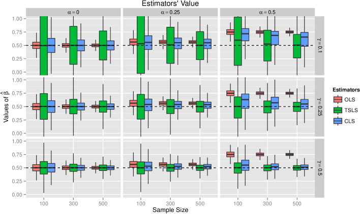
Figure 2: Monte Carlo distributions of the estimators’ values under three different levels of confounding, $\alpha=\operatorname{Cor}(X_{i},U_{i})$; and for three different levels of instrument’s strength, $\gamma=\operatorname{Cor}(X_{i},Z_{i})$. In each panel, the sample size varies between $n=100$ and $n=500$. We here compare the OLS, TSLS and CLS estimators with respect to the true parameter $\beta=1/2$, whose value is indicated by a dashed line. These simulations are based on $10^{5}$ iterations for each scenario. The boxplots are here centered at the median, and the upper and lower hinges correspond to the first and third quartiles.

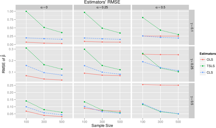
Figure 3: Monte Carlo estimates of the root mean squared errors (RMSEs) of the three estimators of interest under the simulation scenarios described in figure 2. As predicted, the RMSE of the proposed CLS method strikes a trade-off between its two constituent estimators. Indeed, under small $\alpha$, the CLS’s RMSE tends towards the RMSE of the OLS estimator; whereas under large $\gamma$, it tends towards the RMSE of the TSLS estimator.

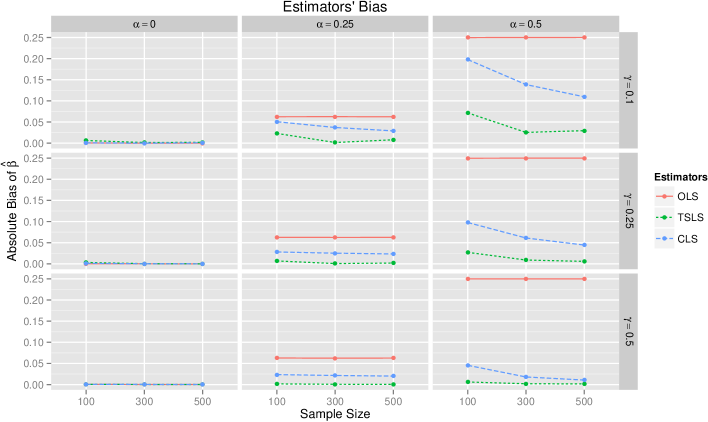
Figure 4: Monte Carlo estimates of the absolute value of the bias of the three estimators of interest, under the simulation scenarios described in figure 2. Observe that the three estimators exhibit no bias, when no confounding is present. That is, the OLS estimator exhibits less bias, when $\alpha=\operatorname{Cor}(X_{i},U_{i})$ is low. Also, note that the finite-sample bias of the TSLS estimator tends to diminish with large sample sizes. This behavior is especially visible for large $\alpha$’s.

Figure 5: Monte Carlo standard deviation of the three estimators under scrutiny, under the scenarios described in figure 2. By corollary 1, the variance of the OLS estimator is always smaller than its competitors, as verified in these simulations. Moreover, observe that the variance of the TSLS estimator increases as the strength of the instrument, $\gamma=\operatorname{Cor}(X_{i},Z_{i})$, decreases.

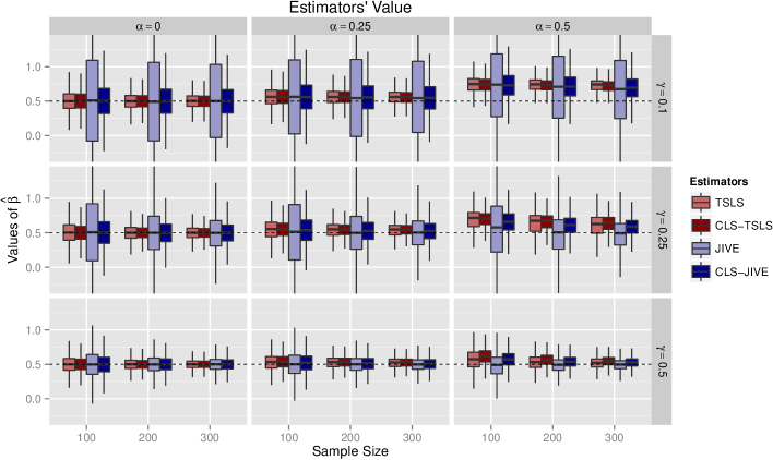
Figure 6: Comparison of the TSLS and JIVE estimators with their CLS counterparts, using $l=10$ uncorrelated instruments, whose multiple correlation with the outcome is given by $\gamma$, and with $\alpha$ measuring the strength of bias, as in Model I. Data have been simulated using Model II from section 4.2. The bootstrap estimate of $\pi_{n}$ for the CLS-JIVE is based on $B=100$ resamples, as described in section 3.2 on bootstrap CLS estimation. All scenarios have been repeated over $10^{5}$ Monte Carlo iterations.

Figure 7: Monte Carlo estimates of the absolute value of the bias of four estimators of interest for Model II with $l=10$ uncorrelated instruments, whose multiple correlation with the outcome is given by $\gamma$, and with the strength of the bias being denoted by $\alpha$. As in figure 6, all scenarios have been repeated over $10^{5}$ Monte Carlo iterations.

4.2 Simulation Model II

We extend Model I to the case of several valid instruments. For convenience, these instruments are assumed to be uncorrelated. The second-level equation is taken to be identical to the second-level equation in equation (15). The first-level equation, by contrast, now includes a vector of instruments, such that

$$x_{i}=\text{\bf{z}}_{i}\bm{\lambda}+u_{i}\alpha+\delta_{i},$$ (17)

for every $i=1,\ldots,n$; and where $\text{\bf{z}}_{i}:=(z_{i1},\ldots,z_{il})$ is a row vector of $l$ uncorrelated instruments. The strengths of each of these instruments are controlled by a column vector of parameters denoted by $\bm{\lambda}:=(\lambda_{1},\ldots,\lambda_{l})^{\prime}$. We here assume that the $\lambda_{j}$’s are held constant such that $\lambda_{j}:=\lambda$, for every $j=1,\ldots,l$. As for Model I, we fix $\operatorname{\mathbb{V}ar}(Y_{i})=\operatorname{\mathbb{V}ar}(X_{i})=1$, and generate the $Z_{ij}$’s and the $U_{i}$’s from a standard normal distribution, with $\sigma_{z}^{2}:=1$ and $\sigma^{2}_{u}:=1$, respectively. The formula for the error variance of the second-level equation, $\sigma^{2}_{\varepsilon}(\alpha)$, is identical to the one used in Model I.

The error variance for the first-level equation, denoted by $\sigma^{2}_{\delta}$, is also controlled by a parameter $\gamma$, which is here defined to be the coefficient of multiple correlation between each $X_{i}$ and the $i^{\text{th}}$ vector of $Z_{ij}$’s. As before, using the Bienaymé formula, the variance of each $X_{i}$ can be expanded as follows,

$$\operatorname{\mathbb{V}ar}(X_{i})=\sum_{j=1}^{l}\lambda^{2}_{j}\operatorname{\mathbb{V}ar}(Z_{ij})+\alpha^{2}\operatorname{\mathbb{V}ar}(U_{i})+\operatorname{\mathbb{V}ar}(\delta_{i}),$$

which simplifies to $\operatorname{\mathbb{V}ar}(X_{i})=l\lambda^{2}+\alpha^{2}+\sigma^{2}_{\delta}$, by our choice of variances for the $Z_{ij}$’s and $U_{i}$’s. When specifying $\operatorname{\mathbb{V}ar}(X_{i})=1$, this gives $\sigma^{2}_{\delta}(\alpha,\gamma,l)=1-(l\lambda^{2}+\alpha^{2})$, and moreover, when enforcing the positiveness of $\sigma^{2}_{\delta}$, we obtain $\lambda<\sqrt{(1-\alpha^{2})/l}$. Next, if we choose $\lambda:=\gamma/\sqrt{l}$, then the parameter $\gamma$ can be seen to correspond to the multiple correlation coefficient between each $X_{i}$ and the $i^{\text{th}}$ vector of $Z_{ij}$’s. Indeed, we have $\gamma^{2}=\text{\bf{r}}^{T}\text{\bf{R}}^{-1}\text{\bf{r}}$, in which $\text{\bf{r}}:=(r_{xz},\ldots,r_{xz})^{\prime}$, with $r_{xz}:=\operatorname{Cor}(X_{i},Z_{ij})=\gamma$; and where R is the correlation matrix of the $i^{\text{th}}$ vector of $Z_{ij}$’s, such that $R_{ab}:=\operatorname{Cor}(Z_{ia},Z_{ib})$, for every $a,b=1,\ldots,l$. Thus, as in Model I, we again obtain the upper bound, $\gamma<\sqrt{1-\alpha^{2}}$, as well as $\sigma_{\delta}^{2}(\alpha,\gamma)=1-(\gamma^{2}+\alpha^{2})$.

4.3 Monte Carlo Summary Statistics

We evaluate the finite-sample performance of the estimators of interest by comparing the Monte Carlo estimates of three different population statistics. For every candidate estimator, $\bm{\beta}_{n}^{{\dagger}}$, its Monte Carlo distribution is given by the following empirical distribution function (EDF), $\widehat{F}(b):=T^{-1}\sum_{t}\mathcal{I}\{\bm{\beta}_{nt}^{{\dagger}}\leq b\}$, where $\mathcal{I}\{f_{t}\}$ denotes the indicator function taking a value of one, if $f_{t}$ is true, and zero otherwise. For each simulation scenario, we draw $T:=10^{5}$ realizations from the two models described in sections 4.1 and 4.2.

Using these simulated samples, we compute the Monte Carlo estimates of the bias, variance, and MSE; denoted by $\operatorname{\mathbb{B}ias}_{\widehat{F}}(\bm{\beta}_{n}^{{\dagger}})$, $\operatorname{\mathbb{V}ar}_{\widehat{F}}(\bm{\beta}_{n}^{{\dagger}})$, and $\operatorname{MSE}_{\widehat{F}}(\bm{\beta}_{n}^{{\dagger}})$, respectively. In figure 2, we have reported the Monte Carlo distribution of the three estimators of interest under $T$ simulations from model I; whereas in figures 3, 4, and 5 we have reported the Monte Carlo MSE, squared bias, and variance, respectively. The quantities in these three figures have been square-rooted in order to facilitate the comparison of these statistics with the estimators’ values in figure 2. Similarly, in figure 6, we have reported the Monte Carlo distributions of the TSLS, JIVE, as well as their CLS counterparts; with the Monte Carlo estimates of their absolute value bias being described in figure 7.

4.4 Results for Model I (Single Instrument)

The behavior of the CLS was found to be mainly controlled by the strength of the instrument, $Z$. When the instrument was strongly correlated with the predictor $X$ –that is, for large values of $\gamma=\operatorname{Cor}(X_{i},Z_{i})$; the values of the CLS estimator were close to the ones of the TSLS estimators, as can be observed in the last row of figure 2. By contrast, when the instrument was weak –that is, for small values of $\gamma$, the values of the CLS estimator were closer to the ones of the OLS estimator, as can be seen in the first row of figure 2.

Proposition 3 stated that the MSEs of the OLS and TSLS estimators are bounded below by the MSE of the CLS estimator when the true proportion $\pi_{n}$ is known. These Monte Carlo simulations appear to support a partial analog of this result when $\pi_{n}$ is evaluated from the data. Indeed, on one hand, figure 3 shows that the MSE of the OLS estimator tends to be smaller than the MSE of the CLS estimator, when no confounding is present; thereby showing that proposition 3 does not strictly hold when $\pi_{n}$ is estimated from the data. However, on the other hand, one can also observe from figure 3 that the Monte Carlo MSE of the CLS estimator is smaller than or equal to the one of the TSLS estimator under all considered scenarios. Thus, it seems that a weaker version of proposition 3 may hold for estimated $\pi_{n}$, which would solely pertain to a comparison between the behavior of the CLS and TSLS estimators. In particular, observe that for strong instruments (i.e. for large values of $\gamma$), the CLS estimator behave as well as the TSLS estimator, whereas for weak instruments (i.e. small values of $\gamma$), the CLS estimator outperforms the TSLS estimator.

The behavior of these estimators can be better understood by separately considering their bias and variance. In figures 4 and 5, we have respectively reported the Monte Carlo estimates of the bias and variance of the OLS, TSLS and CLS estimators. Naturally, the bias of the three estimators tends to increase with the strength of the confounder, which is controlled by $\alpha=\operatorname{Cor}(X_{i},U_{i})$. In particular, the bias of the OLS estimator becomes larges as $\alpha$ increases. By contrast, the bias of the TSLS estimator remains small for every value of $\alpha$. In fact, as stated in Corollary 1(i), the bias of the OLS estimator is bounded from below by the bias of the TSLS estimator. Moreover, the finite-sample bias of the TSLS estimator can also be observed to decrease as the sample size increases. As predicted, the bias of the CLS estimator is comprised between the ones of the two other estimators; and the bias of the CLS estimator approaches the one of the TSLS estimator, as the strength of the instrument increases.

Figure 5 describes the behavior of the variance of the estimators of interest under our various simulation scenarios. The variance of the three estimators tends to decrease as the sample size increases. This downward trend is especially noticeable for the TSLS estimator, which exhibits a high level of variability, when the instrument is weak (i.e. for small values of $\gamma$). As predicted by Corollary 1(ii), the variance of the TSLS estimator can be observed to be bounded from below by the variance of the OLS estimator. In the presence of weak instruments, the CLS estimator’s variance is close to the one of the OLS estimator. As $\gamma$ increases, however, the variance of the CLS estimator converges to the one of the TSLS estimator.

4.5 Results for Model II (Multiple Instruments)

Our second set of simulations aimed to assess whether the use of an estimator possessing better finite-sample properties could be incorporated into the CLS framework. In figure 4, we have already seen that the TSLS estimator suffers from a substantial finite-sample bias. This was found to be especially the case when the instruments of interest are comparatively weak, and the bias is large. In particular, previous authors have shown that the TSLS estimator’s bias tends to be especially large, when several instruments are used (Angrist et al., 1995). This limitation of the TSLS estimator has been addressed in the literature by the introduction of the JIVE, which was described in section 3.1. This second set of simulations is thus based on $l=10$ uncorrelated instruments, and allow us to compare the relative merits of using either the TSLS estimator or the JIVE within the CLS framework. Consequently, we will refer to using the TSLS and using the JIVE as unbiased estimators within the CLS, as the CLS-TSLS and CLS-JIVE estimators, respectively.

As predicted, the JIVE performs better than the TSLS estimator, when used in conjunction with strong instruments, and in the presence of a substantial amount of confounding (i.e. $\alpha\geq 0.25$), as can be seen from figures 6 and 7. Note, however, that for weak instruments (i.e. when the multiple correlation coefficient is $\gamma=0.1$), the JIVE’s variance is very large. The TSLS estimator should therefore be favored under these scenarios, if one’s choice of estimator is motivated by a desire to minimize the MSE.

The benefits of using the JIVE translate into corresponding improvements when using the CLS-JIVE. This relationship is especially visible when considering the bottom right panel of figure 7. Under a set of strong instruments (i.e. with a large multiple correlation coefficient $\gamma$), and under a substantial amount of confounding (i.e. large $\alpha$); one can observe that the JIVE has a smaller finite-sample bias than the TSLS estimator. Similarly, under the same scenario, the CLS-JIVE has a correspondingly smaller finite-sample bias than the CLS-TSLS estimator. This improvement in the CLS-JIVE was particularly remarkable, because the proportion parameter, $\widehat{\pi}_{n}$, was estimated using only $B=100$ bootstrap samples. Thus, it appears that a relatively small number of resampling is sufficient to produce a CLS-JIVE estimator that outperforms the CLS-TSLS estimator. One may therefore conjecture that the CLS framework could be used in conjunction with other asymptotically unbiased estimators, even when the proportion parameter is not available in closed-form.

5 Applications to Econometrics

Our proposed methods have been applied to a re-analysis of a classic data set in econometrics, originally published by Angrist and Krueger (1991), which aimed to relate educational attainment with earnings. This particular study has been the subject of numerous replications and re-analysis, and therefore provides us with a well-known example for evaluating the performance of CLS estimation in a real-world data set.

5.1 Quarter-of-Birth as Instrument

Angrist and Krueger (1991) reported a small but persistent seasonal pattern of educational attainment over several decades between the 1920s and the 1950s. They observed that two discrepant regulations in the United States during that period have led to a ‘natural experiment’, in which individual differences in completed years of education could be predicted by an individual’s season of birth. On one hand, nationwide school-entry requirements controlled the age at which a given child began school. Indeed, at that period in the US, all children were expected to reach six years of age by the first of January of their first year at school. Thus, children born early in the year were likely to be older than their peers in the same class. On the other hand, state-specific compulsory schooling laws solely required pupils to remain in school until their sixteenth birthday. Therefore, pupils born in the first quarters of the year, wishing to leave school early, could do so at an earlier stage than their peers born later in the year.

These two regulations –school-entry requirements, and compulsory schooling laws– therefore conspired to enable children born in the early quarters of the year to complete a smaller number of years of education, if they were so inclined. Crucially, Angrist and Krueger (1991) highlights that the randomness of an individual’s birth date is unlikely to be related to other events in an individual’s life; thereby precluding quarter-of-birth from being a significant predictor of an individual’s revenue later in life. Thus, quarter-of-birth could be argued to constitute a legitimate instrument for education attainment, fulfilling the exclusion criterion, in the sense that it is not directly related to earnings. Note, however, that some authors have disputed the validity of quarter-of-birth as an instrument for education (Bound and Jaeger, 1996).

Figure 8: Graphical representation of the IV model described in equations (18) and (19), composed of a vector of endogenous variables, $X_{1}$, and a vector of exogenous variables $X_{2}$. This graph corresponds to a two-level system of equations composed of $Y=X_{1}\bm{\beta}_{1}+X_{2}\bm{\beta}_{2}+U\alpha+\varepsilon$, and $X_{1}=Z_{1}\bm{\Gamma}_{1}+X_{2}\bm{\Gamma}_{2}+U\alpha+\delta$. This model can be seen to be a generalization of the simpler model described in figure 1.

Table 1: Replications and extensions of the IV analysis in Angrist and Krueger (1991).

Covariates ($X_{2}$)		OLS	TSLS	JIVE	CLS-TSLS
A.a	Estimator:	0.0802	0.0769	0.0755	0.0800
	Std. Error:	(0.0004)	(0.0150)	(0.0210)	(0.0126)
	Proportion:	–	–		(0.95)
B.b	Estimator:	0.0802	0.1398	-0.1276	0.1254
	Std. Error:	(0.0004)	(0.0334)	(1.7233)	(0.0317)
	Proportion:	–	–		(0.24)
C.c	Estimator:	0.0701	0.0669	0.0650	0.0700
	Std. Error:	(0.0004)	(0.0151)	(0.0234)	(0.0097)
	Proportion:	–	–		(0.96)
D.d	Estimator:	0.0701	0.1065	0.0224	0.0899
	Std. Error:	(0.0004)	(0.0334)	(2.1380)	(0.0235)
	Proportion:	–	–		(0.46)

• This only includes ten dummies for the years of birth.

• This includes years of birth, and age with the exclusion of the 1929 dummy.

• Covariates include years of birth, and some extraneous covariates described in the text.

• Covariates are years of birth, age, and other extraneous covariates, with the exclusion of the 1929 dummy.

5.2 Model with Extraneous Covariates

The model used by Angrist and Krueger (1991) generalizes the IV model described in sections 2.1 and 2.2. Here, the vector of $k$ predictors, $X$, is partitioned into $k_{1}$ endogenous variables denoted by $X_{1}$, and $k_{2}$ exogenous variables denoted by $X_{2}$. In Angrist and Krueger’s model, the sole endogenous variable of interest is the completed years of education of each subject. Therefore, we have $k_{1}=1$. The outcome variable, $Y$, which represents the log-transformed weekly wage in dollars of each subject, is then modelled as follows,

$$Y=X_{1}\bm{\beta}_{1}+X_{2}\bm{\beta}_{2}+\varepsilon,$$ (18)

where $\bm{\beta}_{1}$ and $\bm{\beta}_{2}$ are column vectors of dimension $k_{1}$ and $k_{2}$, respectively. The endogeneity of $X_{1}$ leads to the use of a row vector of instruments, $Z_{1}$, of dimension $1\times l_{1}$, here denoting a set of dummy variables for the interactions between quarters and years of birth. These instruments are combined with the $k_{2}$ exogenous variables from the second-level equation in order to produce the following first-level equation,

$$X=Z_{1}\bm{\Gamma}_{1}+X_{2}\bm{\Gamma}_{2}+\delta;$$ (19)

where $\bm{\Gamma}_{1}$ and $\bm{\Gamma}_{2}$ are vectors of parameters of order $l_{1}\times k$ and $k_{2}\times k$, respectively; where $k:=k_{1}+k_{2}$. A graphical representation of this model is given in figure 8.

In matrix notation, given a sample of $n$ subjects, this model can be expressed with respect to an $n$-dimensional column vector of error terms, $\bm{\varepsilon}$, for the first-level equation; and a matrix, D, of error terms of order $n\times k_{1}$ for the second-level equation. Altogether, we thus have the following linear system,

y $$=\text{\bf{X}}_{1}\bm{\beta}_{1}+\text{\bf{X}}_{2}\bm{\beta}_{2}+\bm{\varepsilon},$$

X $$=\text{\bf{Z}}_{1}\bm{\Gamma}_{1}+\text{\bf{X}}_{2}\bm{\Gamma}_{2}+\text{\bf{D}}.$$

Moreover, we can construct the following block matrices, $\text{\bf{X}}:=[\text{\bf{X}}_{1}\;\text{\bf{X}}_{2}]$ and $\text{\bf{Z}}:=[\text{\bf{Z}}_{1}\;\text{\bf{X}}_{2}]$ that are of order $n\times k$ and $n\times l$, respectively; in which we have used $k:=k_{1}+k_{2}$ and $l:=l_{1}+k_{2}$. In addition, we also define the vectors of parameters $\bm{\beta}:=[\bm{\beta}_{1}^{T}\;\bm{\beta}_{2}^{T}]^{T}$ and $\bm{\Gamma}:=[\bm{\Gamma}_{1}^{T}\;\bm{\Gamma}_{2}^{T}]^{T}$, of order $k\times 1$ and $l\times k$, respectively. Equipped with these block matrices, we can immediately recover the standard TSLS estimator formula described in section 2.2. It also follows that this model is well-identified whenever $l_{1}\geq k_{1}$ is satisfied, as in the model at hand.

5.3 Results of the Re-analysis

The results described in table 4 of Angrist and Krueger (1991) have been replicated and extended. In this portion of their analysis, Angrist and Krueger have considered the cohort of men born between 1920 and 1929. This constitutes a sample of $n=247,199$ subjects. All data are here based on the 1970 US census. Using the notation introduced in equations (18) and (19), the outcome variable, $Y$, is defined as the mean log-transformed weekly wages; the endogenous variable, $X_{1}$, is the number of completed years of education; and the instrument, $Z_{1}$, is composed of a vector of interaction terms between quarter-of-year dummies and year-of-birth dummies, totalling 40 different instruments.

In addition, the authors have also considered different sets of exogenous covariates, denoted by $X_{2}$ in equations (18) and (19). The choice of exogenous covariates has been reported as covariate scenarios A to D in table 1. All scenarios include ten dummy variables for each year of birth, except scenarios B and D, in which the 1929 dummy variable has been removed due to multicollinearity, following Angrist and Krueger (1991). In scenarios B and D, this is supplemented by an age covariate. (Note that we have not included age squared in this analysis as was conducted in Angrist and Krueger (1991), since age and age squared were found to be almost perfected correlated.) Finally, scenarios C and D include some further dummy variables for race, marital status, eight different regions of residence, and whether or not the subjects were primarily located in a standard metropolitan statistical area (SMSA).

For scenarios A and C, the OLS and TSLS columns in table 1 are exact replicates of the results described in Angrist and Krueger (1991). The values and standard errors for these estimators are slightly different under scenarios B and D, due to the non-inclusion of age squared in the present analysis. The variance of the CLS estimator was computed using the bootstrap, as described in section 2.6. As expected, one can observe that the CLS strikes a balance between the OLS and the TSLS estimators, such that for all four scenarios, the value of the CLS is comprised between the one of the OLS and the one of the TSLS. The value taken by the estimate of the proportion parameter has also been reported. By comparing scenarios A and C with scenarios B and D in table 1, it can be seen that the inclusion (resp. non-inclusion) of the age variable leads to a decrease (resp. increase) in the value of $\widehat{\pi}_{n}$.

Thus, this re-analysis suggests that while the use of quarter-of-birth as an IV for education may be justified when age is included as a supplementary exogenous variable in the analysis; it appears that an estimator closer to the OLS is sufficient, when the age variable is not included. The JIVE and its CLS counterpart have also been reported for comparison. The behavior of these two estimators is comparable to the one of the TSLS and CLS-TSLS estimators. Note that for computational convenience, the variances of the CLS estimators and the proportion parameter of the CLS-JIVE have been here estimated using bootstraps based on solely $10^{2}$ resamples. This real data analysis thus demonstrates that a small number of bootstrap samples suffices to produce reasonable estimates of the standard errors of the CLS estimators.

6 Conclusions

In this paper, we have shown that different IV and non-IV estimators can be the object of convex combinations, and the proportion parameters of these combinations can be consistently estimated from the data. Such CLS estimators are therefore particularly attractive, since they automatically down-weight the influence of weak instruments, when these are not expected to lead to a large reduction in bias. Moreover, this inferential framework bears some similarities with the Hausmann test. Theoretically, our proposed estimator minimizes an empirical MSE over a restricted class of estimators, consisting of all the possible convex combinations of the OLS and TSLS estimators. We have also seen the TSLS estimator in the definition of the CLS can be replaced by other estimators such as the JIVE.

For finite $n$, the moments of the TSLS estimator and other $k$-class estimators need not exist, as demonstrated by Kinal (1980). It is common in such situations to assume that at least three instruments are present. This condition ensures that the first two moments of the estimators under scrutiny exist; and the first two moments of the OLS and TSLS estimators are needed to compute our proposed empirical estimator of the MSE. However, note that, asymptotically, all moments exist and that, theoretically, this strategy can thus be applied to any number of instruments. Indeed, irrespective of the number of instruments used, every CLS estimator is guaranteed to be asymptotically consistent. Observe that a similar issue arises for all IV models, in the sense that such models are only asymptotically identifiable. In the present case, our proposed estimation procedure only possesses asymptotic first and second moments. However, just as finite-sample non-identifiability is not a point of concern for the use of IV methods in practice, the reliance of the CLS framework on asymptotic moments does not constitute a significant hindrance to the general application of this method.

The interpretation of the combination of several estimators such as the OLS and TSLS estimators relies on the assumption of effect homogeneity [REFs needed]. That is, we are assuming that the causal effect is identical for all subpopulations. This is a strong assumption, which needs not hold in practice. Thus, further research will be needed to clarify the assumptions required for employing the CLS, when effect homogeneity is not expected to hold. Indeed, in such cases, the OLS and the TSLS estimators may represent the local treatment effects in different subpopulations. Therefore, the resulting convex combination of such estimators may be difficult to interpret. Additional assumptions may be required to ensure that the different estimators of interest are sufficiently comparable to be combined in this fashion.

Observe that the estimators utilized to produce the CLS estimator do not need to share the same data. Indeed, when constructing a combination of the OLS and TSLS estimators, only the TSLS estimator relies on the instrument, $Z$. Thus, one may also consider how such a framework could be extended to other modelling strategies, such as mixed-effects models for longitudinal models (see Wooldridge, 2002). Similarly, this method could also be extended to models including measurement errors. Calibrated regression is often used in conjunction with explanatory variables, in order to diminish the effect of measurement error. In such cases, the resulting combination utilizes estimators based on distinct data sets. In addition, recall that of the theoretical results derived in this paper are relying one the assumption that the instruments under scrutiny are valid, in the sense that (A4) is assumed to hold. The consequences of relaxing this assumption are difficult to anticipate, and further research should certain consider such situations, as has been done by previous authors in the case of the TSLS estimator (Jackson and Swanson, In press).

Thus far, we have combined the OLS estimator with either the TSLS estimator or the JIVE. Observe, however, that we are not restricted to choosing the OLS as a reference estimator. Within the bootstrap CLS framework described in section 3.2, one could also choose to combine the TSLS and the JIVE, for instance. In general, any pair of estimators could be the object of a convex combination. For such a combination to be useful, it suffices that these estimators are ordered in terms of bias and variance, as in the canonical case of the OLS and TSLS estimators given in proposition 1. Another natural theoretical extension of the current work would be to derive a central limit theorem for the CLS estimator. This would allow researchers to obtain approximate confidence intervals for the CLS estimator, using normal asymptotic theory. Such a central limit theorem would also enable the construction of adequate statistical tests for evaluating whether or not the values of individual parameters are statistically significant. Such extensions are not expected to be too arduous, since under the assumptions stated in this paper, the CLS estimator is consistent; and moreover, estimators such as the TSLS or JIVE are known to be asymptotically normally distributed under standard assumptions.

Appendix A Proofs of Propositions

Proof of Proposition 1.

The proof of (i) immediately follows from the definition of the empirical bias in equation (8), which implies that the empirical bias of the TSLS estimator is identically zero, for every realization. The proof of (ii) can be conducted in two steps. Firstly, one can show that for every pair of matrices X and $\widehat{\text{\bf{X}}}:=\text{\bf{H}}_{z}\text{\bf{X}}$, we have

$$\text{\bf{X}}^{\prime}\text{\bf{X}}\succeq\widehat{\text{\bf{X}}}{}^{\prime}\widehat{\text{\bf{X}}}.$$ (20)

Observe that we have the following equivalence due to the symmetry of $\text{\bf{H}}_{z}$,

$$\widehat{\text{\bf{X}}}{}^{\prime}\text{\bf{X}}=(\text{\bf{H}}_{z}\text{\bf{X}})^{\prime}\text{\bf{X}}=\text{\bf{X}}^{\prime}\text{\bf{H}}_{z}\text{\bf{X}}=\text{\bf{X}}^{\prime}\widehat{\text{\bf{X}}}.$$ (21)

Secondly, the inner product of $\widehat{\text{\bf{X}}}$ can also be simplified using the idempotency of $\text{\bf{H}}_{z}$, such that

$$\text{\bf{X}}^{\prime}\widehat{\text{\bf{X}}}=\text{\bf{X}}^{\prime}\text{\bf{H}}_{z}\text{\bf{X}}=\text{\bf{X}}^{\prime}\text{\bf{H}}_{z}\text{\bf{H}}_{z}\text{\bf{X}}=\widehat{\text{\bf{X}}}{}^{\prime}\widehat{\text{\bf{X}}}.$$ (22)

Then, expanding the dot product of $\text{\bf{X}}-\widehat{\text{\bf{X}}}$, and applying equalities (21) and (22), we obtain

$$(\text{\bf{X}}-\widehat{\text{\bf{X}}})^{\prime}(\text{\bf{X}}-\widehat{\text{\bf{X}}})=\text{\bf{X}}^{\prime}\text{\bf{X}}-2\text{\bf{X}}^{\prime}\widehat{\text{\bf{X}}}+\widehat{\text{\bf{X}}}{}^{\prime}\widehat{\text{\bf{X}}}=\text{\bf{X}}^{\prime}\text{\bf{X}}-\widehat{\text{\bf{X}}}{}^{\prime}\widehat{\text{\bf{X}}}.$$

Observe that the dot product, $(\text{\bf{X}}-\widehat{\text{\bf{X}}})^{\prime}(\text{\bf{X}}-\widehat{\text{\bf{X}}})$, is a Gram matrix, and therefore it is necessarily positive semi-definite. Consequently, this implies that

$$\text{\bf{X}}^{\prime}\text{\bf{X}}-\widehat{\text{\bf{X}}}{}^{\prime}\widehat{\text{\bf{X}}}=(\text{\bf{X}}-\widehat{\text{\bf{X}}})^{\prime}(\text{\bf{X}}-\widehat{\text{\bf{X}}})\succeq\bm{0},$$

and hence $\text{\bf{X}}^{\prime}\text{\bf{X}}\succeq\widehat{\text{\bf{X}}}{}^{\prime}\widehat{\text{\bf{X}}}$, by the definition of the positive semidefinite order.

Next, observe that the estimates of the error variances under the OLS and TSLS estimation procedures are defined as

$$(n-k)\widehat{\sigma}^{2}_{n} :=(\text{\bf{y}}-\text{\bf{X}}\widehat{\bm{\beta}}_{n})^{\prime}(\text{\bf{y}}-\text{\bf{X}}\widehat{\bm{\beta}}_{n})$$

$$\leq(\text{\bf{y}}-\text{\bf{X}}\widetilde{\bm{\beta}}_{n})^{\prime}(\text{\bf{y}}-\text{\bf{X}}\widetilde{\bm{\beta}}_{n})=:(n-k)\widetilde{\sigma}^{2}_{n},$$

where the inequality follows from the optimality of the OLS; and therefore,

$$\widehat{\sigma}^{2}_{n}(\text{\bf{X}}^{\prime}\text{\bf{X}})^{-1}\preceq\;\widetilde{\sigma}^{2}_{n}(\widehat{\text{\bf{X}}}{}^{\prime}\widehat{\text{\bf{X}}})^{-1},$$

since assumption (A6) guarantees that both sides are invertible. ∎

Proof of Corollary 1.

For inequality (i), observe that the empirical bias of the TSLS estimator is identically zero for every realization and every $n$. Moreover, by equation 8, the empirical bias of the OLS estimator is given by

$$\widehat{\operatorname{\mathbb{B}ias}}{}^{2}(\widehat{\bm{\beta}}_{n})=(\widehat{\bm{\beta}}_{n}-\widetilde{\bm{\beta}}_{n})(\widehat{\bm{\beta}}_{n}-\widetilde{\bm{\beta}}_{n})^{\prime}\succeq\bm{0},$$

since the LHS is a Gram matrix, and is therefore positive semidefinite for every realization. Since it holds for every $n$, this positive semidefiniteness is preserved in the limit. Moreover, the inequality in (ii) immediately follows from the fact that the variances of these two estimators converge to the zero matrix. ∎

Proof of Proposition 2.

The optimal value of $\pi_{n}$ can be found by minimizing the criterion of interest, which will be denoted by $f(\pi):=\operatorname{MSE}(\bar{\bm{\beta}}_{n}(\pi))$. For expediency, we will expand this criterion as was done in equation (10) such that

$$\operatorname{tr}f(\pi)=\operatorname{tr}(\pi^{2}M_{1}+2\pi(1-\pi)C+(1-\pi)^{2}M_{2}),$$

with $M_{1}:=\operatorname{MSE}(\widehat{\bm{\beta}}_{n})$, $C:=\operatorname{CSE}(\widehat{\bm{\beta}}_{n},\widetilde{\bm{\beta}}_{n})$, and $M_{2}:=\operatorname{MSE}(\widetilde{\bm{\beta}}_{n})$; and where recall that $\widehat{\bm{\beta}}_{n}$ and $\widetilde{\bm{\beta}}_{n}$ denote the OLS and TSLS estimators, respectively. Since the derivative is a linear operator, it commutes with the trace, and we obtain

$$\operatorname{tr}(\partial f/\partial\pi)=2\pi\operatorname{tr}(M_{2}-2C+M_{1})-2\operatorname{tr}(M_{2}-C),$$

Setting this expression to zero, yields $\pi_{n}:=\operatorname{tr}(M_{2}-C)/\operatorname{tr}(M_{2}-2C+M_{1})$, as required. Naturally, this minimization holds for every choice of $n$, thereby proving the first part of proposition 2.

In addition, one can show that this minimizer is unique by performing a second derivative test, such that we obtain

$$\operatorname{tr}(\partial^{2}f/\partial\pi^{2})=2\operatorname{tr}(M_{1}-2C+M_{2}).$$ (23)

Since by assumption, the random vectors, $\widehat{\bm{\beta}}_{n}$ and $\widetilde{\bm{\beta}}_{n}$, are elementwise squared-integrable, the components, $\mathbb{E}[(\widehat{\beta}_{nj}-\beta_{j})^{2}]$, of $M_{1}$ are finite for every $j=1,\ldots,k$. Hence, using the linearity of the trace, the MSE of $\widehat{\bm{\beta}}_{n}$ can be treated as a sum of real numbers, thereby yielding the $L^{2}$-norm on $\mathbb{R}^{k}$, such that

$$\big{(}\operatorname{tr}\operatorname{MSE}(\widehat{\bm{\beta}}_{n})\big{)}^{1/2}=\bigg{(}\sum_{j=1}^{k}\mathbb{E}\!\left[(\widehat{\beta}_{nj}-\beta_{j})^{2}\right]\bigg{)}^{1/2}=:||\widehat{\bm{\beta}}_{n}-\bm{\beta}||.$$

The latter quantity will be referred to as the root (trace) MSE of $\widehat{\bm{\beta}}_{n}$, and will be denoted by RMSE.

By the same reasoning, it can be shown that $C$ and $M_{2}$ corresponds to the inner product, $\langle\widehat{\bm{\beta}}_{n}-\bm{\beta},\widetilde{\bm{\beta}}_{n}-\bm{\beta}\rangle$, and the squared norm, $||\widetilde{\bm{\beta}}_{n}-\bm{\beta}||^{2}$, on $\mathbb{R}^{k}$. Thus, equation (23) can now be re-expressed as follows,

$$\operatorname{tr}(\partial^{2}f/\partial\pi^{2})=2\Big{(}||\widehat{\bm{\beta}}_{n}-\bm{\beta}||^{2}-2\langle\widehat{\bm{\beta}}_{n}-\bm{\beta},\widetilde{\bm{\beta}}_{n}-\bm{\beta}\rangle+||\widetilde{\bm{\beta}}_{n}-\bm{\beta}||^{2}\Big{)}.$$

The Cauchy-Schwarz inequality can here be invoked to produce an upper bound on the cross-term in the latter equation,

$$\langle\widehat{\bm{\beta}}_{n}-\bm{\beta},\widetilde{\bm{\beta}}_{n}-\bm{\beta}\rangle\leq||\widehat{\bm{\beta}}_{n}-\bm{\beta}||\cdot||\widetilde{\bm{\beta}}_{n}-\bm{\beta}||.$$

It then suffices to complete the square in order to obtain the following lower bound,

$$\operatorname{tr}(\partial^{2}f/\partial\pi^{2})\geq 2\Big{(}||\widehat{\bm{\beta}}_{n}-\bm{\beta}||-||\widetilde{\bm{\beta}}_{n}-\bm{\beta}||\Big{)}^{2}\geq 0,$$

for every $n$, and where equality only holds when the RMSEs of $\widehat{\bm{\beta}}_{n}$ and $\widetilde{\bm{\beta}}_{n}$ are identical, as required. ∎

Proof of Proposition 4.

Firstly, observe that the stochastic convergence of $\bar{\bm{\beta}}_{n}(\pi)$ to $\pi\widehat{\bm{\beta}}+(1-\pi)\widetilde{\bm{\beta}}$ is immediate from the convergence of $\widehat{\bm{\beta}}_{n}$ and $\widetilde{\bm{\beta}}_{n}$ to their respective limits, $\widehat{\bm{\beta}}$ and $\widetilde{\bm{\beta}}$. Naturally, this holds for every $\pi\in[0,1]$.

Secondly, recall that the empirical MSE of $\bar{\bm{\beta}}_{n}(\pi)$ can be decomposed into a variance and a bias term, as in equation (12), such that for every $\pi$, we have

$$\widehat{\operatorname{MSE}}(\bar{\bm{\beta}}_{n}(\pi))=\widehat{\operatorname{\mathbb{V}ar}}(\bar{\bm{\beta}}_{n}(\pi))+\widehat{\operatorname{\mathbb{B}ias}}{}^{2}(\bar{\bm{\beta}}_{n}(\pi)).$$

The variances of both the OLS and TSLS estimators are known to converge to zero. Moreover, the bias of the TSLS estimator is also known to converge to zero, and this can be seen to be also true for the cross-bias term. Thus, the stochastic limit of $\widehat{\operatorname{MSE}}(\bar{\bm{\beta}}_{n}(\pi))$ reduces to the weighted limit of the empirical bias of the OLS estimator, $\pi^{2}\widehat{\operatorname{\mathbb{B}ias}}{}^{2}(\widehat{\bm{\beta}}_{n})$. Using the consistency of the TSLS estimator, this latter term satisfies

$$\operatornamewithlimits{plim}_{n\to\infty}\widehat{\operatorname{\mathbb{B}ias}}(\widehat{\bm{\beta}}_{n})=\operatornamewithlimits{plim}_{n\to\infty}(\widetilde{\bm{\beta}}_{n}-\widehat{\bm{\beta}}_{n})=\operatorname{\mathbb{B}ias}(\widehat{\bm{\beta}})=(\bm{\beta}-\widehat{\bm{\beta}}),$$

since $\widehat{\bm{\beta}}_{n}\stackrel{{\scriptstyle p}}{{\longrightarrow}}\widehat{\bm{\beta}}$, and $\widehat{\bm{\beta}}=\lim_{n}\mathbb{E}[\widehat{\bm{\beta}}_{n}]$; which is the true bias of the OLS estimator. The result then follows by using the continuous mapping theorem. ∎

Proof of Corollary 2.

The minimization of the empirical MSE follows from the arguments used in the first part of proposition 2, and simplifying the closed-form formula for $\widehat{\pi}_{n}$ using our adopted definitions for the empirical bias of the TSLS estimator. ∎

Proof of Proposition 3.

This inequality relates the theoretical MSEs of the CLS, OLS and TSLS estimators. This result follows from the convexity of the MSE with respect to its argument, $\bm{\beta}^{{\dagger}}_{n}$; in which $\bm{\beta}^{{\dagger}}_{n}$ represents any candidate estimator. The trace of the MSE can indeed be seen to be a convex quadratic form, $\text{\bf{x}}^{\prime}\text{\bf{A}}\text{\bf{x}}$, where A is here the identity matrix and $\text{\bf{x}}:=\bm{\beta}^{{\dagger}}_{n}-\bm{\beta}$. That is, for every estimator, $\bm{\beta}^{{\dagger}}_{n}$, let

$$f(\bm{\beta}_{n}^{{\dagger}}-\bm{\beta}):=\operatorname{tr}\big{(}(\bm{\beta}^{{\dagger}}_{n}-\bm{\beta})(\bm{\beta}^{{\dagger}}_{n}-\bm{\beta})^{\prime}\big{)}=(\bm{\beta}^{{\dagger}}_{n}-\bm{\beta})^{\prime}(\bm{\beta}^{{\dagger}}_{n}-\bm{\beta}),$$

using the cyclic property of the trace, which shows that this quadratic form is convex. Thus, for every two estimators, $\widehat{\bm{\beta}}_{n}$ and $\widetilde{\bm{\beta}}_{n}$, and every $\pi\in[0,1]$; using the fact that $\bm{\beta}$ can always be expressed as $\pi\bm{\beta}+(1-\pi)\bm{\beta}$, we have

$$f\Big{(}\pi\widehat{\bm{\beta}}_{n}+(1-\pi)\widetilde{\bm{\beta}}_{n}-\bm{\beta}\Big{)} =f\Big{(}\pi(\widehat{\bm{\beta}}_{n}-\bm{\beta})+(1-\pi)(\widetilde{\bm{\beta}}_{n}-\bm{\beta})\Big{)}$$

$$\leq\pi f\Big{(}\widehat{\bm{\beta}}_{n}-\bm{\beta}\Big{)}+(1-\pi)f\Big{(}\widetilde{\bm{\beta}}_{n}-\bm{\beta}\Big{)}.$$

Since by definition, $\bar{\bm{\beta}}_{n}(\pi):=\pi\widehat{\bm{\beta}}_{n}+(1-\pi)\widetilde{\bm{\beta}}_{n}$, and moreover $\operatorname{tr}(\operatorname{MSE}(\bm{\beta}^{{\dagger}}_{n}))=\mathbb{E}[f(\bm{\beta}_{n}^{{\dagger}})]$ for every $\bm{\beta}^{{\dagger}}_{n}$, it then follows that, using the linearity of the expectation,

$$\operatorname{tr}\operatorname{MSE}(\bar{\bm{\beta}}_{n}(\pi))\leq\pi\operatorname{tr}\operatorname{MSE}(\widehat{\bm{\beta}}_{n})+(1-\pi)\operatorname{tr}\operatorname{MSE}(\widetilde{\bm{\beta}}_{n}).$$

Finally, observing that the set of convex combinations of the form, $\pi f(\widehat{\bm{\beta}}_{n})+(1-\pi)f(\widetilde{\bm{\beta}}_{n})$, necessarily includes the endpoints of the corresponding line segment, we hence obtain

$$\min_{\pi}\Big{(}\operatorname{tr}\operatorname{MSE}(\bar{\bm{\beta}}_{n}(\pi))\Big{)} \leq\min_{\pi}\left(\pi\operatorname{tr}\operatorname{MSE}(\widehat{\bm{\beta}}_{n})+(1-\pi)\operatorname{tr}\operatorname{MSE}(\widetilde{\bm{\beta}}_{n})\right)$$

$$\leq\min\Big{\{}\operatorname{tr}\operatorname{MSE}(\widehat{\bm{\beta}}_{n}),\operatorname{tr}\operatorname{MSE}(\widetilde{\bm{\beta}}_{n})\Big{\}},$$

as required. ∎

Proof of Proposition 5.

We use a sandwich argument to prove that the CLS estimator is MSE consistent, as stated in (ii). For every $p\in[0,1]$, let

$$T_{n}(p):=\operatorname{tr}\widehat{\operatorname{MSE}}(\bar{\bm{\beta}}_{n}(p))-\operatorname{tr}\operatorname{MSE}(\bar{\bm{\beta}}_{n}(p)).$$

By proposition 4, we know that $T_{n}(p)\stackrel{{\scriptstyle p}}{{\longrightarrow}}0$, for every $p$. However, the quantity of interest in the case of proposition 5 can be defined as follows,

$$T^{\ast}_{n}(p):=\operatorname{tr}\widehat{\operatorname{MSE}}(\bar{\bm{\beta}}_{n}(p))-\operatorname{tr}\operatorname{MSE}(\bar{\bm{\beta}}_{n}(\pi));$$

with $p$ being chosen as $\widehat{\pi}_{n}$, and where $\pi$ denotes the true proportion minimizing the theoretical MSE. Firstly, observe that we can find a lower bound for $T^{\ast}_{n}(\widehat{\pi}_{n})$ with respect to $T_{n}(p)$ by a judicious choice of $p$. That is,

$$T_{n}(\widehat{\pi}_{n}) =\operatorname{tr}\widehat{\operatorname{MSE}}(\bar{\bm{\beta}}_{n}(\widehat{\pi}_{n}))-\operatorname{tr}\operatorname{MSE}(\bar{\bm{\beta}}_{n}(\widehat{\pi}_{n}))$$

$$\leq\operatorname{tr}\widehat{\operatorname{MSE}}(\bar{\bm{\beta}}_{n}(\widehat{\pi}_{n}))-\operatorname{tr}\operatorname{MSE}(\bar{\bm{\beta}}_{n}(\pi))=T^{\ast}_{n}(\widehat{\pi}_{n}),$$

since, by definition, $\pi:=\min_{p}\operatorname{tr}\operatorname{MSE}(\bar{\bm{\beta}}(p))$. Secondly, one can also derive an upper bound for $T^{\ast}_{n}(\widehat{\pi}_{n})$, as follows,

$$T^{\ast}_{n}(\pi) =\operatorname{tr}\widehat{\operatorname{MSE}}(\bar{\bm{\beta}}_{n}(\widehat{\pi}_{n}))-\operatorname{tr}\operatorname{MSE}(\bar{\bm{\beta}}_{n}(\pi))$$

$$\leq\operatorname{tr}\widehat{\operatorname{MSE}}(\bar{\bm{\beta}}_{n}(\pi)))-\operatorname{tr}\operatorname{MSE}(\bar{\bm{\beta}}_{n}(\pi))=T_{n}(\pi),$$

since $\widehat{\pi}_{n}:=\min_{p}\operatorname{tr}\widehat{\operatorname{MSE}}(\bar{\bm{\beta}}(p))$. Therefore, we obtain the following sandwich inequality,

$$T_{n}(\widehat{\pi}_{n})\leq T_{n}^{\ast}(\widehat{\pi}_{n})\leq T_{n}(\pi),$$

which could be re-expressed as follows,

$$|T_{n}^{\ast}(\widehat{\pi}_{n})|\leq\max\{|T_{n}(\widehat{\pi}_{n})|,|T_{n}(\pi)|\}\stackrel{{\scriptstyle p}}{{\longrightarrow}}0,$$

where the weak convergence to zero was stated in proposition 4. Thus, we have demonstrated that

$$\min_{p}\operatorname{tr}\widehat{\operatorname{MSE}}(\bar{\bm{\beta}}_{n}(p))\stackrel{{\scriptstyle p}}{{\longrightarrow}}\min_{p}\operatorname{tr}\operatorname{MSE}(\bar{\bm{\beta}}_{n}(p)).$$

By proposition 3, we can use the MSEs of the OLS and TSLS estimators as upper bound for the RHS of the latter equation such that

$$\min_{\pi}\operatorname{tr}\operatorname{MSE}(\bar{\bm{\beta}}_{n}(\pi))\leq\operatorname{tr}\min\{\operatorname{MSE}(\widehat{\bm{\beta}}_{n}),\operatorname{MSE}(\widetilde{\bm{\beta}}_{n})\}\stackrel{{\scriptstyle p}}{{\longrightarrow}}0,$$

since we know that the TSLS is MSE consistent. Therefore, $\bar{\bm{\beta}}_{n}(\widehat{\pi}_{n})\stackrel{{\scriptstyle L^{2}}}{{\to}}\bm{\beta}$, as required. Moreover, the weak consistency of the CLS estimator stated in (i) is a direct consequence of its MSE consistency (see, for example, Bain and Engelhardt, 1992, p.313). ∎

Proof of Corollary 3.

The proof of this inequality is analogous to the proof of proposition 3, in which the theoretical expectation with respect to $F$, is replaced with the bootstrap expectation with respect to $F^{\ast}$. Here, the true parameter is taken to be $\mathbb{E}^{\ast}[\bm{\beta}^{{\dagger}}_{n}]$, where $\bm{\beta}^{{\dagger}}_{n}$ is an asymptotically unbiased estimator of interest, and $\bar{\bm{\beta}}_{n}(\pi):=\pi\widehat{\bm{\beta}}_{n}+(1-\pi)\bm{\beta}^{{\dagger}}_{n}$ is the BCLS estimator. Letting $f(\text{\bf{x}}):=\text{\bf{x}}^{\prime}\text{\bf{x}}$, and using the convexity of this quadratic form, we obtain

$$f\Big{(}\bar{\bm{\beta}}_{n}(\pi)-\mathbb{E}^{\ast}[\bm{\beta}^{{\dagger}}_{n}]\Big{)}\leq\pi f\Big{(}\widehat{\bm{\beta}}_{n}-\mathbb{E}^{\ast}[\bm{\beta}^{{\dagger}}_{n}]\Big{)}+(1-\pi)f\Big{(}\bm{\beta}^{{\dagger}}_{n}-\mathbb{E}^{\ast}[\bm{\beta}^{{\dagger}}_{n}]\Big{)}.$$

for every $\pi$. Moreover, by definition, $\operatorname{tr}(\widehat{\operatorname{MSE}}{}^{\ast}(\bar{\bm{\beta}}_{n}))=\mathbb{E}^{\ast}[f(\bar{\bm{\beta}}_{n})]$. Thus, using linearity, this gives

$$\operatorname{tr}\widehat{\operatorname{MSE}}{}^{\ast}(\bar{\bm{\beta}}_{n}(\pi))\leq\pi\operatorname{tr}\widehat{\operatorname{MSE}}{}^{\ast}(\widehat{\bm{\beta}}_{n})+(1-\pi)\operatorname{tr}\widehat{\operatorname{MSE}}{}^{\ast}(\bm{\beta}^{{\dagger}}_{n}).$$

The required inequality then follows by minimizing both sides with respect to $\pi\in[0,1]$, and noticing that every set of convex combinations contains the endpoints of the corresponding line segment, as in proposition 3. ∎

References

- Angrist et al. (1999) Angrist, J.D., Imbens, G.W., and Krueger, A.B. (1999). Jackknife instrumental variables estimation. Journal of Applied Econometrics, 14(1), 57–67.
- Angrist et al. (1995) Angrist, J., Imbens, G., and Krueger, A.B. (1995). Jackknife instrumental variables estimation. Technical Working Paper 172, National Bureau of Economic Research.
- Angrist and Krueger (2001) Angrist, J. and Krueger, A.B. (2001). Instrumental variables and the search for identification: From supply and demand to natural experiments. The journal of economic perspective, 15(4), 69–85.