Far-infrared CO and H₂O emission in intermediate-mass protostars

Abstract

Context. Intermediate-mass young stellar objects (YSOs) provide a link to understand how feedback from shocks and UV radiation scales from low to high-mass star forming regions.

Aims. Our aim is to analyze excitation of CO and H₂O in deeply-embedded intermediate-mass YSOs and compare with low-mass and high-mass YSOs.

Methods. Herschel/PACS spectral maps are analyzed for 6 YSOs with bolometric luminosities of $L_{\mathrm{bol}}\sim 10^{2}-10^{3}$ $L_{\odot}$. The maps cover spatial scales of $\sim 10^{4}$ AU in several CO and H₂O lines located in the $\sim 55-210$ $\mu$m range.

Results. Rotational diagrams of CO show two temperature components at $T_{\mathrm{rot}}\sim 320$ K and $T_{\mathrm{rot}}\sim 700-800$ K, comparable to low- and high-mass protostars probed at similar spatial scales. The diagrams for H₂O show a single component at $T_{\mathrm{rot}}\sim 130$ K, as seen in low-mass protostars, and about $100$ K lower than in high-mass protostars. Since the uncertainties in $T_{\mathrm{rot}}$ are of the same order as the difference between the intermediate and high-mass protostars, we cannot conclude whether the change in rotational temperature occurs at a specific luminosity, or whether the change is more gradual from low- to high-mass YSOs.

Conclusions. Molecular excitation in intermediate-mass protostars is comparable to the central $10^{3}$ AU of low-mass protostars and consistent within the uncertainties with the high-mass protostars probed at $3\cdot 10^{3}$ AU scales, suggesting similar shock conditions in all those sources.

1 Introduction

Feedback processes associated with the collapse of protostellar envelopes at $10^{3}-10^{4}$ AU scales limit the accretion onto the protostar and contribute to the overall low efficiency of transferring gas into stars on global scales (Offner et al., 2009; Krumholz et al., 2014). Calculating the physical conditions help to identify the most relevant phenomena and constrain their role in the star formation process (Evans, 1999). Since gas in protostellar envelopes is heated to temperatures much higher than the dust temperatures, molecular transitions are the suitable tracers of physical conditions of hot ($T\gtrsim 100$ K) gas around protostars. In particular, the far-infrared (IR) lines of CO and H₂O dominate the cooling of hot and dense gas (Goldsmith & Langer, 1978). The excitation of CO and H₂O depends on the local physical conditions (temperature, density) and thus is crucial to determine which physical mechanisms are responsible for the gas heating and to study whether the energetics involved in the feedback scale from low- to intermediate- to high-mass young stellar objects (YSOs).

Recent observations of CO and H₂O lines with the Photodetector Array Camera and Spectrometer (PACS, Poglitsch et al., 2010) on board Herschel found evidence for large columns of dense ($\gtrsim 10^{4}$ cm^-3) and hot ($\gtrsim 300$ K) gas towards low-mass ($L_{\mathrm{bol}}\lesssim 10^{2}L_{\odot}$) protostars (van Kempen et al., 2010; Herczeg et al., 2012; Manoj et al., 2013; Karska et al., 2013; Green et al., 2013; Lindberg et al., 2014), originate largely from UV-irradiated shocks associated with jets and winds (Karska et al., 2014b). CO and H₂O line luminosities of the high-mass protostars (with $L_{\mathrm{bol}}\sim 10^{4}-10^{6}$ $L_{\odot}$) follow the correlations with bolometric luminosities found in the low-mass protostars (Karska et al., 2014a) and show similar velocity-resolved line profiles regardless of the mass of the protostar (Yıldız et al., 2013; San José-García et al., 2013; van der Tak et al., 2013). In contrast, rotational temperatures of H₂O are lower and the H₂O fraction contributed to the total cooling in lines with respect to CO is higher for the low-mass protostars (Karska et al., 2014a; Goicoechea et al., 2015), suggesting that the physical mechanism causing the excitation in low- and high-mass protostars are different.

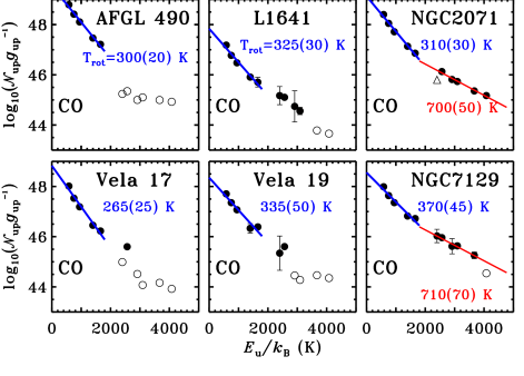
Figure 1: Rotational diagrams of CO. The base-10 logarithm of the number of emitting molecules from the upper level, $\mathcal{N}_{\mathrm{up}}$, divided by the degeneracy of the level, $g_{\mathrm{up}}$, is shown as a function of energy of the upper level in kelvins, $E_{\mathrm{up}}$. Detections are shown as filled circles, whereas three-sigma upper limits are shown as empty circles. Empty upper triangle corresponds to the line flux calculated using a smaller area on the map than the rest of the lines. Blue lines show linear fits to the data and the corresponding rotational temperatures. Errors associated with the least-square linear fit are shown in brackets.

Figure 2: Similar to Figure 1 but for H₂O.

Intermediate-mass YSOs (with $L_{\mathrm{bol}}\sim 10^{2}-10^{3}$ $L_{\odot}$) provide a natural link between low- and high mass protostars, but their far-IR CO and H₂O emission has only been studied for a single protostar position of NGC 7129 FIRS 2 (Fich et al., 2010) and the outflow position of NGC 2071 (Neufeld et al., 2014). CO emission alone was analyzed for two intermediate-mass protostars in Orion, HOPS 288 and 370 (Manoj et al., 2013). In this paper, we present the analysis of PACS spectra for the full sample of intermediate-mass protostars from the ‘Water in star forming regions with Herschel’ (WISH) key program (van Dishoeck et al., 2011), including the maps of NGC 7129 and NGC 2071 centered on the YSO position. These results complement the work by Wampfler et al. (2013), which describes the OH excitation in our source sample and the sample of low- and high-mass protostars for which CO and H₂O emission is discussed in Karska et al. (2013, 2014a). The main question addressed is whether CO and H₂O rotational temperatures differ from low- to high-mass protostars.

The paper is organized as follows. §2 briefly introduces the observations, §3 the excitation analysis using rotational diagrams, and §4 discusses the results.

2 Observations

Table 1: CO and H₂O rotational excitation

Source	$D$	$L_{\mathrm{bol}}$	Warm CO		Hot CO		H2O
	(pc)	($L_{\odot}$)	$T_{\mathrm{rot}}$(K)	$\mathrm{log}_{\mathrm{10}}\mathcal{N}$	$T_{\mathrm{rot}}$(K)	$\mathrm{log}_{\mathrm{10}}\mathcal{N}$	$T_{\mathrm{rot}}$(K)	$\mathrm{log}_{\mathrm{10}}\mathcal{N}$
AFGL 490	1000	2000	300(20)	51.6(0.1)	…	…	90(100)	48.3(1.2)
L 1641 S3 MMS1	465	70	325(30)	49.9(0.1)	…	…	150(100)	46.8(0.1)
NGC 2071	422	520	310(30)	51.2(0.1)	700(50)	50.1(0.1)	135(100)	47.9(0.1)
Vela 17	700	715	265(25)	50.8(0.2)	…	…	90(40)	47.8(0.5)
Vela 19	700	776	335(50)	50.4(0.2)	…	…	130(80)	47.2(0.4)
NGC 7129 FIRS 2	1250	430	370(45)	50.7(0.2)	710(70)	49.9(0.2)	130(50)	47.8(0.1)

Our sample includes 6 YSOs with bolometric luminosities from 70 to 2000 $L_{\odot}$ and located at an average distance of 700 pc (see Table 1). The sources were selected based on their small distances ($\lesssim$ 1 kpc) and location accessible for follow-up observations from the southern hemisphere (for more details see §4.4.2. in van Dishoeck et al., 2011). Spectroscopy for all sources was obtained with PACS as part of the WISH program. For observing details see Table 2 in the Appendix.

With PACS, we obtained single footprint spectral maps covering a field of view of $\sim 47^{\prime\prime}\times 47^{\prime\prime}$ and resolved into 5$\times$5 array of spatial pixels (spaxels) of $\sim 9.4^{\prime\prime}\times 9.4^{\prime\prime}$ each. At the distance to the sources, the full array corresponds to spatial scales of $\sim 2-6\times 10^{4}$ AU in diameter, of the order of full maps of low-mass YSOs ($\sim 10^{4}$ AU) in Karska et al. (2013) and the central spaxel spectra of more distant high-mass YSOs ($\sim 3\times 10^{4}$ AU) in Karska et al. (2014a).

The observations were taken in the line spectroscopy mode, which provide deep integrations of 0.5–2 $\mu$m wide spectral regions within the $\sim$55–210 $\mu$m PACS range. Two nod positions were used for chopping 3^′ on each side of the source (for details of our observing strategy and basic reduction methods, see Karska et al., 2013). The full list of targeted CO and H₂O lines and the calculated line fluxes are shown in Table 3 in the Appendix. The quality of the spectra is illustrated in Figure 4 in the Appendix. We note that the simultaneous non-detections of the H₂O 7₁₆-7₀₇ line at 84.7 $\mu$m and detections of the H₂O 8₁₈-7₀₇ line at 63.3 $\mu$m in L 1641, NGC 2071, and NGC 7129 FIRS 2 are related to the structure of the H₂O energy levels and not the differences in the sensitivities of the instrument in the 2nd and 3rd order observations. The 8₁₈-7₀₇ line is a backbone transition, with the Einstein A coefficient higher than the one for the 7₁₆-7₀₇ line.

The data reduction was done using HIPE v.13 with Calibration Tree 65 and subsequent analysis with customized IDL programs (see e.g. Karska et al., 2014b). The fluxes were calculated using the emission from the entire maps. Figure 5 in the Appendix illustrates that both the line and continuum emission peaks approximately at the source position, with small shifts in continuum due to mispointing. The extent of the line emission follows typically the continuum pattern with the exception of Vela 17 where the line emission extends from NE to SW direction, while the continuum is centrally peaked. There is no contamination detected from the nearby sources or their outflows in the targeted regions.

3 Rotational diagrams

3.1 Results

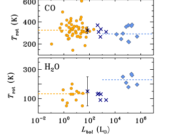
Figure 3: Rotational temperatures of ‘warm’ ($E_{\mathrm{up}}=14-24$) CO (top) and H₂O (bottom) as function of bolometric luminosity. Orange circles show YSOs from Green et al. (2013), Karska et al. (2013), and Manoj et al. (2013). Dark blue crosses show intermediate-mass YSOs from the WISH program and light blue diamonds high-mass YSOs from Karska et al. (2014a). A few sources with luminosities $\sim 10^{2}$ $L_{\odot}$ shown in orange crosses are from Manoj et al. (2013) and can be also regarded as intermediate-mass YSOs. Uncertainties of the CO and H₂O rotational temperatures are shown for L1641 S3 MMS1, which is representative of the sample.

Figure 1 shows rotational diagrams of CO calculated for all sources in the same way as in Karska et al. (2014a). The corresponding rotational temperatures, $T_{\mathrm{rot}}$, and total numbers of emitting molecules, $\mathcal{N}$, are shown in Table 1.

All sources show a 300 K, ‘warm’ CO component (Manoj et al., 2013; Karska et al., 2013; Green et al., 2013), with a mean temperature of $\sim 320$ K for the range of total numbers of emitting molecules, $\mathcal{N}\sim 10^{50}-10^{51}$. In addition, NGC2071 and NGC7129 show a ‘hot’ CO component with temperatures of $\sim 700$ K and $\mathcal{N}\sim 10^{50}$.

The rotational diagrams for H₂O, presented in Figure 2, show a single component with a mean temperature of $\sim 120$ K. The scatter due to subthermal excitation and high opacities exceeds the uncertainties in the observed fluxes, similar to diagrams of low- and high-mass YSOs (for the discussion of both effects see §4.2.2 of Karska et al., 2014a). The corresponding numbers of emitting molecules are about 3 orders of magnitude lower than for CO, $\mathcal{N}\sim 10^{47}-10^{48}$.

3.2 Comparison to low- and high-mass sources

Figure 3 shows a comparison between rotational temperatures obtained for CO and H₂O for the intermediate-mass sources presented here and these quantities determined in the same way for low- and high-mass YSOs. The comparison is restricted only to the ‘warm’ component seen in CO rotational diagrams due to the low number of sources with detections of the ‘hot’ CO component; those will be discussed in detail in Karska et al. (in prep.). A bolometric luminosity is used here as a proxy for the protostellar mass, but in fact some of our intermediate-mass sources may be a collection of unresolved low-mass protostars.

The median $T_{\mathrm{rot}}$ of CO in low-mass protostars is 325 K, using the results from the WISH (Karska et al., 2013), ‘Dust, Ice, and Gas in Time’ (Green et al., 2013), and ‘Herschel Orion Protostar Survey’ (Manoj et al., 2013) programs for a total of about 50 sources. A comparable value of $\sim$290 K was found for 10 high-mass sources ($L_{\mathrm{bol}}\sim 10^{4}-10^{6}$ $L_{\odot}$) in Karska et al. (2014a). The range of CO $T_{\mathrm{rot}}$ of 265-370 K (see Table 1) determined here for intermediate-mass YSOs is thus fully consistent with previous results. The fact that the 300 K CO component does not depend on the source bolometric luminosity over 6 orders of magnitude suggests the origin in a shock associated with the jet / winds impact on the envelope rather than in a photodissociation region where $T_{\mathrm{rot}}$ should scale with the UV flux and luminosity (van Kempen et al., 2010; Visser et al., 2012; Manoj et al., 2013; Flower & Pineau des Forêts, 2013; Kristensen et al., 2013).

The median H₂O rotational temperatures (see the bottom panel of Figure 3) for low- and high-mass YSOs are $\sim 130$ K and $\sim 230$ K, respectively (Karska et al., 2013, 2014a). The range of temperatures obtained for the intermediate-mass YSOs (90-150 K, Table 1) is thus comparable to the low-mass sources. However, the uncertainties in the rotational temperatures are high, of the order of $\sim 100$ K, and do not account for the optical depth effects, the density effects, and the possible complexity of the line profiles (absorption and emission components). It is therefore unclear if there is a true jump in rotational temperatures at $L_{\mathrm{bol}}\sim 10^{4}$ $L_{\odot}$, or a smooth trend toward higher values of $T_{\mathrm{rot}}$. In either case, these higher excitation temperatures could be due to higher densities in the more massive envelopes.

4 Summary

We analyze the excitation of far-infrared CO and H₂O lines in 6 intermediate-mass YSOs observed in the WISH survey and compare the results to low- and high-mass protostars. Rotational temperatures of CO and H₂O are found to be $\sim 320$ K and $\sim 120$ K, respectively, and are consistent with low-mass and high-mass YSOs within the uncertainties. The large uncertainties in the H₂O rotational temperatures, of the order of 100 K, and the order of magnitude gap in the bolometric luminosity between intermediate- and high-mass protostars does not allow us to conclude whether the changes are a smooth function of luminosity. Still, the similarities in rotational temperatures seen for sources with luminosities spanning 6 orders of magnitude and probed at different spatial scales strongly suggest the same excitation mechanism, the UV-irradiated shocks associated with jets and winds for all sources across the luminosity range (Kristensen et al., 2013; Karska et al., 2014b; Mottram et al., 2014).

Appendix A Supplementary material

Table 2 shows the observing log of PACS observations including observations identifications (OBSID), observation day (OD), date of observation, total integration time, and pointed coordinates (RA, DEC). Table 3 shows molecular data and observed lines fluxes and upper limits for all sources that are analyzed in the paper. Figure 4 shows selected spectral regions to illustrate the quality of the data. Figure 5 illustrates the patterns of continuum emission at 145 $\mu$m and the CO 18-17 line emission at 144 $\mu$m toward all the sources.

Table 2: Log of PACS observations

Source	OBSID	OD	Date	Total time	RA	DEC
				(s)	(h m s)	(o ′ ′′)
AFGL 490	1342202582	454	2010-08-11	3882	3 27 38.40	+58 47 08.0
	1342191353	290	2010-02-28	2029	3 27 38.40	+58 47 08.0
L1641 S3 MMS1	1342226194	823	2011-08-14	3882	5 39 55.900	-7 30 28.00
	1342226195	823	2011-08-14	1987	5 39 55.900	-7 30 28.00
NGC 2071	1342218760	703	2011-04-17	3882	5 47 04.40	+0 21 49.00
	1342218761	703	2011-04-17	1987	5 47 04.40	+0 21 49.00
Vela IRS 17	1342209407	551	2010-11-16	3882	8 46 34.70	-43 54 30.5
	1342211844	594	2010-12-28	1987	8 46 34.70	-43 54 30.5
Vela IRS 19	1342210189	552	2010-11-16	3882	8 48 48.50	-43 32 29.0
	1342210190	552	2010-11-16	1987	8 48 48.50	-43 32 29.0
NGC 7129 FIRS2	1342186321	165	2009-10-26	3895	21 43 01.70	+66 03 23.6
	1342186322	165	2009-10-26	2000	21 43 01.70	+66 03 23.6

Table 3: Molecular data and observed line fluxes

Species	Transition	Wave.	Rest Freq.	$E_{\mathrm{u}}$/$k_{\mathrm{B}}$	$A_{\mathrm{ul}}$	AFGL 490	L 1641	NGC 2071	Vela 17	Vela 19	NGC 7129 FIRS 2
		($\mu$m)	(GHz)	(K)	(s-1)	Fluxes (10-20 W cm-2)
CO	14-13	185.999	1611.8	580.5	2.7(-4)	$11.01\pm 0.11$	$5.00\pm 0.10$	$100.13\pm 0.69$	$14.92\pm 0.15$	$7.38\pm 0.10$	$4.41\pm 0.07$
H2O	221-212	180.488	1661.0	194.1	3.1(-2)	$1.62\pm 0.07$	$0.69\pm 0.06$	$12.95\pm 0.09$	$2.74\pm 0.06$	$0.74\pm 0.12$	$1.28\pm 0.05$
H2O	212-101	179.527	1669.9	114.4	5.6(-2)	absorption	$1.69\pm 0.06$	$39.81\pm 0.40$	$9.65\pm 0.08$	$2.88\pm 0.06$	$3.85\pm 0.08$
H2O	303-212	174.626	1716.8	196.8	5.1(-2)	$4.36\pm 0.08$	$2.25\pm 0.06$	$36.97\pm 0.30$	$6.58\pm 0.07$	$3.01\pm 0.11$	$3.13\pm 0.07$
CO	16-15	162.812	1841.3	751.7	4.1(-4)	$8.84\pm 0.11$	$3.76\pm 0.09$	$85.61\pm 0.45$	$9.48\pm 0.18$	$6.32\pm 0.08$	$3.77\pm 0.07$
CO	18-17	144.784	2070.6	945.0	5.7(-4)	$7.74\pm 0.12$	$3.36\pm 0.13$	$70.00\pm 0.65$	$7.62\pm 0.18$	$5.84\pm 0.08$	$3.51\pm 0.13$
H2O	313-202	138.528	2164.1	204.7	1.3(-1)	$2.86\pm 0.08$	$1.57\pm 0.07$	$25.60\pm 0.14$	$3.99\pm 0.06$	$1.81\pm 0.06$	$2.23\pm 0.06$
H2O	404-313	125.354	2391.6	319.5	1.7(-1)	$0.89\pm 0.11$	$1.80\pm 0.05$	$15.52\pm 0.20$	$2.19\pm 0.10$	$1.48\pm 0.11$	$1.57\pm 0.08$
CO	22-21	118.581	2528.2	1397.4	1.0(-3)	$4.61\pm 0.15$	$2.37\pm 0.11$	$49.00\pm 0.26$	$3.68\pm 0.15$	$2.78\pm 0.52$	$2.70\pm 0.11$
CO	24-23	108.763	2756.4	1656.5	1.3(-3)	$3.91\pm 0.34$	$2.25\pm 0.43$	$38.80\pm 0.96$	$3.30\pm 0.29$	$4.80\pm 0.46$	$3.23\pm 0.33$
H2O	221-110	108.073	2774.0	194.1	2.6(-1)	$1.47\pm 0.17$	$3.19\pm 0.14$	$35.30\pm 0.30$	$5.83\pm 0.16$	$3.12\pm 0.16$	$4.51\pm 0.12$
CO	29-28	90.163	3325.0	2399.8	2.1(-3)	$<0.1$	$1.58\pm 0.57$	$>8.17$	$<0.46$	$1.04\pm 0.71$	$1.58\pm 0.42$
H2O	322-211	89.988	3331.5	296.8	3.5(-1)	$<0.1$	$0.99\pm 0.57$	$10.21\pm 0.30$	$<0.46$	$<0.20$	$1.25\pm 0.42$
CO	30-29	87.190	3438.4	2564.9	2.3(-3)	$<0.15$	$1.58\pm 0.09$	$20.37\pm 0.13$	$2.19\pm 0.19$	$2.22\pm 0.16$	$1.58\pm 0.07$
H2O	716-707	84.767	3536.7	1013.2	2.1(-1)	$<0.1$	$<0.10$	$<1.09$	$<0.13$	$<0.16$	$<0.10$
CO	32-31	81.806	3664.7	2911.2	2.7(-3)	$<0.1$	$0.92\pm 0.57$	$13.16\pm 0.40$	$<0.24$	$<0.21$	$0.96\pm 0.29$
CO	33-32	79.360	3777.6	3092.5	3.0(-3)	$<0.13$	$0.48\pm 0.07$	$12.56\pm 0.24$	$<0.10$	$<0.16$	$1.14\pm 0.09$
H2O	615-524	78.928	3798.3	781.1	4.6(-1)	$<0.17$	$0.53\pm 0.09$	$2.71\pm 0.43$	$<0.16$	$<0.23$	$<0.16$
CO	36-35	72.843	4115.6	3668.8	3.6(-3)	$<0.15$	$<0.04$	$7.74\pm 0.21$	$<0.18$	$<0.36$	$0.70\pm 0.09$
CO	38-37	69.074	4340.1	4080.0	4.1(-3)	$<0.16$	$<0.11$	$6.36\pm 0.35$	$<0.13$	$<0.35$	$<0.17$
H2O	818-707	63.324	4734.3	1070.7	1.8(0)	$<0.27$	$0.64\pm 0.11$	$8.36\pm 0.37$	$<0.15$	$<0.23$	$0.57\pm 0.07$

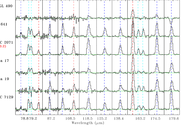
Figure 4: Spectral scans covering selected H₂O, CO and OH lines in the intermediate mass protostars from the WISH program. The rest wavelength of each line is indicated by dashed lines: blue for H₂O, red for CO, and light blue for OH.

Figure 5: PACS spectral maps in the CO 18-17 line at 144 $\mu$m and the continuum emission at 145 $\mu$m in orange contours corresponding to 30%, 50%, 70%, and 90% of the peak value written in the bottom left corner of each map. Wavelengths in microns are translated to the velocity scale on the X-axis using laboratory wavelengths (see Table 3) of the species and cover the range from -600 to 600 km s^-1. The Y-axis shows fluxes in Jy normalized to the spaxel with the brightest line on the map in a range -0.2 to 1.2.