Anisotropic magnetoresistance driven by surface spin orbit scattering

Abstract

In a bilayer consisting of an insulator (I) and a ferromagnetic metal (FM), interfacial spin orbit scattering leads to spin mixing of the two conducting channels of the FM, which results in an unconventional anisotropic magnetoresistance (AMR). We theoretically investigate the magnetotransport in such bilayer structures by solving the spinor Boltzmann transport equation with generalized Fuchs-Sondheimer boundary condition that takes into account the effect of spin orbit scattering at the interface. We find that the new AMR exhibits a peculiar angular dependence which can serve as a genuine experimental signature. We also determine the dependence of the AMR on film thickness as well as spin polarization of the FM.

Anisotropic magnetoresistance (AMR) is a generic magnetotransport property of ferromagnetic metals. In general, the longitudinal resistance of a bulk polycrystalline ferromagnetic metal only depends on the relative orientations of the magnetization vector and the current, which can be cast in the form McGuire and Potter (1975),

$$\rho=\rho_{0}+\Delta\rho_{b}(\hat{\mathbf{j}}_{e}\cdot\mathbf{m})^{2}\,$$ (1)

where $\hat{\mathbf{j}}_{e}=\mathbf{j}_{e}/j_{e}$ is the unit vector in the direction of the current density, $\mathbf{m}$ is the unit vector in the direction of the magnetization, $\rho_{0}$ is the isotropic longitudinal resistivity and $\Delta\rho_{b}$ quantifies the magnitude of the bulk AMR effect (typically $\Delta\rho_{b}\sim 1\%\,$for transition metals and their alloys). The effect has found many practical applications in magnetic recording and sensor devices Haji-Sheikh (2008).

Recently, the AMR effect has also played a key role in measurements of spin Hall angle Mosendz et al. (2010); Feng et al. (2012); Mosendz et al. (2010) as well as spin torque generation Liu et al. (2012, 2012, 2011); Mellnik et al. (2014) in FM/heavy-metal and FM/topological-insulator (TI) bilayers. The structural inversion asymmetry of these structures, combined with strong spin orbit coupling in the non-magnetic layers, generates a large Rashba-type spin-orbit coupling Wang et al. (2013); Tokatly et al. (2015); Haney et al. (2013)

$$\hat{V}_{s.o.}=-\lambda_{c}^{2}V^{\prime}\left(z\right)\bm{\sigma}\cdot\left(\mathbf{\hat{p}}\times\mathbf{z}\right)\,$$ (2)

where $\bm{\sigma}$ is the Pauli spin matrix, $\mathbf{\hat{p}}$ is the momentum operator, $\lambda_{c}$ is the effective Compton wave length, $\mathbf{z}$ is the unit vector normal to the interface, $V(z)$ is the potential in the vicinity of the interface (which only varies in the $z-$ direction), and $V^{\prime}(z)$ is its derivative, which is large only in the interfacial region. A natural question arises: will the interfacial spin orbit interaction alter the AMR in the FM layer? At first glance, one might think the spin orbit interaction, commuting with the total in-plane momentum, $p_{x}$ and $p_{y}$, cannot alter the in-plane resistivity. However, this argument fails in a ferromagnetic metal since the in-plane momenta of either spin component are not separately conserved, and the spin-orbit coupling transfers momentum from one spin channel into the other.

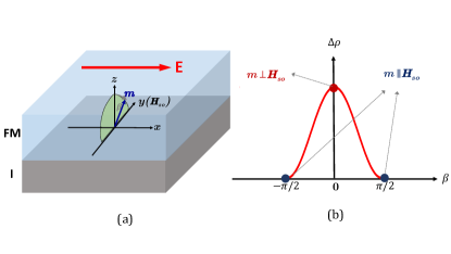
Figure 1: Schematics of the transverse AMR effect induced by surface spin orbit scattering in a FM/I bilayer. The longitudinal resistivity changes when the magnetization $\mathbf{m}$ is rotated in the plane perpendicular to the electric field $\mathbf{E}$. Specifically, the resistivity is at a maximum when $\mathbf{m}$ is perpendicular to the interface (i.e., $\beta=0$) and reaches a minimum when $\mathbf{m}$ lies in the plane of the interface (i.e., $\beta=\pm\pi/2$). This unusual AMR effect arises from spin mixing of the conducting channels of the FM, which depends on the relative directions of the magnetization $\mathbf{m}$ and the effective spin orbital field $\mathbf{H}_{so}\sim\mathbf{z}\times\mathbf{E}$.

In this paper, we show that, in the presence of surface spin orbit scattering, the AMR of a ferromagnet exhibits an angular dependence that is distinctly different from the conventional one described by Eq. (1). As shown in Fig. 1, when the magnetization vector $\mathbf{m}$ is swept in the plane perpendicular to the applied electric field $\mathbf{E}$, a variation in the longitudinal resistivity occurs, which has no analogue in Eq. (1): the resistivity has a maximum when $\mathbf{m}$ is along the $z-$axis (i.e., normal to the film plane) and reaches a minimum when $\mathbf{m}$ is along the $y-$axis (i.e., orthogonal to both $\mathbf{E}$ and $\mathbf{z}$), even though the angle between the magnetization and the current does not change. The physical origin of this unconventional angular dependence lies in the concerted actions of surface spin orbit scattering and spin asymmetry in the conductivity of the FM, which can be understood qualitatively within the two-current model Campbell and Fert (1982); Fert (1969). The surface spin orbit scattering plays a crucial role in mixing the two parallel current channels of majority and minority spins; moreover, the degree of spin mixing depends on the relative orientation of the magnetization and the effective magnetic field $\mathbf{H}_{so}\sim\mathbf{j}_{e}\times\mathbf{z}$ seen by the electron spin. Specifically, spin mixing is strong when $\mathbf{m}$ is perpendicular to $\mathbf{H}_{so}$ while it is weak when $\mathbf{m}$ is aligned with $\mathbf{H}_{so}$. The spin mixing causes, as long as the resistivities of the two current channels are not identical, a redistribution of current by decreasing the resistivity of the channel with higher resistivity and increasing the resistivity of the channel with lower resistivity: this results in an overall increase of the total resistivity Campbell and Fert (1982); Fert (1969). The largest resistivity therefore coincides with the largest degree of spin mixing, which occurs when $\mathbf{m}$ is perpendicular to $\mathbf{H}_{so}$.

In the remainder of this paper we present a quantitative theory of the spin-orbit driven AMR in a FM/I bilayer with strong interfacial spin orbit coupling. At variance with previous studies Nakayama et al. (2013); Chen et al. (2013); Zhang and Zhang (2014); Grigoryan et al. (2014); Miao et al. (2014) we exclude from our consideration heavy metals with strong spin-orbit coupling: in fact, we assume that the spin-orbit coupling is negligible in the bulk of the ferromagnet, so as to avoid contamination from the conventional bulk AMR effect.

Our theoretical analysis is based on the spinor form of the semiclassical Boltzmann equation: the non-equilibrium distribution function, $\hat{f}(\mathbf{k,}z)$, is a $2\times 2$ matrix in spin space Zhang et al. (2004); Sheng et al. (1997). For simplicity, we assume same Fermi wave vector $k_{F}$ but different relaxation times for majority and minority electrons, just as in the seminal paper by Valet and Fert in calculating the CPP-GMR Valet and Fert (1993). Such simplification is justified since the essence of our effect is in the difference of the relaxation times (and hence the resistivities) of majority and minority spins, while the exchange splitting is responsible for spin dephasing of the transverse spin component Stiles and Zangwill (2002); Zhang et al. (2004).

The equation of motion for $\hat{f}(\mathbf{k,}z)$ in the steady state is

$$v_{z}\frac{\partial\hat{f}(\mathbf{k,}z)}{\partial z}-eEv_{x}\left(\frac{\partial f_{0}(k)}{\partial\varepsilon_{k}}\right)\hat{I}=-\frac{1}{2}\left\{\hat{\tau}^{-1},\delta\hat{f}(\mathbf{k,}z)\right\}$$ (3)

where $f_{0}(k)$ is the equilibrium distribution function, $\hat{\tau}^{-1}=\left(\tau^{\prime}\right)^{-1}\left(\hat{I}-p\bm{\sigma}\cdot\mathbf{m}\right)$ is the spin dependent relaxation rate with $\left(\tau^{\prime}\right)^{-1}=\left[\left(\tau_{\uparrow}\right)^{-1}+\left(\tau_{\downarrow}\right)^{-1}\right]/2$ and $p\equiv\left[\left(\tau_{\downarrow}\right)^{-1}-\left(\tau_{\uparrow}\right)^{-1}\right]/\left[\left(\tau_{\uparrow}\right)^{-1}+\left(\tau_{\downarrow}\right)^{-1}\right]$ being, respectively, the average momentum relaxation rate and the spin asymmetry in resistivity, $\tau_{\uparrow}$ and $\tau_{\downarrow}$ being the momentum lifetimes of the two spin channels, and $\left\{\text{ },\right\}$ standing for an anticommutator. Notice that in the collision term of Eq. (3) we require that the difference

$$\delta\hat{f}(\mathbf{k},z)\equiv\hat{f}(\mathbf{k},z)-\hat{f}_{l.e.}(k,z)$$ (4)

between the non-equilibrium distribution and a local equilibrium distribution Haug and Jauho (2007); Giuliani and Vignale (2008); W. H. Bulter (2001)

$$\hat{f}_{l.e.}(k,z)=f_{0}(k)\hat{I}+\frac{\partial f_{0}}{\partial\varepsilon_{k}}\left[\mu_{0}\left(z\right)\hat{I}+\bm{\sigma}\cdot\bm{\mu}_{s}\left(z\right)\right]$$ (5)

tend to zero for long times. The parameters $\mu_{0}(z)$ and $\bm{\mu}_{s}(z)$ of the local distribution are fixed in such a way that the condition

$$\int d^{3}\mathbf{k}\left[\hat{f}(\mathbf{k,}z)-\hat{f}_{l.e.}(k,z)\right]=0$$ (6)

is self-consistently satisfied. By doing this, we satisfy the physical requirements of particle and spin conservation in the collision processes, as well as the continuity equations that go with them.

To solve the Boltzmann equation, we further separate the distribution function into an equilibrium part and a small non-equilibrium perturbation, i.e.,

$$\hat{f}(\mathbf{k,}z)=f_{0}(k)\hat{I}\mathbf{+}\frac{\partial f_{0}}{\partial\varepsilon_{k}}\left[g\left(\mathbf{k,}z\right)\hat{I}+\mathbf{h}(\mathbf{k,}z)\cdot\bm{\sigma}\right]$$ (7)

where $g\left(\mathbf{k,}z\right)\hat{I}$ and $\mathbf{h}(\mathbf{k,}z)\cdot\bm{\sigma}$ are the spin-independent and spin-dependent components of the non-equilibrium distribution. By inserting Eq. (7) into Eq. (3), we obtain a set of coupled equations for the scalar and vector parts of the distribution function

$$v_{z}\frac{\partial g}{\partial z}-eE_{x}v_{x}=-\frac{g\mathbf{-}\mu_{0}-p\left(h_{\parallel}-\mu_{s\parallel}\right)}{\tau^{\prime}}$$ (8)

$$v_{z}\frac{\partial h_{\parallel}}{\partial z}=-\frac{h_{\parallel}-\mu_{s\parallel}-p\left(g-\mu_{0}\right)}{\tau^{\prime}}$$ (9)

and

$$v_{z}\frac{\partial\mathbf{h}_{\perp}}{\partial z}=-\frac{\mathbf{h}_{\perp}-\bm{\mu}_{s\perp}}{\tau^{\prime}}$$ (10)

where $h_{\parallel}=\mathbf{m\cdot h}(\mathbf{k,}z)$, $\mu_{s\parallel}=\mathbf{m\cdot}\bm{\mu}_{s}\left(z\right)$, $\mathbf{h}_{\perp}=\left(\mathbf{m\times h}\right)\mathbf{\times m}$ and $\bm{\mu}_{s\perp}=\left(\mathbf{m\times}\bm{\mu}_{s}\right)\mathbf{\times m}$. The equations (8)-(10) have the general solutions

$$g^{\pm}\left(\mathbf{k,}z\right)=e\tau v_{x}E_{x}+A_{\mathbf{k}}^{\pm}e^{\mp\frac{\left(1-p\right)z}{\left|v_{z}\right|\tau^{\prime}}}+B_{\mathbf{k}}^{\pm}e^{\mp\frac{\left(1+p\right)z}{\left|v_{z}\right|\tau^{\prime}}}+\sum_{\alpha}\int_{0}^{z}dt\left[\mu_{0}\left(t\right)+\alpha\mu_{s\parallel}\left(t\right)\right]\frac{\partial}{\partial t}e^{\mp\frac{\left(1-\alpha p\right)\left(z-t\right)}{\left|v_{z}\right|\tau^{\prime}}}\,,$$ (11)

$$h_{\parallel}^{\pm}\left(\mathbf{k,}z\right)=pe\tau v_{x}E_{x}+A_{\mathbf{k}}^{\pm}e^{\mp\frac{\left(1-p\right)z}{\left|v_{z}\right|\tau^{\prime}}}-B_{\mathbf{k}}^{\pm}e^{\mp\frac{\left(1+p\right)z}{\left|v_{z}\right|\tau^{\prime}}}+\sum_{\alpha}\alpha\int_{0}^{z}dt\left[\mu_{0}\left(t\right)+\alpha\mu_{s\parallel}\left(t\right)\right]\frac{\partial}{\partial t}e^{\mp\frac{\left(1-\alpha p\right)\left(z-t\right)}{\left|v_{z}\right|\tau^{\prime}}}\,,$$ (12)

and

$$\mathbf{h}_{\perp}^{\pm}\left(\mathbf{k,}z\right)\mathbf{=C_{\mathbf{k}}^{\pm}}e^{\mp\frac{z}{\left|v_{z}\right|\tau^{\prime}}}+\int_{0}^{z}dt\bm{\mu}_{s\perp}\left(t\right)\frac{\partial}{\partial t}e^{\mp\frac{\left(z-t\right)}{\left|v_{z}\right|\tau^{\prime}}}\,,$$ (13)

where the superscript $+$ labels the solution for $v_{z}>0$ and the subscript $-$ for $v_{z}<0$. The sum over $\alpha$ runs over the values $\alpha=\pm 1$. The four unknown constants $A_{\mathbf{k}}$, $B_{\mathbf{k}}$, and $\mathbf{C_{\mathbf{k}}}$ (where $\mathbf{C_{\mathbf{k}}}$ is a vector orthogonal to $\mathbf{m}$, hence with only two components) will now be determined from the boundary conditions.

Up to this point, the interfacial spin-orbit interaction has not appeared in our calculations. In particular, the collision term in Eq. (3) did not contain it, and therefore conserved spin. The spin-orbit coupling appears in the boundary condition that connects the distribution function for electrons impinging on the interface (label $-$) to the distribution function for electrons that are scattered off the interface (label $+$). Specifically, in order to take into account the rotation of spin upon scattering off the interface with the potential

$$\hat{V}_{scat.}=V_{b}\Theta\left(-z\right)-\left(V_{b}\lambda_{c}^{2}\right)\delta\left(z\right)\bm{\sigma}\cdot\left(\mathbf{\hat{p}}\times\mathbf{z}\right)$$ (14)

(where $V_{b}$ is the barrier height of the insulator, $\Theta\left(z\right)$ is the unit step function, $\mathbf{z}$ is the unit vector normal to the interface and the delta function confines the SO coupling to the interface at $z=0$), we introduce the following spinor generalization of the Fuchs-Sondheimer boundary condition Fuchs (1938); Sondheimer (1950); Reuter and Sondheimer (1948):

$$\hat{f}^{+}(\mathbf{k};z=0)=s_{I}\hat{R}^{{\dagger}}\hat{f}^{-}(\mathbf{k;}z=0)\hat{R}+\left(1-s_{I}\right)f_{0}\hat{I}$$ (15)

where the superscripts $+$ and $-$ correspond to the distribution functions with $v_{z}>0$ and $v_{x}<0$ respectively, the parameter $s_{I}$ varies between 0 and 1, characterizing the fraction of electrons being specularly reflected Reuter and Sondheimer (1948) ($s_{I}=1$ when the interface is perfectly smooth and $s_{I}=0$ when the interface is extremely rough) and $\hat{R}$ is a $2\times 2$ reflection amplitude matrix in spin space which captures the spin rotation of the reflected electrons. Explicitly,

$$\hat{R}=\frac{\left[-k_{b}^{2}+\left(\lambda_{c}k_{b}\right)^{4}q^{2}\right]\hat{I}+2i\left(\lambda_{c}k_{b}\right)^{2}k_{z}\bm{\sigma}\cdot\left(\mathbf{q}\times\mathbf{z}\right)}{\left(\kappa-ik_{z}\right)^{2}-\left(\lambda_{c}k_{b}\right)^{4}q^{2}}$$ (16)

where $\kappa\equiv\sqrt{k_{b}^{2}-k_{z}^{2}}$ with $k_{b}\equiv\sqrt{2m_{e}^{\ast}V_{b}/\hbar^{2}}$. The derivation of $\hat{R}$ is presented in the appendix. It must be pointed out that the boundary condition described by Eq. (15) neglects the interference between incident and reflected states. However, we neglect this quantum coherence by assuming a rough interface. This is justified when the characteristic size as well as the correlation length of the surface roughness is comparable to the Fermi wavelength in which case the phase coherence is destroyed by surface roughness Ziman (1960).

For simplicity, we assume spin independent specular reflection only at the outer surface of the FM layer ($z=d$), i.e.,

$$\hat{f}^{+}(\mathbf{k;}z=d)=\hat{f}^{-}(\mathbf{k;}z=d)$$ (17)

Neglecting spin-dependent scattering from the other surface simplifies the calculation without altering any qualitative features of the results. By inserting Eq. (7) into the boundary conditions as well as Eq. (6) , we can find unique solutions for $\hat{f}(\mathbf{k,}z)$ and the charge current density can be calculated as

$$\mathbf{j}_{e}\left(z\right)=\frac{-e}{\left(2\pi\right)^{3}}Tr\int d\mathbf{k}\hat{f}(\mathbf{k,}z)\mathbf{v}$$ (18)

After some algebra, we find the charge current density up to second order in the spin orbit coupling, i.e., $O\left(\left(\lambda_{c}k_{b}\right)^{4}\right)$

$$\mathbf{j}_{e}\left(z\right)=c_{0}E_{x}\left\{\left[1\mathbf{-}\alpha_{xx}^{(1)}\left(z\right)-\alpha_{xx}^{(2)}\left(z\right)\right]\mathbf{\hat{x}+}\alpha_{yx}\left(z\right)\mathbf{\hat{y}}\right\}$$ (19)

where $c_{0}=e^{2}\tau k_{F}^{3}/3\pi m_{e}^{\ast}$ is Drude conductivity and two position dependent coefficients read

$$\alpha_{xx}^{(1)}\left(z\right)=\left(1-s_{I}\right)\sum_{\sigma}\left(1+\sigma p\right)F_{p\sigma}\left(z\right)$$ (20)

$$\alpha_{xx}^{(2)}\left(z\right)=s_{I}p\left(\lambda_{c}k_{F}\right)^{4}\left[4-\left(m_{x}^{2}+3m_{y}^{2}\right)\right]\sum_{\sigma}\sigma G_{p\sigma}\left(z\right)\,,$$ (21)

and

$$\alpha_{yx}\left(z\right)=s_{I}p\left(\lambda_{c}k_{F}\right)^{4}m_{x}m_{y}\sum_{\sigma}\sigma G_{p\sigma}\left(z\right)\,,$$ (22)

where

$$F_{p\sigma}\left(z\right)\equiv\frac{3}{4}\int_{0}^{1}d\xi\frac{(1-\xi^{2})\cosh\left[\frac{\left(1-\sigma p\right)\left(d-z\right)}{\xi\lambda_{0}\left(1-p^{2}\right)}\right]}{\exp\left[\frac{\left(1-\sigma p\right)d}{\xi\lambda_{0}\left(1-p^{2}\right)}\right]-s_{I}\exp\left[-\frac{\left(1-\sigma p\right)d}{\xi\lambda_{0}\left(1-p^{2}\right)}\right]}$$ (23)

and

$$G_{p\sigma}\left(z\right)\equiv\frac{3}{2}\int_{0}^{1}d\xi\frac{\xi(1-\xi^{2})^{3/2}\cosh\left[\frac{\left(1-\sigma p\right)\left(d-z\right)}{\xi\lambda_{0}\left(1-p^{2}\right)}\right]}{\exp\left[\frac{\left(1-\sigma p\right)d}{\xi\lambda_{0}\left(1-p^{2}\right)}\right]-s_{I}\exp\left[-\frac{\left(1-\sigma p\right)d}{\xi\lambda_{0}\left(1-p^{2}\right)}\right]}\,,$$ (24)

and $\lambda_{0}\equiv v_{F}(\tau_{\uparrow}+\tau_{\downarrow})/2$ is the average electron mean free path. The first term, $\alpha_{xx}^{(1)}$, is independent of the magnetization direction: it is the resistivity due to interfacial roughness Ziman (1960). The third term, $\alpha_{yx}$, corresponds to the well-known planar Hall effect McGuire and Potter (1975); Campbell and Fert (1982).

The second term, $\alpha_{xx}^{(2)}$, describes the new AMR effect. We note that this effect is of second order in the spin-orbit coupling and vanishes when the spin polarization $p=0$. The experimentally relevant quantity is the spatially averaged longitudinal resistivity, which is obtained from the formula $\rho_{xx}^{-1}\left(d\right)=\left(1/d\right)\int_{0}^{d}dz~{}j_{e,x}\left(z\right)/E_{x}$. As we discussed earlier, the bulk spin-orbit coupling (not included in our calculation) produces a conventional AMR with angular dependence shown in Eq. (1). Therefore in general, the longitudinal resistivity of the FM thin film should take the form

$$\rho_{xx}\left(d\right)=\rho_{0}+\Delta\rho_{so}^{\left(b+s\right)}m_{x}^{2}-\Delta\rho_{so}^{\left(s\right)}m_{y}^{2}$$ (25)

where the first term on the rhs of Eq. (25) is the isotropic resistivity and the second term is the AMR with conventional angular dependence of $(\hat{\mathbf{j}}_{e}\cdot\mathbf{m})^{2}$ to which both bulk and surface spin orbit coupling may contribute. The most interesting term is the third term which is solely due to the surface spin orbit scattering and can be distinguished from the bulk AMR based on the different angular dependence.

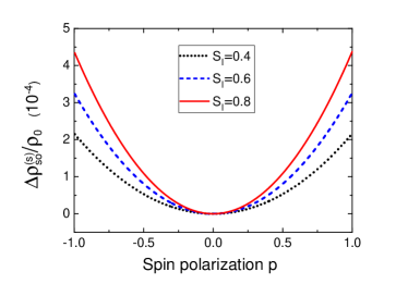
Figure 2: The transverse AMR $\Delta\rho_{so}^{\left(s\right)}$ as a function of the spin polarization $p$ for several different $s_{I}$. Parameters: $\lambda_{c}k_{F}=0.05$, $d/\lambda_{0}=1$.

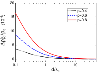
Figure 3: The transverse AMR $\Delta\rho_{so}^{\left(s\right)}$ as a function of $d/\lambda_{0}$ for several different $p$. Parameters: $\lambda_{c}k_{F}=0.05$ and $s_{I}=0.8$.

In Fig. 2, we show $\Delta\rho_{so}^{\left(s\right)}$ (normalized by $\rho_{0}$) as a function of the spin polarization $p$. This figure delivers two main messages. First, $\Delta\rho_{so}^{\left(s\right)}$ is positive when $p\neq 0$. This confirms the angular dependence of the AMR we sketched in Fig. 1(b). The second message is that $\Delta\rho_{so}^{\left(s\right)}$ is an even function of the spin polarization $p$. This is consistent with our two-current model: the spin mixing resistivity only relies on the absolute value of the difference between the two conduction channels but not on the sign of that difference.

In Fig. 3, we show the thickness dependence of the $\Delta\rho_{so}^{\left(s\right)}$ for several values of spin polarization. When the FM layer thickness is much larger than the mean free path, i.e., $d\gg\lambda_{0}$, $\Delta\rho_{so}^{\left(s\right)}$ exhibits a standard $1/d$ thickness dependence as can be analytically worked out via Eq. (24).

Lastly, let us consider the choice of materials for the observation of our predicted AMR. In order to obtain a sizable transverse AMR, it is essential to have a FM/I bilayer with a large difference between the conductivities of majority and minority spin carriers in the ferromagnetic metal, and a strong spin-orbit interaction at the FM/I interface. A very promising system in this respect is Py grown on top of a TI such as Bi₂Se₃, Bi_1.5Sb_0.5Te_1.7Se_1.3 or Sn-doped Bi₂Te_1.7Se_1.3 Ren et al. (2012); Taskin et al. (2011); Ren et al. (2011). Recently, large spin transfer torque Mellnik et al. (2014) and spin-charge conversion Shiomi et al. (2014) effects were observed in these FM/TI bilayers, indicating the presence of strong spin orbit coupling at the interface. Non-topological-oxide/ferromagnetic interfaces may also provide large spin-orbit interaction, as implied by tunneling AMR studies in Fe/MgO/Fe junctions Gao et al. (2007); Chantis et al. (2007) and by magnetic anisotropy analysis at AlOx/Co interface Gao et al. (2007); Manchon et al. (2008). As a final point, we note that the surface spin orbit scattering mechanism should, in principle, also contribute to the transverse AMR that was previously found in Pt/Co/Pt Kobs et al. (2011) and Py/YIG Lu et al. (2013) layered systems.

This work was supported by NSF Grants DMR-1406568 (S.S.-L.Z and G.V.) and ECCS-1404542 (S.S.-L.Z and S. Z.).

Appendix A Appendix: Spinor form reflection amplitude in the presence of interface Rashba spin orbit coupling

In this appendix, we derive the spinor form reflection amplitude given by Eq. (16) in the main text. First, we write down the following piece-wise scattering wave functions corresponding to the interfacial potential described by Eq. (14) in the main text

$$\psi_{\mathbf{k}}\left(\mathbf{r}_{\parallel}\mathbf{,}z>0\right)=\frac{1}{\sqrt{2}}e^{-ik_{z}z}e^{i\mathbf{q\cdot r}_{\parallel}}\chi+\frac{1}{\sqrt{2}}e^{ik_{z}z}e^{i\mathbf{q\cdot r}_{\parallel}}\hat{R}\chi$$ (A1)

and

$$\psi_{\mathbf{k}}\left(\mathbf{r,}z<0\right)=\frac{1}{\sqrt{2}}e^{\kappa z}e^{i\mathbf{q\cdot r}_{\parallel}}\hat{T}\chi$$ (A2)

where $\mathbf{r}_{\parallel}$ is the in-plane position vector, $\mathbf{q}$ and $k_{z}$ are the in-plane and perpendicular-to-plane wave vectors respectively, $\kappa=\sqrt{k_{b}^{2}-k_{z}^{2}}$with $k_{b}\equiv\sqrt{2m_{e}^{\ast}V_{b}/\hbar^{2}}$, $\hat{R}$ and $\hat{T}$ are the $2\times 2$ reflection and transmission amplitude matrices in spin space, and $\chi$ is an arbitrary spinor.

Now we are ready to determine $\hat{R}$ and $\hat{T}$ matrices by the following quantum mechanical matching conditions

$$\psi_{\mathbf{k}}\left(\mathbf{r}_{\parallel}\mathbf{,}0^{+}\right)=\psi_{\mathbf{k}}\left(\mathbf{r}_{\parallel}\mathbf{,}0^{-}\right)$$ (A3)

and

$$\psi_{\mathbf{k}}^{\prime}\left(\mathbf{r}_{\parallel}\mathbf{,}0^{+}\right)-\psi_{\mathbf{k}}^{\prime}\left(\mathbf{r}_{\parallel}\mathbf{,}0^{-}\right)=\left[\left(k_{b}\lambda_{c}\right)^{2}\bm{\sigma}\cdot\left(\mathbf{\hat{p}}\times\mathbf{z}\right)\right]\psi_{\mathbf{k}}\left(\mathbf{r}_{\parallel}\mathbf{,}0\right)$$ (A4)

By placing the scattering wave functions into the above two equations, we find

$$\left(\hat{I}+\hat{R}\right)\chi=\hat{T}\chi$$ (A5)

and

$$\left(-\kappa\hat{T}-ik_{z}\hat{I}+ik_{z}\hat{R}\right)\chi=\left[\left(k_{b}\lambda_{c}\right)^{2}\bm{\sigma}\cdot\left(\mathbf{q}\times\mathbf{z}\right)\right]\hat{T}\chi$$ (A6)

Combining the two equations, we find an equation for $\hat{R}$ only,

$$\left\{\left[\left(\kappa-ik_{z}\right)\hat{I}+\left(k_{b}\lambda_{c}\right)^{2}\bm{\sigma}\cdot\left(\mathbf{q}\times\mathbf{z}\right)\right]\hat{R}+\left(ik_{z}+\kappa\right)\hat{I}+\left(k_{b}\lambda_{c}\right)^{2}\bm{\sigma}\cdot\left(\mathbf{q}\times\mathbf{z}\right)\right\}\chi=0$$ (A7)

For any $\chi$, the equation is valid if

$$\left[\left(\kappa-ik_{z}\right)\hat{I}+\left(k_{b}\lambda_{c}\right)^{2}\bm{\sigma}\cdot\left(\mathbf{q}\times\mathbf{z}\right)\right]\hat{R}+\left(ik_{z}+\kappa\right)\hat{I}+\left(k_{b}\lambda_{c}\right)^{2}\bm{\sigma}\cdot\left(\mathbf{q}\times\mathbf{z}\right)=0$$ (A8)

From Eq. (A8), we find the reflection amplitude matrix

$$\hat{R}=\frac{\left[-k_{b}^{2}+\left(k_{b}\lambda_{c}\right)^{4}q^{2}\right]\hat{I}+2i\left(k_{b}\lambda_{c}\right)^{2}k_{z}\bm{\sigma}\cdot\left(\mathbf{q}\times\mathbf{z}\right)}{\left(ik_{z}-\kappa\right)^{2}-\left(k_{b}\lambda_{c}\right)^{4}q^{2}}$$ (A9)

. Note that $\hat{R}$ is a unitary matrix as can be easily check via Eq. (A9). This unitarity is required by flux conservation.

References

- McGuire and Potter (1975) T. McGuire and R. Potter, IEEE Trans. Magn., 11, 1018 (1975).
- Haji-Sheikh (2008) M. J. Haji-Sheikh, “Sensors: Advancements in modeling, design issues, fabrication and practical applications,” (Springer Berlin Heidelberg, 2008) Chap. 1, pp. 23–43.
- Mosendz et al. (2010) O. Mosendz, V. Vlaminck, J. E. Pearson, F. Y. Fradin, G. E. W. Bauer, S. D. Bader, and A. Hoffmann, Phys. Rev. B, 82, 214403 (2010a).
- Feng et al. (2012) Z. Feng, J. Hu, L. Sun, B. You, D. Wu, J. Du, W. Zhang, A. Hu, Y. Yang, D. M. Tang, B. S. Zhang, and H. F. Ding, Phys. Rev. B, 85, 214423 (2012).
- Mosendz et al. (2010) O. Mosendz, J. E. Pearson, F. Y. Fradin, G. E. W. Bauer, S. D. Bader, and A. Hoffmann, Phys. Rev. Lett., 104, 046601 (2010b).
- Liu et al. (2012) L. Liu, C.-F. Pai, Y. Li, H. W. Tseng, D. C. Ralph, and R. A. Buhrman, Science, 336, 555 (2012a).
- Liu et al. (2012) L. Liu, O. J. Lee, T. J. Gudmundsen, D. C. Ralph, and R. A. Buhrman, Phys. Rev. Lett., 109, 096602 (2012b).
- Liu et al. (2011) L. Liu, T. Moriyama, D. C. Ralph, and R. A. Buhrman, Phys. Rev. Lett., 106, 036601 (2011).
- Mellnik et al. (2014) A. R. Mellnik, J. S. Lee, A. Richardella, J. L. Grab, P. J. Mintun, M. H. Fischer, A. Vaezi, A. Manchon, E.-A. Kim, N. Samarth, and D. C. Ralph, Nature, 511, 449 (2014).
- Wang et al. (2013) X. Wang, J. Xiao, A. Manchon, and S. Maekawa, Phys. Rev. B, 87, 081407 (2013).
- Tokatly et al. (2015) I. V. Tokatly, E. E. Krasovskii, and G. Vignale, Phys. Rev. B, 91, 035403 (2015).
- Haney et al. (2013) P. M. Haney, H.-W. Lee, K.-J. Lee, A. Manchon, and M. D. Stiles, Phys. Rev. B, 87, 174411 (2013).
- Campbell and Fert (1982) I. A. Campbell and A. Fert, “Ferromagnetic materials,” (North-Holland, Amsterdam, 1982) Chap. 9, p. 747.
- Fert (1969) A. Fert, J. Phys. C: Solid State Phys., 2, 1784 (1969).
- Nakayama et al. (2013) H. Nakayama, M. Althammer, Y.-T. Chen, K. Uchida, Y. Kajiwara, D. Kikuchi, T. Ohtani, S. Geprägs, M. Opel, S. Takahashi, R. Gross, G. E. W. Bauer, S. T. B. Goennenwein, and E. Saitoh, Phys. Rev. Lett., 110, 206601 (2013).
- Chen et al. (2013) Y.-T. Chen, S. Takahashi, H. Nakayama, M. Althammer, S. T. B. Goennenwein, E. Saitoh, and G. E. W. Bauer, Phys. Rev. B, 87, 144411 (2013).
- Zhang and Zhang (2014) S. S.-L. Zhang and S. Zhang, J. Appl. Phys., 115, 17C703 (2014).
- Grigoryan et al. (2014) V. L. Grigoryan, W. Guo, G. E. W. Bauer, and J. Xiao, Phys. Rev. B, 90, 161412 (2014).
- Miao et al. (2014) B. F. Miao, S. Y. Huang, D. Qu, and C. L. Chien, Phys. Rev. Lett., 112, 236601 (2014).
- Zhang et al. (2004) J. Zhang, P. M. Levy, S. Zhang, and V. Antropov, Phys. Rev. Lett., 93, 256602 (2004).
- Sheng et al. (1997) L. Sheng, D. Y. Xing, Z. D. Wang, and J. Dong, Phys. Rev. B, 55, 5908 (1997).
- Valet and Fert (1993) T. Valet and A. Fert, Phys. Rev. B, 48, 7099 (1993).
- Stiles and Zangwill (2002) M. D. Stiles and A. Zangwill, Phys. Rev. B, 66, 014407 (2002).
- Haug and Jauho (2007) H. Haug and A. P. Jauho, Quantum Kinetics in Transport and Optics of Semiconductors (Springer Verlag, 2007).
- Giuliani and Vignale (2008) G. Giuliani and G. Vignale, Quantum Theory of the Electron Liquid (Cambridge University Press, 2008).
- W. H. Bulter (2001) X. G. Z. W. H. Bulter, O. Heinonen, “The physics of ultra-high-density magnetic recording,” (Springer-Verlag Berlin Heidelberg, 2001) Chap. 10, pp. 291–293.
- Fuchs (1938) K. Fuchs, Proc. Cambridge Philos. Soc., 34, 100 (1938).
- Sondheimer (1950) E. H. Sondheimer, Phys. Rev., 80, 401 (1950).
- Reuter and Sondheimer (1948) G. E. H. Reuter and E. H. Sondheimer, Proc. Roy. Soc. (London), 195, 336 (1948).
- Ziman (1960) J. M. Ziman, Electrons and Phonons (Oxford, New York, 1960).
- Ren et al. (2012) Z. Ren, A. A. Taskin, S. Sasaki, K. Segawa, and Y. Ando, Phys. Rev. B, 85, 155301 (2012).
- Taskin et al. (2011) A. Taskin, Z. Ren, S. Sasaki, K. Segawa, and Y. Ando, Phys. Rev. Lett., 107, 016801 (2011).
- Ren et al. (2011) Z. Ren, A. A. Taskin, S. Sasaki, K. Segawa, and Y. Ando, Phys. Rev. B, 84, 165311 (2011).
- Shiomi et al. (2014) Y. Shiomi, K. Nomura, Y. Kajiwara, K. Eto, M. Novak, K. Segawa, Y. Ando, and E. Saitoh, Phys. Rev. Lett., 113, 196601 (2014).
- Gao et al. (2007) L. Gao, X. Jiang, S.-H. Yang, J. D. Burton, E. Y. Tsymbal, and S. S. P. Parkin, Phys. Rev. Lett., 99, 226602 (2007).
- Chantis et al. (2007) A. N. Chantis, K. D. Belashchenko, E. Y. Tsymbal, and M. van Schilfgaarde, Phys. Rev. Lett., 98, 046601 (2007).
- Manchon et al. (2008) A. Manchon, S. Pizzini, J. Vogel, V. Uhlîr, L. Lombard, C. Ducruet, S. Auffret, B. Rodmacq, B. Dieny, M. Hochstrasser, and G. Panaccione, J. Appl. Phys., 103, 07A912 (2008).
- Kobs et al. (2011) A. Kobs, S. Heße, W. Kreuzpaintner, G. Winkler, D. Lott, P. Weinberger, A. Schreyer, and H. P. Oepen, Phys. Rev. Lett., 106, 217207 (2011).
- Lu et al. (2013) Y. M. Lu, J. W. Cai, S. Y. Huang, D. Qu, B. F. Miao, and C. L. Chien, Phys. Rev. B, 87, 220409 (2013).