New Constraints on the Star Formation History of the Star Cluster NGC 1856

Abstract

We use the Wide Field Camera 3 onboard the Hubble Space Telescope to obtain deep, high-resolution photometry of the young (age $\sim$ 300 Myr) star cluster NGC 1856 in the Large Magellanic Cloud. We compare the observed colour-magnitude diagram (CMD), after having applied a correction for differential reddening, with Monte Carlo simulations of simple stellar populations (SSPs) of various ages. We find that the main sequence turn-off (MSTO) region is wider than that derived from the simulation of a single SSP. Using constraints based on the distribution of stars in the MSTO region and the red clump, we find that the CMD is best reproduced using a combination of two different SSPs with ages separated by 80 Myr (0.30 and 0.38 Gyr, respectively). However, we can not formally exclude that the width of the MSTO could be due to a range of stellar rotation velocities if the efficiency of rotational mixing is higher than typically assumed. Using a King-model fit to the surface number density profile in conjunction with dynamical evolution models, we determine the evolution of cluster mass and escape velocity from an age of 10 Myr to the present age, taking into account the possible effects of primordial mass segregation. We find that the cluster has an escape velocity $V_{\rm esc}\simeq 17$ km s^-1 at an age of 10 Myr, and it remains high enough during a period of $\simeq$ 100 Myr to retain material ejected by slow winds of first-generation stars. Our results are consistent with the presence of an age spread in NGC 1856, in contradiction to the results of Bastian & Silva-Villa (2013).

1 Introduction

Over the last $\sim$ half a dozen years, deep colour-magitude diagrams (CMDs) from images taken with the Advanced Camera for Surveys (ACS) and the Wide Field Camera 3 (WFC3) aboard the Hubble Space Telescope (HST) revealed that several intermediate-age ($\sim$ 1 – 2 Gyr old) star clusters in the Magellanic Clouds host extended main sequence turn-off (MSTO) regions (Mackey et al., 2008a; Glatt et al., 2008; Milone et al., 2009; Goudfrooij et al., 2009, 2011b, 2014; Correnti et al., 2014), in some cases accompanied by composite red clumps (Girardi et al., 2009; Rubele et al., 2011).

A popular interpretation of these extended MSTOs (hereafter eMSTOs) is that they are due to stars that formed at different times within the parent cluster, with age spreads of 150 – 500 Myr (Milone et al., 2009; Girardi et al., 2009; Rubele et al., 2010, 2011; Goudfrooij et al., 2011b; Keller et al., 2012; Correnti et al., 2014; Goudfrooij et al., 2014). Alternative potential causes to explain the eMSTO phenomenon presented in the recent literature include spreads in rotation velocity among turn-off stars (Bastian & de Mink, 2009; Yang et al., 2013, but see Girardi et al. 2011), a photometric feature of interacting binary stars (Yang et al., 2011) or a combination of both (Li et al., 2012).

An important aspect of the nature of the eMSTO phenomenon among intermediate-age star clusters is that it is not shared by all such clusters (e.g Milone et al., 2009; Goudfrooij et al., 2011a; Correnti et al., 2014). In this context, Goudfrooij et al. (2011a, hereafter G11a) suggested that the key factor in determinining whether or not a cluster features an eMSTO is its ability to retain material ejected by first-generation stars that feature relatively slow stellar outflows (the so-called “polluters”). Following the arguments presented in G11a, eMSTOs can only be hosted by clusters for which the escape velocity was higher than the wind velocity of such polluter stars at the time such stars were present in the cluster.

Currently, the most popular candidates for first-generation “polluters” are (i) intermediate-mass AGB stars ($4\la{\cal{M}}/M_{\odot}\la 8$, hereafter IM-AGB; e.g., D’Antona & Ventura 2007, and references therein), (ii) rapidly rotating massive stars (often referred to as “FRMS”; e.g. Decressin et al. 2007) and (iii) massive binary stars (de Mink et al., 2009).

For what concerns instead the formation scenario, the currently two favored ones predict that the stars have been formed from or polluted by gas that is a mixture of pristine material and material shed by such “polluters”. In particular, in the “in situ star formation” scenario (see e.g., D’Ercole et al., 2008, 2010; Conroy & Spergel, 2011), subsequent generations of stars are formed out of gas clouds that were polluted by winds of first generation stars to varying extents, during a period spanning up to a few hundreds of Myr, depending on the nature of the “polluters”. Conversely, in the alternative “early-disc accretion” scenario (Bastian et al., 2013), the chemically enriched material, ejected from interacting high-mass binary systems or FRMS stars, is accreted onto the circumstellar discs of low-mass pre-main sequence (PMS) stars that were formed in the same generation during the first $\simeq$ 20 Myr after the formation of the star cluster.

Two recent studies provided support to the predictions of the “in situ” scenario. Goudfrooij et al. (2014, hereafter G14) studied in detail HST photometry of a sample of 18 massive intermediate-age star clusters in the Magellanic Clouds that covered a variety of masses, ages, and radii. G14 found that all the star clusters in their sample host eMSTOs, featuring age spreads that correlate with the clusters’ escape velocity $V_{\rm esc}$, both currently and at an age of 10 Myr.

Furthermore, Correnti et al. (2014, hereafter C14) studied 4 low-mass ($\approx 10^{4}$ M_⊙) intermediate-age star clusters in the Large Magellanic Cloud (LMC) and found that the two clusters that host eMSTOs have $V_{\rm esc}\ga$ 15 km s^-1 out to ages of $\sim$ 100 Myr, whereas $V_{\rm esc}\la$ 12 km s^-1 at all ages for the two clusters that do not exhibit eMSTOs. These results suggest that the “critical” escape velocity for a star cluster to able to retain the material ejected by the slow winds of the first generation polluters seems to be in the approximate range of 12 – 15 km s^-1. Interestingly, these escape velocities are consistent with wind velocities of IM-AGB stars which are in the range 12 – 18 km s^-1 (Vassiliadis & Wood, 1993; Zijlstra et al., 1996) and with the low end of observed velocities of ejecta of the massive binary star RY Scuti (15 – 50 km s^-1, Smith et al., 2002, 2007).

However, in the context of the multiple population scenario, one piece of the puzzle that is still missing is the identification of an age spread (i.e., second-generation stars) in young massive star clusters. In fact, one of the prediction of the “in situ” scenario is that eMSTO should be observed also in young star clusters if they have the adequate properties in terms of mass and escape velocity. Young star clusters must be massive enough (i.e., M $\ga 10^{5}$ M_⊙) in order to have deep enough potentials and high enough escape velocities to retain material lost due to stellar evolution of the first generation stars and to be able to accrete new material from the pristine gas still present in the surroundings. Unfortunately, these strict constraints render young star clusters in which the presence of the eMSTO phenomenon is expected and verifiable very scarce. G11a identified the relatively young ($\sim$ 300 Myr) massive star cluster NGC 1856 in the LMC as a promising candidate. Following this suggestion, Bastian & Silva-Villa (2013) analyzed archival Wide Field & Planetary Camera 2 (WFPC2) images of this cluster, finding no evidence for age spreads larger than $\sim$ 35 Myr, which was interpreted by the authors as a suggestion that the eMSTO feature in intermediate-age clusters cannot be due to age spreads. However, the data analyzed by Bastian & Silva-Villa (2013) seem to have reached only $\simeq$ 2 mag beyond the MSTO, whose shape is vertical for the filters used in their study (F450W and F555W). This is not deep enough to sample a significant portion of the MS of the cluster, especially its curvature at lower stellar masses, which is important to constrain several important parameters of the cluster such as age, metallicity, distance, and reddening. In principle, this could have prevented the identification of features that might point to the presence of second-generation stars.

With this in mind, we present an analysis of new HST WFC3 photometry of NGC 1856. These data allowed us to sample the cluster population down to $\simeq$ 8 mag beyond the MSTO, obtaining deep CMDs that permit a thorough examination of the MSTO morphology and the nature of the cluster. We compare the observed CMD with Monte Carlo simulations in order to quantify whether it can be reproduced by one simple stellar population (SSP) or whether it is best reproduced by a range of ages. We also study the evolution of the cluster mass and escape velocity from an age of 10 Myr to its current age, to verify whether the cluster has the right properties to form and retain a second generation of stars. This analysis allows us to reveal new findings on the star formation history of the cluster NGC 1856 in the context of the multiple population scenario.

The remainder of the paper is organized as follows: Section 2 presents the observations and data reduction. In Section 3 we present the observed CMD, we describe the technique applied to correct the CMD due to the presence of differential reddening effects and we derive the best-fit isochrones. In Section 4 we compare the observed CMD with Monte Carlo simulations, both using one SSP and a combination of two SSPs with different ages. We derive pseudo-age distributions for the observed and simulated CMDs and compare them. In Section 5 we investigate the presence of ongoing star formation in the cluster, looking for PMS stars of the second generation. In Section 6 we test the prediction of the stellar rotation scenario, while Section 7 presents the physical and dynamical properties of the cluster, deriving the evolution of the cluster escape velocity as a function of age. Finally, in Section 8, we present and discuss our main results.

2 Observations and Data Reduction

Figure 1: Completeness fraction as function of magnitude F438W and distance from the cluster center. The open circles and solid lines represent data within the core radius $r_{c}$, based on the King (1962) model fit derived as described in Section 7.1; open squares and dashed line represent data in the range between $r_{c}$ and 2 $\times r_{c}$ and the open triangles and dotted lines represent data outside 2 $\times r_{c}$.

NGC 1856 was observed with HST on 2013 November 12 using the UVIS channel of the WFC3 as part of the HST program 13011 (PI: T. H. Puzia). The cluster was centered on one of the two CCD chips of the WFC3 UVIS camera, so that the observations cover enough radial extent to study variations within cluster radius and to avoid the loss of the central region of the cluster due to the CCD chip gap. The cluster was observed in four filters, namely F438W, F555W, F658N, and F814W. Two long exposures were taken in each of the four filters: their exposure times were 430 s (F438W), 350 s (F555W), 450 s (F814W) and 940 s (F658N). In addition, we took three short exposures in the F438W, F656N and F814W filters (185 s, 735 s and 51 s, respectively), to avoid saturation of the brightest RGB and AGB stars. The two long exposures in each filter were spatially offset from each other by 2$\aas@@fstack{\prime\prime}$401 in a direction +85$\aas@@fstack{\circ}$76 with respect to the positive X-axis of the detector, in order to move across the gap between the two CCD chips, as well to simplify the identification and removal of hot pixels and cosmic rays. In addition to the WFC3/UVIS observations, we used the Wide Field Camera (WFC) of ACS in parallel to obtain images $\approx 6^{\prime}$ from the cluster center. These ACS images have been taken with the F435W, F656N and F814W filters and provide valuable information of the stellar content and star formation history in the underlying LMC field, permitting us to establish in detail the field star contamination fraction in each region of the CMDs.

To reduce the images we followed the method described in Kalirai et al. (2012). Briefly, we started from the flt files provided by the HST pipeline, which constitute the bias-corrected, dark-subtracted and flat-fielded images. After correcting the flt files for charge transfer inefficiency using the dedicated CTE correction software, we generated distortion-free images using MultiDrizzle (Fruchter & Hook, 1997) and we calculated the transformation between the individually drizzled images in each filter, linking them to a reference frame (i.e., the first exposure). Through these transformations we obtain an alignment of the individual images to better than 0.02 pixels. After flagging and rejecting bad pixels and cosmic rays from the input images, we created a final image for each filter, combining the input undistorted and aligned frames. The final stacked images were generated at the native resolution of the WFC3/UVIS and ACS/WFC (i.e., 0$\aas@@fstack{\prime\prime}$040 pixel^-1 and 0$\aas@@fstack{\prime\prime}$049 pixel^-1, respectively).

R	F438W	F555W	F658N	F814W
(1)	(2)	(3)	(4)	(5)
$R<R_{c}$	22.68	22.50	21.56	22.06
$R_{c}<R<2\cdot R_{c}$	24.78	24.52	22.33	23.88
$R>2\cdot R_{c}$	26.55	26.48	22.60	25.76

Table 1: 50% completeness limit for each bands in three different intervals in radius. (1): Radius interval (2-5): magnitudes in each band corresponding to 50% completeness fraction.

To perform the stellar photometry, we used the stand-alone versions of the DAOPHOT-II and ALLSTAR point spread function (PSF) fitting programs (Stetson, 1987, 1994) on the stacked images. To obtain the final catalog we first performed the aperture photometry on all the sources that are at least 3$\sigma$ above the local sky, then we derived a PSF from $\sim$ 1000 bright isolated stars in the field, and finally we applied the retrieved PSF to all the sources detected through the aperture photometry. We retained in the final catalogs only the sources that were iteratively matched between the two images and we cleaned them eliminating background galaxies and spurious detections by means of $\chi^{2}$ and sharpness cuts from the PSF fitting.

Photometric calibration has been performed using a sample of bright isolated stars to transform the instrumental PSF-fitted magnitudes to a fixed aperture of 10 pixels (0$\aas@@fstack{\prime\prime}$40 for WFC3/UVIS, 0$\aas@@fstack{\prime\prime}$49 for ACS/WFC). We then transformed the magnitudes into the VEGAMAG system by adopting the relevant synthetic zero points for the WFC3/UVIS and ACS/WFC filters. Positions and magnitudes, with the associated errors, for the first ten objects in our final catalog are reported in Table 4 in the Appendix A.

We characterized the completeness as well as the photometric error distribution of the final photometry by performing artificial star tests, using the standard technique of adding artificial stars to the images and running them through the photometric routines that were applied to the drizzled images using identical criteria. We added to each image a total of nearly 700000 artificial stars. To not induce incompleteness due to crowding in the tests themselves, the fraction of stars injected into a given individual image was set to be $\sim$ 5% of the total number of stars in the final catalogs. The overall distribution of the inserted artificial stars was chosen to follow that of the stars in the image. We distributed the artificial stars in magnitude in order to reproduce a luminosity function similar to the observed one and with a colour distribution that span the full colour ranges found in the CMDs. After inserting the artificial stars, we applied to each image the photometry procedures described above. The stars were recovered blindly and automatically cross-matched to the input starlist containing actual positions and fluxes; they were considered recovered if the input and output magnitudes agreed to within 0.75 mag in both filters. Finally, we assigned a completeness fraction to each individual star in a given CMD as a function of its magnitude and distance from the cluster center. The completeness fraction of stars as a function of the magnitude F438W and distance from the cluster center, in three different intervals in radius, are shown in Figure 1. The magnitudes corresponding to the 50% completeness fraction in each band, for the same intervals, are reported in Table 1.

3 Colour-Magnitude Diagram Analysis

Figure 2: Observed F438W vs. F438W $-$ F814W CMD for all the stars inside the core radius, based on the King (1962) model fit derived as described in Section 7.1. Contamination from the underlying LMC field population has been derived from a region near the corner of the image, with the same surface area adopted for the cluster stars, and superposed on the cluster CMD (green open squares). Magnitude and colour errors, derived using the photometric distribution of our artificial stars within the core radius are shown in the left side of the CMD. The reddening vector is also shown for $A_{V}=0.4$.

3.1 A wide main sequence turn-off region

Figure 2 shows the F438W $-$ F814W vs. F438W CMD of NGC 1856, plotting only the stars within the core radius, based on the King (1962) model fit derived as described in Section 7.1. The observed CMD presents some interesting features. While the lower part of the MS (i.e., below the “kink” at F438W $\simeq$ 21.2) is quite narrow and well defined, the MSTO region (with F438W $\la$ 19.5), appears relatively wide when compared with the photometric errors.

To determine whether the observed broadening of the MSTO region is a “real” feature in the CMD, we first test whether it could be caused by the following effects: contamination by the underlying field population, poor photometry (i.e.; large photometric uncertainties), the presence of differential reddening, and/or a significant binary fraction.

To assess the level of contamination of the underlying LMC field population, we selected a region near the corner of the image with the same surface area adopted for the cluster stars. Stars located in this background region have been superposed on the cluster’s CMD (shown as green open squares in Figure 2). The contamination is mainly confined to the lower (faint) part of the MS and does not affect the MSTO and the Red Clump (RC) in any significant fashion; thus we can conclude that underlying LMC field stars do not cause the observed shape of the MSTO or RC regions.

Photometric uncertainties have been derived from the artificial stars test. Magnitude and color errors are shown in Figure 2; photometric errors at the MSTO level are between 0.02 and 0.04 mag, far too small to account for the broadening of the MSTO.

Figure 3: CMDs for the 9 subregions in which we divided the cluster field, derived as described in Section 3. Best-fit isochrones (black lines) from Marigo et al. (2008) are superposed in each CMD, along with the derived visual extinction $A_{V}$. The top legend shows the age, distance modulus $(m-M)_{0}$ and metallicity adopted for all the isochrones.

3.2 The impacts of differential reddening and binary fractions

Figure 4: Spatial distribution of the differential reddening in NGC 1856. The color of each star represents the final $\Delta E(B-I)$ derived from the differential reddening correction inside the core radius region. The color coding is shown at the top.

To check for the presence of differential reddening in the cluster field we adopted the following approach. First of all, we selected a square region that circumscribes the area defined by the core radius (i.e.; the length of the side of the square is equal to twice the core radius), we divided this region into 9 equal-sized squares, and we compared the CMDs derived in each of them. The number of equal-sized region has been arbitrarily choosen in order to have a good sampling of the different region mantaining a statistically significant number of objects in each field. This approach has been adopted only to check if differential reddening effects are present in the cluster field and to have a rough estimate of the reddening variation. Figure 3 shows the CMDs for the 9 subregions; to yield a preliminary hint on the amount of differential reddening, we superimposed on each CMD an isochrone from Marigo et al. (2008) for which age, distance modulus and metallicity are fixed (see top legend of Figure 3), while the visual extinction $A_{V}$ is left free to vary. Figure 3 clearly shows that the best fit is achieved in each CMD using a different value of the visual extinction $A_{V}$ (derived values of $A_{V}$ are reported in each field), confirming that a differential reddening is present in the cluster field, with variations of the order of $\sim\pm$ 0.15 mag with respect to the mean reddening value.

Once verified that the differential reddening is truly present in the cluster field, we corrected each star in the CMD using the following approach (for a more detailed description, see Milone et al., 2012). Briefly, we first defined a photometric reference frame in which the X axis is parallel to the reddening line. In this reference system, it is much easier to determine reddening difference rather than in the original colour-magnitude plane, where the reddening vector is an oblique line. To do this, we arbitrarily defined an origin O, then translated the CMD such that the origin of the new reference frame corresponds to O and then we rotated the CMD counterclockwise by an angle defined by the equation:

$$\theta=\arctan\left(\frac{A_{F438W}}{A_{F438W}-A_{F814W}}\right)$$ (1)

where $A_{F438W}$ and $A_{F814W}$ are the appropriate extinction coefficients for the UVIS WFC3 filters. Using Cardelli et al. (1989) and O’Donnell (1994) extinction curve and adopting $R_{V}=3.1$, their values are $A_{F438W}$ = 1.331$\cdot A_{V}$ and $A_{F814W}$ = 0.610$\cdot A_{V}$, respectively. At this point, we generated a fiducial line using only MS stars. We divided the sample into bins of fixed “magnitude” and we calculated the medians in the X- and Y-axis. The use of the median allows us to minimize the influence of outliers such as binary stars or stars with poor photometry left in the sample after the selection. Among the MS stars, we selected a subsample located in the region where the reddening line defines a wide angle with the fiducial line, so that the shift in colour can be safely interpreted as an effect of the differential reddening. For this reason, we limited our sample to the central portion of the cluster MS, excluding the upper part near the MSTO and the lower portion, fainter than the magnitude at which the MS starts to bend in a direction parallel to the reddening line. For each selected star, we calculated the distance from the fiducial line along the reddening direction (i.e. $\Delta$ X) and we used these stars as reference stars to estimate the reddening variations associated to each star in the CMD. Finally, to correct them, we selected the nearest 30 reference stars and we calculate the median $\Delta$ X that is assumed as the reddening correction for that particular star (to derive the differential reddening suffered by the reference stars, we excluded that star in the computation of the median $\Delta$ X). We note that the median correlation length introduced with this approach is of the order of $\simeq$ 20 px (corresponding to 0.2 pc). After the median $\Delta$ X values have been subtracted from the X-axis value of each star in the rotated CMD, we obtained an improved diagram that we used to derive a more accurate selection of MS reference stars and a more precise fiducial line. We then applied again the described procedure, iterating the process until it converges (in this case, a couple of iterations were sufficient). At this point, the corrected X and Y “magnitude” were converted back to the F438W and F814W magnitudes.

Figure 4 shows the spatial distribution of the differential reddening inside the core radius of NGC 1856; each star is reported with a different color, depending on the final $\Delta E({\rm F438W}-{\rm F814W})$ applied to correct it, derived with the method described above. In this context, we observe that the CMD in the central panel of Figure 3, which represents the innermost region of the cluster, shows a quite wide MSTO, compared to the other panels.

Conversely, in the corresponding spatial region from which the CMD is drawn (i.e., the central part in the map of Figure 4) the derived reddening is quite uniform, with $\Delta E({\rm F438W}-{\rm F814W})\simeq$ 0.04 (corresponding to $\Delta A_{V}\simeq$ 0.055). Moreover, it is worth to note that the reddening correction reaches its highest accuracy in this inner region, due to the high surface number density of stars (i.e., smaller distance of the star to be corrected from the reference stars used to derive $\Delta A_{V}$, see also Section 4.1).

Figure 5: Differential-reddening-corrected F438W - F814W versus F438W CMD for NGC 1856. Best-fit isochrones from Marigo et al. (2008), for the minimum (red solid line) and maximum (blue dashed line) ages (300 and 410 Myr, respectively) that can be accounted for by the data are superposed on the cluster CMD, along with the derived distance modulus $(m-M)_{0}$ and visual extinction $A_{V}$. The parallelogram box used to select MSTO stars in order to derive the pseudo-age distribution, as described in Section 4, is also shown.

We acknowledge that our differential reddening correction might be somewhat ineffective for a small fraction of stars, depending on their location in the field, e.g., in the outer regions, where the distance between stars is generally larger than in the inner regions. However, the number of stars in such regions is by nature relatively low (see, e.g., the CMDs in the corner panels of Figure 3). Thus, only a small fraction of MSTO stars can suffer from a less accurate correction, leaving the global morphology of the MSTO region unaltered.

The differential-reddening-corrected (DRC) CMD is shown in Figure 5. The correction caused the lower part of the MS to be even more defined and narrow than it was in the observed CMD. Conversely, the MSTO region and upper MS is still fairly wide, although it has narrowed down slightly. This is illustrated in more detail in Figure 6 which shows the distribution of F438W $-$ F814W colours in the magnitude range $18.7\leq{\rm F438W}\leq 19.2$ mag for the observed CMD and that obtained for the DRC CMD (red dashed and black solid lines, respectively). Note that the global shape and width of the two distributions is very similar, except for the fact that the observed one has more extended outer wings than the one derived from the DRC CMD. These extended wings are caused by stars that are located in the region where the differential reddening effects are stronger and then have been shifted from their original position in the CMD. The fact that the shape of the two distributions is very similar within their FWHM values suggests that the observed broadening in the MSTO region is an intrinsic feature, rather than due to differential reddening.

Given the above, we judge it very unlikely that differential reddening effects or binary stars can explain the observed broadening of the MSTO region.

3.3 Isochrone fitting

Isochrone fitting was done following the methods described in detail in Goudfrooij et al. (2011b, hereafter G11b) for the case of star clusters with ages that are too young to have a well-developed red giant branch. Briefly, age and metallicity were derived using the observed differences in magnitude and colour between the MSTO and the RC; we selected all the isochrones for which the values of those parameters lie within $2\sigma$ of the uncertainties of those parameters as derived from the CMDs. For the set of isochrones that satisfied our selection criteria (5 – 10 isochrones), we found the best-fit values for distance modulus and reddening by means of a least-square fitting program to the magnitudes and colors of the MSTO and RC. Finally, we overplotted the isochrones onto the CMDs and selected the best-fitting ones by means of a visual examination.

In this context, we superposed on the cluster CMD two isochrones from Marigo et al. (2008) of different ages (300 Myr and 410 Myr, respectively), shown in Figure 5 with different colours and line styles (red solid line for the younger isochrone and blue dashed line for the older one, respectively). The isochrones ages were chosen to match the minimum and maximum age that can be accounted for by the data and isochrone fitting performed as described above.

Taking the results shown in Sections 3.1 – 3.3 at face value, it seems that the morphology of the MSTO is not very well reproduced by a SSP, and that a spread in age of the order of $\sim$ 100 Myr may constitute a better fit to the data. This is further addressed below (Section 4.1 and Section 4.2).

4 Monte Carlo Simulations

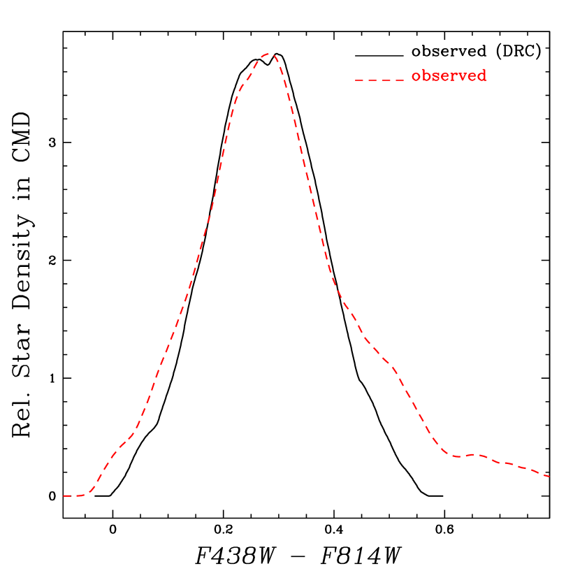
Figure 6: Comparison between the colour distributions obtained from the differential-reddening-corrected CMD (black solid line) and the observed CMD (red dashed line).

To further determine whether or not a single population can reproduce the observed CMD, we conducted Monte Carlo simulations of a synthetic cluster with the properties implied by the isochrone fitting (see G11a and G14 for a detailed description of the method adopted to produce these simulations). Briefly, to simulate a SSP with a given age and chemical composition, we populated an isochrone with stars randomly drawn using a Salpeter mass function and normalized to the observed (completeness-corrected) number of stars. To a fraction of these sample stars, we added a component of unresolved binary stars derived from the same mass function, using a flat distribution of primary-to-secondary mass ratios. The binary fraction was estimated by using as a template the part of the observed MS between the MSTO region and the TO of the background population in the magnitude range $22.5\la F438W\la 19.5$ (see Fig. 2). We derived that the value of the binary fraction that best fit the data is of $\simeq$ 25%. We estimated that the internal systematic uncertainty in the binary fraction is $\simeq$ 5%; for the purposes of this work, the results do not change significantly within 10% of the binary fraction. Finally, we added photometric errors that were derived using our artificial star tests. We derived three different sets of synthetic CMDs: one with a single SSP of age 300 Myr, and two combining two SSPs of different ages (one with SSPs with ages of 300 Myr and 380 Myr, and the other with ages of 300 Myr and 410 Myr, respectively). In the last two cases, we derived a set of simulations in which we changed the ratio of the number of stars in the two populations, from 10% to 90% of stars in the younger SSP, with a 5% step increase in each run.

To compare in detail the observed MSTO region with the simulated ones, we created “pseudo-age” distributions (see G11a for a detailed description). Briefly, pseudo-age distributions are derived by constructing a parallelogram across the MSTO, with one axis approximately parallel to the isochrones and the other approximately parallel to them (the adopted parallelogram is shown in Figure 5). The (F438W $-$ F814W, F438W) coordinates of the stars within the parallelogram are then transformed into the reference coordinate frame defined by the two axis of the parallelogram and the same procedure is applied to the isochrones tables to set the age scale along this vector. The pseudo-age distributions are calculated using the non-parametric Epanechnikov-kernel density function (Silverman, 1986), in order to avoid possible biases that can arise if fixed bin widths are used. Finally, a polynomial least-squares fit between age and the coordinate in the direction perpendicular to the isochrones yields the final pseudo-age distributions. The described procedure is applied both to the observed and the simulated CMD. In the following sections, we describe the results obtained from the comparison of the observed and simulated pseudo-age distributions, for the synthetic CMDs obtained with a single SSP and for those obtained from the combination of two SSPs of different ages.

4.1 Comparison with the synthetic CMD of a SSP

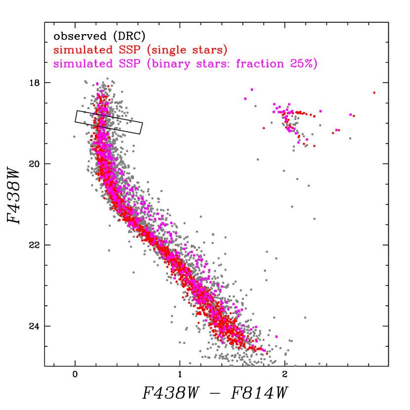
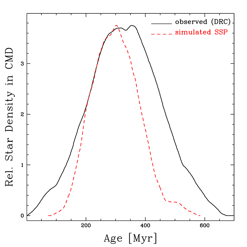
Figure 7: Top panel: comparison between DRC (gray dots) and simulated CMDs (red circles, single stars, magenta square, binary stars, respectively). The simulated CMD is obtained from Monte Carlo simulation of a SSP with an age of 300 Myr. The parallelogram box used to select MSTO stars and the fraction of the adopted binary stars are also reported. Bottom panel: Pseudo-age distribution for the MSTO region of the DRC (black solid line) and simulated (red dashed line) CMDs.

The top panel of Figure 7 shows the comparison between the observed and simulated CMD, the latter obtained from a single SSP with an age of 300 Myr. Overall, the SSP simulation reproduces the CMD features quite well in the fainter portion of the cluster MS (i.e.; for F438W $\ga$ 20.5 mag). Conversely, we note that the MSTO region of the simulated SSP does not reproduce the observed MSTO region very well, in that the latter is wider than the former. Furthermore, the faint end of the RC also does not seem to be reproduced well by the simulated SSP in that the simulated luminosity function of RC stars peaks more strongly at bright magnitudes than the observed one. Note that this is consistent with a fraction of stars in NGC 1856 having “older” ages than that of the best-fit SSP (see for reference the shape and location of the RC for the older isochrone in Figure 5). This difference is even more evident in a comparison of the observed and simulated pseudo-age distributions (see bottom panel of Figure 7). Indeed, the observed pseudo-age distribution (shown as a black solid line in Figure 7) reaches significantly older ages than the simulated one (red dashed line in Figure 7), while the two distributions are very similar to each other in the left (“young”) half of the respective profiles.

To quantify the difference between the pseudo-age distribution of the cluster data and that of the SSP simulation in term of intrinsic MSTO width of the cluster, we measured the widths of the two sets of distributions at 50% of their maximum values (hereafter called FWHM), using quadratic interpolation. The intrinsic pseudo-age range of the cluster is then estimated by subtracting the simulation width in quadrature:

$${\it FWHM}_{\rm MSTO}=({\it FWHM}^{2}_{\rm obs}-{\it FWHM}^{2}_{\rm SSP})^{1/2}$$ (2)

where the “obs” subscript indicates a measurement on the DRC CMD and the “SSP” subscript indicates a measurement on the simulated CMD for the SSP. With ${\it FWHM}_{\rm obs}$ = 269 Myr and ${\it FWHM}_{\rm SSP}$ = 198 Myr, we obtain ${\it FWHM}_{MSTO}\approx$ 182 Myr, which is similar to the value of ${\it FWHM}_{\rm SSP}$. This suggests that NGC 1856 may host two SSPs separated in age by about ${\it FWHM}_{MSTO}/2\sim$ 90 Myr (see Sect. 4.2 below).

In this context, we adopted equation 2 also to derive the value of reddening variation necessary to reproduce the observed pseudo-age distributions assuming that a cluster is formed by a SSP. Instead of age, we derived the FWHM of the observed and simulated pseudo-age distributions as a function of F438W - F814W; using the appropriate extinction coefficient for the UVIS WFC3 filters we transformed the “$\Delta$ color” in $\Delta A_{V}$ obtaining the following value: $\Delta A_{V}$ = 0.27. The derived $\Delta A_{V}$ is significantly larger than the reddening variations observed in the spatial differential reddening map in the innermost region of the cluster. Moreover, we note that due to the uniform shape of the observed pseudo-age distribution, this large reddening should affect a significant number of stars, making the possibility that the reddening can mimic the presence of a multiple population even less plausible. Therefore, taking these results at face value, they seem to suggest that a SSP is not able to reproduce the observed morphology of the MSTO region.

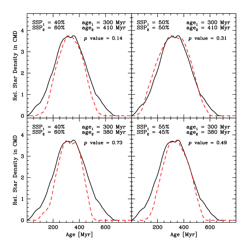
Figure 8: Comparison between the observed pseudo-age distribution (from the DRC CMD, black solid line) and the ones obtained from the combination of two SSPs with different ages (300 Myr and 410 Myr, top panels; 300 Myr and 380 Myr, bottom panels) shown as red dashed lines. In each panel we report the adopted ages of the two SSPs and the number ratio between the younger SSP and the old one. Two-tail p values obtained for the K-S test are also shown.

4.2 Comparison with a synthetic CMD of two SSPs of different age

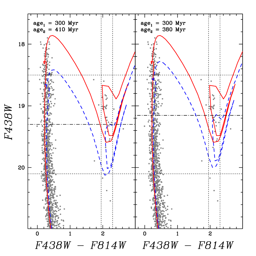
Figure 9: Left panels: DRC CMDs zoomed in the upper portion of the MS with superimposed isochrones (red solid and blue dashed lines for the young and the old isochrones, respectively) from Marigo et al. (2008) along with the adopted ages (left panel: 300 and 410 Myr. Right panel: 300 and 380 Myr). Dotted lines represent the magnitude and colour cuts adopted to select RC stars, whereas the dotdashed lines represent the magnitude cut, used to divide the two parts of the RC. Right panels: ratios between the stars in the upper portion of the RC and their total number as a function of the ratio of the young SSP (top panel: SSPs with ages of 300 and 410 Myr; bottom panel: SSPs with ages of 300 Myr and 410 Myr). The ratio obtained in the observed DRC CMD is reported as a dashed line in both panels. The typical uncertainty ($\approx$ 10%) in the calculated number ratio is also shown.

As stated in Section 4, we also simulated synthetic CMDs combining two SSPs with different ages. One set is obtained using SSPs with ages of 300 Myr and 410 Myr and the other with ages of 300 Myr and 380 Myr. For both cases, we derived a set of simulations in which we varied the ratio of the number of stars in the young and the old SSP, from 10% to 90% in each of them, with a step of 5%. For each simulated CMD we obtained the corresponding pseudo-age distribution that we compared with the observed one.

The fact that the stars from the two SSPs are mixed together in the parallelogram used to derive the pseudo-age distribution, combined with our purely statistical approach, cause an increase in the “free parameters” and introduces a sort of degeneracy in the derived results. This is reflected in the fact that we obtained more than one simulated pseudo-age distribution that reasonably reproduces the observed one. These “best-fitting” pseudo-age distributions are shown in Figure 8. In detail, the top panels show the best fit achieved from the SSPs with ages of 300 Myr and 410 Myr (with mass fractions of “young” stars of 40% and 50%, respectively), whereas in the bottom panels we show the ones obtained from the SSPs with ages of 300 Myr and 380 Myr (with mass fractions of young stars of 40% and 55%, respectively) The ages of the two SSPs and the ratio between them have been reported in each panel. We note that the best-fit mass ratios of the young to the old population seem to be around 1:1, consistent with the observed pseudo-age distribution, where we see a hint of two peaks with a similar maximum value and hence a likely number ratio of $\approx$ 1:1 for young vs. old stars in the cluster.

To constrain which combination of two SSPs provides the best solution to reproduce the observed CMD of NGC 1856, we performed two-sample Kolmogorov-Smirnov (K-S) tests. The two-tailed p values are mentioned in Figure 8 for each pseudo-age distribution. Taking these results at face value, it seems that the combination of SSPs with ages of 300 and 380 Myr provide a better solution with respect to the SSPs with ages of 300 and 410 Myr. To further constrain the two-SSP fits, we pointed our attention to the distribution of RC stars, adopting the following approach. The left panels of Figure 9 show the DRC CMDs zoomed in to the RC and the upper portion of the MS, with superimposed isochrones from Marigo et al. (2008), with the same ages as those adopted in the SSPs (left sub-panel: 300 and 410 Myr; right sub-panel: 300 and 380 Myr, respectively). First, we selected cluster RC stars by applying colour and magnitude cuts (shown as dotted lines in the left panels of Figure 9). Then, we divide RC stars in two parts, applying a magnitude threshold (shown as dotdashed lines in Figure 9) coinciding with the brightest point of the RC of the “old” isochrone (i.e., F438W = 19.3 mag for the 410 Myr isochrone and F438W = 19.15 mag for the 380 Myr isochrone). Finally, we counted the stars in the upper and lower portion of the RC, both in the observed data and in each synthetic CMD obtained from the associated Monte Carlo simulations.

The ratios between the stars in the upper portion of the RC and their total number as a function of the mass ratio of the young SSP in each simulation are shown in the right panels of Figure 9 (for SSPs with ages of 300 Myr and 410 Myr in the top panel and for SSPs with ages of 300 Myr and 380 Myr in the bottom panel, respectively). The ratios from the DRC CMD, obtained with the different magnitude cuts, are shown as dashed lines. The typical uncertainty on the mass ratios has been estimated to be of order 10%, shown as an error bar in both panels. Taking these results at face value, it seems that the best match is obtained from the synthetic CMD obtained from the SSPs with ages of 300 Myr and 380 Myr and with a fraction of young stars of 0.55 $\pm$ 0.10 (cf. bottom right panel in Figure 8).

Globally, the results presented in Section 4.1 and 4.2 show that a single SSP fails in reproducing the observed pseudo-age distribution while a combination of two SSPs with different ages can provide a very good fit. This seems to indicate that a spread in age may be present in the cluster and can not be categorically excluded as argued by Bastian & Silva-Villa (2013).

5 Constraints on ongoing star formation activity

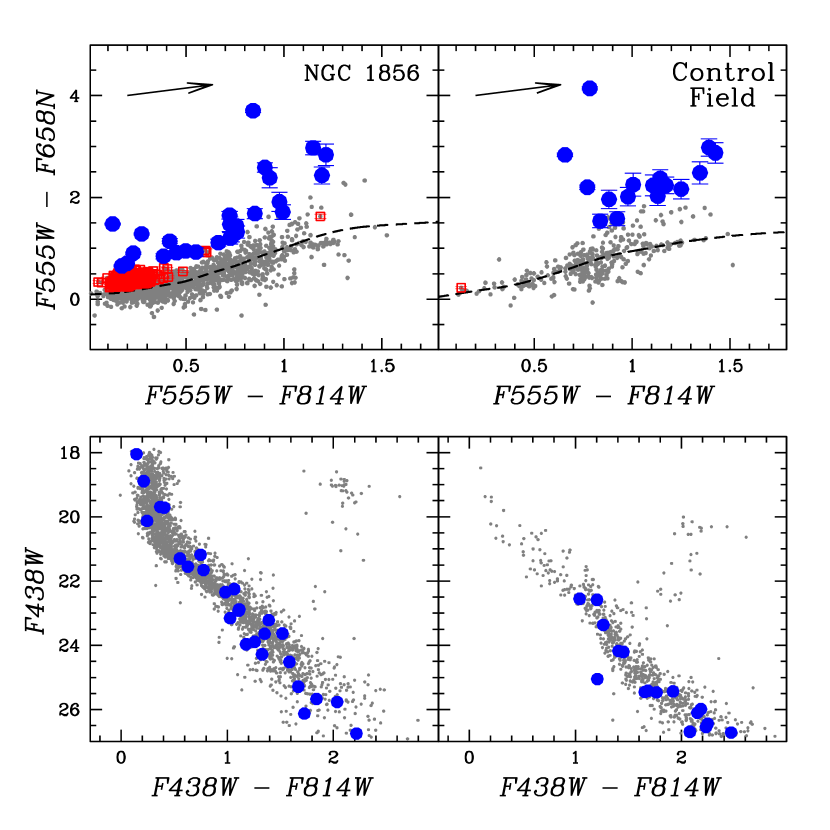
Figure 10: Top panels: F555W - F814W vs F555W - F658N colour-colour diagram for the stars inside the core radius (left panel) and in the control field (right panel), representing the contamination from the background LMC stars (same field adopted in Figure 2). The dashed line represents the median F555W - F658N colour, representative of stars with no $H_{\alpha}$ excess. Stars with a F555W - F658N colour at least $5\sigma$ above that reference line, where $\sigma$ is the uncertainty on the F555W - F658N colour of the star, are reported as open red squares. Those among them with $EW_{H_{\alpha}}>10\AA$, where the equivalent width of the $H_{\alpha}$ emission line ($EW_{H_{\alpha}}$) is calculated using the Eq. 4 of De Marchi et al. (2010) are reported as solid blue circles. Bottom Panels: CMDs of the cluster and of the control field with overplotted stars selected from the F555W - F814W vs F555W - F658N colour-colour diagram (solid blue circles).

To study whether NGC 1856 presently hosts ongoing star formation, we performed a search for PMS stars by means of narrow-band imaging of the H$\alpha$ line. H$\alpha$ emission is a good indicator of the PMS stage: the presence of strong H${\alpha}$ emission ($EW_{H{\alpha}}>10$ Å) in young stellar objects is normally interpreted as a signature of the mass accretion process onto the surface of the object that requires the presence of an inner disk (see Feigelson & Montmerle, 1999; White & Basri, 2003, and reference therein). To do this, we used the method described in De Marchi et al. (2010), which combines V and I broad-band photometry with narrow-band $H{\alpha}$ imaging to identify all the stars with excess $H{\alpha}$ emission and to measure their $H{\alpha}$ luminosity.

In the top panels of Figure 10 we show the F555W $-$ F814W vs. F555W $-$ F658N colour-colour diagram for the stars inside the cluster core radius (left top panel) and for the stars in the “control field”, the same field we used to derive the contamination by the background LMC population in Figure 2 (right top panel). We used the median F555W $-$ F658N colour of stars with small ($<$ 0.05 mag) photometric uncertainties in each of the three F555W, F814W, and F658N bands, as a function of F555W $-$ F814W, to define the reference template with respect to which excess $H{\alpha}$ emission is identified (shown by the dashed line in Figure 10). We selected a first candidate sample of stars with $H{\alpha}$ excess emission by considering all those with a F555W $-$ F658N color at least $5\sigma$ above that reference line, where $\sigma$ is the uncertainty on the F555W $-$ F658N colour of the star in question (shown as open red squares in Figure 10). Then we calculated the equivalent width of the $H{\alpha}$ emission line ($EW_{H{\alpha}}$) from the measured color excess, using the following equation from De Marchi et al. (2010):

$$W_{eq}(H{\alpha})=RW\times[1-10^{-0.4\times(H{\alpha}-H{\alpha}^{c})}]$$ (3)

where RW is the rectangular width of the filter (similar in definition to the equivalent width of the line), which depends on the characteristic of the filter (for the adopted F658N filter, Rw = 17.68; see Table 4 in De Marchi et al., 2010). Finally, we considered as bona-fide candidate PMS stars those objects with $EW_{H{\alpha}}>10$ Å  (White & Basri, 2003), shown as solid blue circles in Figure 10. The number of objects that show excess $H{\alpha}$ emission is very low and is roughly the same in both fields. In the bottom panels of Figure 10, we overplotted these objects (shown as solid blue circles) on the F438W $-$ F814W vs. F438W CMDs of the cluster and the control field; the majority of them are located on the fainter part of the CMD, where the photometric errors are larger and the contamination by background LMC stars is higher. In fact the number of objects that show an $H{\alpha}$ excess is comparable within the errors in the two fields below the TO of the background stellar population (i.e. F438W $\la$ 23 mag). Hence, the number and the location of these objects in the CMDs suggest that they can be considered spurious detections. For what concerns the handful of objects at brighter magnitudes (i.e. F438W $\ga$ 22 mag), where the photometric errors are smaller and the contamination is lower, we hypothesize that these can be stars in a binary system in which mass transfer between the primary and the secondary star is occurring. We exclude the possibility that these objects are true PMS stars due to the fact that, in this case, we would have observed a significant number of these objects at fainter magnitudes (i.e. lower masses and hence longer PMS lifetime).

In this context, it is worth to note that our magnitude detection limit for stars showing $H{\alpha}$ excess is around F438W $\simeq$ 26.5 mag, which, at the cluster age, corresponds to stars with masses of $\simeq$ 0.8 M_⊙. The PMS lifetime for such stars is of the order of $\sim$ 120 Myr, indicating that if star formation is occuring within the cluster, with our method we should be able to observe a significant number of PMS objects.

Hence, these results indicate that the level of ongoing star formation activity is negligible in NGC 1856. In fact, the lack of low-mass stars showing an $H{\alpha}$ excess indicates that the star formation in the cluster must have stopped at least $\sim$ 120 Myr ago, in agreement with the conclusions derived from the pseudo-age distribution analysis.

6 Constraints to the stellar rotation scenario in producing eMSTO’s

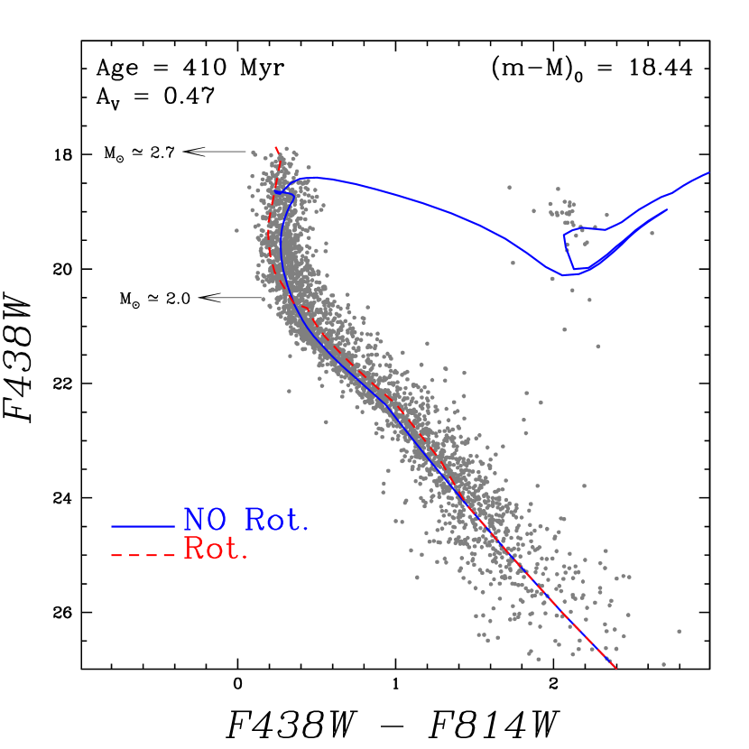
Figure 11: Comparison between the non-rotating isochrone (blue solid line), from Marigo et al. (2008), and its rotating counterpart (rec dashed line), derived as described in Section 6. Isochrones are superposed on the cluster DRC CMD, along with adopted age, distance modulus $(m-M)_{0}$ and visual extinction $A_{V}$.

In the literature, some alternative explanations that do not invoke the presence of an extended star formation, have been proposed to explain the eMSTO phenomenon in intermediate-age star clusters. In particular, the so called “stellar rotation” scenario (Bastian & de Mink, 2009; Yang et al., 2013) suggest that eMSTOs can be explained by a spread in rotation velocity among turn-off stars. Yang et al. (2013) calculated evolutionary tracks of non-rotating and rotating stars for three different initial stellar rotation periods (approximately 0.2, 0.3 and 0.4 times the Keplerian rotation of ZAMS stars), and for two different rotational mixing efficiencies (“normal”, $f_{c}=0.03$ and “enhanced”, $f_{c}=0.20$). From the isochrones, built from these tracks, they calculated the widths of the MSTO region caused by stellar rotation as a function of cluster age and translated them to age spreads. In particular, Figure 7 in Yang et al. (2013) shows the equivalent width of the MSTO of star clusters caused by rotation as a function of the cluster age, for different initial stellar rotation periods and rotational mixing efficiencies. At the age of NGC 1856, all the Yang et al. models with “normal” mixing efficiency (i.e.; $f_{c}=0.03$) indicate that rotation does not cause any appreciable spread. On the other hand, for their models with “enhanced” mixing efficiency (i.e.; $f_{c}=0.20$), the predictions vary from no spread for the model with the longest initial stellar rotation period to a maximum of $\sim$ 100 Myr for the model with the shortest period (i.e., the model for the highest rotation velocity). In this case their model predicts a “negative” spread, in the sense that the rotating model exhibits a bluer MSTO with respect to their non-rotating counterpart, thus mimicking the presence of a younger population (see top left panel of Figure 6 in Yang et al., 2013).

To test the prediction of this rotating model in the specific case of NGC 1856, we used the 410 Myr isochrone from Marigo et al. (2008) as a template for non-rotating stars (i.e., the same isochrone as that plotted in Figure 5), and we derived its rotating counterpart. To do so, we calculated the shifts in colour and magnitude between the rotating and non-rotating isochrones in Figure 6 of Yang et al. (2013), we then transformed these shifts in our photometric system and we applied them to the Marigo et al. (2008) isochrone. Figure 11 shows the DRC CMD of NGC 1856 with superimposed non-rotating and rotating isochrones (blue solid and red dashed line, respectively). For the rotating isochrone, we plotted only the MS part, since the post-MS era of stellar evolution is not addressed by the Yang et al. (2013) models. Overall, the rotating model plotted in Figure 11 seems to reproduce the observed CMD reasonably well in the upper portion of the MS, whereas the bottom portion of the MS is not as well reproduced, the rotating model being somewhat too red with respect to the observed MS. The latter is due to the fact that the rotating model bends toward red colors (lower temperatures) for stellar masses ${\cal{M}}\la$ 2.0 M_⊙.

In conclusion, the rotating model of Yang et al. (2013) that involves “enhanced” rotational mixing efficiency seems to provide a satisfactory fit to the observed MS of NGC 1856, indicating that a spread in rotation velocity, beside an age spread, could be a possible cause of the observed broadening of the MSTO region. However, we note that the predictions of the Yang et al. (2013) models are not consistent with the observations for intermediate-age ($\sim$  1– 2 Gyr) star clusters featuring eMSTOs. This is especially the case for the rotating models involving enhanced rotational mixing efficiency (see discussion in G14, in particular their Figure 7). It should however also be recognized that the study of the creation of theoretical stellar tracks and isochrones for rotating stars at various stages of stellar evolution, rotation rates, and ages is still in relatively early stages. To date, no stellar rotation velocity measurements have yet been undertaken in young and intermediate-age star clusters in the Magellanic Clouds. We strongly encourage such studies in the future in order to provide fundamental improvements of our understanding of the possible relation between the eMSTO phenomenon and the effects of stellar rotation.

7 Insights from Dynamical Analysis

As mentioned in the Introduction, a peculiar characteristic of eMSTOs in intermediate-age star clusters in the Magellanic Clouds is that they are not hosted by all such star clusters. To explain this phenomenon in the context of multiple stellar populations, G11a proposed a scenario in which eMSTOs can only be hosted by clusters for which the escape velocity of the cluster is higher than the wind velocities of “polluter” stars thought to provide the material out of which the second stellar generation is formed, at the time such stars were present in the cluster (we refer to this as “the escape velocity threshold” scenario). This scenario was developed further by G14 who studied HST photometry of a sample of 18 intermediate-age (1 – 2 Gyr) star clusters in the Magellanic Clouds that covered a variety of masses and core radii. They found that all the clusters showing an eMSTO feature escape velocities $V_{\rm esc}\ga$ 15 km s^-1 out to ages of at least 100 Myr. This age is equivalent to the lifetime of stars of $\approx 5\;M_{\odot}$ (e.g., Marigo et al., 2008), and hence old enough for the slow winds of massive binary stars and IM-AGB stars of the first generation to produce significant amounts of “polluted” material out of which second-generation stars may be formed. Furthermore, C14 showed that this threshold on $V_{\rm esc}$ is consistent with HST observations of four low-mass intermediate-age star clusters ($\approx 10^{4}\;M_{\odot}$): the two clusters that host eMSTOs have $V_{\rm esc}\ga$ 15 km s^-1 out to ages of $\sim$ 100 Myr, whereas $V_{\rm esc}\la$ 12 km s^-1 at all ages for the two clusters not exhibiting eMSTOs. Hence, the critical escape velocity for a star cluster to be able to retain the material ejected by first-generation polluter stars seems to be in the range of 12 – 15 km s^-1. This threshold is consistent with wind velocities of IM-AGB stars and massive binary stars (see G14 for a detailed discussion). Briefly, IM-AGB stars show wind velocities in the range 12 – 18 km s^-1(Vassiliadis & Wood, 1993; Zijlstra et al., 1996), whereas observed velocities of ejecta of massive binary stars are in the range 15 – 50 km s^-1(Smith et al., 2002, 2007).

With this in mind, following the results presented in the previous sections where the analysis of pseudo-age distributions seems to suggest the presence of multiple stellar populations in NGC 1856, we determined the structural parameters and the dynamical properties of the cluster from our new HST/WFC3 data.

7.1 Structural parameters

Figure 12: Radial surface number density profile of NGC 1856. Black points represent observed values. The dashed line represents the best-fit King model (cf. equation 4) whose parameters are shown in the legend. Ellipticity and effective radius $r_{e}$ are also shown in the legend. The radius values have been converted to parsec by adopting the appropriate distance modulus.

We determined the radial surface number density distribution of stars, following the procedure described in Goudfrooij et al. (2009). Briefly, we first determined the cluster centre to be at reference coordinate ($x_{c}$, $y_{c}$) = (2986, 1767) with an uncertainty of $\pm$ 5 pixels in either axis. In order to derive it, we first created a two-dimensional histogram of the pixel coordinates adopting a bin size of 50 $\times$ 50 pixels and then calculated the centre using a two-dimensional Gaussian fit to an image constructed from the surface number density values in the aforementioned two-dimensional histogram. This method avoids possible biases related to the presence of bright stars near the centre. We derived the cluster ellipticity $\epsilon$ running the task ellipse within IRAF/STSDAS on the surface number density images. Finally, we derived radial surface number densities by dividing the area sampled by the images in a series of elliptical annuli, centered on the cluster, and accounting for the spatial and photometric completeness in each annulus.

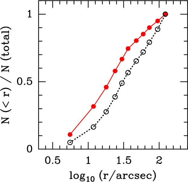
Figure 13: Cumulative completeness-corrected radial distribution of bright versus faint stars. Red solid circles and solid line represent stars with F438W $<$ 20.5 mag while black open circles and dotted line represent stars with 21.0 $<$ F438W $<$ 23.5 mag.

We only considered stars brighter than the 30% completeness limit in the core region, corresponding to F438W $\leq$ 23.5 mag. The outermost data point is derived from the ACS parallel observations in a field located $\simeq$ 5$\aas@@fstack{\prime}$5 from the cluster centre. The radial surface number density profile was fitted using a King (1962) model combined with a constant background level, described by the following equation:

$$n(r)=n_{0}\>\left(\frac{1}{\sqrt{1+(r/r_{c})^{2}}}-\frac{1}{\sqrt{1+c^{2}}}\right)^{2}\;+\;{\rm bkg}$$ (4)

where $n_{0}$ is the central surface number density, $r_{c}$ is the core radius, $c\equiv r_{t}/r_{c}$ is the King concentration index ($r_{t}$ being the tidal radius), and $r$ is the geometric mean radius of the ellipse ($r=a\,\sqrt{1-\epsilon}$, where a is the semi-major axis of the ellipse). In Figure 12, we show the best-fit King model, obtained using a $\chi^{2}$ minimization routine. We reported also the derived number density values along with other relevant parameters. Our derived core radius of $r_{c}$ = 3.18 ($\pm$ 0.12) pc is significantly larger than the literature value for NGC 1856 ($r_{c}$ = 1.14 pc, McLaughlin & van der Marel, 2005). In reconciling this difference, we note that our King-model fit was done using completeness-corrected surface number densities, whereas McLaughlin & van der Marel (2005) used surface brightness data to derive the structural parameters of the cluster. The latter method is sensitive to the presence of mass segregation in the sense that mass-segregated clusters will appear to have smaller radii when using surface brightness data than when using plain surface number densities. To check whether NGC 1856 is actually mass segregated, we derived the cumulative completeness-corrected radial distribution of bright and faint stars in the WFC3 image. “Bright” stars are selected by the magnitude cut F438W $<$ 20.5 mag, whereas “faint” stars are selected in the magnitude range 21.0 $<$ F438W $<$ 23.5 mag. The obtained cumulative radial distributions are shown in Figure 13. Note that the bright stars are clearly more centrally concentrated than the faint ones, confirming that a significant degree of mass segregation is present in the cluster.

7.2 Dynamical evolution and cluster escape velocity

V	Aper.	Aper. corr.	[Z/H]	$A_{V}$	Age	$r_{c}$	$r_{e}$
(1)	(2)	(3)	(4)	(5)	(6)	(7)	(8)
10.06 $\pm$ 0.15	31	0.38	$-$0.30	0.47	300	3.18 $\pm$ 0.12	8.00 $\pm$ 0.90

Table 2: Physical properties of the star cluster. Columns (1): Integrated-light $V$ magnitude from Bica et al. (1996). (2): Aperture radius in arcsec used for the integrated-light measurement. (3): Aperture correction in mag. (4): Metallicity in dex. (5): Visual extinction in magnitude. (6): Mean age in Myr. (7): Core radius in pc. (8): Effective radius in pc.

log (${\cal{M}}_{\rm cl}/M_{\odot}$)			$V_{\rm esc}$ (km s-1)
Current	107 yr w/o m.s.	107 yr with m.s.	Current	107 yr w/o m.s.	107 yr with m.s.	107 yr “plausible”
(1)	(2)	(3)	(4)	(5)	(6)	(7)
5.07 $\pm$ 0.07	5.15 $\pm$ 0.10	5.37 $\pm$ 0.10	11.4 $\pm$ 0.7	13.7 $\pm$ 0.7	20.0 $\pm$ 0.7	17.1 $\pm$ 0.8

Table 3: Dynamical properties of the star cluster. Columns (1): Logarithm of the adopted current cluster mass. (2-3): Logarithm of the adopted cluster mass at an age of 10⁷ yr without(with) the inclusion of initial mass segregation. (4): Current cluster escape velocity at the core radius. (5-6): Cluster escape velocity at the core radius at an age of 10⁷ yr without(with) the inclusion of initial mass segregation. (8) “Plausible” cluster escape velocity at an age of 10⁷ yr.

We estimated the cluster mass and escape velocity as a function of time, going back to an age of 10 Myr, after the cluster has survived the era of violent relaxation and when the most massive stars of the first generation, proposed to be candidate polluters in literature (i.e., FRMS and massive binary stars), are expected to start losing significant amounts of mass through slow winds. The current mass of NGC 1856 was determined from its integrated-light V-band magnitude listed in Table 2. We determined the aperture correction for this magnitude from the best-fit King model derived in Sect. 7.1 by calculating the fraction of total cluster light encompassed by the measurement aperture. After correcting the integrated-light V magnitude for the missing cluster light beyond the measurement aperture, we calculated the total cluster mass adopting the values of $A_{V},\mbox{[Z/H]}$, and age listed in Table 2. This was done by interpolation between the ${\cal{M}}/L_{V}$ values in the SSP model tables of Bruzual & Charlot (2003), assuming a Salpeter (1955) initial mass function. The latter models were recently found to provide the best fit (among popular SSP models) to observed integrated-light photometry of LMC clusters with ages and metallicities measured from CMDs and spectroscopy of individual stars in the 0.2 – 1 Gyr age range (Pessev et al., 2008).

We calculated the dynamical evolution of the star cluster following the prescriptions of G14. Briefly, the evolution of cluster mass and radius was evaluated with and without initial mass segregation, given the fundamental role that the latter property plays in terms of the early evolution of the cluster’s expansion and mass loss rate (e.g., Mackey et al., 2008b; Vesperini et al., 2009). For the case of a model cluster with initial mass segregation, we adopted the results of the simulation called SG-R1 in D’Ercole et al. (2008), which involves a tidally limited model cluster that features a level of initial mass segregation of $r_{e}/r_{e,>1}$ = 1.5, where $r_{e,>1}$ is the effective radius of the cluster for stars with ${\cal{M}}>$ 1 M_⊙(see G14 for a detailed description of the reasons for this choice).

Table 3 lists the derived masses and escape velocities at an age of 10 Myr, obtained with and without initial mass segregation. Escape velocities are calculated from the reduced gravitational potential $V_{\rm esc}(r,t)=(2\Phi_{\rm tid}(t)-2\Phi(r,t))^{1/2}$, at the core radius. Here $\Phi_{\rm tid}$ is the potential at the tidal (truncation) radius of the cluster. The choice to calculate the escape velocity at the cluster core radius is related to the prediction of the “in situ” scenario, where the second-generation stars are formed in the innermost region of the cluster (D’Ercole et al., 2008). For convenience, we define $V_{\rm esc,7}(r)\equiv V_{\rm esc}\,(r,t=10^{7}{\rm yr})$, and refer to it as “early escape velocity”. To estimate “plausible” values for $V_{\rm esc,\,7}$ we used a procedure that involves various results from the compilation of Magellanic Cloud star cluster properties and N-body simulations by Mackey et al. (2008b). Briefly, they showed that the maximum core radius seen among a large sample of Magellanic Cloud star clusters increases approximately linearly with log(age) up to an age of $\sim$ 1.5 Gyr, namely from $\simeq$ 2.0 pc at $\simeq$ 10 Myr to $\simeq$ 5.5 pc at $\simeq$ 1.5 Gyr. Conversely, the minimum core radius is $\sim$ 1.5 pc throughout the age range 10 Myr – 2 Gyr. Using N-body modeling Mackey et al. (2008b) showed that this behavior is consistent with adiabatic expansion of the cluster core in clusters with different levels of initial mass segregation, in that clusters with the highest level of mass segregation experience the strongest core expansion (see G14 for a more detailed discussion). Under this assumption, we derive that the “plausible” early escape velocity for NGC 1856 is $V_{\rm esc}=17.1\pm 0.8$ km s^-1, high enough to retain material shed by the slow winds of the polluters stars.

Figure 14 shows the escape velocity of NGC 1856 as a function of age, derived based on the assumed level of mass segregation presented above. The critical escape velocity range of 12 – 15 km s^-1 derived by C14 and G14 is depicted as the light grey region in Figure 14. The region below 12 km s^-1, representing, as stated above, the velocity range in which eMSTOs are not observed in intermediate-age star clusters (C14), is shown in dark grey. We note that $V_{\rm esc}$ for NGC 1856 is $\ga 14-15$ km s^-1 out to an age of $\approx$ 100 Myr. We recall that this is equivalent to the lifetime of stars of $\approx 5\;M_{\odot}$ (i.e., IM-AGB stars, see Ventura & D’Antona 2009) so that the slow winds of massive binary stars and IM-AGB stars of the first generation should have produced significant amounts of “polluted” material within that time. As mentioned above, this situation is similar to that shared among eMSTO clusters of intermediate age in the Magellanic Clouds (G14). It thus seems plausible that a significant fraction of that material may have been retained within the potential well of NGC 1856, allowing second-generation stars to be formed.

Finally, we note that the mass and escape velocities of NGC 1856 were likely high enough for the cluster to be able to accrete a significant amount of “pristine” gas from its surroundings in the first several tens of Myr after its birth. This would have constituted an additional source of gas to form second-generation stars (Conroy & Spergel 2011; G14; but see also Bastian & Strader 2014).

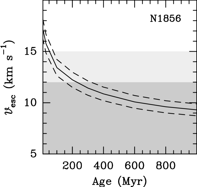
Figure 14: Escape velocity $V_{\rm esc}$ as a function of time. The light grey region represents the critical range of $V_{\rm esc}$ mentioned in Sect. 7, i.e., 12 – 15 km s^-1. The region below 12 km s^-1, in which $V_{\rm esc}$ is thought to be too low to permit retention of material shed by the first stellar generation, is shown in dark grey. $\pm 1\sigma$ errors of $V_{\rm esc}$ are shown by dashed lines.

8 Summary and Conclusion

We presented results obtained from a study of new, deep HST/WFC3 images of the young (age $\simeq$ 300 Myr) massive star cluster NGC 1856 in the LMC. After correction for differential reddening, we compared the CMD of the cluster with Monte Carlo simulations, both of one “best-fit” SSP and of two SSPs of different ages, in order to investigate the MSTO morphology and to quantify the intrinsic width of the MSTO region of the cluster. We studied the physical and dynamical properties of the cluster, deriving its radial surface number density distribution and determining the evolution of cluster mass and escape velocity from an age of 10 Myr to 1 Gyr, considering the possible effects of initial mass segregation.

The main results of the paper can be summarized as follows:

• NGC 1856 shows a broad MSTO region whose width can not be explained by photometric uncertainties, LMC field star contamination, or differential reddening effects. Comparison with Monte Carlo simulations of a SSP shows that the observed pseudo-age distribution is significantly wider than that derived from a single-age simulation. Conversely, combining two SSPs with different ages, we obtain a set of pseudo-age distributions that reproduce the observed one quite well. By considering the luminosity function of the RC feature, we conclude that a best fit is achieved with a combination of SSPs with ages of 300 Myr and 380 Myr and a mass fraction for the younger component of $\approx$ 55%. The observed pseudo-age distribution shows two distinct peaks with a similar maximum value and an uniform decline towards younger and older ages, with respect to the peaks. However, the small separation in age between the two peaks prevents us to conclude whether the morphology of the MSTO can be better explained with a smooth spread in age or by two discrete bursts of star formation. These results do not agree with the conclusions of Bastian & Silva-Villa (2013) who conclude that the CMD of NGC 1856 is consistent with a single age to within 35 Myr. We expect that this difference is due to the fact that our data are significantly deeper, namely $\sim$ 6 mag. Consequently, we suggest that the arguments of Bastian & Silva-Villa (2013) against the “age spread” scenario should be considered with caution.

• We use $V$, $I$, and H$\alpha$ images to select and study candidate (“putative”) pre-MS stars in NGC 1856. The numbers of “putative” pre-MS stars in the cluster field and the control (background) field are found to be similar, suggesting that the detections can be considered spurious and/or associated to residual noise. This indicates that star formation is not currently ongoing in the cluster.

• The “stellar rotation” scenario for the nature of the eMSTO phenomenon has been tested by evaluating rotating and non-rotating isochrones of the same age with the DRC CMD. Overall, a reasonable range of rotation velocities seems to be able to reproduce the MSTO properties quite well, albeit only if the rotational mixing efficiency is significantly higher than typically assumed values. However, several properties of MSTOs and RCs among eMSTO star clusters in the age range of 1 – 2 Gyr are inconsistent with such high rotational mixing efficiencies. This seems to indicate that a range of stellar ages provides a more likely explanation of the eMSTO phenomenon (including the wide MSTO of NGC 1856) than does a range of stellar rotation velocities, altough, with the current data alone, the latter hypothesis cannot formally be discarded. In this context, new stellar rotation measurements in young and intermediate-age star clusters, combined with new models of theoretical tracks and isochrones for rotating stars will be of fundamental importance to address the role of stellar rotation in the eMSTO phenomenon.

• The dynamical properties of NGC 1856 derived from our data suggest that the cluster has an early escape velocity of $\approx$ 17 km s^-1, high enough to permit the retention of material shed by the slow winds of polluter stars (IM-AGB stars and massive binary stars). The cluster escape velocity remains above the threshold value of 14 – 15 km s^-1 for $\approx$ 80 – 100 Myr, long enough for the slow winds of IM-AGB stars to have ejected their envelopes. This material would likely have been available for second-generation star formation which could have caused the wide MSTO. Furthermore, these early escape velocities are consistent with observed wind velocities of ejecta of IM-AGB stars and with those seen in massive binary star systems.

Appendix A Photometric Catalog

In Table 4 we report positions and magnitudes, with the associated errors, for the first ten objects in our final photometric catalog. The complete table of stellar photometry is available upon request.

ID	X	Y	F438W	err	F555W	err	F656N	err	F814W	err
(1)	(2)	(3)	(4)	(5)	(6)	(7)	(8)	(9)	(10)	(11)
1	1277.992	16.072	27.066	0.280	99	99	99	99	23.549	0.195
2	1279.163	19.076	99	99	27.625	0.262	22.958	0.317	99	99
3	1274.036	20.648	26.536	0.156	99	99	22.620	0.292	99	99
4	1300.449	22.857	27.221	0.289	99	99	22.664	0.239	99	99
5	1319.126	26.275	21.564	0.019	99	99	20.680	0.072	99	99
6	1296.704	26.879	27.217	0.377	99	99	22.607	0.315	99	99
7	1306.224	27.537	27.096	0.208	99	99	22.816	0.218	99	99
8	1269.086	28.177	27.537	0.248	99	99	23.518	0.462	99	99
9	1290.509	29.335	25.467	0.076	24.877	0.058	99	99	23.678	0.041
10	1278.772	31.292	24.668	0.059	24.051	0.045	99	99	23.047	0.034

Table 4: Stellar photometry. (1): Identification number. (2-3): X and Y coordinates in pixels. (4-11): magnitudes and associated errors.

References

- Bastian & de Mink (2009) Bastian, N., & de Mink, S. E. 2009, MNRAS, 398, L11
- Bastian & Silva-Villa (2013) Bastian, N., & Silva-Villa, E. 2013, MNRAS, 431, L21
- Bastian & Strader (2014) Bastian, N., & Strader, J. 2014, MNRAS, 443, 3594
- Bastian et al. (2013) Bastian, N., Lamers, H. J. G. L. M., de Mink, S. E., Longmore, S. N., Goodwin, S. P., & Gieles, M. 2013, MNRAS, 436, 2398
- Bica et al. (1996) Bica, E., Claría, J. J., Dottori, H., Santos, J. F. C., & Piatti, A. E. 1996, ApJS, 102, 57
- Bruzual & Charlot (2003) Bruzual, G. A., & Charlot, S. 2003, MNRAS, 344, 1000
- Cardelli et al. (1989) Cardelli, J. A., Clayton, G. C., & Mathis, J. S. 1989, ApJ, 345, 245
- Conroy & Spergel (2011) Conroy, C., & Spergel, D. N. 2011, ApJ, 726, 36
- Correnti et al. (2014) Correnti, M., Goudfrooij, P., Kalirai, J. S., Girardi, L., Puzia, T. H., & Kerber, L. 2014, ApJ, 793, 121
- D’Antona & Ventura (2007) D’Antona, F., & Ventura, P. 2007, MNRAS, 379, 1431
- Decressin et al. (2007) Decressin, T., Meynet, G., Charbonnel, C., Prantzos, N., & Ekstróm, S. 2007, A&A, 464, 1029
- de Mink et al. (2009) de Mink, S. E., Pols, O. R., Langer, N., & Izzard, R. G. 2009, A&A, 5007, L1
- D’Ercole et al. (2010) D’Ercole, A., D’Antona, F., Ventura, P., Vesperini, E., & McMillan, S. L. W. 2010, MNRAS, 407, 854
- D’Ercole et al. (2008) D’Ercole, A., Vesperini, E., D’Antona, F., McMillan, S. L. W., & Recchi, S. 2008, MNRAS, 391, 825
- De Marchi et al. (2010) De Marchi, G., Panagia, N., & Romaniello, M. 2010, ApJ, 715, 1
- Feigelson & Montmerle (1999) Feigelson, E. D., & Montmerle, T. 1999, ARA&A, 37, 363
- Fruchter & Hook (1997) Fruchter, A. S., & Hook R. N. 2002, PASP, 114, 144
- Glatt et al. (2008) Glatt, K. et al., 2008, AJ, 135, 1703
- Girardi et al. (2011) Girardi, L., Eggenberger, P., & Miglio, A. 2011, MNRAS, 412, L103
- Girardi et al. (2009) Girardi, L., Rubele, S., & Kerber, L. 2009, MNRAS, 394, L74
- Goudfrooij et al. (2009) Goudfrooij, P., Puzia, T. H., Kozhurina-Platais, V., & Chandar, R. 2009, AJ, 137, 4988
- Goudfrooij et al. (2011a) Goudfrooij, P., Puzia, T. H., Chandar, R., & Kozhurina-Platais, V. 2011, ApJ, 737, 4 (G11a)
- Goudfrooij et al. (2011b) Goudfrooij, P., Puzia, T. H., Kozhurina-Platais, V., & Chandar, R. 2011, ApJ, 737, 3 (G11b)
- Goudfrooij et al. (2014) Goudfrooij, P., et al. 2014, ApJ, 797, 35
- Kalirai et al. (2012) Kalirai, J. S., et al. 2012, AJ, 143, 11
- Keller et al. (2012) Keller, S. C., Mackey, A. D., & Da Costa, G. S. 2012, ApJ, 761, L5
- King (1962) King, I. 1962, AJ, 67, 471
- Li et al. (2012) Li, Z., Mao, C., Chen, L., & Zhang, Q. 2012, ApJL, 761, 22
- Mackey et al. (2008a) Mackey, A. D., Broby Nielsen. P., Ferguson, A. M. N., & Richardson, J. C. 2008, ApJ, 681, L17
- Mackey et al. (2008b) Mackey, A. D., Wilkinson, M. I., Davies, M. B., & Gilmore, G. F. 2008, MNRAS, 386, 65
- Marigo et al. (2008) Marigo, P., Girardi, L., Bressan, A., Groenewegen, M. A. T., Silva, L., & Granato, G. L. 2008, A&A, 482. 883
- McLaughlin & van der Marel (2005) McLaughlin, D. E., & van der Marel, R. P. 2005, ApJS, 161, 304
- Milone et al. (2009) Milone, A. P., Bedin, L. R., Piotto, G., & Anderson, J. 2009, A&A, 497, 755
- Milone et al. (2012) Milone, A. P., Piotto, G., Bedin, L. R., Cassisi, S., Anderson, J., Marino, A. F., Pietrinferni, A., & Aparicio, A. 2012, A&A, 537, 77
- O’Donnell (1994) O’Donnell, J. E. 1994, ApJ, 422, 158
- Pessev et al. (2008) Pessev, P. M., Goudfrooij, P., Puzia, T. H., & Chandar, R. 2008, MNRAS, 385, 1535
- Rubele et al. (2011) Rubele, S., Girardi, L., Kozhurina-Platais, V., Goudfrooij, P., & Kerber, L. 2011, MNRAS, 414, 2204
- Rubele et al. (2010) Rubele, S., Kerber, L., & Girardi, L. 2010, MNRAS, 403, 1156
- Silverman (1986) Silverman, B. W. 1986, in Density Estimation for Statistics and Data Analysis, Chap and Hall/CRC Press, Inc.
- Salpeter (1955) Salpeter, E. E. 1955, ApJ, 121, 161
- Smith et al. (2002) Smith, N., Gehrz, R. D., Stahl, O., Balick, B., & Kaufer, A. 2002, ApJ, 578, 464
- Smith et al. (2007) Smith, N., Bally, J., & Walawender, J., 2007, AJ, 134, 846
- Stetson (1987) Stetson, P. B. 1987, PASP, 99, 191
- Stetson (1994) Stetson, P. B. 1994, PASP, 106, 250
- Vassiliadis & Wood (1993) Vassiliadis, E. & Wood, P. R. 1993, ApJ, 413, 641
- Ventura & D’Antona (2009) Ventura, P., & D’Antona, F. 2009, A&A, 499, 835
- Vesperini et al. (2009) Vesperini, E., McMillan, S. L. W., & Portegies Zwart, S. 2009, ApJ, 698, 615
- White & Basri (2003) White, R. J., & Basri, G. 2003, ApJ, 582, 1109
- Yang et al. (2011) Yang, W., Meng, X., Bi, S., Tian, Z., Li, T., & Liu, K. 2011, ApJ, 731, L37
- Yang et al. (2013) Yang, W., Bi, S., Meng, X., & Liu, Z. 2013, ApJ, 776, 112
- Zijlstra et al. (1996) Zijlstra, A. A., Loup, C., Waters, L. B. M. F., Whitelock, P. A., van Loon, J. T., & Guglielmo, F., 1996, MNRAS, 279, 32