The Algorithm of Pipelined Gossiping

Abstract

A family of gossiping algorithms depending on a parameter permutation is introduced, formalized, and discussed. Several of its members are analyzed and their asymptotic behaviour is revealed, including a member whose model and performance closely follows the one of hardware pipelined processors. This similarity is exposed. An optimizing algorithm is finally proposed and discussed as a general strategy to increase the performance of the base algorithms.

1 Introduction

A number of distributed applications like, e.g., distributed consensus [15], or those based on the concept of restoring organs [4, 12] ($N$-modular redundancy systems with $N$-replicated voters—for instance, the distributed voting tool described in [3]), require a base service called gossiping [8, 1, 5].

Informally speaking, gossiping is a communication procedure such that every member of a set has to communicate a private value to all the other members. Gossiping is clearly an expansive service, as it requires a large amount of communication. Implementations of this service can have a great impact on the throughput of their client applications and perform very differently depending on the number of members in the set. This work describes a family of gossiping algorithms that depend on a combinatorial parameter. Three cases are then analyzed under the hypotheses of discrete time, of constant time for performing a send or receive, and of a crossbar communication system. It is shown how, depending on the pattern of the parameter, gossiping can use from $\hbox{O}(N^{2})$ to $\hbox{O}(N)$ time, $N$ being the number of communicating members. The last and best-performing case, whose activity follows the execution pattern of pipelined hardware processors, is shown to exhibit an efficiency constant with respect to $N$. This translates in unlimited scalability of the corresponding gossiping service. When performing multiple consecutive gossiping sessions, the throughput of the system can reach the value of $t/2$, $t$ being the time for sending one value from one member to another, or a full gossiping is completed every two basic communication steps.

The structure of the paper follows: first, in Sect. 2, a formal model for the family of algorithms is provided. The following three sections (Sect. 3, Sect. 4, and Sect. 5) introduce, analyze, and discuss three members of the family, showing in particular that one of them, whose behaviour resembles the one of pipelined hardware microprocessors, uses $\hbox{O}(N)$ time, $N$ being the number of employed nodes. An optimizing algorithm is then introduced in Sect. 6. Section 7 describes two applications of our algorithms. Finally Sect. 8 summarizes our contributions and draws a number of conclusions.

2 A Formal Model

Definition 1 (system)

Let $N>0$. $N+1$ processors are interconnected via some communication means that allows them to communicate with each other (for instance, by means of full-duplex point-to-point communication lines). Communication is synchronous and blocking. Processors are uniquely identified by integer labels in $\{0,\dots,N\}$; they will be globally referred to, together with the communication means, as “the system”.

Definition 2 (problem)

The processors own some local data they need to share (for instance, to execute a voting algorithm [12]). In order to share their local data, each processor needs to broadcast its own data to all others, via multiple sending operations, and to receive the $N$ data items owned by its fellows. This must be done as soon as possible. We assume a discrete time model—events occur at discrete time steps, one event at a time per processor. This is a special class of the general family of problems of information dissemination known as gossiping [8, 1, 5]. We will refer to this class as “the problem”.

Definition 3 (time step)

We assume the time to send a message and that to receive a message is constant. We call this amount of time a “time step”.

Definition 4 (actions)

On a given time step $t$, processor $i$ may be:

1. sending a message to processor $j,j\neq i$; this is represented in form of relation as $i\,S^{t}j$;

2. receiving a message from processor $j,j\neq i$; this is represented as $i\,R^{t}j$;

3. blocked, waiting for messages to be received from any processor; where both the identities of the involved processors and $t$ can be omitted without ambiguity, symbol “$-$” will be used to represent this case;

4. blocked, waiting for a message to be sent i.e., for a designee to enter the receiving state; under the same assumptions of case (3), symbol “$\curvearrowright$” will be used.

The above cases are referred to as “the actions” of a time step.

Definition 5 (slot, used slot, wasted slot)

A slot is a temporal “window” one time step long, related to a processor. On each given time step there are $N+1$ available slots within the system. Within that time step, a processor may use that slot (if it sends or receives a message during that slot), or it may waste it (if it is in one of the remaining two cases). In other words:

Processor $i$ makes use of slot $t$ (represented by predicate $U(t,i)$) if and only if

$$U(t,i)=\textrm{``}\exists\,j\,(i\,S^{t}j\vee i\,R^{t}j)\textrm{''}$$

is true; on the contrary, processor $i$ is said to waste slot $t$ iff $\neg U(t,i)$.

The following notation,

$$\delta_{i,t}=\begin{cases}1&\text{if $U(t,i)$ is true},\\ 0&\text{otherwise},\end{cases}$$ (1)

will be used to count used slots.

Definition 6 (states $W\!R,W\!S,S,R$)

Let us define four state templates for a finite state automaton (FSA) to be described later on.

$W\!R$ state.

A processor is in state $W\!R_{j}$ if it is waiting for the arrival of a message from processor $j$. Where the subscript is not important it will be omitted. Once there, a processor stays in state $W\!R$ for zero (if it can start receiving immediately) or more time steps, corresponding to the same number of actions “wait for a message to come.”

$S$ state.

A processor is in state $S_{j}$ when it is sending a message to addressee processor $j$. Note that by the above assumptions and definitions this transition lasts exactly one time step. To each transition to the $S$ state there corresponds exactly one “send” action.

$W\!S$ state.

A processor which is willing to send a message to processor $j$ is said to be in state $W\!S_{j}$. Where the subscript is not important it will be omitted. The permanence of a processor in state $W\!S$ implies zero (if the processor can send immediately) or more occurrences in a row of the “wait for sending” action.

$R$ state.

A processor which is receiving a message from processor $j$ is said to be in state $R_{j}$. By the above definitions, this state transition also lasts one time step.

Let ${\mathcal{P}}_{1},\dots,{\mathcal{P}}_{N}$ represent a permutation of the $N$ integers $0,\dots,i-1,i+1,\dots,N$. Then the above state templates can be used to compose $N+1$ finite state automata making use of the following algorithm ($i\in\{0,\dots,N\}$):

Algorithm 1

: Compose the FSA which solves the problem of Def. 2 for processor $i$

	Input: $A\equiv(i,N,\mathcal{P})$
	Output: $\mathrm{FSA}(A)$
1	begin
2		$\mathrm{FSA}(A):=\mathrm{START}$		{ emit the initial state }
3		for $j:=0$ to $i-1$ do
			{ operator “$\rightarrow$” pushes a state on top of a FSA }
4			$\mathrm{FSA}(A):=\mathrm{FSA}(A)\rightarrow W\!R$
5			$\mathrm{FSA}(A):=\mathrm{FSA}(A)\rightarrow R$
6		enddo
7		for $j:=1$ to $N$ do
8			$\mathrm{FSA}(A):=\mathrm{FSA}(A)\rightarrow W\!S_{{\mathcal{P}}_{j}}$
9			$\mathrm{FSA}(A):=\mathrm{FSA}(A)\rightarrow S_{{\mathcal{P}}_{j}}$
10		enddo
11		for $j:=i+1$ to $N$ do
12			$\mathrm{FSA}(A):=\mathrm{FSA}(A)\rightarrow W\!R$
13			$\mathrm{FSA}(A):=\mathrm{FSA}(A)\rightarrow R$
14		enddo
15		$\mathrm{FSA}(A):=\mathrm{FSA}(A)\rightarrow\mathrm{STOP}$		{ emit the final state }
16	end.

Figure 1 for instance shows the state diagram of the FSA to be executed by processor $i$. The first row represents the condition that has to be reached before processor $i$ is allowed to begin its broadcast: a series of $i$ couples $(W\!R,R)$.

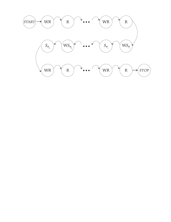
Figure 1: The state diagram of the FSA run by processor $i$. The first row consists of $i$ couples $(W\!R,R)$. $({\mathcal{P}}_{1},\dots,{\mathcal{P}}_{N})$ represents a permutation of the $N$ integers $0,\dots,i-1,i+1,\dots,N$. The last row contains $N-i$ couples $(W\!R,R)$.

Once processor $i$ has successfully received $i$ messages, it gains the right to broadcast, which it does according to the rule expressed in the second row of Fig. 1: it orderly sends its message to its fellows, the $j$-th message being sent to processor ${\mathcal{P}}_{j}$.

The third row of Fig. 1 represents the reception of the remaining $N-i$ messages, coded as $N-i$ couples like those in the first row.

We experimentally observed that, regardless the value of $\mathcal{P}$, such FSA’s represent a distributed algorithm which solves the problem of Definition 2 without deadlocks. As intuition may suggest, the choice of which permutation to use has indeed a deep impact on the overall performance of the algorithm, together with the physical characteristics of the communication line. Reporting on this impact is one of the aims of this paper.

To this end, let us furthermore define:

Definition 7 (run)

The collection of slots needed to fully execute the above algorithm on a given system, together with the value of the corresponding actions.

Definition 8 (average slot utilization)

The average number of slots used during a time step. It represents the average degree of parallelism exploited in the system. It will be indicated as $\mu_{N}$, or simply as $\mu$. It varies between 0 and $N+1$.

Definition 9 (efficiency)

The percentage of used slots over the total number of slots available during a run. $\varepsilon_{N}$, or more simply $\varepsilon$, will be used to represent efficiency.

Definition 10 (length)

The number of time steps in a run. It represents a measure of the time needed by the distributed algorithm to complete. $\lambda_{N}$, or more simply $\lambda$, will be used for lengths.

Definition 11 (number of slots)

$\sigma(N)=(N+1)\lambda_{N}$ represents the number of slots available within a run of $N+1$ processors.

Definition 12 (number of used slots)

For each run and each time step $t$,

$$\nu_{t}=\sum_{i=0}^{N}\delta_{i,t}$$

represents the number of slots that have been used during $t$.

Definition 13 (utilization string)

The $\lambda$-tuple

$$\vec{\nu}=[\nu_{1},\nu_{2},\dots,\nu_{\lambda}],$$

orderly representing the number of used slots for each time step, is called utilization string.

In the next Sections, we introduce and discuss three cases of $\mathcal{P}$. We will show how varying the structure of $\mathcal{P}$ may develop extremely different values of $\mu$, $\varepsilon$, and $\lambda$. This fact, coupled with physical constraints pertaining the communication line and with the number of available independent channels, determines the overall performance of this algorithm.

In the following we assume the availability of a fully connected (crossbar) interconnection [17] that allows any processor to communicate with any other processor in one time step.

3 First Case: Identity Permutation

As a first case, let us assume that the structure of $\mathcal{P}$ be fixed. For instance, let $\mathcal{P}$ be equal to the identity permutation:

$$\binom{0,\dots,i-1,i+1,\dots,N}{0,\dots,i-1,i+1,\dots,N},$$ (2)

i.e., in cycle notation [13], $(0)\dots(i-1)(i+1)\dots(N).$

This means that, once processor $i$ gains the right to broadcast, it will first try to send its message to processor 0 (possibly having to wait for it to become available to receive that message), then it will do the same with processor 1, and so forth up to $N$, obviously skipping itself. This is effectively represented in Table 1 for $N=4$. Let us call this a run-table.

$\stackrel{{\scriptstyle\hbox{\scriptsize id}}}{{\downarrow}}$ $\stackrel{{\scriptstyle\hbox{\scriptsize step}}}{{\rightarrow}}$	1	2	3	4	5	6	7	8	9	10	11	12	13	14	15	16	17	18
0	$S_{1}$	$S_{2}$	$S_{3}$	$S_{4}$	$R_{1}$	$-$	$R_{2}$	$-$	$-$	$-$	$R_{3}$	$-$	$-$	$-$	$R_{4}$	$-$	$-$	$-$
1	$R_{0}$	$\curvearrowright$	$\curvearrowright$	$\curvearrowright$	$S_{0}$	$S_{2}$	$S_{3}$	$S_{4}$	$R_{2}$	$-$	$-$	$R_{3}$	$-$	$-$	$-$	$R_{4}$	$-$	$-$
2	$-$	$R_{0}$	$-$	$-$	$-$	$R_{1}$	$S_{0}$	$\curvearrowright$	$S_{1}$	$S_{3}$	$S_{4}$	$-$	$R_{3}$	$-$	$-$	$-$	$R_{4}$	$-$
3	$-$	$-$	$R_{0}$	$-$	$-$	$-$	$R_{1}$	$-$	$-$	$R_{2}$	$S_{0}$	$S_{1}$	$S_{2}$	$S_{4}$	$-$	$-$	$-$	$R_{4}$
4	$-$	$-$	$-$	$R_{0}$	$-$	$-$	$-$	$R_{1}$	$-$	$-$	$R_{2}$	$-$	$-$	$R_{3}$	$S_{0}$	$S_{1}$	$S_{2}$	$S_{3}$
$\stackrel{{\scriptstyle\hbox{\scriptsize$\vec{\nu}$}}}{{\rightarrow}}$	2	2	2	2	2	2	4	2	2	2	4	2	2	2	2	2	2	2

Table 1: A run ($N=4$), with $\mathcal{P}$ equal to the identity permutation. The step row represents time steps. Id’s identify processors. $\vec{\nu}$ is the utilization string (see Def. 13.) In this case $\mu$, or the average utilization is 2.22 slots out of 5, with an efficiency $\varepsilon=44.44\%$ and a length $\lambda=18$. Note that, if the slot is used, then entry $(i,t)={\mathcal{R}}_{j}$ of this matrix represents relation $i\,{\mathcal{R}}^{t}j$.

It is possible to characterize precisely the duration of the algorithm adopting this permutation:

Proposition 14

$\lambda_{N}=\frac{3}{4}N^{2}+\frac{5}{4}N+\frac{1}{2}{\lfloor{N/2}\rfloor}.$

PROOF (by induction) Let us consider run-table $N+1$. Let us strip off its last row; then wipe out the ${\lfloor{(N+1)/2}\rfloor}-1$ leftmost columns which contain element $S_{N+1}$. Let us also cut out the whole right part of the table starting at the column containing the last occurrence of $S_{N+1}$. Finally, let us rename all the remaining $S_{N+1}$’s as “$-$”.

Our first goal is showing that what remains is run-table $N$. To this end, let us first point out how the only actions that affect the content of other cells in a run-table are the $S$ actions. Their range of action is given by their subscript: an $S_{N+1}$ for instance only affects an entry in row $N+1$.

Now consider what happens when processor $i-1$ sends its message to processor $i$ and this latter gains the right to broadcast as well: at this point, processor $i$ starts sending to processors in the range $\{0,\dots,i-2\}$ i.e., those “above”; as soon as it tries to reach processor $i-1$, in the case this latter has not finished its own broadcast, $i$ enters state $W\!S$ and blocks.

This means that:

1. processors “below” processor $i$ will not be allowed to start their broadcast, and

2. for processor $i$ and those “above”, $\mu$, or the degree of parallelism, is always equal to 2 or 4—no other value is possible. This is shown for instance in Table 1, row “$\vec{\nu}\,$”.

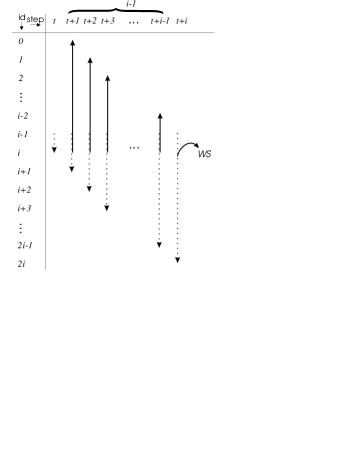
Figure 2: Processor $i-1$ blocks processor $i$ only if $2i-1<N$. A transmission i.e., two used slots, is represented by an arrow. In dotted arrows the sender is processor $i-1$, for normal arrows it is processor $i$. Note the cluster of $i-1$ columns with two concurrent transmissions (adding up to 4 used slots) in each of them.

As depicted in Fig. 2, processor $i$ gets blocked only if it tries to send to processor $i-1$ while this latter is still broadcasting, which happens when $i<\frac{N+1}{2}$—this condition is true for any processor $j\in\{1,\dots,{\lfloor{\frac{N+1}{2}}\rfloor}-1\}$. Note how a “cluster” appears, consisting of $j-1$ columns with 4 used slots inside (Table 2 can be used to verify the above when $N$ is 7.) Removing the first ${\lfloor{\frac{N+1}{2}}\rfloor}$ occurrences of $S_{N+1}$ (from row 0 to row ${\lfloor{\frac{N+1}{2}}\rfloor}-1$) therefore simply shortens of one time step the stay of each processor in their current waiting states. All remnant columns containing that element cannot be removed—these occurrences simply vanish by substituting them with a “$-$” action.

$\stackrel{{\scriptstyle\hbox{\scriptsize id}}}{{\downarrow}}$ $\stackrel{{\scriptstyle\hbox{\scriptsize step}}}{{\rightarrow}}$	1	2	3	4	5	6	7	8	9	10	11	12	13	14	15	16	17	18	19	20	21	22	23	24
0	$S_{1}$	$S_{2}$	$S_{3}$	$S_{4}$	$S_{5}$	$S_{6}$	$S_{7}$	$R_{1}$	$-$	$R_{2}$	$-$	$-$	$-$	$-$	$-$	$-$	$R_{3}$	$-$	$-$	$-$	$-$	$-$	$R_{4}$	$-$
1	$R_{0}$	$\curvearrowright$	$\curvearrowright$	$\curvearrowright$	$\curvearrowright$	$\curvearrowright$	$\curvearrowright$	$S_{0}$	$S_{2}$	$S_{3}$	$S_{4}$	$S_{5}$	$S_{6}$	$S_{7}$	$R_{2}$	$-$	$-$	$R_{3}$	$-$	$-$	$-$	$-$	$-$	$R_{4}$
2	$-$	$R_{0}$	$-$	$-$	$-$	$-$	$-$	$-$	$R_{1}$	$S_{0}$	$\curvearrowright$	$\curvearrowright$	$\curvearrowright$	$\curvearrowright$	$S_{1}$	$S_{3}$	$S_{4}$	$S_{5}$	$S_{6}$	$S_{7}$	$R_{3}$	$-$	$-$	$-$
3	$-$	$-$	$R_{0}$	$-$	$-$	$-$	$-$	$-$	$-$	$R_{1}$	$-$	$-$	$-$	$-$	$-$	$R_{2}$	$S_{0}$	$S_{1}$	$\curvearrowright$	$\curvearrowright$	$S_{2}$	$S_{4}$	$S_{5}$	$S_{6}$
4	$-$	$-$	$-$	$R_{0}$	$-$	$-$	$-$	$-$	$-$	$-$	$R_{1}$	$-$	$-$	$-$	$-$	$-$	$R_{2}$	$-$	$-$	$-$	$-$	$R_{3}$	$S_{0}$	$S_{1}$
5	$-$	$-$	$-$	$-$	$R_{0}$	$-$	$-$	$-$	$-$	$-$	$-$	$R_{1}$	$-$	$-$	$-$	$-$	$-$	$R_{2}$	$-$	$-$	$-$	$-$	$R_{3}$	$-$
6	$-$	$-$	$-$	$-$	$-$	$R_{0}$	$-$	$-$	$-$	$-$	$-$	$-$	$R_{1}$	$-$	$-$	$-$	$-$	$-$	$R_{2}$	$-$	$-$	$-$	$-$	$R_{3}$
7	$-$	$-$	$-$	$-$	$-$	$-$	$R_{0}$	$-$	$-$	$-$	$-$	$-$	$-$	$R_{1}$	$-$	$-$	$-$	$-$	$-$	$R_{2}$	$-$	$-$	$-$	$-$
$\stackrel{{\scriptstyle\hbox{\scriptsize$\vec{\nu}$}}}{{\rightarrow}}$	2	2	2	2	2	2	2	2	2	4	2	2	2	2	2	2	4	4	2	2	2	2	4	4

$\stackrel{{\scriptstyle\hbox{\scriptsize id}}}{{\downarrow}}$ $\stackrel{{\scriptstyle\hbox{\scriptsize step}}}{{\rightarrow}}$	25	26	27	28	29	30	31	32	33	34	35	36	37	38	39	40	41	42	43	44	45	46	47
0	$-$	$-$	$-$	$R_{5}$	$-$	$-$	$-$	$-$	$-$	$R_{6}$	$-$	$-$	$-$	$-$	$-$	$-$	$R_{7}$	$-$	$-$	$-$	$-$	$-$	$-$
1	$-$	$-$	$-$	$-$	$R_{5}$	$-$	$-$	$-$	$-$	$-$	$R_{6}$	$-$	$-$	$-$	$-$	$-$	$-$	$R_{7}$	$-$	$-$	$-$	$-$	$-$
2	$R_{4}$	$-$	$-$	$-$	$-$	$R_{5}$	$-$	$-$	$-$	$-$	$-$	$R_{6}$	$-$	$-$	$-$	$-$	$-$	$-$	$R_{7}$	$-$	$-$	$-$	$-$
3	$S_{7}$	$R_{4}$	$-$	$-$	$-$	$-$	$R_{5}$	$-$	$-$	$-$	$-$	$-$	$R_{6}$	$-$	$-$	$-$	$-$	$-$	$-$	$R_{7}$	$-$	$-$	$-$
4	$S_{2}$	$S_{3}$	$S_{5}$	$S_{6}$	$S_{7}$	$-$	$-$	$R_{5}$	$-$	$-$	$-$	$-$	$-$	$R_{6}$	$-$	$-$	$-$	$-$	$-$	$-$	$R_{7}$	$-$	$-$
5	$-$	$-$	$R_{4}$	$S_{0}$	$S_{1}$	$S_{2}$	$S_{3}$	$S_{4}$	$S_{6}$	$S_{7}$	$-$	$-$	$-$	$-$	$R_{6}$	$-$	$-$	$-$	$-$	$-$	$-$	$R_{7}$	$-$
6	$-$	$-$	$-$	$R_{4}$	$-$	$-$	$-$	$-$	$R_{5}$	$S_{0}$	$S_{1}$	$S_{2}$	$S_{3}$	$S_{4}$	$S_{5}$	$S_{7}$	$-$	$-$	$-$	$-$	$-$	$-$	$R_{7}$
7	$R_{3}$	$-$	$-$	$-$	$R_{4}$	$-$	$-$	$-$	$-$	$R_{5}$	$-$	$-$	$-$	$-$	$-$	$R_{6}$	$S_{0}$	$S_{1}$	$S_{2}$	$S_{3}$	$S_{4}$	$S_{5}$	$S_{6}$
$\stackrel{{\scriptstyle\hbox{\scriptsize$\vec{\nu}$}}}{{\rightarrow}}$	4	2	2	4	4	2	2	2	2	4	2	2	2	2	2	2	2	2	2	2	2	2	2

Table 2: Run-table 7 for $\mathcal{P}$ equal to the identity permutation. Average utilization is 2.38 slots out of 8, or an efficiency of 29.79%.

Finally, the removal of the last occurrence of $S_{N+1}$ from the series of sending actions which constitute the broadcast of processor $N$ allows the removal of the whole right sub-table starting at that point. The obtained table contains all and only the actions of run $N$; the coherence of these action is not affected; and all broadcast sessions are managed according to the rule of the identity permutation. In other words, this is run-table $N$.

Now let us consider $\sigma(N+1)$: according to the above argument, this is equal to:

1. the number of slots available in a $N$-run i.e., $\sigma(N)$,

2. plus $N+1$ slots from each of the columns that witness a delay i.e.,

   $${\lfloor{(N+1)/2}\rfloor}\cdot(N+1),$$

3. plus the slots in the right sub-matrix, not counting the last row i.e.,

   $$(N+1)(N+2),$$

4. plus an additional row.

In other words, $\sigma(N+1)$ can be expressed as the sum of the above first three item multiplied by a factor equal to $\frac{N+2}{N+1}$. This can be written as an equation as

$$\sigma(k+1)=\bigl{(}\sigma(k)+{\lfloor{\frac{k+1}{2}}\rfloor}(k+1)+(k+1)(k+2)\bigr{)}\frac{k+2}{k+1}.$$ (3)

By Definition 11, this brings to the following recursive relation:

$$\lambda(k+1)=\lambda(k)+{\lfloor{\frac{k+1}{2}}\rfloor}+k+2.$$ (4)

Furthermore, the following is true by the induction hypothesis:

$$\lambda_{N}=\lambda(N)=\frac{3}{4}N^{2}+\frac{5}{4}N+\frac{1}{2}{\lfloor{N/2}\rfloor},$$ (5)

Our goal is to show that Eq. (4) and Eq. (5) together imply that $\lambda(N+1)=\lambda_{N+1}$, this latter being

$$\lambda_{N+1} = \frac{3}{4}(N+1)^{2}+\frac{5}{4}(N+1)+\frac{1}{2}{\lfloor{\frac{N+1}{2}}\rfloor}$$ (6)

$$= \frac{3}{4}N^{2}+\frac{11}{4}N+2+\frac{1}{2}{\lfloor{\frac{N+1}{2}}\rfloor}.$$ (7)

Now, let us suppose $N$ is even—this implies that ${\lfloor{(N+1)/2}\rfloor}={\lfloor{N/2}\rfloor}=N/2$. Exploiting this in Eq. (4) for $k=N$ and in Eq. (5), and substituting the latter in the former Equation, brings us to the following result:

$$\lambda(N+1) = \lambda(N)+{\lfloor{\frac{N+1}{2}}\rfloor}+N+2$$

$$= \lambda_{N}+\frac{3}{2}N+2$$

$$= \frac{3}{4}N^{2}+\frac{5}{4}N+\frac{N}{4}+\frac{3}{2}N+2$$

$$= \frac{3}{4}N^{2}+3N+2$$

$$= \frac{3}{4}N^{2}+\frac{11}{4}N+2+\frac{1}{2}{\lfloor{\frac{N+1}{2}}\rfloor},$$

which is equal to $\lambda_{N+1}$ because of Eq. (7). On the other hand, if $N>0$ is odd, then ${\lfloor{(N+1)/2}\rfloor}=(N+1)/2$, while ${\lfloor{N/2}\rfloor}=(N-1)/2$. With the same approach as above we get:

$$\lambda(N+1) = \lambda(N)+{\lfloor{\frac{N+1}{2}}\rfloor}+N+2$$

$$= \frac{3}{4}N^{2}+\frac{5}{4}N+\frac{1}{2}{\lfloor{N/2}\rfloor}+(N+1)/2+N+2$$

$$= \frac{3}{4}N^{2}+\frac{5}{4}N+(N-1)/4+(N+1)/2+N+2$$

$$= \frac{3}{4}N^{2}+\frac{3}{2}N+\frac{3}{4}+\frac{5}{4}N+\frac{5}{4}+(N+1)/4$$

$$= \frac{3}{4}(N+1)^{2}+\frac{5}{4}(N+1)+\frac{1}{2}{\lfloor{\frac{N+1}{2}}\rfloor},$$

which is again equal to $\lambda_{N+1}$ because of Eq. (6). ∎

Lemma 15

The number of columns with 4 used slots inside, for a run with $\mathcal{P}$ equal to the identity permutation and $N+1$ processors, is

$$\sum_{i=0}^{N-1}{\lfloor{\frac{i}{2}}\rfloor}.$$ (8)

[Proof.] Figure 2 shows also how, for any processor $1\leq i\leq{\lfloor{(N+1)/2}\rfloor}$, there exists only one cluster of $i-1$ columns such that each column contains exactly 4 used slots. Moreover Fig. 3 shows that, for any processor ${\lfloor{(N+1)/2}\rfloor}+1\leq i\leq N$, there exists only one cluster of $N-i$ columns with that same property.

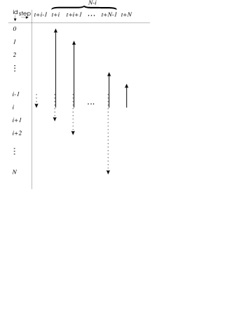
Figure 3: For any processor $i>{\lfloor{(N+1)/2}\rfloor}$, there exists only one cluster of $N-i$ columns with 4 used slots inside.

Let us call $u_{4}$ this number and count such columns:

$$u_{4}=\sum_{i=1}^{{\lfloor{(N+1)/2}\rfloor}}(i-1)+\sum_{i={\lfloor{(N+1)/2}\rfloor}+1}^{N}(N-i).$$ (9)

Via two well-known algebraic transformations on sums (see e.g., in [7, 18]) we get to

$$u_{4}=\sum_{j=0}^{{\lfloor{(N+1)/2}\rfloor}-1}j+\sum_{j=0}^{N-{\lfloor{(N+1)/2}\rfloor}-1}(N-{\lfloor{\frac{N+1}{2}}\rfloor}-1-j).$$ (10)

Now, if $N$ is even, then

$$u_{4} = \sum_{j=0}^{N/2-1}j+\sum_{j=0}^{N/2-1}(\frac{N}{2}-1-j)$$

$$= \sum_{j=0}^{N/2-1}(\frac{N}{2}-1)$$

$$= (\frac{N}{2})(\frac{N}{2}-1)$$

$$= 2\sum_{i=0}^{N/2-1}i$$

$$= \sum_{i=0}^{N-1}{\lfloor{\frac{i}{2}}\rfloor},$$

while, if $N$ is odd,

$$u_{4} = \sum_{j=0}^{(N-1)/2}j+\sum_{j=0}^{(N-3)/2}(\frac{N-3}{2}-j)$$

$$= \frac{N-1}{2}+\sum_{j=0}^{(N-3)/2}\frac{N-3}{2}$$

$$= \frac{N-1}{2}+\frac{N-1}{2}\frac{N-3}{2}$$

$$= \frac{N-1}{2}+2\sum_{i=0}^{(N-3)/2}i$$

$$= \sum_{i=0}^{N-1}{\lfloor{\frac{i}{2}}\rfloor}.$$

∎

Figure 4 shows the typical shape of run-tables in the case of $\mathcal{P}$ being the identity permutation, also locating the 4-used slot clusters.

The following Propositions locate the asymptotic values of $\mu$ and $\varepsilon$:

Proposition 16

$\lim_{k\rightarrow\infty}\varepsilon_{k}=0.$

[Proof.] Let us call $U(k)$ the number of used slots in a run of $k$ processors. As a consequence of Lemma 15, the number of used slots in a run is

$$U(k) = 2\sum_{i=0}^{k-1}{\lfloor{\frac{i}{2}}\rfloor}+2\lambda_{k}$$ (13)

$$= 2\sum_{i=0}^{k-1}{\lfloor{\frac{i}{2}}\rfloor}+2(\frac{3}{4}k^{2}+\frac{5}{4}k+\frac{1}{2}{\lfloor{k/2}\rfloor}).$$

From Definition 11 we derive that

$$\varepsilon_{k}=\frac{U(k)}{(k+1)\lambda_{k}}.$$ (14)

Eq. (3) and Eq. (3) show that $\deg[U(k)]=2$, while from Prop. 14 we know that $\deg[(k+1)\cdot\lambda_{k}]=3$. As a consequence, $\varepsilon_{k}$ tends to zero as $k$ tends to infinity. ∎

Proposition 17

$\lim_{k\rightarrow\infty}\mu_{k}=\frac{8}{3}.$

[Proof.] Being

$$\mu_{k}=\frac{U(k)}{\lambda_{k}},$$ (15)

it is possible to derive that

$$\mu_{k} = \frac{2\frac{k^{2}}{4}+2\frac{3}{4}k^{2}+\hbox{ \emph{ \ldots some 1st degree elements}}}{\frac{3}{4}k^{2}+\hbox{ \emph{ \ldots some 1st degree elements}}}$$ (16)

$$= \frac{2k^{2}+\hbox{ \emph{ \ldots some 1st degree elements}}}{\frac{3}{4}k^{2}+\hbox{ \emph{ \ldots some 1st degree elements}}},$$

which tends to $\frac{8}{3}$, or $2.\overline{6}$, when $k$ goes to infinity. ∎

Figure 4: A graphical representation for run-table 20 when $\mathcal{P}$ is the identity permutation. Light gray pixels represent wasted slots, gray pixels represent $R$ actions, black slots are sending actions. Note the black “blocks” which represent the clusters mentioned in Fig. 2 and Fig. 3.

4 Second Case: Pseudo-random Permutations

This Section covers the case such that $\mathcal{P}$ is a pseudo-random permutation of the integers $0,\dots,i-1,i+1,\dots,N$.

Figure 5 shows the values of $\lambda$ using the identity and random permutations and graphs the parabola who best fits with these latter values. We conclude that, experimentally, the choice of case one is even “worse” than choosing permutations at random. The same conclusion follows from Fig. 6 and Fig. 7 which respectively confront the averages and efficiencies in the above two cases.

Table 3 shows run-table 5, and Fig. 8 shows the shape of run-table 20 in this case.

$\stackrel{{\scriptstyle\hbox{\scriptsize id}}}{{\downarrow}}$ $\stackrel{{\scriptstyle\hbox{\scriptsize step}}}{{\rightarrow}}$	1	2	3	4	5	6	7	8	9	10	11	12	13	14	15	16	17	18	19	20	21	22	23	24
0	$S_{5}$	$S_{1}$	$S_{3}$	$S_{2}$	$S_{4}$	$R_{1}$	$-$	$-$	$-$	$-$	$R_{2}$	$-$	$-$	$-$	$R_{3}$	$-$	$-$	$-$	$-$	$R_{4}$	$R_{5}$	$-$	$-$	$-$
1	$-$	$R_{0}$	$S_{5}$	$\curvearrowright$	$\curvearrowright$	$S_{0}$	$S_{3}$	$S_{2}$	$S_{4}$	$R_{2}$	$-$	$-$	$-$	$R_{3}$	$-$	$-$	$-$	$-$	$R_{4}$	$R_{5}$	$-$	$-$	$-$	$-$
2	$-$	$-$	$-$	$R_{0}$	$-$	$-$	$-$	$R_{1}$	$S_{5}$	$S_{1}$	$S_{0}$	$S_{3}$	$S_{4}$	$-$	$-$	$R_{3}$	$-$	$-$	$-$	$-$	$-$	$R_{4}$	$R_{5}$	$-$
3	$-$	$-$	$R_{0}$	$-$	$-$	$-$	$R_{1}$	$-$	$-$	$-$	$-$	$R_{2}$	$S_{5}$	$S_{1}$	$S_{0}$	$S_{2}$	$S_{4}$	$-$	$-$	$-$	$R_{4}$	$R_{5}$	$-$	$-$
4	$-$	$-$	$-$	$-$	$R_{0}$	$-$	$-$	$-$	$R_{1}$	$-$	$-$	$-$	$R_{2}$	$-$	$-$	$-$	$R_{3}$	$S_{5}$	$S_{1}$	$S_{0}$	$S_{3}$	$S_{2}$	$-$	$R_{5}$
5	$R_{0}$	$-$	$R_{1}$	$-$	$-$	$-$	$-$	$-$	$R_{2}$	$-$	$-$	$-$	$R_{3}$	$-$	$-$	$-$	$-$	$R_{4}$	$\curvearrowright$	$S_{1}$	$S_{0}$	$S_{3}$	$S_{2}$	$S_{4}$
$\stackrel{{\scriptstyle\hbox{\scriptsize$\vec{\nu}$}}}{{\rightarrow}}$	2	2	4	2	2	2	2	2	4	2	2	2	4	2	2	2	2	2	2	4	4	4	2	2

Table 3: Run-table 5 when $\mathcal{P}$ is chosen pseudo-randomly. $\mu$ is $2.5$ slots out of 6, which implies an efficiency of 41.67%.

Figure 5: Comparison between lengths in the case of the identity permutation (dotted parabola) and that of the random permutation (piecewise line), $1\leq N\leq 160$. The lowest curve ($\lambda=0.71N^{2}-3.88N+88.91$) is the parabola best fitting with the piecewise line—which suggests a quadratic execution time as in the case of the identity permutation.

Figure 6: Comparison between values of $\mu$ in the case of a pseudo-random permutation (piecewise line) and that of the identity permutation (dotted curve), $1\leq N\leq 160$. Note how the former is strictly over the latter. Note also how $\mu$ seems to tend to a value right above $2.6$ for the identity permutation, as claimed by Prop. 17.

Figure 7: Comparison between values of $\varepsilon$ in the case of the random permutation (piecewise line) and that of the identity permutation (dotted curve), $1\leq N\leq 160$. Also in this graph the former is strictly over the latter, though they get closer to each other and to zero as $N$ increases, as proven for the identity permutation in Prop. 16.

Figure 8: A graphical representation for run-table 20 when $\mathcal{P}$ is a pseudo-random permutation.

5 Third Case: the Algorithm of Pipelined Broadcast

Let $\mathcal{P}$ be the following permutation:

$$\binom{0,\dots,i-1,i+1,\dots,N}{i+1,\dots,N,0,\dots,i-1}.$$ (17)

Note how permutation (17) is equivalent to $i$ cyclic logical left shifts of the identity permutation. Note also how, in cycle notation [13], (17) is represented as one cycle; for instance,

$$\binom{0,1,2,4,5}{4,5,0,1,2},$$

i.e., (17) for $N=5$ and $i=3$, is equivalent to cycle $(0,4,1,5,2)$.

A value of $\mathcal{P}$ equal to permutation (17) means that, once processor $i$ has gained the right to broadcast, it will first send its message to processor $i+1$ (possibly having to wait for it to become available to receive that message), then it will do the same with processor $i+2$, and so forth up to $N$, then wrapping around and going from processor 0 to processor $i-1$. This is represented in Table 4 for $N=9$.

Pictures quite similar to Table 4 can be found in many classical works on pipelined microprocessors (see e.g. [17, p.132–133].) Indeed, a pipeline is a series of data-paths shifted in time so to overlap their execution, the same way Eq. (17) tends to overlap as much as possible its broadcast sessions. Clearly pipe stages are represented here as full processors, and the concept of machine cycle, or pipe stage time of pipelined processor, simply collapses to the concept of time step as introduced in Def. 3.

A number of considerations like those above brought us to the name we use for this special case of our algorithm, as algorithm of “pipelined gossiping.” We will remark them in the following using the italics typeface.

$\stackrel{{\scriptstyle\hbox{\scriptsize id}}}{{\downarrow}}$ $\stackrel{{\scriptstyle\hbox{\scriptsize step}}}{{\rightarrow}}$	1	2	3	4	5	6	7	8	9	10	11	12	13	14	15	16	17	18	19	20	21	22	23	24	25	26	27
0	$S_{1}$	$S_{2}$	$S_{3}$	$S_{4}$	$S_{5}$	$S_{6}$	$S_{7}$	$S_{8}$	$S_{9}$	$-$	$R_{1}$	$R_{2}$	$R_{3}$	$R_{4}$	$R_{5}$	$R_{6}$	$R_{7}$	$R_{8}$	$R_{9}$	$-$	$-$	$-$	$-$	$-$	$-$	$-$	$-$
1	$R_{0}$	$\curvearrowright$	$S_{2}$	$S_{3}$	$S_{4}$	$S_{5}$	$S_{6}$	$S_{7}$	$S_{8}$	$S_{9}$	$S_{0}$	$-$	$R_{2}$	$R_{3}$	$R_{4}$	$R_{5}$	$R_{6}$	$R_{7}$	$R_{8}$	$R_{9}$	$-$	$-$	$-$	$-$	$-$	$-$	$-$
2	$-$	$R_{0}$	$R_{1}$	$\curvearrowright$	$S_{3}$	$S_{4}$	$S_{5}$	$S_{6}$	$S_{7}$	$S_{8}$	$S_{9}$	$S_{0}$	$S_{1}$	$-$	$R_{3}$	$R_{4}$	$R_{5}$	$R_{6}$	$R_{7}$	$R_{8}$	$R_{9}$	$-$	$-$	$-$	$-$	$-$	$-$
3	$-$	$-$	$R_{0}$	$R_{1}$	$R_{2}$	$\curvearrowright$	$S_{4}$	$S_{5}$	$S_{6}$	$S_{7}$	$S_{8}$	$S_{9}$	$S_{0}$	$S_{1}$	$S_{2}$	$-$	$R_{4}$	$R_{5}$	$R_{6}$	$R_{7}$	$R_{8}$	$R_{9}$	$-$	$-$	$-$	$-$	$-$
4	$-$	$-$	$-$	$R_{0}$	$R_{1}$	$R_{2}$	$R_{3}$	$\curvearrowright$	$S_{5}$	$S_{6}$	$S_{7}$	$S_{8}$	$S_{9}$	$S_{0}$	$S_{1}$	$S_{2}$	$S_{3}$	$-$	$R_{5}$	$R_{6}$	$R_{7}$	$R_{8}$	$R_{9}$	$-$	$-$	$-$	$-$
5	$-$	$-$	$-$	$-$	$R_{0}$	$R_{1}$	$R_{2}$	$R_{3}$	$R_{4}$	$\curvearrowright$	$S_{6}$	$S_{7}$	$S_{8}$	$S_{9}$	$S_{0}$	$S_{1}$	$S_{2}$	$S_{3}$	$S_{4}$	$-$	$R_{6}$	$R_{7}$	$R_{8}$	$R_{9}$	$-$	$-$	$-$
6	$-$	$-$	$-$	$-$	$-$	$R_{0}$	$R_{1}$	$R_{2}$	$R_{3}$	$R_{4}$	$R_{5}$	$\curvearrowright$	$S_{7}$	$S_{8}$	$S_{9}$	$S_{0}$	$S_{1}$	$S_{2}$	$S_{3}$	$S_{4}$	$S_{5}$	$-$	$R_{7}$	$R_{8}$	$R_{9}$	$-$	$-$
7	$-$	$-$	$-$	$-$	$-$	$-$	$R_{0}$	$R_{1}$	$R_{2}$	$R_{3}$	$R_{4}$	$R_{5}$	$R_{6}$	$\curvearrowright$	$S_{8}$	$S_{9}$	$S_{0}$	$S_{1}$	$S_{2}$	$S_{3}$	$S_{4}$	$S_{5}$	$S_{6}$	$-$	$R_{8}$	$R_{9}$	$-$
8	$-$	$-$	$-$	$-$	$-$	$-$	$-$	$R_{0}$	$R_{1}$	$R_{2}$	$R_{3}$	$R_{4}$	$R_{5}$	$R_{6}$	$R_{7}$	$\curvearrowright$	$S_{9}$	$S_{0}$	$S_{1}$	$S_{2}$	$S_{3}$	$S_{4}$	$S_{5}$	$S_{6}$	$S_{7}$	$-$	$R_{9}$
9	$-$	$-$	$-$	$-$	$-$	$-$	$-$	$-$	$R_{0}$	$R_{1}$	$R_{2}$	$R_{3}$	$R_{4}$	$R_{5}$	$R_{6}$	$R_{7}$	$R_{8}$	$\curvearrowright$	$S_{0}$	$S_{1}$	$S_{2}$	$S_{3}$	$S_{4}$	$S_{5}$	$S_{6}$	$S_{7}$	$S_{8}$
$\stackrel{{\scriptstyle\hbox{\scriptsize$\vec{\nu}$}}}{{\rightarrow}}$	2	2	4	4	6	6	8	8	10	8	10	8	10	8	10	8	10	8	10	8	8	6	6	4	4	2	2

Table 4: Run-table of a run for $N=9$ using permutation of Eq. (17). In this case $\mu$, or the average utilization is 6.67 slots out of 10, with an efficiency $\varepsilon=66.67\%$ and a length $\lambda=27$. Note that $\vec{\nu}$ is in this case a palindrome i.e., as well known [24], a string like “21012” which can be read indifferently from left to right or vice-versa.

Clearly using this permutation leads to better performance. In particular, after a start-up phase (after filling the pipeline), sustained performance is close to the maximum—a number of unused slots (pipeline bubbles) still exist, even in the sustained region, but here $\mu$ reaches value $N+1$ half of the times (if $N$ is odd). In the region of decay, starting from time step 19, every new time step a processor fully completes its task. Similar remarks apply to Table 5; this is the typical shape of a run-table for $N$ even. This time the state within the sustained region is more steady, though the maximum number of used slots never reaches the number of slots in the system.

$\stackrel{{\scriptstyle\hbox{\scriptsize id}}}{{\downarrow}}$ $\stackrel{{\scriptstyle\hbox{\scriptsize step}}}{{\rightarrow}}$	1	2	3	4	5	6	7	8	9	10	11	12	13	14	15	16	17	18	19	20	21	22	23	24
0	$S_{1}$	$S_{2}$	$S_{3}$	$S_{4}$	$S_{5}$	$S_{6}$	$S_{7}$	$S_{8}$	$-$	$R_{1}$	$R_{2}$	$R_{3}$	$R_{4}$	$R_{5}$	$R_{6}$	$R_{7}$	$R_{8}$	$-$	$-$	$-$	$-$	$-$	$-$	$-$
1	$R_{0}$	$\curvearrowright$	$S_{2}$	$S_{3}$	$S_{4}$	$S_{5}$	$S_{6}$	$S_{7}$	$S_{8}$	$S_{0}$	$-$	$R_{2}$	$R_{3}$	$R_{4}$	$R_{5}$	$R_{6}$	$R_{7}$	$R_{8}$	$-$	$-$	$-$	$-$	$-$	$-$
2	$-$	$R_{0}$	$R_{1}$	$\curvearrowright$	$S_{3}$	$S_{4}$	$S_{5}$	$S_{6}$	$S_{7}$	$S_{8}$	$S_{0}$	$S_{1}$	$-$	$R_{3}$	$R_{4}$	$R_{5}$	$R_{6}$	$R_{7}$	$R_{8}$	$-$	$-$	$-$	$-$	$-$
3	$-$	$-$	$R_{0}$	$R_{1}$	$R_{2}$	$\curvearrowright$	$S_{4}$	$S_{5}$	$S_{6}$	$S_{7}$	$S_{8}$	$S_{0}$	$S_{1}$	$S_{2}$	$-$	$R_{4}$	$R_{5}$	$R_{6}$	$R_{7}$	$R_{8}$	$-$	$-$	$-$	$-$
4	$-$	$-$	$-$	$R_{0}$	$R_{1}$	$R_{2}$	$R_{3}$	$\curvearrowright$	$S_{5}$	$S_{6}$	$S_{7}$	$S_{8}$	$S_{0}$	$S_{1}$	$S_{2}$	$S_{3}$	$-$	$R_{5}$	$R_{6}$	$R_{7}$	$R_{8}$	$-$	$-$	$-$
5	$-$	$-$	$-$	$-$	$R_{0}$	$R_{1}$	$R_{2}$	$R_{3}$	$R_{4}$	$\curvearrowright$	$S_{6}$	$S_{7}$	$S_{8}$	$S_{0}$	$S_{1}$	$S_{2}$	$S_{3}$	$S_{4}$	$-$	$R_{6}$	$R_{7}$	$R_{8}$	$-$	$-$
6	$-$	$-$	$-$	$-$	$-$	$R_{0}$	$R_{1}$	$R_{2}$	$R_{3}$	$R_{4}$	$R_{5}$	$\curvearrowright$	$S_{7}$	$S_{8}$	$S_{0}$	$S_{1}$	$S_{2}$	$S_{3}$	$S_{4}$	$S_{5}$	$-$	$R_{7}$	$R_{8}$	$-$
7	$-$	$-$	$-$	$-$	$-$	$-$	$R_{0}$	$R_{1}$	$R_{2}$	$R_{3}$	$R_{4}$	$R_{5}$	$R_{6}$	$\curvearrowright$	$S_{8}$	$S_{0}$	$S_{1}$	$S_{2}$	$S_{3}$	$S_{4}$	$S_{5}$	$S_{6}$	$-$	$R_{8}$
8	$-$	$-$	$-$	$-$	$-$	$-$	$-$	$R_{0}$	$R_{1}$	$R_{2}$	$R_{3}$	$R_{4}$	$R_{5}$	$R_{6}$	$R_{7}$	$\curvearrowright$	$S_{0}$	$S_{1}$	$S_{2}$	$S_{3}$	$S_{4}$	$S_{5}$	$S_{6}$	$S_{7}$
$\stackrel{{\scriptstyle\hbox{\scriptsize$\vec{\nu}$}}}{{\rightarrow}}$	2	2	4	4	6	6	8	8	8	8	8	8	8	8	8	8	8	8	6	6	4	4	2	2

Table 5: Run-table of a run for $N=8$ using the permutation of Eq. (17). $\mu$ is equal to 6 slots out of 9, with an efficiency $\varepsilon=66.67\%$ and a length $\lambda=24$. Note how $\vec{\nu}$ is a palindrome string.

Figure 9: Comparison between run lengths resulting from the identity permutation (dotted parabola) and those from permutation (17). The former are shown for $1\leq N\leq 160$, the latter for $1\leq N\leq 500$.

Figure 10: Comparison between values of $\mu$ derived from the identity permutation (dotted parabola) and those from permutation (17) for $1\leq N\leq 10$.

Figure 11: Comparison of efficiencies when $\mathcal{P}$ is the identity permutation and in the case of permutation (17), for $1\leq N\leq 160$.

It is possible to show that the distributed algorithm described in Fig. 1, with $\mathcal{P}$ as in Eq. (17), can be computed in linear time:

Proposition 18

$$\lambda_{N}=3N.$$

[Proof.]

Let us consider run-table $N+1$. Let us strip off its last row; then remove each occurrence of $S_{N+1}$, shifting each row leftwards of one position. Remove also each occurrence of $R_{N+1}$. Finally, remove the last column, now empty because of the previous rules.

Our first goal is showing that what remains is run-table $N$. To this end, let us remind the reader that each occurrence of an $S_{N+1}$ action only affects row $N+1$, which has been cut out. Furthermore, each occurrence of $R_{N+1}$ comes from an $S$ action in row $N+1$. Finally, due to the structure of the permutation, the last action in row $N+1$ has to be an $S_{N}$—as a consequence, row $N$ shall contain an $R_{N+1}$, and remnant rows shall contain action “$-$”. Removing the $R_{N+1}$ allows to remove the last column as well, with no coherency violation and no redundant steps. This proves our first claim.

With a reasoning similar to the one followed for Prop. 14 we have that

$$\sigma(k+1)=\bigl{(}\sigma(k)+3(k+1)\bigr{)}\frac{k+2}{k+1}.$$ (18)

that is, by Definition 11,

$$\lambda(k+1)=\lambda(k)+3.$$ (19)

Recursive relation (19) represents the first (or forward) difference of $\lambda(k)$ (see e.g., [16]). The solution of the above is $\lambda(k)=3k$.∎

The efficiency of the algorithm of pipelined gossiping does not depend on $N$:

Proposition 19

$\forall k>0:\varepsilon_{k}=2/3$.

[Proof.] Again, let $U(k)$ be the number of used slots in a run of $k$ processors. From Prop. 18 we know that run-table $k$ differs from run-table $k+1$ only for $k+1$ “$S$” actions, $k+1$ “$R$” actions, and the last row consisting of another $k+1$ pairs of useful actions plus some non-useful actions. We conclude that

$$U(k+1)=U(k)+4(k+1).$$ (20)

Via e.g., the method of trial solutions for constant coefficient difference equations introduced in [16, p. 16], we get to $U(k)=2k(k+1)$ which obviously satisfies recursive relation (20) being $2k(k+1)+4(k+1)=2(k+1)(k+2)$.

So

$$\varepsilon_{k}=\frac{U(k)}{\sigma(k)}=\frac{2k(k+1)}{\lambda_{k}(k+1)}=\frac{2}{3}.$$ (21)

∎

Proposition 20

$\forall k>0:\mu_{k}=\frac{2}{3}(k+1)$.

[Proof.] The proof follows immediately from

$$\mu_{k}=U(k)/\lambda_{k}=2k(k+1)/(3k).$$

∎

Table 6 shows how a run-table looks like when multiple gossiping sessions take place one after the other. As a result, the central area corresponding to the best observable performance is prolonged. In such an area, $\varepsilon$ has been experimentally found to be equal to $N/(N+1)$ and the throughput, or the number of fully completed gossipings per time step, has been found to be equal to $t/2$, $t$ being the duration of a time step. In other words, within that area a gossiping is fully completed every two time steps in the average. A number of algorithms which are based on multiple gossipings may greatly benefit from this approach, e.g., those implemented in the distributed voting algorithm described in [3].

	1	2	3	4	5	6	7	8	9	10	11	12	13	14	15	16	17	18	19	$\dots$
0	$S_{1}$	$S_{2}$	$S_{3}$	$S_{4}$	$-$	$R_{1}$	$R_{2}$	$R_{3}$	$R_{4}$	$\curvearrowright$	$S_{1}$	$S_{2}$	$S_{3}$	$S_{4}$	$-$	$R_{1}$	$R_{2}$	$R_{3}$	$R_{4}$	$\dots$	$\curvearrowright$	$S_{1}$	$S_{2}$	$S_{3}$	$S_{4}$	$-$	$R_{1}$	$R_{2}$	$R_{3}$	$R_{4}$	$-$	$-$	$-$
1	$R_{0}$	$\curvearrowright$	$S_{2}$	$S_{3}$	$S_{4}$	$S_{0}$	$-$	$R_{2}$	$R_{3}$	$R_{4}$	$R_{0}$	$\curvearrowright$	$S_{2}$	$S_{3}$	$S_{4}$	$S_{0}$	$-$	$R_{2}$	$R_{3}$	$\dots$	$R_{4}$	$R_{0}$	$\curvearrowright$	$S_{2}$	$S_{3}$	$S_{4}$	$S_{0}$	$-$	$R_{2}$	$R_{3}$	$R_{4}$	$-$	$-$
2	$-$	$R_{0}$	$R_{1}$	$\curvearrowright$	$S_{3}$	$S_{4}$	$S_{0}$	$S_{1}$	$-$	$R_{3}$	$R_{4}$	$R_{0}$	$R_{1}$	$\curvearrowright$	$S_{3}$	$S_{4}$	$S_{0}$	$S_{1}$	$-$	$\dots$	$R_{3}$	$R_{4}$	$R_{0}$	$R_{1}$	$\curvearrowright$	$S_{3}$	$S_{4}$	$S_{0}$	$S_{1}$	$-$	$R_{3}$	$R_{4}$	$-$
3	$-$	$-$	$R_{0}$	$R_{1}$	$R_{2}$	$\curvearrowright$	$S_{4}$	$S_{0}$	$S_{1}$	$S_{2}$	$-$	$R_{4}$	$R_{0}$	$R_{1}$	$R_{2}$	$\curvearrowright$	$S_{4}$	$S_{0}$	$S_{1}$	$\dots$	$S_{2}$	$-$	$R_{4}$	$R_{0}$	$R_{1}$	$R_{2}$	$\curvearrowright$	$S_{4}$	$S_{0}$	$S_{1}$	$S_{2}$	$-$	$R_{4}$
4	$-$	$-$	$-$	$R_{0}$	$R_{1}$	$R_{2}$	$R_{3}$	$\curvearrowright$	$S_{0}$	$S_{1}$	$S_{2}$	$S_{3}$	$-$	$R_{0}$	$R_{1}$	$R_{2}$	$R_{3}$	$\curvearrowright$	$S_{0}$	$\dots$	$S_{1}$	$S_{2}$	$S_{3}$	$-$	$R_{0}$	$R_{1}$	$R_{2}$	$R_{3}$	$\curvearrowright$	$S_{0}$	$S_{1}$	$S_{2}$	$S_{3}$
	2	2	4	4	4	4	4	4	4	4	4	4	4	4	4	4	4	4	4	$\dots$	4	4	4	4	4	4	4	4	4	4	4	2	2

Table 6: The algorithm is modified so that multiple gossiping sessions take place. The central, best performing area is consequently prolonged. Therein $\varepsilon$ is equal to $N/(N+1)$. Note how within that area there are consecutive “zones” of ten columns each, within whom five gossiping sessions reach their conclusion. For instance, such a zone is the region between columns 7 and 16: therein, at entries $(4,7)$, $(0,9)$, $(1,10)$, $(2,11)$, and $(3,12)$, a processor gets the last value of a broadcast and can perform some work on a full set of values. This brings to a throughput of $t/2$, where $t$ is the duration of a slot.

Obviously our model reaches such a performance only if the system calls for exactly one time step to communicate between any two processors, like e.g. in a crossbar system. This is similar to the constraint of hardware pipelined processors which call for a number of memory ports equal to $n$, $n$ being the number of pipeline stages supported by that machine—in this way the system is able to overlap any two of its stages. This of course turns into requiring to have a memory system capable of delivering $n$ times the original bandwidth of a corresponding, unpipelined machine [17].

Figure 12: A graphical representation for run-table 30 when $\mathcal{P}$ is permutation (17).

Note how the specularity of graphs like the one of Fig. 12 translates into a palindrome $\vec{\nu}$ string.

6 Further Optimizations

Evidently the execution of “$-$” and “$\curvearrowright$” actions—the “bubbles”—is an impairment towards the optimum. As a consequence, a general strategy to increase the performance of our algorithms could be the following one:

1. execute a base rule (corresponding to the adoption of any permutation $\mathcal{P}$, like e.g., those presented in §3, §4, or §5), and

2. as soon as there is a wait-in-sending, choose a different destination between those that would execute a wait-in-receiving.

In other words, the processor who gains the right to broadcast does follow the order given by $\mathcal{P}$ unless it knows (by calculating its own run-table) that doing that it would trigger a wait-to-send action. In such latter case, it looks for another candidate among those following the current one in permutation $\mathcal{P}$. If there exists at least one such processor that would otherwise be wasting its slot in a wait-in-receiving, then the message is sent to it. In some sense, this allows each broadcasting processor to rearrange its leading $\mathcal{P}$ into a “better” $\mathcal{P}^{\prime}$, driven by the possibility to (locally) increase the number of used slots. Of course this local gain might turn into a loss later on. In this Section we describe how the above procedure perturbs the values of $\lambda$, $\mu$, and $\varepsilon$ for the so far discussed three cases.

This strategy depicts similarities with the optimization method known as Pipeline Scheduling and described in [17]: for any program $p$ whose run corresponds to the execution of $\mathrm{IC}(p)$ instructions ($\mathrm{IC}(p)$ = instruction count of program $p$), namely

$$(I_{k})_{1\leq k\leq\mathrm{IC}(p)},$$ (22)

the detection of an obstacle to the optimum (a stall) triggers an attempt to go round it by trying to rearrange (22) as

$$(I^{\prime}_{j})_{1\leq j\leq\mathrm{IC}(p)},$$ (23)

where (23) is substantially a (semantically equivalent) permutation of (22) such that the obstacle is removed.

Of course in our case semantical equivalence is guaranteed by the fact that each processor just modifies its permutation on-the-fly. This does not affect the output of the algorithm, so our task is much easier than if we had to implement actual pipeline scheduling.

The following algorithm can be used to simulate a run and compute the entire broadcasting sequence i.e., the second row of Fig. 1:

Algorithm 2

: Gossiping with permutation scheduling

	Input: $N$, $\mathcal{P}$, $p$ (processor id)
	Input: $\mathrm{run}$ (running run-table), $t$ (current time step)
	Input: $m$ (message to be broadcast)
	Output: $\mathrm{run}$, $t$
1	begin
2		$\vec{f}:=\mathrm{TRUE}$					{ set each entry of $\vec{f}$ to $\mathrm{TRUE}$ }
3		$i:=1$
4		$w:=0$
5		while $i\leq N$ do					{ for each symbol of $\mathcal{P}$ }
6			$j:=i+t+w-1$
			{ if $\mathcal{P}_{i}$ has never been used and processor $i$ is available }
7			if $f_{i}=\mathrm{TRUE}\ \wedge\ \mathrm{run}(\mathcal{P}_{i},j)=\mathrm{FREE}$ then
8				$f_{i}:=\mathrm{FALSE}$			{ mark $\mathcal{P}_{i}$ as used }
9				Send $m$ to processor $\mathcal{P}_{i}$
10				$\mathrm{run}(p,j):=p\,S^{j}\,\mathcal{P}_{i}$
11				$\mathrm{run}(\mathcal{P}_{i},j):=\mathcal{P}_{i}\,R^{j}\,p$
12				$i:=i+1$			{ go to next item of $\mathcal{P}$ }
			{ if $\mathcal{P}_{i}$ has been already used or processor $i$ is not available }
13			else				{ i.e., when $f_{i}=\mathrm{FALSE}\ \vee\ \mathrm{run}(\mathcal{P}_{i},j)\neq\mathrm{FREE}$ }
				{ orderly search for a possible substitute }
14				$\mathrm{stop}:=\mathrm{FALSE}$
15				$l:=1$
16				while $l\leq N\ \wedge\ \mathrm{stop}=\mathrm{FALSE}$ do
17					if $f_{l}=\mathrm{TRUE}\ \wedge\ \mathrm{run}(\mathcal{P}_{l},j)=\mathrm{FREE}$ then
18						$\mathrm{stop}:=\mathrm{TRUE}$
19					else
20						$l:=l+1$
21					endif
22				enddo
				{ if a candidate has been found at entry $l$, use $\mathcal{P}_{l}$ instead of $\mathcal{P}_{i}$ }
23				if $\mathrm{stop}=\mathrm{TRUE}$ then
24					$f_{l}:=\mathrm{FALSE}$
25					Send $m$ to processor $\mathcal{P}_{l}$
26					$\mathrm{run}(p,j):=p\,S^{j}\,\mathcal{P}_{l}$
27					$\mathrm{run}(\mathcal{P}_{l},j):=\mathcal{P}_{l}\,R^{j}\,p$
28					$i:=i+1$
29				else			{ if no such an $l$ exists…}
30					$\mathrm{run}(p,j):=\ \curvearrowright$		{ store a wait-for-sending }
					{ deal again with the current value of $i$, but on next column }
31					$w:=w+1$
32				endif
33			endif
34		enddo
35		$t:=t+N+w$
36	end.

6.1 Applying Algorithm 2 to the Case of the Identity Permutation

Figures 13, 14, and 15 describe the improvement we observed by applying optimizing Algorithm 2 to the case of the identity permutation.

Figure 13: This picture portrays and compares run lengths for $1\leq N\leq 160$ when $\mathcal{P}$ is the identity permutation (dotted parabola), when Algorithm 2 is applied to the case of the identity permutation (piecewise line), and in the case of the pipelined gossiping. Note how Algorithm 2 always improves its base method, and in a small number of cases ($N=2^{i}-1,i\leq 10$) it reaches a better performance than that of pipelined gossiping (see Table 8). This is also shown in Fig. 15.

Figure 14: Values of $\mu$ for the three cases of Fig. 13.

We experimentally found that the strategy does greatly improve the values of $\mu$, $\lambda$, and $\varepsilon$. We also observed that a particularly good case occurs when the number of processors employed is a power of two. Table 7 for instance shows run-table 7, that has an efficiency of $73.68\%$. This efficiency though tends to decrease. In particular we found that, after the case of $N=2^{10}-1$, the efficiency becomes lower than $2/3$ i.e., the one of the algorithm of pipelined gossiping (see Table 8.)

$\stackrel{{\scriptstyle\hbox{\scriptsize id}}}{{\downarrow}}$ $\stackrel{{\scriptstyle\hbox{\scriptsize step}}}{{\rightarrow}}$	1	2	3	4	5	6	7	8	9	10	11	12	13	14	15	16	17	18	19
0	$S_{1}$	$S_{2}$	$S_{3}$	$S_{4}$	$S_{5}$	$S_{6}$	$S_{7}$	$R_{1}$	$R_{2}$	$R_{3}$	$R_{4}$	$R_{6}$	$R_{5}$	$R_{7}$	$-$	$-$	$-$	$-$	$-$
1	$R_{0}$	$S_{3}$	$S_{2}$	$S_{5}$	$S_{4}$	$S_{7}$	$S_{6}$	$S_{0}$	$R_{3}$	$R_{2}$	$R_{5}$	$R_{4}$	$R_{6}$	$-$	$R_{7}$	$-$	$-$	$-$	$-$
2	$-$	$R_{0}$	$R_{1}$	$S_{3}$	$S_{6}$	$S_{4}$	$S_{5}$	$S_{7}$	$S_{0}$	$S_{1}$	$R_{3}$	$R_{7}$	$R_{4}$	$R_{5}$	$-$	$-$	$-$	$R_{6}$	$-$
3	$-$	$R_{1}$	$R_{0}$	$R_{2}$	$S_{7}$	$S_{5}$	$S_{4}$	$S_{6}$	$S_{1}$	$S_{0}$	$S_{2}$	$R_{5}$	$R_{7}$	$R_{4}$	$R_{6}$	$-$	$-$	$-$	$-$
4	$-$	$-$	$-$	$R_{0}$	$R_{1}$	$R_{2}$	$R_{3}$	$S_{5}$	$S_{6}$	$S_{7}$	$S_{0}$	$S_{1}$	$S_{2}$	$S_{3}$	$R_{5}$	$R_{6}$	$R_{7}$	$-$	$-$
5	$-$	$-$	$-$	$R_{1}$	$R_{0}$	$R_{3}$	$R_{2}$	$R_{4}$	$S_{7}$	$S_{6}$	$S_{1}$	$S_{3}$	$S_{0}$	$S_{2}$	$S_{4}$	$R_{7}$	$R_{6}$	$-$	$-$
6	$-$	$-$	$-$	$-$	$R_{2}$	$R_{0}$	$R_{1}$	$R_{3}$	$R_{4}$	$R_{5}$	$S_{7}$	$S_{0}$	$S_{1}$	$\curvearrowright$	$S_{3}$	$S_{4}$	$S_{5}$	$S_{2}$	$R_{7}$
7	$-$	$-$	$-$	$-$	$R_{3}$	$R_{1}$	$R_{0}$	$R_{2}$	$R_{5}$	$R_{4}$	$R_{6}$	$S_{2}$	$S_{3}$	$S_{0}$	$S_{1}$	$S_{5}$	$S_{4}$	$\curvearrowright$	$S_{6}$
$\stackrel{{\scriptstyle\hbox{\scriptsize$\vec{\nu}$}}}{{\rightarrow}}$	2	4	4	6	8	8	8	8	8	8	8	8	8	6	6	4	4	2	2

Table 7: Run-table 7 for $\mathcal{P}$ equal to the identity permutation, modified by Algorithm 2 ($\mu=5.89$, $\varepsilon=73.68\%$).

Figure 15: Values of $\varepsilon$ for the three cases of Fig. 13. Peek values are in Table 8.

$i$	1	2	3	4	5	6	7	8	9	10	11
$\varepsilon$	100	85.71	73.68	71.43	69.66	68.11	67.55	67.11	66.88	66.75	65.34

Table 8: $\varepsilon$ values for different values of $N=2^{i}-1$.

6.2 Applying Algorithm 2 to the Case of the Pseudo-Random Permutation

Also when applied to the case of the pseudo-random permutation, Algorithm 2 improves performance—this is shown for $1\leq N\leq 160$ in the Fig. 16, Fig. 17, and Fig. 18. This time the improvement is not as high as in §6.1.

Figure 16: Comparison of lengths when $\mathcal{P}$ is a pseudo-random permutation (dots) and with the addition of Algorithm 2 (piecewise line), $1\leq N\leq 160$.

Figure 17: Comparison of the values of $\mu$ in the two cases of Fig. 16.

Figure 18: Comparison of the values of $\varepsilon$ in the two cases of Fig. 16.

6.3 Applying Algorithm 2 in the Pipelined Broadcast Mode.

When coupling Algorithm 2 to the algorithm of pipelined gossiping, the local optimizations gave unstable, and in some cases even negative returns (see Fig. 19, 20, and 21). For instance, Table 9 is run-table 4, which shows the same values of $\mu$ and $\varepsilon$ as if we had performed no optimization at all. $N=18$ is an example of negative return—in this case e.g., $\varepsilon$ falls to 60%.

$\stackrel{{\scriptstyle\hbox{\scriptsize id}}}{{\downarrow}}$ $\stackrel{{\scriptstyle\hbox{\scriptsize step}}}{{\rightarrow}}$	1	2	3	4	5	6	7	8	9	10	11	12
0	$S_{1}$	$S_{2}$	$S_{3}$	$S_{4}$	$R_{2}$	$R_{1}$	$-$	$R_{3}$	$R_{4}$	$-$	$-$	$-$
1	$R_{0}$	$S_{3}$	$S_{2}$	$\curvearrowright$	$S_{4}$	$S_{0}$	$R_{2}$	$R_{4}$	$R_{3}$	$-$	$-$	$-$
2	$-$	$R_{0}$	$R_{1}$	$S_{3}$	$S_{0}$	$S_{4}$	$S_{1}$	$-$	$-$	$R_{3}$	$R_{4}$	$-$
3	$-$	$R_{1}$	$R_{0}$	$R_{2}$	$\curvearrowright$	$\curvearrowright$	$S_{4}$	$S_{0}$	$S_{1}$	$S_{2}$	$-$	$R_{4}$
4	$-$	$-$	$-$	$R_{0}$	$R_{1}$	$R_{2}$	$R_{3}$	$S_{1}$	$S_{0}$	$\curvearrowright$	$S_{2}$	$S_{3}$
$\stackrel{{\scriptstyle\hbox{\scriptsize$\vec{\nu}$}}}{{\rightarrow}}$	2	4	4	4	4	4	4	4	4	2	2	2

Table 9: Run-table 4 in pipelined gossiping mode and applying Algorithm 2. $\mu=3.33$ slots out of 5, or an efficiency of 66.67%. In other words, Algorithm 2 affected the run-table without developing any improvement—in particular, the ending order has changed.

Figure 19: Values of $\lambda$ for $1\leq N\leq 40$ when $\mathcal{P}$ is (17), with (piecewise line) and without (dotted line) the optimization of Algorithm 2.

Figure 20: Values of $\mu$ in the two cases of Fig. 19.

Figure 21: Values of $\varepsilon$ in the two cases of Fig. 19.

7 Applicative Examples

In this section we provide two example applications for the algorithms described in this paper: a restoring organ (Sect. 7.1) and a proposal for a Hopfield neural network architecture (Sect. 7.2).

7.1 The EFTOS Voting Farm

The EFTOS Voting Farm (VF) is a software component that can be used to implement restoring organs i.e., $N$-modular redundancy systems ($N$MR) with $N$-replicated voters [12] (see Fig. 22). Basic design goals of such tools include fault transparency but also replication transparency, a high degree of flexibility and ease-of-use, and good performance. Restoring organs allow to overcome the shortcoming of having one voter, the failure of which leads to the failure of the whole system even when each and every other module is still running correctly. From the point of view of software engineering, such systems though are characterised by two major drawbacks:

• Each module in the $N$MR must be aware of and responsible for interacting with the whole set of voters;

• The complexity of these interactions, which is a function that increases quadratically with $N$ (the cardinality of the set of voters), burdens each module in the $N$MR.

To overcome these drawbacks, VF adopts a different procedure, as described in Fig. 23: in this new procedure, each module only has to interact with, and be aware of one voter, regardless of the value of $N$.

The VF is an example of an application taking advantage of the algorithms described in this paper: indeed its voters play the role of the processors of Sect. 2. In a fully connected and synchronous system then steady state performance of the VF follows the ones shown in this paper. In particular this leads to high scalability and performance.

A thorough description of the VF can be found in [3].

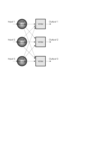
Figure 22: A restoring organ [12], i.e., a $N$-modular redundant system with $N$ voters, when $N=3$. Note that a de-multiplexer is required to produce the single final output.

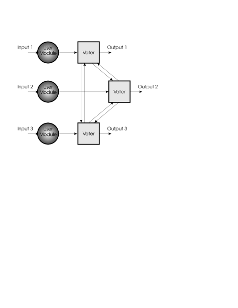
Figure 23: Structure of the EFTOS VF for $N=3$.

7.2 Applications to Hopfield Neural Networks

A well known paradigm of Neural Computing is minimisation [21]. Such cognitive technique has been proved to be able to provide satisfactory solutions to two classes of problems:

1. Recognition, where a partial or corrupted pattern is given as input and the action of the system network is to recognise it as one of its stored patterns.

2. Discovery of local minima—a typical example being the travelling salesman problem [10].

Hopfield networks [9, 19] have been found to be particularly useful in solving the above two classes of problems. A Hopfield network substantially is a net of binary threshold logic units, connected in an all-to-all pattern, with weighted connections between units. Weights are changed according to the so-called Hebb rule—that takes over the role of the training step of, e.g., the multi-layer perceptron [20]. Given a partial or corrupted input pattern, a Hopfield network allows to determine which of the data stored in the network resemble the most the input pattern. This is achieved by means of an iterative procedure, the starting point of which is the input pattern, which consists of serial, element by element updating. This procedure is indeed a gossiping algorithm. When the number of neurons is large the adoption of a scalable procedure like the algorithm of pipelined gossiping could provide a satisfactory solution.

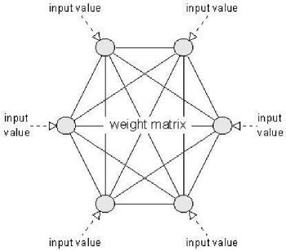
Figure 24: A Hopfield Neural Network.

8 Conclusions and Future Work

As e.g., in [2], a formal model for a family of algorithms depending on a combinatorial parameter, $\mathcal{P}$, has been introduced and discussed. Several case studies have been designed, simulated, and analyzed, also categorizing in some cases their asymptotic bahaviour. In one of these cases—the algorithm of pipelined gossiping—it has been proved that the efficiency of the algorithm does not depend on $N$—a result that overcomes those of all the known gossiping algorithms [14, 11]. An optimizing algorithm has been presented and discussed as well.

We experimentally found that the efficiencies of the base cases, improved via the optimization algorithm, lay in general quite “close” to the efficiency of the algorithm of pipelined gossiping. In particular we found that:

• The simplest base case, leading to the worst observed performance, is the case which best matches the optimizing algorithm 2. Combining this worst case with the optimization actually leads to a great improvement which, for some values of $N$, raises performance even above the values of the “best” base case.

• Nearly no improvement comes when trying to optimize the “best” case.

The two above observations seem to suggest that, from a certain value of $N$ onward, the algorithm of pipelined gossiping actually is the “best” member of the family exposed herein. This is suggested for instance from Fig. 15 and Table 8 which show how even in the best cases, corresponding to a number of processors equals to a power of 2, there is experimental evidence that, sooner or later, the complexity of the problem brings efficiency below 2/3, the one of pipelined gossiping. Fig. 15 shows also that the optimization of the best case in general does not improve the best case without optimization. This brought us to the following Conjecture:

Sooner or later, efficiency reaches a value less than or equal to the one of pipelined gossiping:

Conjecture 21

For any $f$ (function transforming parameters like $\mathcal{P}$), let us call $\varepsilon_{f,k}$ the efficiency of $f$ in a run with $N=k$ and $\varepsilon_{\textsc{pb}}=2/3$ the efficiency of the algorithm of pipelined gossiping; then there exists an integer $m$ such that $\forall n>m:\varepsilon_{f,n}\leq\varepsilon_{\textsc{pb}}.$

Investigating the above Conjecture will be part of future works.

Of course the optimizing Algorithm 2 is not the only one nor the best possible one. On the contrary, it is characterized by an optimization policy which only takes into account the local gain of the current processor, without any reference to possible global optimization strategies (e.g., considering also the scenarios that the rest of the processors are going to face because of the current local choice). Techniques based on trying alternative solutions and choosing the best one, possibly considering future consequences of current, local decisions, may reveal themselves as more appropriate and performant and may be used to validate the considerations that brought us to Conjecture 21.

This paper introduced a family of algorithms depending on a combinatorial parameter and showed that an optimum exists for its performance is a special case—fully connected and synchronous systems. Note how such an optimum may exist also in other cases—an open question that may be dealt with in future work. Should such optima exist, then any tool using our algorithms could adapt to a change in the communication infrastructure by simply “loading” the new optimum. This may have positive relapses on optimal porting of gossiping services or in mobile systems using gossiping.

References

- [1] J.-C. Bermond, L. Gargano, A. A. Rescigno, and U. Vaccaro. Fast gossiping by short messages. SIAM J. Comput., 27:917–941, 1998.
- [2] V. De Florio. The HeartQuake dynamic system. Complex Systems, 9(2):91–114, April 1995.
- [3] V. De Florio, G. Deconinck, and R. Lauwereins. Software tool combining fault masking with user-defined recovery strategies. IEE Proceedings – Software, 145(6):203–211, December 1998. Special Issue on Dependable Computing Systems. IEE in association with the British Computer Society.
- [4] V. De Florio, G. Deconinck, and R. Lauwereins. A novel distributed algorithm for high-throughput and scalable gossiping. In Proc. of the 8th International Conference on High Performance Computing and Networking Europe (HPCN Europe 2000), Lecture Notes in Computer Science, volume 1823, pages 313–322, Amsterdam, The Nederlands, May 2000. Springer-Verlag, Berlin.
- [5] T. F. Gonzales. An efficient algorithm for gossiping in the multicasting communication environment. IEEE Transactions on Parallel and Distributed Systems, 14(7), July 2003.
- [6] I. Graham. The Transputer Handbook. Prentice-Hall, London, 1990.
- [7] D. H. Green and D. E. Knuth. Mathematics for the Analysis of Algorithms. Birkhauser, Boston, MA, 2nd edition, 1986.
- [8] S. Hedetniemi, S. Hedetniemi, and A. Leistman. A survey of gossiping and broadcasting in communication networks. Networks, 18:419–435, 1988.
- [9] J. J. Hopfield. Neural networks and physical systems with emergent collective computational properties. Proc. Nat. Acad. Sci. USA, 79:2554–2558, 1982.
- [10] J. J. Hopfield and D. W. Tank. Neural computation of decisions in optimisation problems. Biol. Cybern., 52:141–152, 1985.
- [11] J. Hromkovic, R. Klasing, B. Monien, and R. Peine. Combinatorial Network Theory, chapter Dissemination of Information in Interconnection Networks (Broadcasting & Gossiping), pages 125–212. Kluwer Academic Publishers, The Netherlands, 1996.
- [12] B. W. Johnson. Design and Analysis of Fault-Tolerant Digital Systems. Addison-Wesley, New York, 1989.
- [13] D. E. Knuth. The Art of Computer Programming, Volume 1 (Fundamental Algorithms). Addison-Wesley, Reading MA, 2nd edition, 1973.
- [14] D. W. Krumme, G. Cybenko, and K. N. Venkataraman. Gossiping in minimal time. SIAM Journal on Computing, 21(1):111–139, 1992.
- [15] L. Lamport, R. Shostak, and M. Pease. The Byzantine generals problem. ACM Trans. on Programming Languages and Systems, 4(3):384–401, July 1982.
- [16] E. S. Page and L. B. Wilson. An Introduction to Computational Combinatorics. Cambridge University Press, Cambridge, 1979.
- [17] D. A. Patterson and J. L. Hennessy. Computer Architecture—A Quantitative Approach. Morgan Kaufmann, S. Francisco, CA, 2nd edition, 1996.
- [18] P. W. Purdon jr. and C. A. Brown. The Analysis of Algorithms. Holt Rinehart and Winston, New York, 1985.
- [19] R. Rojas. Neural Networks — A Systematic Introduction. Springer, 1996.
- [20] F. Rosenblatt. The perceptron: A probabilistic model for information storage and retrieval in the brain. Psych. Rev., 65:386–408, 1958.
- [21] D. Sima, T. Fountain, and P. Kacsuk. Advanced Computer Architectures — A Design-Space Approach. Addison-Wesley, 1997.
- [22] Sun. SunOS 5.5.1 Man Pages. Sun Microsystems, 1994.
- [23] A. S. Tanenbaum. Computer Networks. Prentice-Hall, London, 3rd edition, 1996.
- [24] V. Y. Vilenkin. Combinatorics. Academic Press, New York, 1971.