Distributed Stochastic Market Clearing with
High-Penetration Wind Power

Abstract

Integrating renewable energy into the modern power grid requires risk-cognizant dispatch of resources to account for the stochastic availability of renewables. Toward this goal, day-ahead stochastic market clearing with high-penetration wind energy is pursued in this paper based on the DC optimal power flow (OPF). The objective is to minimize the social cost which consists of conventional generation costs, end-user disutility, as well as a risk measure of the system re-dispatching cost. Capitalizing on the conditional value-at-risk (CVaR), the novel model is able to mitigate the potentially high risk of the recourse actions to compensate wind forecast errors. The resulting convex optimization task is tackled via a distribution-free sample average based approximation to bypass the prohibitively complex high-dimensional integration. Furthermore, to cope with possibly large-scale dispatchable loads, a fast distributed solver is developed with guaranteed convergence using the alternating direction method of multipliers (ADMM). Numerical results tested on a modified benchmark system are reported to corroborate the merits of the novel framework and proposed approaches.

Nomenclature

-A Indices, numbers, and sets

$T$, $\mathcal{T}$

Number and set of scheduling periods.

$N_{b}$, $N_{l}$

Number of buses and lines.

$N_{g}$, $\mathcal{N}_{g}$

Number and set of conventional generators.

$N_{a}$, $\mathcal{N}_{a}$

Number and set of aggregators.

$N_{w}$, $\mathcal{N}_{w}$

Number and set of wind farms.

$N_{s}$, $\mathcal{N}_{s}$

Number and set of wind power generation samples.

$\mathcal{R}_{j}$

Set of end users served by aggregator $j$.

$\mathcal{S}_{rj}$

Set of smart appliances of residential user $r$ served by aggregator $j$.

$\mathcal{P}_{jrs}$

Set of operational constraints of appliance $s$ of residential user $r$ served by aggregator $j$.

$\mathcal{T}_{jrs}^{E}$

Set of scheduling periods of appliance $s$.

$k$

ADMM iteration index.

-B Constants

$P_{G_{i}}^{\min}$, $P_{G_{i}}^{\max}$

Minimum and maximum power output of conventional generator $i$.

$\mathsf{R}_{i}^{\mathrm{up}}$, $\mathsf{R}_{i}^{\mathrm{down}}$

Ramp-up and ramp-down limits of conventional generator $i$.

$\mathbf{p}_{\text{BL}}^{t}$

Fixed base load power demand in slot $t$.

$P_{\text{DRA}_{j}}^{\max}$

Maximum power provided by demand response aggregator $j$.

$p_{jrs}^{\mathrm{min}}$, $p_{jrs}^{\mathrm{max}}$

Minimum and maximum power consumption of appliance $s$.

$E_{jrs}$

Total energy consumption of appliance $s$.

$T_{jrs}^{\mathrm{st}}$, $T_{jrs}^{\mathrm{end}}$

Start and end times of appliance $s$.

$\mathbf{f}^{\min}$, $\mathbf{f}^{\max}$

Minimum and maximum power flow limits.

$\mathbf{p}_{W}^{\max}$

Maximum committed wind power.

$\mathbf{A}_{n}$

Branch-node incidence matrix.

$\mathbf{A}_{g},\mathbf{A}_{w},\mathbf{A}_{a}$

Incidence matrices of conventional generators, wind farms, and DR aggregators.

$\mathbf{B}_{n}$

Nodal susceptance matrix.

$\mathbf{B}_{f}$

Matrix relating bus angles to branch power flows.

$\mathbf{B}_{s}$

Branch susceptance matrix.

$b_{\ell}$

Susceptance of line $\ell$.

$\mathbf{s}^{t}$

Vector collecting selling prices in slot $t$.

$\mathbf{b}^{t}$

Vector of purchase prices in slot $t$.

$\epsilon^{\mathrm{pri}}$

Tolerance of the ADMM termination criterion using primal feasibility.

$\rho$

Weight of augmented Lagrangian.

$\mu$

Weight of CVaR-based transaction cost.

$\beta$

CVaR probability level.

-C Decision variables

$P_{G_{i}}^{t}$

Output of conventional generator $i$ in slot $t$.

$p_{jrs}^{t}$

Consumption of appliance $s$ in slot $t$.

$P_{\mathrm{DRA}_{j}}^{t}$

Total power consumption of aggregator $j$ in slot $t$.

$P_{W_{m}}^{t}$

Power committed by wind farm $m$ in slot $t$.

$\eta$

A variable in the CVaR-based transaction cost.

$\bm{\theta}^{t}$

Vector of nodal voltage phases in slot $t$.

$\mathbf{p}_{G}^{t}$

Vector collecting $P_{G_{i}}^{t}$ for all $i\in\mathcal{N}_{g}$.

$\mathbf{p}_{\mathrm{DRA}}^{t}$

Vector collecting $P_{\mathrm{DRA}_{j}}^{t}$ for all $j\in\mathcal{N}_{a}$.

$\mathbf{p}_{W}^{t}$

Vector collecting $P_{W_{m}}^{t}$ for all $m\in\mathcal{N}_{w}$.

$\mathbf{p}_{jrs}$

Vector collecting $p_{jrs}^{t}$ for all $t\in{\cal T}$.

$\mathbf{p}_{0}$

Vector collecting $\eta$ and $\mathbf{p}_{G}^{t}$, $\mathbf{p}_{\mathrm{DRA}}^{t}$, $\mathbf{p}_{W}^{t}$, $\bm{\theta}^{t}$ for all $t\in{\cal T}$.

$\mathbf{p}_{j}$

Vector collecting $\mathbf{p}_{jrs}$ for all $r$ and $s$.

-D Uncertain quantities

$w_{m}^{t}$

Actual power output of wind farm $m$ in slot $t$.

$\mathbf{w}^{t}$

Vector collecting $w_{m}^{t}$ for all $m\in\mathcal{N}_{w}$.

-E Functions

$C_{i}(\cdot)$

Cost function of generator $i$.

$U_{jrs}(\cdot)$

Utility function of appliance $s$.

$F_{\beta}(\cdot)$

CVaR transaction cost.

$\hat{F}_{\beta}(\cdot)$

Sample mean of $F_{\beta}(\cdot)$.

$L_{\rho}(\cdot)$

Partial Lagrangian function of the stochastic market clearing problem.

$\Pi_{G_{n}},\Pi_{\textrm{DRA}_{n}},\Pi_{W_{n}}$

Revenues or payments of the supplier, the aggregator, and the wind farm located at bus $n$.

-F Abbreviations

ADMM

Alternating direction method of multipliers.

CVaR

Conditional value-at-risk.

DA

Day-ahead.

DSM

Demand side management.

DR

Demand response.

ED

Economic dispatch.

ISO

Independent system operator.

LMPs

Locational marginal prices.

LOLP

Loss-of-load probability.

MC

Market clearing.

OPF

Optimal power flow.

RES

Renewable energy sources.

RT

Real-time.

SCED

Security-constrained economic dispatch.

SCUC

Security-constrained unit commitment.

SAA

Sample average approximation.

UC

Unit commitment.

VaR

Value-at-risk.

WPPs

Wind power producers.

I Introduction

The future smart grid is an automated electric power grid that capitalizes on modern optimization, monitoring, communication, and control technologies to improve efficiency, sustainability, and reliability of generation, transmission, distribution, and consumption of electric energy. Limited supply and environmental impact of conventional power generation compel industry to aggressively utilize the clean renewable energy sources (RES), such as wind, sunlight, biomass, and geothermal heat, because of their eco-friendly and price-competitive advantages. Growing at an annual rate of $20$%, wind power generation already boasted a worldwide installed capacity of $318\text{\,}\mathrm{G}\mathrm{W}$ by the end of $2013$, and is widely embraced throughout the world [1]. Recently, both the U.S. Department of Energy (DoE) and the European Union (EU) proposed ambitious blueprints towards a low-carbon economy by meeting $20$% of the electricity consumption with renewables by $2030$ and $2020$, respectively [2, 3].

Towards the goal of boosting the penetration of RES, robust and stochastic planning, operation, and energy management with renewables have been extensively investigated recently. A key challenge of the associated power dispatch tasks is to account for the intrinsically random and non-dispatchable nature of RES so that total power demand can be satisfied by total power supply, while the social cost is minimized. Being resilient to communication outages and malicious cyber-attacks, efficient decentralized algorithms deployed over the interdependent power entities are indispensable as well.

Limiting the loss-of-load probability (LOLP), risk-aware energy management approaches including economic dispatch (ED), unit commitment (UC), and optimal power flow (OPF) were formulated as chance-constrained optimization problems in [4, 5, 6, 7, 8]. Leveraging scenario sampling, a general non-convex chance-constrained program can be relaxed and solved efficiently as a convex one, which however turns out to be too conservative in certain scenarios [5]. As an alternative, risk-limiting dispatch has been formulated as a multi-stage stochastic control problem [9]; see also [10], where direct coupling of the uncertain energy supply with deferrable demand was accounted for using stochastic dynamic programming.

Additional early works relied on the so-termed committed renewable energy. ED penalizing (under-) over-estimation of wind power was investigated in [11]. Worst-case robust distributed ED with demand side management (DSM) was proposed for grid-connected microgrids [12]. However, the worst-case scenario is unlikely to come up in real-time (RT) operations. Multi-period ED with spatio-temporal wind forecasts was pursued in [13]. The obtained optimal operating point though can be very sensitive to the forecast accuracy.

Turning attention to power system economics, market clearing (MC) is one of the most important routines for a power market, which relies on security-constrained UC or OPF. Independent system operators (ISO) collect generation bids and consumption offers from the day-ahead (DA) electricity market. The MC process is then implemented to determine the market-clearing prices [14]. Deterministic MC without RES has been extensively studied; see e.g., [15, 16, 17]. Optimal wind power trading or contract offerings have been investigated from the perspective of wind power producers (WPPs) [18, 19, 20, 21]. MC under uncertain power generation was recently pursued as well. As uncertainty of wind power is revealed on a continuous basis, ISOs are prompted to undertake corrective measures from the very beginning of the scheduling horizon [22]. One approach for an ISO to control the emerging risk is through the deployment of reserves following the contingencies [23]. Electricity pricing and power generation scheduling with uncertainties were accomplished via stochastic programming [24, 25]. In addition, one can co-optimize the competing objectives of generation cost and security indices [26]; see also [27] for a stochastic security-constrained approach. Albeit computationally complex, stochastic bilevel programs are attractive because they can account for the coupling between DA and RT (spot) markets [28, 29].

All existing MC approaches, however, are centralized. Moreover, they are not tailored to address the challenges of emerging large-scale dispatchable loads. Specifically, demand offers come from demand response (DR) aggregators serving large numbers of residential appliances that feature diverse utility functions and inter-temporal constraints. In this context, the present paper deals with the DC-OPF based MC with high-penetration wind power. Instead of the worst-case or chance-constrained formulations, a novel stochastic optimization approach is proposed to maintain the nodal power balance while minimize (maximize) the grid-wide social cost (welfare). The social cost accounts for the conventional generation costs, the dis-utility of dispatchable loads, as well as a risk measure of the cost incurred by (over-) under-estimating the actual wind generation. This is essentially a cost of re-dispatching the system to compensate wind forecast errors, and is referred as transaction cost throughout this paper. The transaction cost in the spot market is modulated through an efficient risk measure, namely the conditional value-at-risk (CVaR) (Sec. III-A), which accounts not only for the expected cost of the recourse actions, but also for their “risks”. A distribution-free sample average approximation (SAA) is employed to bypass the prohibitively burdensome integration involved in the CVaR-based convex minimization (Sec. III-B). To clear the market in a distributed fashion, a fast and provably convergent solver is developed using the ADMM (Sec. IV). Numerical tests are performed to corroborate the effectiveness of the novel model and proposed approaches using real power market data (Sec. V).

The main contribution of this paper is three-fold: i) a CVaR-based transaction cost is introduced for the day-ahead MC to judiciously control the risk of (over-) under-estimating the wind power generation; ii) a sufficient condition pertinent to transaction prices is established to effect convexity of the CVaR-based cost; and iii) a distributed solver of the resulting stochastic MC task is developed to be run by the market operator and DR aggregators while respecting the privacy of end users.

Notation. Boldface lower (upper) case letters represent column vectors (matrices); calligraphic letters stand for sets. $\mathbb{R}^{d_{1}\times d_{2}}$, $\mathbb{R}^{d}$, and $\mathbb{R}_{+}$ stand for real spaces of $d_{1}\times d_{2}$ matrices, $d\times 1$ vectors, and non-negative real numbers, respectively; Symbols $\mathbf{a}^{\prime}$ and $\mathbf{a}\cdot\mathbf{b}$ denote the transpose of $\mathbf{a}$, and the inner product of $\mathbf{a}$ and $\mathbf{b}$; $\lfloor\mathcal{I}\rfloor$ is the lower endpoint of the interval set $\mathcal{I}$. Operator $[a]^{+}:=\max\{a,0\}$ is the projection to the nonnegative reals, while $\preceq$ ($\succeq$) indicates the entry-wise inequality. Finally, the expectation is denoted by $\mathbb{E}[\cdot]$.

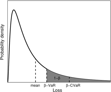
Figure 1: Illustration of VaR and CVaR: $\beta$-VaR is the threshold that the loss exceeds with at most a small probability $1-\beta$. $\beta$-CVaR is the conditional expectation of the loss beyond the $\beta$-VaR.

II CVaR revisited: A Convex Risk Measure

Value-at-risk (VaR) and conditional value-at-risk (CVaR) are widely used in various real-world applications, especially in the finance area, as the popular tools to evaluate the credit risk of a portfolio, and reduce the probability of large losses [30, 31, 32]. The following revisit is useful to grasp their role in the present context.

Consider a loss function $L(\mathbf{x},\bm{\xi}):X\times\Xi\mapsto\mathbb{R}$ denoting the real-valued cost associated with the decision variable $\mathbf{x}\in X\subset\mathbb{R}^{n}$; and the random vector $\bm{\xi}$ with probability density function $p(\bm{\xi})$ supported on a set $\Xi\subset\mathbb{R}^{d}$. In the context of power grids, $\mathbf{x}$ can represent the power schedules of generators, while $\bm{\xi}$ collects the sources of uncertainty due to for instance renewable energy and forecasted load demand.

Clearly, the probability of $L(\mathbf{x},\bm{\xi})$ not exceeding a threshold $\eta$ is given by the right-continuous cumulative distribution function (CDF)

$$\Psi(\mathbf{x},\eta)=\int\limits_{L(\mathbf{x},\bm{\xi})\leq\eta}\!\!p(\bm{\xi})\mathop{}\mathrm{d}\bm{\xi}.$$ (1)

Definition 1 (VaR).

Given a prescribed confidence level $\beta\in(0,1)$, the $\beta$-VaR is the generalized inverse of $\Psi$ defined as

$$\eta_{\beta}(\mathbf{x}) :=\min\{\eta\in\mathbb{R}~{}|~{}\Psi(\mathbf{x},\eta)\geq\beta\}.$$ (2)

$\beta$-VaR is essentially the $\beta$-quantile of the random $L(\mathbf{x},\bm{\xi})$. Since $\Psi$ is non-decreasing in $\eta$, $\eta_{\beta}(\mathbf{x})$ comes out as the lower endpoint of the solution interval satisfying $\Psi(\mathbf{x},\eta)=\beta$, and the commonly chosen values of $\beta$ are, e.g., $0.99$, $0.95$, and $0.9$. Clearly, VaR determines a maximum tolerable loss of an investment, i.e., a threshold the loss will not exceed with a high probability $\beta$. Hence, given the confidence level $\beta$, investors are motivated to solve the so-termed portfolio optimization problem which yields the optimal investment decisions minimizing the VaR value. $\eta_{\beta}(\mathbf{x})$ is proportional to the standard deviation if $\Psi$ is Gaussian. However, for general distributions, $\beta$-VaR is non-subadditive which means the VaR of a combined portfolio can be larger than the sum of the VaRs of each component. This violates the common principle “diversification reduces risk”. Moreover, it is generally non-convex rendering the optimization task hard to tackle.

Because of these conceptual and practical drawbacks, CVaR (a.k.a. “tail VaR”, “mean shortfall”, or “mean excess loss”) was proposed as an alternative risk metric that has many superior properties over VaR.

Definition 2 (CVaR).

The $\beta$-CVaR is the mean of the $\beta$-tail distribution of $L(\mathbf{x},\bm{\xi})$, which is given as

$$\Psi_{\beta}(\mathbf{x},\eta):=\left\{\begin{array}[]{cc}0,&\mbox{if}~{}\eta<\eta_{\beta}(\mathbf{x})\\ \frac{\Psi(\mathbf{x},\eta)-\beta}{1-\beta},&\mbox{if}~{}\eta\geq\eta_{\beta}(\mathbf{x})\end{array}\right.\,.$$ (5)

Truncated and re-scaled from $\Psi$, function $\Psi_{\beta}$ is non-decreasing, right-continuous, and in fact a distribution function. If $\Psi$ is continuous everywhere (without jumps), $\beta$-CVaR coincides with the lower CVaR $\phi_{\beta}^{-}(\mathbf{x}):=\mathbb{E}_{\bm{\xi}}\left[L|L\geq\eta_{\beta}(\mathbf{x})\right]$, that is the conditional expectation of the loss beyond the $\beta$-VaR. Hence, roughly speaking, $\beta$-CVaR is the expected loss in the worst $100(1-\beta)$% scenarios; i.e., cases of such severe losses occur only $100(1-\beta)$ percent of the time.

The $\beta$-CVaR can be also defined as the optimal value of the following optimization problem

$$\phi_{\beta}(\mathbf{x}) :=\min_{\eta\in\mathbb{R}}\left\{\eta+\frac{1}{1-\beta}\mathbb{E}_{\bm{\xi}}\left[L(\mathbf{x},\bm{\xi})-\eta\right]^{+}\right\}.$$ (6)

Let $F_{\beta}(\mathbf{x},\eta)$ denote the objective function in (6). Key properties of $F_{\beta}$ and its relationship with $\eta_{\beta}(\mathbf{x})$ and $\phi_{\beta}(\mathbf{x})$ are summarized next.

Theorem 1 ([31], pp. 1454–1457).

Function $F_{\beta}(\mathbf{x},\eta)$ is finite and convex in $\eta$. Values $\eta_{\beta}(\mathbf{x})$ and $\phi_{\beta}(\mathbf{x})$ are linked through $F_{\beta}(\mathbf{x},\eta)$ as

$$\eta_{\beta}(\mathbf{x}) =\lfloor\operatorname*{arg\,min}_{\eta\in\mathbb{R}}\,F_{\beta}(\mathbf{x},\eta)\rfloor$$ (7)

$$\phi_{\beta}(\mathbf{x}) =F_{\beta}(\mathbf{x},\eta_{\beta}(\mathbf{x}))$$ (8)

$$\min_{\mathbf{x}\in X}\phi_{\beta}(\mathbf{x}) =\min_{(\mathbf{x},\eta)\in X\times\mathbb{R}}F_{\beta}(\mathbf{x},\eta).$$ (9)

Moreover, if $L(\mathbf{x},\bm{\xi})$ is convex in $\mathbf{x}$, then $F_{\beta}(\mathbf{x},\eta)$ is jointly convex in $(\mathbf{x},\eta)$, while $\phi_{\beta}(\mathbf{x})$ is convex in $\mathbf{x}$.

From Definition 2, it can be seen that CVaR is an upper bound of VaR, implying that portfolios with small CVaR also have small VaR. As a consequence of Theorem 1, minimizing the convex $\phi_{\beta}(\mathbf{x})$ amounts to minimizing $F_{\beta}(\mathbf{x},\eta)$, which is not only convex, but also easier to approximate. A readily implementable approximation of the expectation function $F_{\beta}$ is its empirical estimate using $N_{s}$ Monte Carlo samples $\{\bm{\xi}_{s}\}_{s=1}^{N_{s}}$, namely

$$\hat{F}_{\beta}(\mathbf{x},\eta)=\eta+\frac{1}{N_{s}(1-\beta)}\sum_{s=1}^{N_{s}}\left[L(\mathbf{x},\bm{\xi}_{s})-\eta\right]^{+}.$$ (10)

Clearly, the sample average approximation method is distribution free, and the law of large numbers ensures $\hat{F}_{\beta}$ approximates well ${F}_{\beta}$ for $N_{s}$ large enough. Furthermore, $\hat{F}_{\beta}(\mathbf{x},\eta)$ is convex with respect to $(\mathbf{x},\eta)$ if $L(\mathbf{x},\bm{\xi}_{s})$ is convex in $\mathbf{x}$. The non-differentiability due to the projection operator can be readily overcome by leveraging the epigraph form of $\hat{F}$, which will be shown explicitly in Section III-C.

With the function $F_{\beta}(\mathbf{x},\eta)$, it is now possible to develop the CVaR-based stochastic market clearing, as detailed in the next section.

III Stochastic Market Clearing

In a day-ahead electricity market, participants including power generation companies and load service entities (LSEs) first submit their hourly supply bids and demand offers to market operators for the next operating day. Then, the ISO or regional transmission organization (RTO) clear the forward markets yielding least-cost unit commitment decisions, power dispatch outputs, and the corresponding DA clearing prices. The MC procedure proceeds in two stages. A security-constrained unit commitment (SCUC) is performed first by solving a large-scale mixed integer program to commit generation resources after simplifying or omitting transmission constraints. The second stage involves security-constrained economic dispatch (SCED) obtaining the economical power generation outputs and the locational marginal prices (LMPs) as a byproduct. With unit commitment decisions fixed, SCED is usually in the form of DC-OPF, including the transmission network constraints [33].

The MC process is implemented with a goal of minimizing the system net cost, or equivalently maximizing the social welfare. With the trend of increasing penetration of renewables, WPPs are able to directly bid in the forward market [34]. Under uncertainty of wind generation, it now becomes challenging but imperative for the ISOs/RTOs and market participants to extract forecast information and make efficient decisions, including reserve requirements, day-ahead scheduling, market clearing, reliability commitments, as well as the real-time dispatch [35]. In this section, a stochastic MC approach using the CVaR-based transaction cost will be developed as follows.

III-A CVaR-based Energy Transaction Cost

Consider a power system comprising $N_{b}$ buses, $N_{l}$ lines, $N_{g}$ conventional generators, $N_{w}$ wind farms and $N_{a}$ aggregators, each serving a large number of residential end-users with controllable smart appliances. Let ${\cal T}:=\{1,2,\ldots,T\}$ denote the scheduling horizon of interest, e.g., one day ahead. If a wind farm is located at bus $m$, two quantities will be associated with it: the actual wind power generation $w_{m}$, and the power scheduled to be injected $p_{W_{m}}$. Note that the former is random, whereas the latter is a decision variable. For notational simplicity, define also two $N_{w}$-dimensional vectors $\mathbf{w}^{t}:=[w_{1}^{t},\ldots,w_{N_{w}}^{t}]^{\prime}$, and $\mathbf{p}_{W}^{t}:=[p_{W_{1}}^{t},\ldots,p_{W_{N_{w}}}^{t}]^{\prime}$.

Since $\mathbf{w}^{t}$ varies randomly, either energy surplus or shortage should be included to satisfy the nodal balance with the committed quantity $\mathbf{p}_{W}^{t}$. When surplus occurs, the wind farms can sell the excess wind energy back to the spot market, or simply curtail it. For the case of shortage, in order to accomplish the promised bid in the DA contract, farms can buy the energy shortfall from the RT market in the form of ancillary services.

Let $\mathbf{b}^{t}:=[b_{1}^{t},\ldots,b_{N_{w}}^{t}]^{\prime}$ and $\mathbf{s}^{t}:=[s_{1}^{t},\ldots,s_{N_{w}}^{t}]^{\prime}$ collect the purchase and selling prices at time $t$, respectively. Clearly, with the power shortfall and surplus being $[\mathbf{p}_{W}^{t}-\mathbf{w}^{t}]^{+}$ and $[\mathbf{w}^{t}-\mathbf{p}_{W}^{t}]^{+}$ at time $t$, the grid-wide net transaction cost is

$$T(\mathbf{p}_{W},\mathbf{w}) =\sum_{t=1}^{T}\Big{(}\mathbf{b}^{t}\cdot[\mathbf{p}_{W}^{t}-\mathbf{w}^{t}]^{+}-\mathbf{s}^{t}\cdot[\mathbf{w}^{t}-\mathbf{p}_{W}^{t}]^{+}\Big{)}$$

$$=\sum_{t=1}^{T}\Big{(}\bm{\varpi}^{t}\cdot|\mathbf{p}_{W}^{t}-\mathbf{w}^{t}|+\bm{\vartheta}^{t}\cdot(\mathbf{p}_{W}^{t}-\mathbf{w}^{t})\Big{)}$$ (11)

where $\bm{\varpi}^{t}:=\frac{\mathbf{b}^{t}-\mathbf{s}^{t}}{2}$ and $\bm{\vartheta}^{t}:=\frac{\mathbf{b}^{t}+\mathbf{s}^{t}}{2}$; $\mathbf{p}_{W}$ and $\mathbf{w}$ collect $\mathbf{p}_{W}^{t}$ and $\mathbf{w}^{t}$ for all $t\in{\cal T}$, respectively.

Replacing $L(\cdot,\cdot)$ in (6) with $T(\cdot,\cdot)$, function $F_{\beta}$ can be expressed through the conditional expected transaction cost as

$$F_{\beta}(\mathbf{p}_{W},\eta) =\eta+\frac{1}{1-\beta}\mathbb{E}_{\mathbf{w}}\Bigg{[}\sum_{t=1}^{T}\Big{(}\bm{\varpi}^{t}\cdot|\mathbf{p}_{W}^{t}-\mathbf{w}^{t}|$$

$$\hskip 56.9055pt+\bm{\vartheta}^{t}\cdot(\mathbf{p}_{W}^{t}-\mathbf{w}^{t})\Big{)}-\eta\Bigg{]}^{+}.$$ (12)

A condition guaranteeing convexity of $F_{\beta}(\mathbf{p}_{W},\eta)$ is established next.

Proposition 1.

If the selling price $s_{m}^{t}$ does not exceed the purchase price $b_{m}^{t}$ for any $m\in\mathcal{N}_{w}$ and $t\in{\cal T}$, function $F_{\beta}(\mathbf{p}_{W},\eta)$ is jointly convex with respect to $(\mathbf{p}_{W},\eta)$.

Proof:

Thanks to Theorem 1, it suffices to show that $T(\mathbf{p}_{W},\mathbf{w})=\sum_{t=1}^{T}\Big{(}\bm{\varpi}^{t}\cdot|\mathbf{p}_{W}^{t}-\mathbf{w}^{t}|+\bm{\vartheta}^{t}\cdot(\mathbf{p}_{W}^{t}-\mathbf{w}^{t})\Big{)}$ is convex in $\mathbf{p}_{W}$ under the proposition’s condition. Clearly, the stated condition is equivalent to $\bm{\varpi}^{t}\succeq\mathbf{0}$ for all $t\in{\cal T}$. Thus, by the convexity of the absolute value function, and the convexity-preserving operators of summation and expectation [36, Sec. 3.2], the claim follows readily. ∎

In this paper, a perfectly competitive market is assumed such that all participants act as price takers. That is, every competitor is atomistic to have small enough market share so that there is no market power affecting the price [37]. For American electricity markets, a single pricing mechanism is used such that $\mathbf{s}^{t}\equiv\mathbf{b}^{t}$ holds in most of the scenarios. This is a special case of the pricing condition in Prop. 1, which facilitates calculating the function (12) since the absolute value functions vanish. Note that it is possible that different WPPs may buy (sell) wind energy from (to) different sellers (purchasers) in a competitive electricity pool as an ancillary service, which can yield different purchase and selling prices.

For most of the European markets including UK, France, Italy, and Netherlands, the imbalance prices $\{\mathbf{b}^{t},\mathbf{s}^{t}\}_{t}$ are commonly set in an ex-post way that is known as dual imbalance pricing [38]. Specifically, if the system RT imbalance is negative, i.e., the overall market is short, then $\mathbf{s}^{t}=\bm{\chi}^{t}\preceq\mathbf{b}^{t}$ holds, where $\bm{\chi}^{t}:=[\chi_{1}^{t},\ldots,\chi_{N_{w}}^{t}]^{\prime}$ collects the DA prices at the buses attached with all $N_{w}$ wind farms. In this case, the RT purchase price is typically higher than the DA price, reflecting the cost of acquiring the balancing energy [39]. Wind farms with excess energy can sell this part to reduce the system imbalance but only be paid the DA prices. On the other hand, we have $\mathbf{s}^{t}\preceq\bm{\chi}^{t}=\mathbf{b}^{t}$ if the market is long. Hence, market participants selling excess energy receive a balancing price which is lower than the DA one, while those running negative imbalance pay the DA price. Note that the relationship $\mathbf{s}^{t}\preceq\bm{\chi}^{t}\preceq\mathbf{b}^{t}$ always holds even when the market imbalance outcome is unknown at the time of the DA bids. Such a pricing mechanism drives bidders to match their forward offers with the true forecasts of generation or consumption.

Leveraging the CVaR-based transaction cost, a stochastic MC problem based on the DC-OPF will be formulated next.

III-B CVaR-based Market Clearing

Let $\mathbf{p}_{G}^{t}:=[P_{G_{1}}^{t},\ldots,P_{G_{N_{g}}}^{t}]^{\prime}$ and $\mathbf{p}_{\mathrm{DRA}}^{t}:=[P_{\mathrm{DRA}_{1}}^{t},\ldots,P_{\mathrm{DRA}_{N_{a}}}^{t}]^{\prime}$ denote the power outputs of the thermal generators, and the power consumption of the aggregators at slot $t$, respectively. Define further the sets $\mathcal{N}_{a}:=\{1,2,\ldots,N_{a}\}$ and $\mathcal{N}_{g}:=\{1,2,\ldots,N_{g}\}$. Each aggregator $j\in\mathcal{N}_{a}$ serves a set $\mathcal{R}_{j}$ of residential users, and each user $r\in\mathcal{R}_{j}$ has a set $\mathcal{S}_{rj}$ of controllable appliances. Let $\mathbf{p}_{jrs}$ be the power consumption of appliance $s$ with user $r$ corresponding to aggregator $j$ across the slots. The operational constraints of $\mathbf{p}_{jrs}$ are captured by a set $\mathcal{P}_{jrs}$, while the end user satisfaction is modeled by a concave utility function $U_{jrs}(\mathbf{p}_{jrs})$. Furthermore, let convex functions $\{C_{i}(\cdot)\}_{i}$ denote the generation costs, and $\mathbf{p}_{\mathrm{BL}}^{t}$ the base load demand. For brevity, let vector $\mathbf{p}_{0}$ collect variables $\eta$ and $\{\mathbf{p}_{G}^{t},\mathbf{p}_{\mathrm{DRA}}^{t},\mathbf{p}_{W}^{t},\bm{\theta}^{t}\}_{t\in{\cal T}}$; and vector $\{\mathbf{p}_{j}\}_{j\in\mathcal{N}_{a}}$ the power consumption of all appliances with the aggregator $j$.

Hinging on three assumptions: a1) lossless lines, a2) small voltage phase differences, and a3) approximated one p.u. voltage magnitudes, the DC-OPF based stochastic MC stands with the goal of minimizing the social cost:

$$\min\sum_{t=1}^{T}\sum_{i=1}^{N_{g}}C_{i}(P_{G_{i}}^{t})-\sum_{j=1}^{N_{a}}\sum_{\begin{subarray}{c}r\in\mathcal{R}_{j},\\ s\in\mathcal{S}_{jr}\end{subarray}}U_{jrs}(\mathbf{p}_{jrs})+\mu F_{\beta}(\mathbf{p}_{W},\eta)$$ (13a)

$$\mathrm{subject~{}to:}$$

$$\mathbf{A}_{g}\mathbf{p}_{G}^{t}+\mathbf{A}_{w}\mathbf{p}_{W}^{t}-\mathbf{A}_{a}\mathbf{p}_{\mathrm{DRA}}^{t}-\mathbf{p}_{\mathrm{BL}}^{t}=\mathbf{B}_{n}\bm{\theta}^{t},~{}t\in{\cal T}$$ (13b)

$$P_{G_{i}}^{\min}\leq P_{G_{i}}^{t}\leq P_{G_{i}}^{\max},~{}i\in\mathcal{N}_{g},~{}t\in{\cal T}$$ (13c)

$$-\mathsf{R}_{i}^{\mathrm{down}}\leq P_{G_{i}}^{t}-P_{G_{i}}^{t-1}\leq\mathsf{R}_{i}^{\mathrm{up}},~{}i\in\mathcal{N}_{g},\>t\in{\cal T}$$ (13d)

$$\mathbf{f}^{\min}\preceq\mathbf{B}_{f}\bm{\theta}^{t}\preceq\mathbf{f}^{\max},~{}t\in{\cal T}$$ (13e)

$$\theta_{1}^{t}=0,\>t\in{\cal T}$$ (13f)

$$\mathbf{0}\preceq\mathbf{p}_{W}\preceq\mathbf{p}_{W}^{\mathrm{max}}$$ (13g)

$$0\leq P_{\mathrm{DRA}_{j}}^{t}\leq P_{\mathrm{DRA}_{j}}^{\max},~{}j\in\mathcal{N}_{a},\,t\in{\cal T}$$ (13h)

$$P_{\mathrm{DRA}_{j}}^{t}=\sum\nolimits_{r\in\mathcal{R}_{j},\,s\in\mathcal{S}_{jr}}{p}_{jrs}^{t},~{}j\in\mathcal{N}_{a},\>t\in{\cal T}$$ (13i)

$$\mathbf{p}_{jrs}\in\mathcal{P}_{jrs},~{}s\in\mathcal{S}_{jr},~{}r\in\mathcal{R}_{j},~{}j\in\mathcal{N}_{a}$$ (13j)

$$\mathrm{variables:}\,\,\{\mathbf{p}_{j}\}_{j=0}^{N_{a}}$$

where the nodal susceptance matrix $\mathbf{B}_{n}:=-\mathbf{A}_{n}^{\prime}\mathbf{B}_{s}\mathbf{A}_{n}\in\mathbb{R}^{N_{b}\times N_{b}}$ and the angle-to-flow matrix $\mathbf{B}_{f}:=-\mathbf{B}_{s}\mathbf{A}_{n}\in\mathbb{R}^{N_{l}\times N_{b}}$. The $\ell$th row of the branch-node incidence matrix $\mathbf{A}_{n}\in\mathbb{R}^{N_{l}\times N_{b}}$ has $1$ and $-1$ in its entry corresponding to the from and to nodes of branch $\ell$, and $0$ elsewhere; and the square diagonal matrix $\mathbf{B}_{s}:=\mathrm{diag}(b_{1},\ldots,b_{N_{l}})$ is the branch susceptance matrix collecting the primitive susceptance across all branches.

Matrices $\mathbf{A}_{g}\in\mathbb{R}^{N_{b}\times N_{g}}$, $\mathbf{A}_{w}\in\mathbb{R}^{N_{b}\times N_{w}}$ and $\mathbf{A}_{a}\in\mathbb{R}^{N_{b}\times N_{a}}$ in (13b) are the incidence matrices of the conventional generators, the wind farms, and the aggregators, respectively. Take $\mathbf{A}_{g}$ as an example, $(\mathbf{A}_{g})_{mn}=1$ if the $n$th generator is injected to the $m$th bus, and $(\mathbf{A}_{g})_{mn}=0$, otherwise. Matrices $\mathbf{A}_{w}$ and $\mathbf{A}_{a}$ can be constructed likewise. Consider the power network in Fig. 2 adapted from the Western Electricity Coordinating Council (WECC) system [40]. With $N_{b}=6$, $N_{l}=6$, $N_{g}=3$, and $N_{a}=4$, matrices $\mathbf{A}_{g}$, $\mathbf{A}_{w}$, and $\mathbf{A}_{a}$ take the following form:

$$\mathbf{A}_{g}=\begin{bmatrix}1&0&0\\ 0&1&0\\ 0&0&1\\ 0&0&0\\ 0&0&0\\ 0&0&0\end{bmatrix},\mathbf{A}_{w}=\begin{bmatrix}1&0&0\\ 0&1&0\\ 0&0&0\\ 0&0&0\\ 0&0&1\\ 0&0&0\end{bmatrix},\mathbf{A}_{a}=\begin{bmatrix}0&0&0&0\\ 0&0&0&0\\ 0&0&0&0\\ 1&1&0&0\\ 0&0&1&0\\ 0&0&0&1\end{bmatrix}.$$

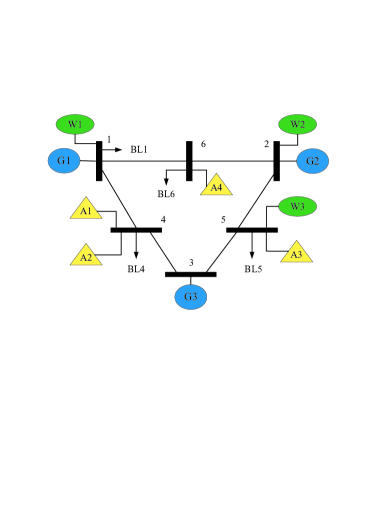
Figure 2: Modified WECC system featuring 6 buses, 3 generators, 4 aggregators, 4 base loads, and 3 wind farms.

A smart appliance example is charging a plug-in hybrid electric vehicle (PHEV), which typically amounts to consuming a prescribed total energy $E_{jrs}$ over a specific horizon from a start time $T_{jrs}^{\mathrm{st}}$ to a termination time $T_{jrs}^{\mathrm{end}}$. The consumption must remain within a range between $p_{jrs}^{\mathrm{min}}$ and $p_{jrs}^{\mathrm{max}}$ per period. With $\mathcal{T}_{jrs}^{E}:=\{T_{jrs}^{\mathrm{st}},\ldots,T_{jrs}^{\mathrm{end}}\}$, set $\mathcal{P}_{jrs}$ takes the form:

$$\mathcal{P}_{jrs}=\Biggl{\{}\mathbf{p}_{jrs} \Biggl{|}\Biggr{.}\sum_{t\in\mathcal{T}_{jrs}^{E}}{p}_{jrs}^{t}=E_{jrs},\,p_{jrs}^{t}\in[p_{jrs}^{\mathrm{min}},p_{jrs}^{\mathrm{max}}],$$

$$\forall~{}t\in\mathcal{T}_{jrs}^{E};\,p_{jrs}^{t}=0,~{}\forall~{}t\in{\cal T}\setminus\mathcal{T}_{jrs}^{E}\Biggr{\}}.$$ (14)

Further examples of $\mathcal{P}_{jrs}$ and $U_{jrs}(\mathbf{p}_{jrs})$ can be found in [17], where it is argued that $\mathcal{P}_{jrs}$ is a convex set for several appliance types of interest.

Linear equality (13b) is the nodal balance constraint; i.e., the load balance at bus levels dictated by the law of conservation of power. Limits of generator outputs and ramping rates are specified in constraints (13c) and (13d). Network power flow constraints are accounted for in (13e). Without loss of generality, the first bus can be set as the reference bus with zero phase in (13f). Constraints (13h) and (13g) capture the lower and upper limits of the energy consumed by the aggregators and the committed wind power, respectively. Equality (13i) amounts to the aggregator-user power balance equation; and constraints (13j) define the feasible set of appliances. Finally, the pre-determined risk-aversion parameter $\mu>0$ controls the trade off between the transaction cost and the generation cost as well as the end-user utility.

Remark 1.

(Availability of real-time prices). In this paper, the real-time prices $\{\mathbf{b}^{t},\mathbf{s}^{t}\}_{t\in{\cal T}}$ are assumed to be perfectly known to the ISO for the DA market clearing. However, such an assumption can be readily extended to a more practical setup by taking the price stochasticity into account. Specifically, imperfect price information can be modeled by appropriately designing the function $T(\mathbf{p}_{W},\mathbf{w})$ [cf. (11)]. For example, the expectation can be also taken over the random RT prices in (12) as $F_{\beta}(\mathbf{p}_{W},\eta)=\eta+\frac{1}{1-\beta}\mathbb{E}_{\{\mathbf{w},\{\mathbf{b}^{t},\mathbf{s}^{t}\}_{t}\}}[T(\mathbf{p}_{W},\mathbf{w})-\eta]^{+}$. The dependence between $\{\mathbf{b}^{t},\mathbf{s}^{t}\}$ and $\mathbf{w}$ can be further investigated. In addition, worst-case analysis is available upon postulating an uncertainty set $\Delta$ for $\{\mathbf{b}^{t},\mathbf{s}^{t}\}$. This results in a novel risk measure given as $F_{\beta}(\mathbf{p}_{W},\eta)=\eta+\frac{1}{1-\beta}\mathbb{E}_{\mathbf{w}}[\sup_{\{\mathbf{b}^{t},\mathbf{s}^{t}\}_{t}\in\Delta}T(\mathbf{p}_{W},\mathbf{w})-\eta]^{+}$.

It is worth mentioning that SCED and SCUC yield two different market pricing systems: locational marginal pricing and convex hull pricing (a.k.a. extended LMP). The ED formulation produces the LMPs given by the dual variables associated with the supply-demand balance constraint. Prices supporting the equilibrium solution are found at the intersection of the supply marginal cost curve with the demand bids. However, if discrete operations of UC are involved, there is no exact price that supports such an economic equilibrium. This issue prompted the introduction of the convex hull pricing to reduce the uplift payments [41]. In the present paper, the core ED model is considered to deal with the high penetration of renewables and large-scale DR programs. Therefore, the formulation (13) relies on re-solving the dispatch problem with fixed UC decisions.

$$L_{\rho}(\mathbf{x},\mathbf{y},\bm{\lambda})= \sum_{t=1}^{T}\sum_{i=1}^{N_{g}}C_{i}(P_{G_{i}}^{t})-\sum_{j=1}^{N_{a}}\sum_{\begin{subarray}{c}r\in\mathcal{R}_{j},\\ s\in\mathcal{S}_{jr}\end{subarray}}U_{jrs}(\mathbf{p}_{jrs})+\mu\left(\eta+\frac{\sum_{s=1}^{Ns}u_{s}}{N_{s}(1-\beta)}\right)$$

$$+ \sum_{t=1}^{T}\sum_{j=1}^{N_{a}}\lambda_{j}^{t}\left(P_{\mathrm{DRA}_{j}}^{t}-\sum_{r,s}{p}_{jrs}^{t}\right)+\frac{\rho}{2}\sum_{t=1}^{T}\sum_{j=1}^{N_{a}}\left(P_{\mathrm{DRA}_{j}}^{t}-\sum_{r,s}{p}_{jrs}^{t}\right)^{2}$$ (16)

Remark 2.

(Reliability assessment commitment). The proposed dispatch model can be cast as a two-stage program. The first stage is the DA MC, and the second is simply the balancing operation (recourse action) dealing with differences between the pre-dispatch amount and the actual wind power generation. Between the DA and RT markets, ISOs implement the reliability assessment commitment (RAC) as a reliability backstop tool to ensure sufficient resources are available and cover the adjusted forecast load online. One principle of the RAC process is to commit the capacity deemed necessary to reliably operate the grid at the least commitment cost. In this step, based on the updated information of the wind power forecast, WPPs have an opportunity to feedback to the ISO if they are able to commit the scheduled wind power decided by the DA MC. Then, the ISO is able to adjust UC decisions as necessary to ensure reliability.

To this end, reformulation of problem (13) as a smooth convex minimization is useful for developing distributed solvers, as detailed next.

III-C Smooth Convex Minimization Reformulation

It is clear that under the condition of Proposition 1, the objective and the constraints of (13) are convex, which renders it not hard to solve in principle. Nevertheless, due to the high-dimensional integration present in $F_{\beta}(\mathbf{p}_{W},\eta)$ [cf. (12)], an analytical solution is typically impossible. To this end, it is necessary to re-write the resulting problem in a form suitable for off-the-shelf solvers.

First, as shown in (10), an efficient approximation of $F_{\beta}(\mathbf{p}_{W},\eta)$ is offered by the empirical expectation using i.i.d. samples $\{\mathbf{w}_{s}\}_{s=1}^{N_{s}}$; that is,

$$\hat{F}_{\beta}(\mathbf{p}_{W},\eta) =\eta+\frac{1}{N_{s}(1-\beta)}\sum_{s=1}^{N_{s}}\Bigg{[}\sum_{t=1}^{T}\Big{(}\bm{\varpi}^{t}\cdot|\mathbf{p}_{W}^{t}-\mathbf{w}_{s}^{t}|$$

$$\hskip 56.9055pt+\bm{\vartheta}^{t}\cdot(\mathbf{p}_{W}^{t}-\mathbf{w}_{s}^{t})\Big{)}-\eta\Bigg{]}^{+}.$$ (15)

Next, by introducing auxiliary variables $\{u_{s}\}_{s=1}^{Ns}$, the non-smooth convex program (13) can be equivalently re-written as the following smooth convex minimization:

$$\min\sum_{t=1}^{T}\sum_{i=1}^{N_{g}}C_{i}(P_{G_{i}}^{t})-\sum_{j=1}^{N_{a}}\sum_{\begin{subarray}{c}r\in\mathcal{R}_{j},\\ s\in\mathcal{S}_{jr}\end{subarray}}U_{jrs}(\mathbf{p}_{jrs})$$

$$\hskip 99.58464pt+\mu\left(\eta+\frac{\sum_{s=1}^{Ns}u_{s}}{N_{s}(1-\beta)}\right)$$ (16a)

$$\mathrm{subject~{}to:}\,\,\eqref{eq:mc-bus}-\eqref{eq:mc-appl}$$

$$\sum_{t=1}^{T}\Big{(}\bm{\varpi}^{t}\cdot|\mathbf{p}_{W}^{t}-\mathbf{w}_{s}^{t}|+\bm{\vartheta}^{t}\cdot(\mathbf{p}_{W}^{t}-\mathbf{w}_{s}^{t})\Big{)}\leq u_{s}+\eta,\,$$

$$\hskip 170.71652pts\in\mathcal{N}_{s}$$ (16b)

$$\mathrm{variables:}\,\,\{\mathbf{p}_{j}\}_{j=0}^{N_{a}},\,\{u_{s}\in\mathbb{R}_{+}\}_{s=1}^{N_{s}}.$$

Under mild conditions, the optimal solution set of (16) converges exponentially fast to its counterpart of (13), as the sample size $N_{s}$ increases. The proof is based on the theory of large deviations [42], but is omitted here due to space limitations.

Problem (16) can be solved centrally at the ISO in principle. However, with large-scale DR, distributed solvers are well motivated not only for computational efficiency but also for privacy reasons. Specifically, functions $U_{jrs}(\mathbf{p}_{jrs})$ and sets $\{\mathcal{P}_{jrs}\}$ are private, and are not revealed to the ISO; and (ii) the operational sets $\{\mathcal{P}_{jrs}\}_{j,r,s}$ of very large numbers of heterogenous appliances may become prohibitively complicated; e.g., mix-integer constraints can even be involved to model the ON/OFF status and un-interruptible operating time of end-user appliances [43, 44]. This renders the overall problem intractable for the ISO. To this end, the DR aggregators can play a critical role to split the resulting optimization task as detailed next.

IV Distributed Market Clearing via ADMM

Selecting how to decompose the optimization task as well as updating the associated multipliers are crucial for the distributed design. Fewer updates simply imply lower communication overhead between the ISO and the aggregators. One splitting approach is the dual decomposition with which the dual subgradient ascent algorithm is typically very slow. Instead, a fast-convergent solver via the ADMM [45] is adapted in this section for the distributed MC.

IV-A The ADMM Method

Consider the following separable convex minimization problem with linear equality constraints:

$$\min_{\mathbf{x}\in\mathcal{X},\mathbf{y}\in\mathcal{Y}}~{} f(\mathbf{x})+g(\mathbf{y})$$ (17a)

$$\mathrm{subject~{}to:}\quad \mathbf{A}\mathbf{x}+\mathbf{B}\mathbf{y}=\mathbf{c}.$$ (17b)

For the stochastic MC problem (16), the primal variable $\mathbf{x}$ comprises the group $\{u_{s}\}_{s\in\mathcal{N}_{s}}$ and $\mathbf{p}_{0}$, while $\mathbf{y}$ collects $\{\mathbf{p}_{j}\}_{j\in\mathcal{N}_{a}}$. Hence, set $\mathcal{X}$ captures constraints (13b)–(13h) and (16b) while $\mathcal{Y}$ represents (13j). The linear equality constraint (17b) corresponds to (13i).

Let $\bm{\lambda}:=[\lambda_{1}^{1},\ldots,\lambda_{N_{a}}^{T}]^{\prime}\in\mathbb{R}^{TN_{a}}$ denote the Lagrange multiplier vector associated with the constraint (13i). The partially augmented Lagrangian of (16) is thus given by (16), where the weight $\rho>0$ is a penalty parameter controlling the violation of primal feasibility, which turns out to be the step size of the dual update. As the iterative solver of (16) proceeds, the primal residual converges to zero that ensures optimality. Judiciously selecting $\rho$ thus strikes a desirable tradeoff between the size of primal vis-à-vis dual residuals. Note also that by varying $\rho$ over a finite number of iterations may improve convergence [45]. In a nutshell, finding the “optimal” value of $\rho$ is generally application-dependent that requires a trial-and-error tuning.

Different from [46] where the power balance and phase consistency constraints are relaxed, in this work only the aggregator-user power balance equation (13i) is dualized so that the nodal balance equation (13b) is kept in the subproblem of the ISO. Decomposing the problem (16) in such a way can reduce the heavy computational burden at the ISO while respect the privacy of end users within each aggregator. The ADMM iteration cycles between primal variable updates using block coordinate descent (a.k.a. Gauss-Seidel), and dual variable updates via gradient ascent. The resulting distributed MC is tabulated as Algorithm 1, where $k$ is the iteration index. The last step is a reasonable termination criterion based on the primal residual [45, Sec. 3.3.1]

$$\xi:=\left[\sum_{t=1}^{T}\sum_{j=1}^{N_{a}}\left(P_{\mathrm{DRA}_{j}}^{t}-\sum_{r,s}{p}_{jrs}^{t}\right)^{2}\right]^{1/2}.$$ (17)

Algorithm 1 ADMM-based Distributed Market Clearing

1:Initialize $\bm{\lambda}(0)=\mathbf{0}$

2:repeat for $k=0,1,2,\ldots$

3:     update primal variables:

$$\mathbf{x}(k+1) =\operatorname*{arg\,min}_{\mathbf{x}\in\mathcal{X}}~{}L_{\rho}(\mathbf{x},\mathbf{y}(k),\bm{\lambda}(k))$$ (18)

$$\mathbf{y}(k+1) =\operatorname*{arg\,min}_{\mathbf{y}\in\mathcal{Y}}~{}L_{\rho}(\mathbf{x}(k+1),\mathbf{y},\bm{\lambda}(k))$$ (19)

4:     update dual variables: for all $j\in\mathcal{N}_{a}$ and $t\in\mathcal{T}$

$$\lambda_{j}^{t}(k+1)=\lambda_{j}^{t}(k)+\rho\big{(}P_{\mathrm{DRA}_{j}}^{t}(k+1)-\sum_{r,s}{p}_{jrs}^{t}(k+1)\big{)}$$ (20)

5:until $\xi\leq\epsilon^{\mathrm{pri}}$

Specifically, given the Lagrangian multipliers $\bm{\lambda}(k)$ and the power consumption $\{\mathbf{p}_{jrs}(k)\}_{jrs}$ of the end-user appliances, The ISO solves the convex subproblem (18) given as follows:

$$\mathbf{p}_{0}(k+1)=\operatorname*{arg\,min}_{\mathbf{p}_{0},\{u_{s}\}}\sum_{\begin{subarray}{c}t\in{\cal T},\\ i\in\mathcal{N}_{g}\end{subarray}}C_{i}(P_{G_{i}}^{t})+\mu\left(\eta+\frac{\sum_{s=1}^{Ns}u_{s}}{N_{s}(1-\beta)}\right)$$

$$+\sum_{\begin{subarray}{c}t\in{\cal T},\\ j\in\mathcal{N}_{a}\end{subarray}}\lambda_{j}^{t}(k)P_{\mathrm{DRA}_{j}}^{t}+\frac{\rho}{2}\sum_{\begin{subarray}{c}t\in{\cal T},\\ j\in\mathcal{N}_{a}\end{subarray}}\left(P_{\mathrm{DRA}_{j}}^{t}-\sum_{r,s}{p}_{jrs}^{t}(k)\right)^{2}$$ (21a)

$$\mathrm{subject\,to:}$$

$$\mathbf{A}_{g}\mathbf{p}_{G}^{t}+\mathbf{A}_{w}\mathbf{p}_{W}^{t}-\mathbf{A}_{a}\mathbf{p}_{\mathrm{DRA}}^{t}-\mathbf{p}_{\mathrm{BL}}^{t}=\mathbf{B}_{n}\bm{\theta}^{t},~{}t\in{\cal T}$$ (21b)

$$P_{G_{i}}^{\min}\leq P_{G_{i}}^{t}\leq P_{G_{i}}^{\max},~{}i\in\mathcal{N}_{g},~{}t\in{\cal T}$$ (21c)

$$-\mathsf{R}_{i}^{\mathrm{down}}\leq P_{G_{i}}^{t}-P_{G_{i}}^{t-1}\leq\mathsf{R}_{i}^{\mathrm{up}},~{}i\in\mathcal{N}_{g},\>t\in{\cal T}$$ (21d)

$$\mathbf{f}^{\min}\preceq\mathbf{B}_{f}\bm{\theta}^{t}\preceq\mathbf{f}^{\max},~{}t\in{\cal T}$$ (21e)

$$\theta_{1}^{t}=0,\>t\in{\cal T}$$ (21f)

$$\mathbf{0}\preceq\mathbf{p}_{W}\preceq\mathbf{p}_{W}^{\mathrm{max}}$$ (21g)

$$0\leq P_{\mathrm{DRA}_{j}}^{t}\leq P_{\mathrm{DRA}_{j}}^{\max},~{}j\in\mathcal{N}_{a},\,t\in{\cal T}$$ (21h)

$$\sum_{t=1}^{T}\Big{(}\bm{\varpi}^{t}\cdot|\mathbf{p}_{W}^{t}-\mathbf{w}_{s}^{t}|+\bm{\vartheta}^{t}\cdot(\mathbf{p}_{W}^{t}-\mathbf{w}_{s}^{t})\Big{)}\leq u_{s}+\eta,\,$$

$$\text{and}\,\,u_{s}\geq 0,\,\,s\in\mathcal{N}_{s}.$$ (21i)

Interestingly, (19) is decomposable so that $\{\mathbf{p}_{jrs}(k)\}_{r,s}$ can be separately solved by each aggregator:

$$\{\mathbf{p}_{jrs}(k+1)\}_{r,s}=\operatorname*{arg\,min}_{\{\mathbf{p}_{jrs}\}_{r,s}}\,\,-\sum_{t=1}^{T}\lambda_{j}^{t}(k)\sum_{r,s}{p}_{jrs}^{t}$$

$$-\sum_{\begin{subarray}{c}r\in\mathcal{R}_{j},\\ s\in\mathcal{S}_{jr}\end{subarray}}U_{jrs}(\mathbf{p}_{jrs})+\frac{\rho}{2}\sum_{t=1}^{T}\left(\sum_{r,s}{p}_{jrs}^{t}-P_{\mathrm{DRA}_{j}}^{t}(k+1)\right)^{2}$$ (22a)

$$\mathrm{subject~{}to:}\,\,\{\mathbf{p}_{jrs}\in\mathcal{P}_{jrs}\}_{r,s}.$$ (22b)

Having found $\mathbf{p}_{0}(k)$ and $\{\mathbf{p}_{jrs}(k)\}_{jrs}$, the multipliers $\{\mu_{j}^{t}\}_{j,t}$ are updated using gradient ascent as in (20). To solve the convex problem (22), each aggregator must collect the corresponding users’ information including $U_{jrs}$ and $\mathcal{P}_{jrs}$. This is implementable via the advanced metering infrastructure [47].

Remark 3.

(Distributed demand response). It must be further pointed out that the quadratic penalty $\big{(}P_{\mathrm{DRA}_{j}}^{t}-\sum_{r,s}{p}_{jrs}^{t}\big{)}^{2}$ in (16) couples load consumptions $\{{p}_{jrs}^{t}\}$ over different residential users. Hence, the ADMM-based distributed solver may not be applicable whenever ${p}_{jrs}^{t}$ must be updated per end user rather than the aggregator. This may arise either to strictly protect the privacy of end users from DR aggregators, or, to accommodate large-scale DR programs where each aggregator cannot even afford solving the subproblem (22). In this case, leveraging the plain Lagrangian function (no coupling term), the dual decomposition based schemes can be utilized by end users to separately update $\{{p}_{jrs}^{t}\}$ in parallel; see e.g., [17] and [48].

The convergence of the ADMM solver and its implications for the market price are discussed next.

IV-B Pricing Impacts

Suppose two additional conditions hold for the convex problem (16): c1) functions $\{C_{i}(\cdot)\}_{i}$ and $\{-U_{jrs}(\cdot)\}_{jrs}$ are closed and proper convex; and c2) the plain Lagrangian $L_{0}$ has a saddle point. Then, the ADMM iterates of the objective (16a) and the dual variables $\{\lambda_{j}^{t}\}_{j,t}$ are guaranteed to converge to the optimum [45]. In addition, if the objective is strongly convex, then the primal variable iterates including $\mathbf{p}_{G}$, $\mathbf{p}_{\mathrm{DRA}}$, $\mathbf{p}_{W}$ and $\{\mathbf{p}_{j}\}_{j\in\mathcal{N}_{a}}$ converge to the globally optimal solutions.

The guaranteed convergence of the dual variables also facilitates the calculation of LMPs. Let $\bar{\bm{\lambda}}^{t}:=[\bar{\lambda}_{1}^{t},\ldots,\bar{\lambda}_{N_{a}}^{t}]^{\prime}$ and $\bar{\bm{\tau}}^{t}:=[\bar{\tau}_{1}^{t},\ldots,\bar{\tau}_{N_{b}}^{t}]^{\prime}$ denote the optimal Lagrange multipliers associated with the aggregator-user balance constraint (13i), and the nodal balance constraint (13b), respectively. Note that with the optimal solutions $\bar{\bm{\lambda}}^{t}$ and $\{\bar{\mathbf{p}}_{jrs}\}_{jrs}$ obtained by the ADMM solver, the LMPs $\{\bar{\bm{\tau}}^{t}\}_{t}$ can be found by solving the subproblem (21) with primal-dual algorithms. In addition, if $0<P_{\mathrm{DRA}_{j}}^{t}<P_{\mathrm{DRA}_{j}}^{\max},\forall j,t$ holds at the optimal solution $\bar{P}_{\mathrm{DRA}_{j}}^{t}$, then $\bar{\bm{\lambda}}^{t}=\mathbf{A}_{a}^{\prime}\bar{\bm{\tau}}^{t}$; i.e., $\bar{\lambda}_{j}^{t}=\bar{\tau}_{n}^{t}$ for all aggregators $j$ attached with bus $n$ (see also [17]). To this end, payments of the market participants can be calculated with the obtained LMPs and optimal DA dispatches. In the RT market of a two-settlement system, if the supplier at bus $n$ delivers $\tilde{P}_{G_{n}}^{t}$ with the real-time price $\tilde{\tau}_{n}^{t}$, then the supplier gets paid

$$\Pi_{G_{n}}=\sum_{t=1}^{T}\bar{\tau}_{n}^{t}\bar{P}_{G_{n}}^{t}+\tilde{\tau}_{n}^{t}(\tilde{P}_{G_{n}}^{t}-\bar{P}_{G_{n}}^{t}).$$

Likewise, the aggregator at bus $n$ needs to pay

$$\Pi_{\textrm{DRA}_{n}}=\sum_{t=1}^{T}\bar{\tau}_{n}^{t}\bar{P}_{\textrm{DRA}_{n}}^{t}+\tilde{\tau}_{n}^{t}(\tilde{P}_{\textrm{DRA}_{n}}^{t}-\bar{P}_{\textrm{DRA}_{n}}^{t}).$$

The revenue of the wind farm at bus $n$ is

$$\Pi_{W_{n}}=\sum_{t=1}^{T}\big{(}\bar{\tau}_{n}^{t}\bar{p}_{W_{n}}^{t}+s_{n}^{t}[w_{n}^{t}-\bar{p}_{W_{n}}^{t}]^{+}-b_{n}^{t}[\bar{p}_{W_{n}}^{t}-w_{n}^{t}]^{+}\big{)}.$$

Remark 4.

(Pricing consistence). In a perfectly competitive market, any arbitrage opportunities between the DA and RT markets are exploited by market participants. Hence, the DA nodal prices are consistent with the DT nodal prices meaning the expectations of the latter converge to the former. The concepts of price distortions and revenue adequacy have been recently proposed for the stochastic MC in [49]. In the setup of a single snapshot therein, it has been proved that the medians and expectations of RT prices converge to the DA counterparts for the $\ell_{1}$ and $\ell_{2}$ penalties between the RT and DA power schedules, respectively. Building upon this solid result, it is possible to establish bounded price distortions for the proposed model, while its consistent pricing property can also be analyzed in a similar fashion. The involved important analysis is however beyond the scope of this paper, and is left for future work.

V Numerical Tests

TABLE I: Conventional generator parameters. The units of $a_{i}$ and $b_{i}$ are $/(MWh)² and $/MWh, respectively. the rest are in MW.

Unit	$a_{i}$	$b_{i}$	$P_{G_{i}}^{\max}$	$P_{G_{i}}^{\min}$	$\mathsf{R}_{i}^{\mathrm{up}}$	$\mathsf{R}_{i}^{\mathrm{down}}$
1	0.3	50	90	10	50	50
2	0.15	30	50	5	35	40
3	0.2	40	60	8	40	40

TABLE II: Parameters of PHEVs. All listed hours are the ending ones; w.p. means with probability.

$E_{\mathrm{PHEV}}$ (kWh)	Uniform on {10, 11, 12}
$p_{\mathrm{PHEV}}^{\max}$ (kWh)	Uniform on {2.1, 2.3, 2.5}
$p_{\mathrm{PHEV}}^{\min}$ (kWh)	0
$T_{jrs}^{\mathrm{st}}$	1am
$T_{jrs}^{\mathrm{end}}$	6am w.p. 70%, 7am w.p. 30%

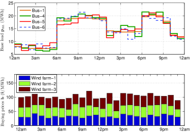
Figure 3: Fixed base load demand $\{\mathbf{p}_{\text{BL}}^{t}\}$ and energy purchase prices $\{\mathbf{b}^{t}\}$.

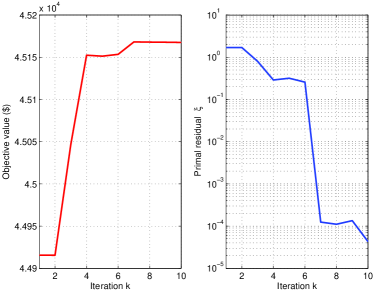
Figure 4: Convergence of the objective value (16a) and the primal residual (17).

In this section, simulated tests are presented to verify the merits of the proposed CVaR-based MC. The tested power system is modified from the WECC system as illustrated in Fig. 2. Each of the $4$ DR aggregators serves $200$ residential customers. The scheduling horizon starts from $12$am until $23$pm, a total of $24$ hours

Time-invariant generation cost functions were chosen quadratic as $C_{i}(P_{G_{i}}^{t})=a_{i}(P_{G_{i}}^{t})^{2}+b_{i}P_{G_{i}}^{t}$ for all $i$ and $t$. For simplicity, each end user has one PHEV to charge from midnight. All detailed parameters of the conventional generators and loads are listed in Tables I and II. The upper bound of each aggregator’s consumption is $P_{\mathrm{DRA}_{j}}^{\max}=50$ MW. At a base of $100\text{\,}\mathrm{M}\mathrm{V}\mathrm{A}$, the values of the network reactances are $\{X_{16},X_{62},X_{25},X_{53},X_{34},X_{41}\}=\{0.2,0.3,0.25,0.1,0.3,0.4\}$ p.u. Finally, no flow limits were imposed, while the utility functions $\{U_{jrs}(\cdot)\}$ were set to zero. The resulting convex programs (21) and (22) were modeled using the Matlab-based package CVX [50], and solved by SeDuMi [51].

Variable characteristics of the daily power market are captured via two groups of parameters shown in Fig. 3: the fixed base load demand $\{\mathbf{p}_{\text{BL}}^{t}\}$, and the purchase prices $\{\mathbf{b}^{t}\}$ at the buses attached with three wind farms. The prices were obtained by scaling the real data from the Midcontinent ISO (MISO) [52]. Two peaks of $\{\mathbf{b}^{t}\}$ appear during the morning $7$am to $12$pm, and early night $6$pm to $9$pm. The selling prices $\{\mathbf{s}^{t}\}$ were set to $\mathbf{s}^{t}=0.9\mathbf{b}^{t}$ satisfying the convexity condition in Proposition 1. The rated capacity of each wind farm was set to $20\text{\,}\mathrm{M}\mathrm{W}$, yielding a $23$% wind power penetration of the total power generation capacity.

Wind power output samples $\{\mathbf{w}_{s}^{t}\}_{s,t}$ are needed as inputs of (21). These samples can be obtained either from forecasts of wind power generation, or, by using the distributions of wind speed together with the wind-speed-to-wind-power mappings [cf. [5]]. In this paper, the needed samples were obtained from the model $\mathbf{w}_{s}^{t}=\bar{\mathbf{w}}^{t}+\mathbf{n}_{s}^{t},\,\forall t\in{\cal T}$. The DA wind power forecasts $\{\bar{\mathbf{w}}^{t}\}$ were taken from the MISO market on March 8, 2014. The forecast error $\mathbf{n}_{s}^{t}$ was assumed zero-mean white Gaussian. Possible negative-valued elements of the generated samples $\{\mathbf{w}^{t}_{s}\}_{s=1}^{N_{s}}$ were truncated to zero. Finally, the sample size $N_{s}=200$, the probability level $\beta=0.95$, the trade-off weight $\mu=1$, and the primal-residual tolerance $\epsilon^{\mathrm{pri}}=10^{-4}$ were set for all simulations, unless otherwise stated.

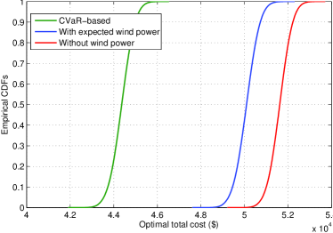
Figure 5: Empirical CDFs of the optimal social cost.

TABLE III: Mean and standard deviation of the total cost and the conventional generation cost: Risk-limiting versus no risk-limiting dispatch. The units are all in $.

Dispatch scheme	Mean	Std	Conv. gen. cost
CVaR-based risk-limiting	44363.26	493.15	26047.66
With expected wind power	50095.68	498.13	50194.59
Without wind power	51619.24	476.25	57122.82

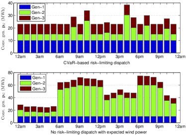
Figure 6: Optimal power dispatch of $\mathbf{p}_{G}$.

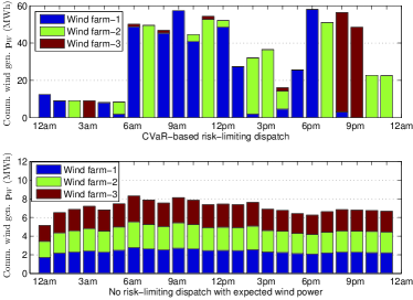
Figure 7: Optimal power dispatch of $\mathbf{p}_{W}$.

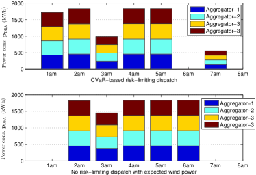
Figure 8: Optimal power dispatch of $\mathbf{p}_{\mathrm{DRA}}$.

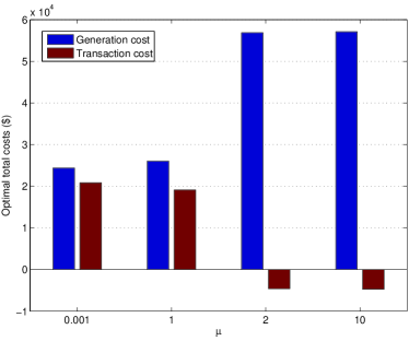
Figure 9: Optimal costs of conventional generation and CVaR-based transaction.

Figure 4 demonstrates the fast convergence of the proposed ADMM-based solver. The pertinent parameters were set to $\rho=35$ and $\lambda^{t}_{j}(0)=p_{jrs}^{t}(0)=0$. Clearly, both the cost and the primal residual converge very fast to the optimum within $10$ iterations. Note that due to the infeasibility of the iterates at the beginning, the objective function starts from a value smaller than the optimum, and then monotonically converge to the latter.

Three methods were tested to show the performance of the optimal dispatch and cost: (i) the novel CVaR-based risk-limiting MC; (ii) the no risk-limiting MC with the expected wind power generation $\{\bar{\mathbf{w}}^{t}\}$; and (iii) the MC without wind power integration. Specifically, $\mathbf{p}^{t}_{W}=\bar{\mathbf{w}}^{t}$ was simply used in the nodal balance (21b) for (ii), while $\mathbf{p}^{t}_{W}\equiv\mathbf{0}$ for (iii). There are no CVaR-pertinent terms in the objective and constraints for the last two alternatives. For all three approaches, the generation cost $\sum_{t=1}^{T}\sum_{i=1}^{N_{g}}C_{i}(P_{G_{i}}^{t})$ is fixed after solving (16). Hence, randomness of the optimal total cost stems from the transaction cost due to the stochasticity of the actual wind power generation $\{\mathbf{w}^{t}\}$ [cf. (11)].

Figure 5 presents the cumulative distribution functions (CDFs) of the optimal total costs using $100,000$ i.i.d. wind samples with mean $\{\bar{\mathbf{w}}^{t}\}$. Clearly, the two competing alternatives always incur higher costs than the novel CVaR-based approach. The values of the mean and standard deviation (std) of the optimal total cost are listed in Table III. It can be seen that, compared with the other two methods, the proposed scheme has a markedly reduced expected total cost and small changes in the std.

Figures 6, 7, and 8 compare the optimal power dispatches $\{\mathbf{p}_{G}^{t},\mathbf{p}_{W}^{t},\mathbf{p}_{\mathrm{DRA}}^{t}\}_{t\in{\cal T}}$ of the proposed scheme with those of the scheme (ii). In Fig. 6, it can be clearly seen that over a single day the CVaR-based MC dispatches lower and smoother $\mathbf{p}_{G}$ than the one with (ii). Furthermore, for the novel method, generators $1$ and $3$ are dispatched to output their minimum generation $P_{G_{i}}^{\min}$, while the output of the generator $2$ changes within its generation limits across time. Such a dispatch results from the economic incentive since the unit $2$ has the lowest generation cost among all three generators [cf. Table I]. On the contrary, both generators $2$ and $3$ fluctuate within a relatively large range in (ii), mainly to meet the variation of base load demand $\mathbf{p}_{BL}$; see Fig. 3.

As shown in Figure 7, the novel CVaR-based approach also dispatches more $\mathbf{p}_{W}^{t}$ than that of (ii). This is because the energy purchase prices $\mathbf{b}^{t}$ are smaller than the conventional generation costs [cf. Table I and Fig. 3]. In addition, $p_{W_{1}}^{t}$ and $p_{W_{2}}^{t}$ contribute most of the committed wind power at $1$pm and $2$pm due to the cheaper buying prices during the corresponding slots [cf. Fig. 3]. Interestingly, Figure 8 shows that the PHEVs are scheduled to start charging earlier for the CVaR-based MC, where $\mathbf{p}_{\mathrm{DRA}}$ is jointly optimized with $\mathbf{p}_{G}$ and $\mathbf{p}_{W}$.

Finally, Figure 9 shows the effect of the weight parameter $\mu$ on the optimal costs of the conventional generation and the CVaR-based transaction. As expected, the CVaR-based transaction cost decreases with the increase of $\mu$. For a larger $\mu$, less $\mathbf{p}_{W}^{t}$ is scheduled so that more wind power is likely to be sold in the RT market that yields selling revenues rather than purchase costs. Consequently, to keep the supply-demand balance, higher conventional generation cost is incurred by the increase of $\mathbf{p}_{G}^{t}$.

VI Conclusions and Future Work

Day-ahead stochastic market clearing with high-penetration wind power was investigated in this paper. A stochastic optimization problem was formulated to minimize the market social cost consisting of the generation cost, the utility of dispatchable loads, as well as the CVaR-based transaction cost. The SAA method was introduced to bypass the inherent high-dimensional integral, while an ADMM-based solver was developed to clear the market in a distributed fashion. Extensive tests on a modified WECC system corroborated the effectiveness of the novel approach, which offers risk-limiting dispatch with considerably reduced conventional generation.

A number of appealing directions open up towards extending the proposed framework. First, it is interesting to study the extended LMPs by solving a large-scale stochastic SCUC with start-up (-down) and no-load costs. Second, a deep explore of the price consistence for multi-period time-coupling MC is in our research agenda. Additional topics worth further investigation include congestion management, reserve procurement, as well as security assessment issues.

Yu Zhang (S’11) received his B.Eng. and M.Sc. degrees (both with highest honors) in Electrical Engineering from Wuhan University of Technology, Wuhan, China, and from Shanghai Jiao Tong University, Shanghai, China, in 2006 and 2010, respectively. Since September 2010, he has been working towards the Ph.D. degree with the Dept. of Electrical and Computer Engineering (ECE) and the Digital Technology Center (DTC) at the University of Minnesota (UMN). During the summer of 2014, he was a research intern with ABB US Corporate Research Center, Raleigh, NC. His research interests span the areas of smart grids, cyber-physical systems, optimization theory, and machine learning. Mr. Zhang received the Huawei Scholarship and the Infineon Scholarship from the Shanghai Jiao Tong University (2009), the ECE Dept. Fellowship from the University of Minnesota (2010), and the Student Travel Awards from the SIAM and the IEEE Signal Processing Society (2014).

Georgios B. Giannakis (F’97) received his Diploma in Electrical Engr. from the Ntl. Tech. Univ. of Athens, Greece, 1981. From 1982 to 1986 he was with the Univ. of Southern California (USC), where he received his MSc. in Electrical Engineering, 1983, M.Sc. in Mathematics, 1986, and Ph.D. in Electrical Engr., 1986. Since 1999 he has been a professor with the Univ. of Minnesota, where he now holds an ADC Chair in Wireless Telecommunications in the ECE Department, and serves as director of the Digital Technology Center. His general interests span the areas of communications, networking and statistical signal processing - subjects on which he has published more than 375 journal papers, 635 conference papers, 21 book chapters, two edited books and two research monographs (h-index 112). Current research focuses on sparsity and big data analytics, wireless cognitive radios, mobile ad hoc networks, renewable energy, power grid, gene-regulatory, and social networks. He is the (co-) inventor of 23 patents issued, and the (co-) recipient of 8 best paper awards from the IEEE Signal Processing (SP) and Communications Societies, including the G. Marconi Prize Paper Award in Wireless Communications. He also received Technical Achievement Awards from the SP Society (2000), from EURASIP (2005), a Young Faculty Teaching Award, the G. W. Taylor Award for Distinguished Research from the University of Minnesota, and the IEEE Fourier Technical Field Award (2014). He is a Fellow of EURASIP, and has served the IEEE in a number of posts, including that of a Distinguished Lecturer for the IEEE-SP Society.

References

- [1] GWEC, “Global wind statistics 2013,” May 2014, [Online]. Available: http://www.gwec.net/wp-content/uploads/2014/02/GWEC-PRstats-2013_EN.pdf.
- [2] “20% wind energy by 2030: Increasing wind energy’s contribution to U.S. electricity supply,” Jul. 2008, [Online]. Available: http://www1.eere.energy.gov/wind/pdfs/41869.pdf.
- [3] “EU energy policy to 2050 – achieving 80-95% emissions reductions,” European Wind Energy Association, Tech. Rep., Mar. 2011.
- [4] X. Liu and W. Xu, “Economic load dispatch constrained by wind power availability: A here-and-now approach,” IEEE Trans. Sustain. Energy, vol. 1, no. 1, pp. 2–9, Apr. 2010.
- [5] Y. Zhang, N. Gatsis, and G. B. Giannakis, “Risk-constrained energy management with multiple wind farms,” in Proc. of Innovative Smart Grid Tech., Washington, D.C., Feb. 2013.
- [6] Q. Fang, Y. Guan, and J. Wang, “A chance-constrained two-stage stochastic program for unit commitment with uncertain wind power output,” IEEE Trans. Power Syst., vol. 27, no. 1, pp. 206–215, 2012.
- [7] E. Sjödin, D. F. Gayme, and U. Topcu, “Risk-mitigated optimal power flow for wind powered grids,” in Proc. of American Control Conf., Montréal, Canada, Jun. 2012, pp. 4431–4437.
- [8] D. Bienstock, M. Chertkov, and S. Harnett, “Chance constrained optimal power flow: Risk-aware network control under uncertainty,” Feb. 2013, [Online]. Avaialble: http://arxiv.org/pdf/1209.5779.pdf.
- [9] R. Rajagopal, E. Bitar, P. Varaiya, and F. Wu, “Risk-limiting dispatch for integrating renewable power,” Intl. J. Elec. Power and energy syst., vol. 44, no. 1, pp. 615–628, Jan. 2013.
- [10] A. Papavasiliou and S. Oren, “Supplying renewable energy to deferrable loads: Algorithms and economic analysis,” in Proc. of IEEE PES General Meeting, Minneapolis, MN, Jul. 2010.
- [11] J. Hetzer, C. Yu, and K. Bhattarai, “An economic dispatch model incorporating wind power,” IEEE Trans. Energy Convers., vol. 23, no. 2, pp. 603–611, Jun. 2008.
- [12] Y. Zhang, N. Gatsis, and G. B. Giannakis, “Robust energy management for microgrids with high-penetration renewables,” IEEE Trans. Sustain. Energy, vol. 4, no. 4, pp. 944–953, Oct. 2013.
- [13] L. Xie, Y. Gu, X. Zhu, and M. G. Genton, “Power system economic dispatch with spatio-temporal wind forecasts,” in Proc. of IEEE EnergyTech, Cleveland, OH, May 2011.
- [14] M. Shahidehpour, H. Yamin, and Z. Li, Market Operations in Electric Power Systems. New York, NY: John Wiley, 2002.
- [15] C. A. Canizares and S. Kodsi, “Power system security in market clearing and dispatch mechanisms,” in Proc. of IEEE PES General Meeting, Montreal, Canada, Jun. 2006.
- [16] E. Hasan, F. D. Galiana, and A. J. Conejo, “Electricity markets cleared by merit order – Part I: Finding the market outcomes supported by pure strategy Nash equilibria,” IEEE Trans. Power Syst., vol. 23, no. 2, pp. 361–371, May 2008.
- [17] N. Gatsis and G. B. Giannakis, “Decomposition algorithms for market clearing with large-scale demand response,” IEEE Trans. Smart Grid, vol. 4, no. 4, pp. 1976–1987, Dec. 2013.
- [18] A. Botterud, Z. Zhou, J. Wang, R. J. Bessa, H. Keko, J. Sumaili, and V. Miranda, “Wind power trading under uncertainty in LMP markets,” IEEE Trans. Power Syst., vol. 27, no. 2, pp. 894–903, May 2012.
- [19] E. Bitar, R. Rajagopal, P. P. Khargonekar, K. Poolla, and P. Varaiya, “Bringing wind energy to market,” IEEE Trans. Power Syst., vol. 27, no. 3, pp. 1225–1235, Aug. 2012.
- [20] J. M. Morales, A. J. Conejo, and J. Pérez-Ruiz, “Short-term trading for a wind power producer,” IEEE Trans. Power Syst., vol. 25, no. 1, pp. 554–564, Feb. 2010.
- [21] G. N. Bathurst, J. Weatherhill, and G. Strbac, “Trading wind generation in short term energy markets,” IEEE Trans. Power Syst., vol. 17, no. 3, pp. 782–789, Aug. 2002.
- [22] A. J. Conejo, M. Carrión, and J. M. Morales, Decision Making Under Uncertainty in Electricity Markets. New York, Dordrecht, Heidelberg, London: Springer, 2010.
- [23] F. Bouffard, F. D. Galiana, and A. J. Conejo, “Market-clearing with stochastic security – Part I: Formulation,” IEEE Trans. Power Syst., vol. 20, no. 4, pp. 1818–1826, Nov. 2005.
- [24] J. M. Morales, A. J. Conejo, K. Liu, and J. Zhong, “Pricing electricity in pools with wind producers,” IEEE Trans. Power Syst., vol. 27, no. 3, pp. 1366–1376, Aug. 2012.
- [25] G. Pritchard, G. Zakeri, and A. Philpott, “A single-settlement, energy-only electric power market for unpredictable and intermittent participants,” Oper. Res., vol. 58, no. 4, pp. 1210–1219, Jul. 2010.
- [26] N. Amjady, J. Aghaei, and H. A. Shayanfar, “Stochastic multiobjective market clearing of joint energy and reserves auctions ensuring power system security,” IEEE Trans. Power Syst., vol. 24, no. 4, pp. 1841–1854, Nov. 2009.
- [27] N. Amjady, A. A. Rashidi, and H. Zareipour, “Stochastic security-constrained joint market clearing for energy and reserves auctions considering uncertainties of wind power producers and unreliable equipment,” Int. Trans. Electr. Energ. Syst., vol. 23, pp. 451–472, May 2013.
- [28] J. M. Morales, M. Zugno, S. Pineda, and P. Pinson, “Electricity market clearing with improved scheduling of stochastic production,” Eur. J. Oper. Res., vol. 235, no. 3, pp. 765–774, Jun. 2014.
- [29] ——, “Redefining the merit order of stochastic generation in forward markets,” IEEE Trans. Power Syst., vol. 29, no. 2, pp. 992–993, Mar. 2014.
- [30] R. T. Rockafellar and S. Uryasev, “Optimization of conditional value-at-risk,” J. Risk, vol. 2, no. 3, pp. 21–41, 2000.
- [31] ——, “Conditional value-at-risk for general loss distributions,” J. of Banking Finance, vol. 26, pp. 1443–1471, 2002.
- [32] F. J. Fabozzi, P. N. Kolm, D. A. Pachamanova, and S. M. Focardi, Robust Portfolio Optimization and Management. Hoboken, NJ: Wiley, 2007.
- [33] A. Botterud, J. Wang, C. Monteiro, and V. Miranda, “Wind power forecasting and electricity market operations,” in Proc. of IAEE Intl. Conf., San Francisco, CA, Jun. 2009.
- [34] J. Rogers and K. Porter, “Wind power and electricity markets,” Oct. 2011, [Online]. Available: http://variablegen.org/wp-content/uploads/2012/11/windinmarketstableOct2011.pdf.
- [35] A. Botterud, Z. Zhou, J. Wang, R. Bessa, H. Keko, J. Mendes, J. Sumaili, and V. Miranda, “Use of wind power forecasting in operational decisions,” Argonne National Laboratory, Tech. Rep., Sep. 2011, [Online]. Available: http://www.dis.anl.gov/pubs/71389.pdf.
- [36] S. Boyd and L. Vandenberghe, Convex Optimization. Cambridge University Press, 2004.
- [37] S. Stoft, Power System Economics: Designing Markets for Electricity. New York, NY: Wiley-IEEE Press, 2002.
- [38] P. Ranci and G. Cervigni, The Economics of Electricity Markets: Theory and Policy. Northampton, MA: Edward Elgar Publishing, 2013.
- [39] F. Paganini, P. Belzarena, and P. Monzón, “Decision making in forward power markets with supply and demand uncertainty,” in Proc. of Conf. Info. Sci. and Syst., Princeton, NJ, Mar. 2014.
- [40] P. W. Sauer and M. A. Pai, Power System Dynamics and Stability. Upper Saddle River, NJ: Prentice Hall, 1998.
- [41] P. R. Gribik, W. W. Hogan, and S. L. Pope, “Market-clearing electricity prices and energy uplift,” Tech. Rep., Dec. 2007, [Online]. Available: http://www.hks.harvard.edu/fs/whogan/Gribik_Hogan_Pope_Price_Uplift_123107.pdf.
- [42] A. J. Kleywegt, A. Shapiro, and T. Homem-De-Mello, “The sample average approximation method for stochastic discrete optimization,” SIAM J. Optim., vol. 12, no. 2, pp. 479–502, 2001.
- [43] T.-H. Chang, M. Alizadeh, and A. Scaglione, “Coordinated home energy management for real-time power balancing,” in Proc. of IEEE PES General Meeting, San Diego, CA, Jul. 2012.
- [44] S.-J. Kim and G. B. Giannakis, “Scalable and robust demand response with mixed-integer constraints,” IEEE Trans. Smart Grid, vol. 4, no. 4, pp. 2089–2099, Dec. 2013.
- [45] S. Boyd, N. Parikh, E. Chu, B. Peleato, and J. Eckstein, “Distributed optimization and statistical learning via the alternating direction method of multipliers,” Found. Trends Mach. Learning, vol. 3, no. 1, pp. 1–122, 2010.
- [46] M. Kraning, E. Chu, J. Lavaei, and S. Boyd, “Dynamic network energy management via proximal message passing,” Found. Trends Optim., vol. 1, no. 2, pp. 70–122, Jan. 2014.
- [47] “Assessment of demand response and advanced metering,” Federal Energy Regulatory Commission, Tech. Rep., Dec. 2012, [Online]. Available: http://www.ferc.gov/legal/staff-reports/12-20-12-demand-response.pdf.
- [48] Y. Zhang, N. Gatsis, and G. B. Giannakis, “Disaggregated bundle methods for distributed market clearing in power networks,” in Proc. of Global Conf. on Signal and Info. Process., Austin, TX, Dec. 2013.
- [49] V. Zavala, M. Anitescu, and J. Birge, “A stochastic electricity market clearing formulation with consistent pricing properties,” Oper. Res. (submitted) 2014, [Online]. Available: http://www.mcs.anl.gov/~anitescu/PUBLICATIONS/2014/zavala-stochpricing-2014.pdf.
- [50] CVX Research Inc., “CVX: Matlab software for disciplined convex programming, version 2.0 (beta),” http://cvxr.com/cvx, Sep. 2012.
- [51] J. F. Sturm, “Using SeDuMi 1.02, a MATLAB toolbox for optimization over symmetric cones,” Optim. Meth. Softw., vol. 11–12, pp. 625–653, Aug. 1999.
- [52] MISO Market Data, [Online]. Available: https://www.misoenergy.org/MarketsOperations/Pages/MarketsOperations.aspx.