A Variable Fixing Heuristic with Local Branching for the Fixed Charge Uncapacitated Network Design Problem with User-optimal Flow

Abstract

This paper presents an iterated local search for the fixed-charge uncapacitated network design problem with user-optimal flow (FCNDP-UOF), which concerns routing multiple commodities from its origin to its destination by designing a network through selecting arcs, with an objective of minimizing the sum of the fixed costs of the selected arcs plus the sum of variable costs associated to the flows on each arc. Besides that, since the FCNDP-UOF is a bilevel problem, each commodity has to be transported through a shortest path, concerning the edges length, in the built network. The proposed algorithm generate a initial solution using a variable fixing heuristic. Then a local branching strategy is applied to improve the quality of the solution. At last, an efficient perturbation strategy is presented to perform cycle-based moves to explore different parts of the solution space. Computational experiments shows that the proposed solution method consistently produces high-quality solutions in reasonable computational times.

1 INTRODUCTION

Due to the continuous development of society, increasing quantities of commodities have to be transported in large urban centers. Therefore, network design problems arise as tools to support decision-making, aiming to meet the need of finding efficient ways to perform the transportation of each commodity from its origin to its destination. In the Fixed Charge Network Design Problem (FCNDP), a subset of edges is selected from a graph, in such a way that a given set of commodities can be transported from their origins to their destinations. The main objective is to minimize the sum of the fixed costs (due to selected edges) and variable costs (depending on the flow of goods on the edges). In addition, fixed and variable costs can be represented by linear functions and arcs are not capacitated. Belonging to a large class of network design problems, the FCNDP has several variations such as shortest path problem, minimum spanning tree problem, vehicle routing problem, traveling salesman problem and Steiner problem in graph [24]. For generic network design problem, such as FCNDP, numerous applications can be found [7, 8, 25], thus, mathematical formulations for the problem may also represent several other problems, like problems of communication, transportation, sewage systems and resource planning. It also appears in other contexts, such as flexible production systems [20] and automated manufacturing systems [15]. Finally, network design problems arise in many vehicle fleet applications that do not involve the construction of physical facilities, but rather model decision problems such as sending a vehicle through a road or not [23, 28].
This work addresses a specific variation of FCNDP, called Fixed-Charge Uncapacitated Network Design Problem with User-optimal Flows (FCNDP-UOF), which consists of adding multiple shortest path problems to the original problem. The FCNDP-UOF involves two distinct agents acting simultaneously rather than sequentially when making decisions. On the upper level, the leader ($1^{st}$ agent) is in charge of choosing a subset of edges to be opened in order to minimize the sum of fixed and variable costs. In response, on the lower level, the follower ($2^{nd}$ agent) must choose a set of shortest paths in the network, through which each commodity will be sent. The effect of an agent on the other is indirect: the decision of the follower is affected by the network designed on the upper level, while the leader’s decision is affected by variable costs imposed by the routes settled in the lower level. The inclusion of shortest path problem constraints in a mixed integer linear programming is not straightforward. Difficulties arise both in modeling and designing efficient methods.
The FCNDP-UOF problem appears in the design of a network for hazardous materials transportation [3, 11, 12, 19]. Particularly for this kind of problem, the government defines a selection of road segments to be opened/closed to the transportation of hazardous materials assuming that the shipments in the resulting network will be done along shortest paths. In hazardous materials transportation problems, roads selected to compose the network have no costs, but the goverment wants to minimize the population exposure in case of an incident during a dangerous-goods transportation. This is a particular case of the FCNDP-UOF problem where, from a mathematical point of view, the fixed costs are equal to zero.
Several variants of the FCNDP-UOF can be seen on [3, 6, 11, 12, 14, 19, 26] and have been treated as part of larger problems in some applications on [17]. The work presented by Bilheimer and Grey [6] formally defines the FCNDP-UOF. Both Erkut et al. [12] and Kara et al. [19] work focus on exact methods, presenting a mathematical formulation and several metrics for the hazardous materials transportation problem. At Mauttone et al. [26], not only was presented a different model, but also a Tabu Search for the FCNDP-UOF. Both, Amaldi et al. [3] and Erkut et al. [11] presented heuristic approaches to deal with the hazardous materials transportation problem. At last, Gonzalez et al. [14], presented an extension of the model proposed by Kara and Verter [19] and also a GRASP.
According to [18, 30], the simplest versions of network design problems are $\mathcal{NP}$-hard and even the task of finding feasible solutions (for problems with budget constraint on the fixed cost) is extremely complex [31]. Therefore, heuristics methods are presented as a good alternative in the search for good solutions. Knowing that, this work proposes an Iterated Local Search [21] for the FCNDP-UOF
This text is organized as follows. In Section 2, we start by describing the problem followed by a bi-level and an one-level formulation, presented on [26]. Then in Section 3 we present our solution approach. Section 4 reports on our computational experiments. At last, in Section 5 the conclusion and future works are presented.

2 GENERAL DESCRIPTION OF FCNDP-UOF

In this section we describe the problem and present a bi-level and an one-level formulation for the FCNDP-UOF proposed respectively by [9, 26] for the FCNDP-UOF.
The basic structures to create a network are a set of nodes $V$ that represents the facilities and a set of uncapacitated and undirected edges $E$ representing the connection between installations. Furthermore, the set $K$ is the set of commodities to be transported over the network, and these commodities may represent physical goods as raw material for industry, hazardous material or even people. Each commodity $k\in K$, has a flow to be delivered through a shortest path between its source $o(k)$ and its destination $d(k)$. The formulation presented here works with variants presenting commodities with multiple origins and destinations, and for treating such a case, it is sufficient to consider that for each pair ($o(k),d(k)$), there is a new commodity resulting from the dissociation of one into several commodities.

2.1 Mathematical Formulation

This subsection presents a few definitions in order to make easier the understanding of the problem.
The model for FCNDP-UOF has two types of variables, one for the construction of the network and another representing the flow. Let $y_{ij}$ be a binary variable, we have that $y_{ij}=1$ if the edge $[i,j]$ is chosen as part of the network and $y_{ij}=0$ otherwise. In this case, $x^{k}_{ij}$ denotes the commodity $k$’s flow through the arc $(i,j)$. Although the edges have no direction, they may be referred to as arcs, because each commodity flow is directed. Treating $y=(y_{ij})$ and $x^{k}=(x^{k}_{ij})$, respectively, as vectors of active edge and flow variables, mixed integer programming formulations can be elaborated.

List of Symbols

$V$	Set of nodes.
$E$	Set of admissible edges.
$K$	Set of commodities.
$A^{E}$	Set of arcs obtained by bidirecting the edges in E.
$\mathcal{G}$	Associated graph $G(V,E)$.
$\delta^{+}_{i}$	Set of all arcs leaving node $i$.
$\delta^{-}_{i}$	Set of all arcs arriving at node $i$.
$c_{a}$	Length of the arc $a$.
$e(a)$	Edge $e$ related to the arc $a$.
$o(k)$	Origin node for commodity $k$.
$d(k)$	Destiny node for commodity $k$.
$g^{k}_{ij}$	Variable cost of transporting commodity
	$k$ through the arc $(i,j)\in A^{E}$.
$f_{ij}$	Fixed cost of opening the edge $[i,j]\in E$.
$y_{ij}$	Indicates whether edge $[i,j]$ belongs in the solution.
$x^{k}_{ij}$	Indicates whether commodity $k$ passes through
	the arc $(i,j)$.

2.2 Bi-level Formulation

In FCNDP-UOF, differently from the basic FCNDP, each commodity $k\in K$ has to be transported through a shortest path between its origin $o(k)$ and its destination $d(k)$, forcing the addition of new constraints to the general problem. Besides selecting a subset of $E$ whose sum of fixed and variable costs is minimal (leading problem), in this variation, we also have to garantee the shortest path constraints for each commodity $k\in K$ (follower problem). The FCNDP-UOF belongs to the class of $\mathcal{NP}$-hard problems and can be modeled as a bi-level mixed integer programming problem [9], as follows:

$$\min\quad \displaystyle\sum\limits_{e\in E}f_{e}y_{e}+\sum\limits_{k\in K}\sum\limits_{(i,j)\in A^{E}}g_{ij}^{k}x_{ij}^{k}$$

s.t. $$y_{e}\in\{0,1\}, \forall e\in E,$$ (1)

where $x_{ij}^{k}$ is a solution of the problem:

$$\min\quad \displaystyle\sum\limits_{k\in K}\sum\limits_{{a=(i,j)}\in A^{E}}c_{a}x_{ij}^{k}$$

s.t. $$\displaystyle\sum\limits_{(i,j)\in\delta^{+}(i)}x_{ij}^{k}-\sum\limits_{(i,j)\in\delta^{-}(i)}x_{ji}^{k}=b_{i}^{k}, \forall i\in V,\forall k\in K,$$ (2)

$$x_{ij}^{k}+x_{ji}^{k}\leq y_{e}, \forall e=[i,j]\in E,\forall k\in K,$$ (3)

$$x_{ij}^{k}\geq 0, \forall(i,j)\in A^{E},\forall k\in K.$$ (4)

where:

$$b_{i}^{k}=\displaystyle\qquad\left\{\begin{array}[]{rl}-1&\textrm{if }i=d(k),\\ 1&\textrm{if }i=o(k),\\ 0&\textrm{otherwise.}\\ \end{array}\right.$$ (8)

According to constraints (1)-(4), we can notice that the set of constraints (1) ensures that the vector of variables $y$ assume only binary values. In (2), we have flow conservation constraints. Constraints (3) do not allow flow into arcs whose corresponding edges are closed. Finally, (4) imposes the non-negativity restriction of the vector of variables $x^{k}$. An interesting remark is that solving the follower problem is equivalent to solving $|K|$ shortest path problems independently.

2.3 One-level Formulation

The FCNDP-UOF can be formulated as a one-level integer programming problem replacing the objective function and the constraints defined by (2)-(4) of the follower problem for its optimality conditions [26]. This can be done by applying the fundamental theorem of duality and the complementary slackness theorem [4], as follows:

$$\min\quad \displaystyle\sum\limits_{e\in E}f_{e}y_{e}+\sum\limits_{k\in K}\sum\limits_{(i,j)\in A^{E}}g_{ij}^{k}x_{ij}^{k}$$

s.t. $$\displaystyle\sum\limits_{{(i,j)}\in\delta^{+}(i)}x_{ij}^{k}-\sum\limits_{(i,j)\in\delta^{-}(i)}x_{ji}^{k}=b_{i}^{k}, \forall i\in V,\forall k\in K,$$ (9)

$$x_{ij}^{k}+x_{ji}^{k}\leq y_{e}, \forall e=[i,j]\in E,\forall k\in K,$$ (10)

$$\pi_{i}^{k}-\pi_{j}^{k}-\lambda_{e(a)}^{k}\leq c_{a} \forall a=(i,j)\in A^{E},k\in K,$$ (11)

$$(y_{e}-x_{ij}^{k}-x_{ji}^{k})\lambda_{e}^{k}=0, \forall e=[i,j]\in E,\forall k\in K,$$ (12)

$$(c_{a}-\pi_{i}^{k}+\pi_{j}^{k}+\lambda_{e(a)}^{k})x_{ij}^{k}=0, \forall a=(i,j)\in A^{E},k\in K,$$ (13)

$$\lambda_{e}^{k}\geq 0, \forall e=[i,j]\in E,k\in K,$$ (14)

$$\pi_{i}^{k}\in\mathbb{R}, \forall i\in V,\forall k\in K,$$ (15)

$$x_{ij}^{k}\geq 0, \forall(i,j)\in A^{E},\forall k\in K,$$ (16)

$$y_{e}\in\{0,1\}, \forall e\in E.$$ (17)

where:

$$b_{i}^{k}=\displaystyle\qquad\left\{\begin{array}[]{rl}-1&\textrm{if }i=d(k),\\ 1&\textrm{if }i=o(k),\\ 0&\textrm{otherwise. }\\ \end{array}\right.$$ (21)

A disadvantage of this new formulation is the loss of linearity of the model. To bypass this problem, a Big-M linearization may be used. After it, one can write the model as a one-level mixed integer linear programming problem, as follows:

$$\min\quad \displaystyle\sum\limits_{e\in E}f_{e}y_{e}+\sum\limits_{k\in K}\sum\limits_{(i,j)\in A^{E}}g_{ij}^{k}x_{ij}^{k}$$

s.t. $$\displaystyle\sum\limits_{{(i,j)}\in\delta^{+}(i)}x_{ij}^{k}-\sum\limits_{(i,j)\in\delta^{-}(i)}x_{ji}^{k}=b_{i}^{k}, \forall i\in V,\forall k\in K,$$ (22)

$$x_{ij}^{k}+x_{ji}^{k}\leq y_{e}, \forall e=[i,j]\in E,\forall k\in K$$ (23)

$$\pi_{i}^{k}-\pi_{j}^{k}-\lambda_{e(a)}^{k}\leq c_{a} \forall a=(i,j)\in A^{E},k\in K,$$ (24)

$$\lambda_{e}^{k}+M_{e}y_{e}-M_{e}x_{ij}^{k}-M_{e}x_{ji}^{k}\leq M_{e}, \forall e=[i,j]\in E,\forall k\in K,$$ (25)

$$M_{e(a)}x_{ij}^{k}-\pi_{i}^{k}+\pi_{j}^{k}+\lambda_{e(a)}^{k}\leq M_{e(a)}-c_{a}, \forall a=(i,j)\in A^{E},k\in K,$$ (26)

$$\lambda_{e}^{k}\geq 0, \forall e=[i,j]\in E,k\in K,$$ (27)

$$\pi_{i}^{k}\in\mathbb{R}, \forall i\in V,\forall k\in K,$$ (28)

$$x_{ij}^{k}\in\{0,1\}, \forall(i,j)\in A^{E},\forall k\in K,$$ (29)

$$y_{e}\in\{0,1\}, \forall e\in E.$$ (30)

where:

$$b_{i}^{k}=\displaystyle\qquad\left\{\begin{array}[]{rl}-1&\textrm{if }i=d(k),\\ 1&\textrm{if }i=o(k),\\ 0&\textrm{otherwise. }\\ \end{array}\right.$$ (34)

However, optimality conditions for the problem in the lower level are, in fact, the optimality conditions of the shortest path problem and they could be expressed in a more compact and efficient way if we consider Bellman’s optimality conditions for the shortest path problem [1] and using a simple lifting process [22].

$$\min\quad \displaystyle\sum\limits_{e\in E}f_{e}y_{e}+\sum\limits_{k\in K}\sum\limits_{(i,j)\in A^{E}}g_{ij}^{k}x_{ij}^{k}$$

s.t. $$\displaystyle\sum\limits_{{(i,j)}\in\delta^{+}(i)}x_{ij}^{k}-\sum\limits_{(i,j)\in\delta^{-}(i)}x_{ji}^{k}=b_{i}^{k}, \forall i\in V,\forall k\in K,$$ (35)

$$x_{ij}^{k}+x_{ji}^{k}\leq y_{ij}, \forall e=[i,j]\in E,\forall k\in K,$$ (36)

$$\pi_{i}^{k}-\pi_{j}^{k}\leq M_{e(a)}-y_{e(a)}(M_{e(a)}-c_{a})-2c_{a}x_{ji}^{k}, \forall a=(i,j)\in A^{E},k\in K,$$ (37)

$$\pi_{d(k)}^{k}=0, \forall k\in K,$$ (38)

$$\pi_{i}^{k}\geq 0, \forall i\in\setminus\{d(k)\},\forall k\in K,$$ (39)

$$x_{ij}^{k}\in\{0,1\}, \forall(i,j)\in A^{E},\forall k\in K,$$ (40)

$$y_{e}\in\{0,1\}, \forall e\in E.$$ (41)

where:

$$b_{i}^{k}=\displaystyle\qquad\left\{\begin{array}[]{rl}-1&\textrm{if }i=d(k),\\ 1&\textrm{if }i=o(k),\\ 0&\textrm{otherwise. }\\ \end{array}\right.$$ (45)

The variables $\pi_{i}^{k}$, $k\in K$, $i\in V$, represent the shortest distance between vertex $i$ and vertex $d(k)$. Then we define that $\pi_{d(k)}^{k}$ will always be equal zero. Assuming that constraints (36), (40) and (41) are satisfied, it is easy to see that constraints (37) are equivalent to Bellman’s optimality conditions for $|K|$ pairs $(o(k),d(k))$.

3 SOLUTION APPROACH

This section focuses on presenting the different methods developed in this work. First the Partial Decoupling Heuristic is introduced. Secondly a procedure to find a lower bound. After that a variable fixing heuristic that uses the previously explained methods. At last a Local Branching (used as Local Search) and a Ejection Cycle (used as Pertubation) are shown so a Iterated Local Search metaheuristics could be done.

3.1 Partial Decoupling Heuristic

The main idea of total decoupling heuristic for the FCNDP-UOF is dissociating the problem of building a network from the shortest path problem. This disintegration, as discussed in [11], can provide worst results than when addressing both problems simultaneously. To work around this situation, the method uses what we call partial decoupling, where certain aspects of the follower problem are considered when trying to build a solution to the leading problem.
The Partial Decoupling Heuristic iterativily builds a network and then routes each commodity so a feasible solution can be built. In order to build the network the cost $\bar{f}_{e}^{k},\mbox{ }e\in E,\mbox{ }k\in K$ is defined:

$$\bar{f}_{e}^{k}=\left\{\begin{array}[]{ll}f_{e}+\alpha\times g^{k}_{ij}+(1-\alpha)\times c_{e}&\quad\text{if $y_{e}=0$,}\\ \alpha\times g^{k}_{ij}+(1-\alpha)\times c_{e}&\quad\text{otherwise.}\\ \end{array}\right.$$ (46)

Doing that we consider whether the edge is open or not, plus a linear combination of the variable cost and the length of the edge as the fixed cost. The $\alpha$ works as a scaling parameter of the importance of the $g^{k}_{ij}$ and $c_{e}$ values. In the beginning of the heuristic $\alpha$ prioritizes the variable cost ($g^{k}_{ij}$), while in the end it prioritizes the edge length ($c_{e}$). It is important to pay attention that $g_{ij}^{k}=q^{k}\beta_{ij}$, where $q^{k}$ represents the amount of commodity $k$ to be transported and $\beta_{ij}$ represents the shipping cost through the edge $e=(i,j)$.
After building the network, another shortest path algorithm, using the edges length ($c_{e}$) as cost, is applied to take every commodity from its origin $o(k)$ to its destination $d(k)$ in the built network.
In order to put the scaling parameter $\alpha$ in good use, the method repeats $MaxIterDP$ times and at each iteration using a different value for $\alpha$. The proposed algorithm is a small variation of the original Partial Decoupling Heuristic [14]. The procedure is further explained on Algorithm 1.

1

2

3Input : $\gamma$, $K$, $\mathcal{G}$

4 Data: $MinCost\leftarrow\infty$, $\alpha\leftarrow 1$, $y\leftarrow 0$, $x\leftarrow 0$;

5 begin

6       $\bar{K}\leftarrow K$;

7       for $numIterDP\mbox{ in }1\ldots MaxIterDP$ do

8             while $\bar{K}\neq\emptyset$ do

9                   $\hat{K}\leftarrow CandidateList(\bar{K},\gamma)$;

10                   $k^{\prime}\leftarrow Random(\hat{K})$;

11                   $y\leftarrow DijkstraLeader(\bar{f}^{k^{\prime}},k^{\prime}$);

12                   $\bar{K}\leftarrow\bar{K}\backslash\{k^{\prime}\}$;

13                  

14            for $k\in K$ do

15                   $x\leftarrow DijkstraFollower(c,k)$;

16                  

17            $s\leftarrow\langle y,x\rangle$;

18             $CloseEdge(s$);

19             if $Cost(s)<MinCost$ then

20                   $s_{best}\leftarrow s$;

21                   $MinCost\leftarrow Cost(s_{best})$;

22                  

23            $\alpha\leftarrow\alpha-\frac{1}{MaxIterDP}$;

24             $\bar{K}\leftarrow K$, $x\leftarrow 0$, $y\leftarrow 0$;

25            

26      return $s_{best}$

27

Algorithm 1 Partial Decoupling Heuristic

To solve the shortest path problem, the partial decoupling heuristic applies the Dijkstra algorithm. At the $|K|$ runs, the function DijkstraLeader solves the problem of network construction, then, the shortest path problem is solved using the DijkstraFollower function, generating a feasible solution. The notation $s\leftarrow\langle y,x\rangle$ means that the solution $s$ is storing the values of the variables $y$ and $x$ that were just defined by DijkstraLeader and DijkstraFollower. Since the function DijskstraLeader can open edges that at the end do not have flow, we used the function CloseEdge() set $y_{e}=0$ for every $x_{ij}^{k}=0\mbox{, }\forall k\in K$. The $Random()$ function returns a random element from the set passed as a parameter. In order to choose the insertion order of the $|K|$ commodities, a candidate list consisting of a subset of commodities not yet routed, whose amount is greater than or equal to $\gamma\%$ times the largest amount ($q_{k}$) of the commodities not routed is create through the use of the function $CandidateList()$.

3.2 LBound Method

LBound Method is a strategy to probably find a stronger lower bound to the original problem. In order to do that, the method consists in relaxing all variables and at each iteration a subset of $y$ variables are turn into binary variables of the model (35) - (41). The process repeats until $\lceil 0.2|E|\rceil$ iterations are done or an integer solution has been found. The number of iterations was decided after numerical experiments. Details of the method could be seen in Algorithm 2:

1 Input : $K$, $\mathcal{G}$

2 Data: $nvbin,cont\leftarrow 0$

3 begin

4       $s_{inf}\leftarrow LinearRelaxion()$;

5       $\bar{E}\leftarrow E$;

6       repeat

7             for $e\in\bar{E}$ do

8                   if $y_{e}\geq 0.5$ then

9                         $y_{e}\in\{0,1\}$;

10                         $\bar{E}\setminus\{e\}$;

11                         $nvbin\leftarrow nvbin+1$;

12                        

13            $s_{inf}\leftarrow SolveR()$;

14            

15            $cont\leftarrow cont+1$;

16            

17      until $cont\geq\lceil 0.2|E|\rceil$ or $OptFound(s_{inf})=TRUE$ or $nvbin>0.9|E|$;

18      return $s_{inf}$

Algorithm 2 LBound

The function $LinearRelaxation()$ solves the linear relaxation of the problem and returns the solution value. The function $SolveR()$ solves a relaxation the problem with a subset of binary variables. Function $OptFound()$ verifies if the solution found by the method is integer or not. It is important to remark that the condition $nvbin>0.9|E|$ was never reached.

3.3 Variable Fixing Heuristic

The Variable Fixing Heuristic (VFH) start using both the Partial Decoupling Heuristic and the LBound method. After applying those two methods, the VHF uses a relax and fix strategy to try to find a better solution. Based on the Relax and Fix Heuristic [29], in this third part, we separate the variables in two distinct sets. $N_{1}$ is the set of relaxed variables and $N_{2}$ is the set of binary variables. Initialy $N_{1}$ contains all variables, while $N_{2}$ is empty. The main idea is at each iteration move a subset of the flow variables ($x^{k}$) from $N_{1}$ to $N_{2}$. At the end of each iteration, if a feasible solution for the relaxed model was found, the variables $y$ that are both zero and attend to the reduced cost criterion for variable fixing, are fixed as zero. The method repeats until all $x^{k}$ have been moved from $N_{1}$ to $N_{2}$ or the duality gap becomes lower than one.
In order to choose the order of $x^{k}$ variables to become binary, the procedure uses a candidate list. To choose a commodity, an element is randomly selected from a candidate list consisting of the commodities whose amount to be transported are greater than or equal to $\gamma\%$ times the largest amount of the commodity whose variables are not set as binary. A pseudo-code of the method is presented in Algorithm 3.

1 Input : $\gamma$, $K$, $\mathcal{G}$

2 Data: $MinCost\leftarrow\infty$

3

4begin

5       $s_{best}\leftarrow\mbox{PartialDecoupling}(\gamma,K,\mathcal{G})$;

6       $s_{inf}\leftarrow LBound(K,\mathcal{G})$;

7       $MinCost\leftarrow Cost(s_{best})$ ;

8       $\bar{K}\leftarrow K$;

9       if $OptFound(s_{inf})\neq TRUE$ then

10             while $\bar{K}\not=\emptyset$ and $|s_{best}-s_{inf}|\geq 1$  do

11                   $k\leftarrow CandidateList(\bar{K},\gamma)$;

12                   $x^{k}\in\{0,1\}$;

13                  

14                  $s\leftarrow SolveR(MinCost)$;

15                   if A feasible solution for the relaxed model was found then

16                         for $e\in E$ do

17                               if $y_{e}=0$ and $RCVF(y_{e})=TRUE$ then

18                                     $y_{e}\leftarrow 0$;

19                                    

20                        if $Cost(s)<MinCost$ and $Feas(s)=TRUE$ then

21                               $s_{best}\leftarrow s$ ;

22                               $MinCost\leftarrow Cost(s_{best})$ ;

23                              

24                        else if $Cost(s)>Cost(s_{inf})$ and $Feas(s)=FALSE$ then

25                               $s_{inf}\leftarrow s$;

26                              

27                  else

28                        Exit

29                  $\bar{K}\leftarrow\bar{K}\setminus\{k\}$

30            return $s_{best}$

31      else

32            return $s_{inf}$

Algorithm 3 VFH

The function $SolveR()$ solves a relaxation of the one level formulation (35)-(41) with a subset of binary variables, taking into consideration the primal bound $MinCost$. $MinCost$ is defined as the current best solution cost. The $RCVF()$ function returns TRUE if the Linear Relaxation cost plus the Reduced Cost of $y_{e}$ is greater than the current VFH solution. The function $Feas()$ returns true if the solution $s$ passed as parameter is a feasible solution to the original problem and returns false otherwise.

3.4 Local Branching

Introduced by Fiscetti and Lodi [13], the Local Branching (LB) technique could be used as a way of improving a given feasible solution. The LB makes use of a MIP solver to explore the solution subspaces effectively. The procedure can be seen as local search, but the neighborhoods are obtained through the introduction of linear inequalities in the MIP model, called local branching cuts. More specifically, the LB searches for a local optimum by restricting the number of variables, from the feasible solution, whose values can be changed.
Formally speaking, consider a feasible solution of the FCNDP-UOP, $s=\langle\bar{y},\bar{x}\rangle\in P$, where $P$ is the polyhedron formed by (35)-(41). The general idea would be adding the LB constraint

$$\sum\limits_{e\in E|\bar{y}_{e}=0}y_{e}+\sum\limits_{e\in E|\bar{y}_{e}=1}(1-y_{e})\leq\Delta,$$ (47)

where $\Delta$ is a given positive integer parameter, indicating the number of variables $y_{e}$, $e\in E$, that are allowed to flip from one to zero and vice versa.
The strategy used here consists on applying the LB constraint only on $y$ variables, leaving $x^{k}$ variables free of LB constraints.

3.5 Ejection Cycle

To understand the principles below the pertubation presented here, it is necessary to get to know a few metrics, developed by [27], to evaluate chains in a solution.
Consider a solution defined by the variables $x_{ij}^{k}$ for each arc $a\in A^{E}$ and each commodity $k\in K$ and $y_{e}$ for each edge $e\in E$. For each open edge $e$, where $y_{e}=1$ and $x_{ij}^{k}>0$ or $x_{ji}^{k}>0$ for at least one commodity $k$, the edge inefficiency ratio can be defined as:

$$I_{e}=\frac{\displaystyle\sum_{k\in K}g_{ij}(x_{ij}^{k}+x_{ji}^{k})+f_{e}}{\displaystyle\sum_{k\in K}(x_{ij}^{k}+x_{ji}^{k})};\qquad\forall e=[i,j]\in E.$$ (48)

The lower the value of $I_{e}$, more interesting it is to have edge $e$ in the solution. The average inefficiency ratio is defined as:

$$\bar{I}=\frac{\displaystyle\sum_{e\in E}I_{e}y_{e}}{\displaystyle\sum_{e\in E}y_{e}}.$$ (49)

With these metrics we can define a set of inefficient edges as:

$$A_{I}=\{e\mbox{ }|\mbox{ }y_{e}=1,I_{e}>\bar{I}\}.$$ (50)

As it can be seen above, the set of inefficient edges contains every edge in the solution whose inefficiency ratio is greater than the average inefficiency ratio. Our aim is to create a movement that remove flows from some of the inefficient edges in set $A_{I}$.
After evaluating the edges it is possible to construct inefficient chains from a subset of the inefficient edges. First, an edge is randomly chosen from the set $A_{I}$ of inefficient edges to form a component of the inefficient chain. If the current partial inefficient chain extends from node i to node j, then an edge $(a,i)\in A_{I}$ or $(j,b)\in A_{I}$ is added to the current chain, where nodes $a$ and $b$ are not included in the current chain. Whenever an edge is added to a chain, it is deleted from $A_{I}$. The process of extending the current chain continues until no further extension is possible or until the chain is composed by four edges. Unless $A_{I}$ is empty or contains a single arc, the process iterates with a random edge chosen to start a new chain. When the process ends, any chains containing a single edge is deleted. This is done in order to decrease the number of edges affected at each iteration of the method.
After constructing a set of inefficient chains, we define our movement. The movement is defined analyzing each chain in the set of inefficient chains.
The key aspect of our pertubation is the re-routing of flow from edges of the inefficient chain to other edges of the network. First, a list of commodities ($K_{SET}$) that have a positive flow through at least one edge of the randomly selected inefficient chain is formed. After that, the opening cost ($f_{e}$) of each edge in the inefficient chain is set as infinity. After reassigning the costs, every commodity in $K_{SET}$ has its route destroyed and reconstructed by the Partial Decoupling Heuristic taking into account the new opening costs. If a feasible solution is found the method stops, else, another inefficient chain is randomly selected and the process restarts. Algorithm 4 describes our Ejection Cycle procedure.

1 Input : $s$, $\gamma$, $K$, $\mathcal{G}$

2

3begin

4      

5      $\mbox{P}\leftarrow PInefChain(s)$;

6       $\bar{s}\leftarrow\emptyset$ ;

7       while $\mbox{P}\not=\emptyset\mbox{ and }\bar{s}\mbox{ is not feasible}$ do

8             $rchain\leftarrow Random(\mbox{P})$;

9             $P\setminus\{rchain\}$;

10             $K_{SET}\leftarrow SK(s,rchain)$;

11             $\bar{s}\leftarrow\mbox{PartialDecoupling}(\mathcal{G},\gamma,K_{SET})$;

12             if $Cost(\bar{s})\leq Cost(s)$ then

13                   $s\leftarrow\bar{s}$;

14                  

15      return $s$

Algorithm 4 Ejection Cycle

In order to clarify Algorithm 4 it is necessary to define a few things. The function $PInefChain()$ returns the set $A_{I}$ of inefficient chains in a solution $s$. The function $SK()$ returns the commodities that have a positive flow in solution $s$ through at least one arc of the inefficient chain passed as parameter and set the fixed costs of the edges in the $rchain$ as infinity. The function PartialDecoupling() reroutes the commodities in $K_{SET}$. In order to do that the DijkstraLeader is applied for all $k\in K_{SET}$ and DijkstraFollower for all $k\in K$. To account those changes, now the method PartialDecoupling() needs to receive a second parameter which is the set o commodities used in DijkstraLeader.Besides that a partial solution for all $k\in K\setminus K_{SET}$ is also passed as a parameter.

3.6 Iterated Local Search

Developed by Lourenço et al. [21], the Iterated Local Search (ILS) is a metaheuristic that applies a local search method repeatedly to a set of solutions obtained by perturbing previously visited local optimal solutions. The ILS presented here uses as its main components, the VFH, the Local Branching and the Ejection Cycle presented in the previously subsections. The methods are applied in a straightforward way. First we ran the VFH to get a feasible solution and a lower bound. Secondly we try to improve the quality of the previously found solution through applying the Local Branching and the Ejection Cycle. The algorithm is described in Algorithm 5.

1 Input : $\gamma$, $\Delta$, $K$, $\mathcal{G}$

2 begin

3       $s,s_{inf}\leftarrow\mbox{VFH}(\mathcal{G},K,\gamma)$;

4       $s\leftarrow\mbox{LB}(s,\Delta)$;

5       $\mbox{UpdateBest}(s)$;

6       if $|cost(s_{best})-cost(s_{inf})|\geq 1$ then

7             while Stop Criterion=false do

8                   $s\leftarrow\mbox{EjectionCycle}(s,\gamma,K,\mathcal{G})$;

9                   $s\leftarrow\mbox{LB}(s,\Delta)$;

10                   $\mbox{UpdateBest}(s)$;

11                  

12      return $s_{best}$

Algorithm 5 VFHLB

In the VFHLB, the initial solution and the lower bound are generated by the VFH method. Then, the function LB performs the Local Branching as a Local Search and the EjectionCycle performs a perturbation.

4 COMPUTATIONAL RESULTS

In this section we present computational results for the VHFLB presented in the previous section.
The algorithm was coded in Xpress Mosel using FICO Xpress Optimization Suite, on an Intel (R) Core TM i3 - 3250 CPU @ 3.5 GHz computer with 8GB of RAM. Computing times are reported in seconds. In order to test the performance of the presented heuristic, we used networks data obtained from Mauttone, Labbé and Figueiredo [26].
In order to calibrate the algorithms we use $60\%$ of our data so parameters overfitting could be avoided and the following $StopCriterion$, $\gamma$ and $\Delta$ values were tested: $StopCriterion=\{10\mbox{ iterations};50\mbox{ iterations};100\mbox{ iterations}\}$, $\gamma=\{0.75,0.85,0.90\}$ and $\Delta=\{\lceil\frac{|E|}{4}\rceil,\lceil\frac{|E|}{3}\rceil,\lceil\frac{|E|}{2}\rceil\}$.After the tests the parameters were calibrated as: $StopCriterion=10\mbox{ iterations}$, $\gamma=0.85$ and $\Delta=\lceil\frac{|E|}{2}\rceil$.
The data used are grouped according to the number of nodes in the graph (10, 20, 30), followed by the graph density (0.3, 0.5, 0.8) and finally the amount of different commodities to be transported (5, 10, 15, 20, 30, 45).
We are comparing the VFHLB results with the results of the GRASP presented by [14], which, to the best of our knowledge, is the best heuristic aproach to solve the FCNDP-UOF. For the presented tables, we report the best solution (Best Sol) and best time (Best Time) reached by each approach, the average gap (Avg GAP) and the gap (GAP) using the optimal solution. We also reported the average values for time (Avg Time) and for solutions (Avg Sol). Finally, it is reported standard deviation values for time (Dev Time) and solution (Dev Sol). The results in bold represent that the optimum has been found.

	GRASP								VFHLB
	Avg Sol	Avg Time	Dev Sol	Dev Time	Best Sol	Best Time	Avg GAP	GAP	Avg Sol	Avg Time	Dev Time	Best Sol	Best Time	Avg GAP	GAP
10-0.3-5-1	3942.00	1.2870	0.0000	0.0329	3942	1.2561	0.0000	0.0000	3942	0.0070	0.0017	3942	0.0060	0.0000	0.0000
10-0.3-5-2	4552.00	1.3267	0.0000	0.0172	4552	1.3110	0.0000	0.0000	4552	0.0038	0.0004	4552	0.0030	0.0000	0.0000
10-0.3-5-3	5762.00	1.2470	0.0000	0.0276	5762	1.2420	0.0000	0.0000	5762	0.0040	0.0000	5762	0.0040	0.0000	0.0000
10-0.3-5-4	4811.00	1.3150	0.0000	0.0230	4811	1.2834	0.0000	0.0000	4811	0.0044	0.0009	4811	0.0040	0.0000	0.0000
10-0.3-5-5	4831.00	1.3158	0.0000	0.0418	4831	1.3080	0.0000	0.0000	4831	0.0034	0.0005	4831	0.0030	0.0000	0.0000
10-0.3-10-1	8331.00	2.6486	0.0000	0.0462	8331	2.6380	0.0000	0.0000	8331	0.0136	0.0021	8331	0.0120	0.0000	0.0000
10-0.3-10-2	8812.00	2.8110	0.0000	0.0755	8812	2.7941	0.0000	0.0000	8812	0.0128	0.0024	8812	0.0110	0.0000	0.0000
10-0.3-10-3	10016.00	2.7410	0.0000	0.0395	10016	2.7246	0.0000	0.0000	10016	0.0080	0.0007	10016	0.0070	0.0000	0.0000
10-0.3-10-4	8750.00	2.6676	0.0000	0.0804	8750	2.6000	0.0000	0.0000	8750	0.0072	0.0004	8750	0.0070	0.0000	0.0000
10-0.3-10-5	10130.00	2.7004	0.0000	0.0847	10130	2.6950	0.0000	0.0000	10130	0.0186	0.0040	10130	0.0160	0.0000	0.0000
10-0.3-15-1	12490.00	4.1740	0.0000	0.1084	12490	4.1657	0.0000	0.0000	12490	0.0186	0.0036	12490	0.0170	0.0000	0.0000
10-0.3-15-2	17417.00	4.1920	0.0000	0.0762	17417	4.0662	0.0000	0.0000	17417	0.0208	0.0013	17417	0.0200	0.0000	0.0000
10-0.3-15-3	12378.00	4.2074	0.0000	0.1048	12378	4.1990	0.0000	0.0000	12378	0.0182	0.0045	12378	0.0150	0.0000	0.0000
10-0.3-15-4	11007.00	4.2281	0.0000	0.0549	11007	4.1210	0.0017	0.0017	10988	0.0196	0.0029	10988	0.0170	0.0000	0.0000
10-0.3-15-5	9066.00	4.2565	0.0000	0.0537	9066	4.2060	0.0000	0.0000	9066	0.0158	0.0008	9066	0.0150	0.0000	0.0000
20-0.3-10-1	6513.58	15.6530	136.4805	0.3393	6411	15.4965	0.0896	0.0724	5978	0.6980	0.0098	5978	0.6840	0.0000	0.0000
20-0.3-10-2	10813.30	16.5735	185.6884	0.5755	10664	16.3770	0.0329	0.0186	10469	4.7662	0.0886	10469	4.6650	0.0000	0.0000
20-0.3-10-3	7286.40	15.9854	132.1352	0.3434	7200	15.6720	0.0379	0.0256	7020	3.7044	0.1155	7020	3.5470	0.0000	0.0000
20-0.3-10-4	5754.74	15.8370	116.7287	0.3310	5598	15.7103	0.0494	0.0208	5484	2.7238	0.0806	5484	2.6230	0.0000	0.0000
20-0.3-10-5	8322.00	16.0420	0.0000	0.3995	8322	16.0100	0.0492	0.0492	7932	14.4424	0.2933	7932	14.1280	0.0000	0.0000
20-0.3-20-1	9488.00	32.0957	0.0000	1.3602	9488	31.8410	0.0000	0.0000	9488	0.8662	0.0272	9488	0.8400	0.0000	0.0000
20-0.3-20-2	11699.86	31.6390	201.3070	0.9075	11607	30.9429	0.0155	0.0075	11521	3.3546	0.1505	11521	3.2080	0.0000	0.0000
20-0.3-20-3	8670.82	32.5660	222.8998	0.7159	8568	32.4357	0.0485	0.0360	8270	1.2644	0.0393	8270	1.2280	0.0000	0.0000
20-0.3-20-4	12320.58	31.9430	300.0561	1.0738	11985	31.6236	0.0353	0.0071	11901	21.8506	0.9442	11901	21.0000	0.0000	0.0000
20-0.3-20-5	10379.38	32.1230	178.5869	0.4624	10297	31.9303	0.0749	0.0664	9656	1.8926	0.0947	9656	1.8190	0.0000	0.0000
20-0.3-30-1	13244.00	49.2763	0.0000	0.7556	13244	48.6920	0.0587	0.0587	12510	1.4656	0.0292	12510	1.4280	0.0000	0.0000
20-0.3-30-2	14854.90	49.8060	364.8115	1.7615	14737	49.4076	0.0449	0.0366	14216	2.2224	0.1063	14216	2.1130	0.0000	0.0000
20-0.3-30-3	14687.52	48.1790	577.2804	1.4053	14629	47.7936	0.0967	0.0923	13393	5.2596	0.1448	13393	5.0720	0.0000	0.0000
20-0.3-30-4	15420.97	48.6160	327.7683	0.6324	15329	48.3243	0.0670	0.0607	14452	1.7608	0.0733	14452	1.6980	0.0000	0.0000
20-0.3-30-5	12599.00	51.3221	0.0000	1.0764	12599	51.0160	0.1033	0.1033	11419	1.3276	0.0398	11419	1.2950	0.0000	0.0000
30-0.3-15-1	8529.32	69.3908	263.2338	1.5946	8395	68.5680	0.0879	0.0708	7840	2.3482	0.0674	7840	2.2900	0.0000	0.0000
30-0.3-15-2	10051.33	65.7535	340.4006	1.0051	10112	64.7180	0.0604	0.0668	9479	11.9144	0.2141	9479	11.6160	0.0000	0.0000
30-0.3-15-3	7422.75	66.0270	196.0199	1.8967	7281	65.7629	0.0536	0.0335	7045	5.4786	0.0389	7045	5.4180	0.0000	0.0000
30-0.3-15-4	8775.16	66.4171	168.0749	2.3415	8654	65.8900	0.0414	0.0271	8426	26.4730	0.5365	8426	25.7670	0.0000	0.0000
30-0.3-15-5	9626.00	66.1244	0.0000	2.0463	9626	65.7300	0.0949	0.0949	8792	98.2168	1.1438	8792	97.3190	0.0000	0.0000
30-0.3-30-1	15766.28	133.4690	287.2792	2.8935	15286	132.1343	0.1927	0.1564	13219	9.4686	0.0500	13219	9.4110	0.0000	0.0000
30-0.3-30-2	14308.35	138.7550	252.7530	2.3416	13973	137.6450	0.0908	0.0653	13117	35.3648	0.6179	13117	34.8360	0.0000	0.0000
30-0.3-30-3	15504.47	139.7580	580.6050	3.8356	15412	137.8014	0.1450	0.1382	13541	18.5124	0.3369	13541	18.2120	0.0000	0.0000
30-0.3-30-4	14766.19	132.6110	254.0662	2.3091	14649	130.7544	0.1546	0.1454	12789	31.2224	1.5092	12789	29.8950	0.0000	0.0000
30-0.3-30-5	13841.41	133.6140	307.9978	3.7867	13517	133.0795	0.1634	0.1362	11897	8.3360	0.3231	11897	8.0590	0.0000	0.0000
30-0.3-45-1	18885.64	204.8792	663.5134	2.6948	18773	200.8620	0.1849	0.1779	15938	16.7946	0.6475	15938	16.4120	0.0000	0.0000
30-0.3-45-2	14455.60	206.9196	597.8858	4.3356	14200	203.6610	0.0955	0.0761	13196	29.0830	0.5499	13196	28.5450	0.0000	0.0000
30-0.3-45-3	19346.43	202.7890	340.7032	6.4728	18893	202.3834	0.0240	0.0000	18893	230.5346	8.5348	18893	223.8230	0.0000	0.0000
30-0.3-45-4	19162.29	215.2056	637.8094	4.2326	19048	209.7520	0.0870	0.0805	17629	29.6728	0.6131	17629	29.2020	0.0000	0.0000
30-0.3-45-5	17909.32	205.4560	231.1970	6.6092	17732	200.9360	0.0926	0.0817	16392	250.6620	4.4910	16392	246.4560	0.0000	0.0000
Avg	11171.1236	57.2432			11078.3111	56.5236	0.0528	0.0446	10537.2889	19.3746		10537.2889	18.9504	0.0000	0.0000

Table 1: Computational results for GRASP and VFHLB approaches for $0.3$ density instances

	GRASP								VFHLB
	Avg Sol	Avg Time	Dev Sol	Dev Time	Best Sol	Best Time	Avg GAP	GAP	Avg Sol	Avg Time	Dev Time	Best Sol	Best Time	Avg GAP	GAP
10-0.5-5-1	4360.00	1.8240	0.0000	0.0568	4360	1.8058	0.0000	0.0000	4360	0.0086	0.0005	4360	0.0080	0.0000	0.0000
10-0.5-5-2	1351.00	1.9186	0.0000	0.0632	1351	1.9110	0.0000	0.0000	1351	0.0092	0.0004	1351	0.0090	0.0000	0.0000
10-0.5-5-3	2932.00	1.8339	0.0000	0.0533	2932	1.8050	0.0000	0.0000	2932	0.0082	0.0011	2932	0.0070	0.0000	0.0000
10-0.5-5-4	4920.00	1.9230	0.0000	0.0662	4920	1.8890	0.0000	0.0000	4920	0.2516	0.0138	4920	0.2430	0.0000	0.0000
10-0.5-5-5	4469.00	1.8880	0.0000	0.0604	4469	1.8730	0.0000	0.0000	4469	0.0184	0.0009	4469	0.0180	0.0000	0.0000
10-0.5-10-1	7566.00	3.7367	0.0040	0.1192	7566	3.7070	0.0040	0.0040	7536	0.0542	0.0008	7536	0.0530	0.0000	0.0000
10-0.5-10-2	7575.96	3.7589	193.3202	0.0645	7442	3.7070	0.0431	0.0246	7263	0.3026	0.0027	7263	0.3000	0.0000	0.0000
10-0.5-10-3	5399.55	3.7424	131.8461	0.0968	5273	3.6980	0.0240	0.0000	5273	0.0166	0.0005	5273	0.0160	0.0000	0.0000
10-0.5-10-4	5983.61	3.8770	105.7580	0.0847	5901	3.8460	0.0221	0.0080	5854	0.0174	0.0009	5854	0.0170	0.0000	0.0000
10-0.5-10-5	5102.45	3.7687	66.9842	0.0719	5032	3.7240	0.0240	0.0098	4983	0.8284	0.0187	4983	0.8060	0.0000	0.0000
10-0.5-15-1	9379.00	5.6480	0.0041	0.1157	9379	5.5350	0.0041	0.0041	9341	0.0312	0.0013	9341	0.0300	0.0000	0.0000
10-0.5-15-2	7512.00	5.7720	0.0000	0.0759	7512	5.7027	0.1264	0.1264	6669	0.0236	0.0013	6669	0.0220	0.0000	0.0000
10-0.5-15-3	10324.00	5.9603	0.0000	0.1085	10324	5.9130	0.0000	0.0000	10324	0.3338	0.0041	10324	0.3300	0.0000	0.0000
10-0.5-15-4	6339.00	5.9380	0.0000	0.2099	6339	5.8100	0.0000	0.0000	6339	0.0810	0.0025	6339	0.0790	0.0000	0.0000
10-0.5-15-5	9519.00	5.9964	0.0002	0.1417	9519	5.9370	0.0002	0.0002	9517	4.0846	0.0354	9517	4.0300	0.0000	0.0000
20-0.5-10-1	4784.00	21.5620	0.0000	0.8304	4784	21.4326	0.0000	0.0000	4784	2.6538	0.0199	4784	2.6310	0.0000	0.0000
20-0.5-10-2	7689.00	21.8640	0.0000	0.5656	7689	21.7328	0.0000	0.0000	7689	1.9200	0.0466	7689	1.8770	0.0000	0.0000
20-0.5-10-3	6184.00	22.6760	0.0000	0.4702	6184	22.4492	0.0000	0.0000	6184	0.5824	0.0102	6184	0.5670	0.0000	0.0000
20-0.5-10-4	5532.91	22.4149	95.1989	0.2894	5489	22.1930	0.0663	0.0578	5189	1.6642	0.0275	5189	1.6330	0.0000	0.0000
20-0.5-10-5	6233.72	22.7810	80.4730	0.5918	6172	22.7354	0.0302	0.0200	6051	26.7656	0.0977	6051	26.6630	0.0000	0.0000
20-0.5-20-1	9964.00	46.5030	0.0000	0.9544	9964	45.8520	0.1302	0.1302	8816	2.9528	0.0153	8816	2.9320	0.0000	0.0000
20-0.5-20-2	8721.34	47.4527	150.4528	1.8322	8584	46.8900	0.0160	0.0000	8584	4.4280	0.0511	8584	4.3720	0.0000	0.0000
20-0.5-20-3	8354.83	45.7165	214.8412	0.9228	8305	44.6450	0.1051	0.0985	7560	7.0656	0.0300	7560	7.0130	0.0000	0.0000
20-0.5-20-4	7750.74	45.2840	100.0567	0.8360	7674	44.9217	0.0153	0.0052	7634	1.5694	0.0201	7634	1.5470	0.0000	0.0000
20-0.5-20-5	8636.00	44.8590	0.0000	1.1159	8636	44.7693	0.0443	0.0443	8270	6.0790	0.0509	8270	6.0160	0.0000	0.0000
20-0.5-30-1	12600.00	67.9890	0.0000	2.3355	12600	67.9890	0.2406	0.2406	10156	1.8056	0.0785	10156	1.7300	0.0000	0.0000
20-0.5-30-2	12932.00	68.6630	0.0000	1.9053	12932	68.6630	0.1341	0.1341	11403	7.2198	0.2475	11403	7.0420	0.0000	0.0000
20-0.5-30-3	13021.40	73.2877	334.7399	1.3527	12867	71.5700	0.1225	0.1092	11600	13.7846	0.3707	11600	13.5040	0.0000	0.0000
20-0.5-30-4	12333.56	70.8795	317.1527	1.3237	12260	68.8150	0.0465	0.0403	11785	6.8018	0.0628	11785	6.7190	0.0000	0.0000
20-0.5-30-5	10989.00	69.4657	0.0000	1.8168	10989	69.3270	0.1496	0.1496	9559	7.3206	0.0511	9559	7.2530	0.0000	0.0000
30-0.5-15-1	6824.93	104.3949	112.2020	3.3325	6744	103.9790	0.1707	0.1568	5830	12.4814	0.1506	5830	12.3470	0.0000	0.0000
30-0.5-15-2	6888.00	103.6410	0.0000	4.0814	6888	102.8119	0.0527	0.0527	6543	20.0704	0.1470	6543	19.8560	0.0000	0.0000
30-0.5-15-3	5809.89	109.4442	52.8671	2.4582	5741	107.5090	0.0223	0.0102	5683	14.5294	0.1577	5683	14.3380	0.0000	0.0000
30-0.5-15-4	6097.00	106.1190	0.0000	2.2691	6097	103.3599	0.0919	0.0919	5584	11.6152	0.1212	5584	11.4330	0.0000	0.0000
30-0.5-15-5	5794.00	108.9972	0.0000	3.4635	5794	107.9180	0.0000	0.0000	5794	22.8150	1.1958	5794	21.9610	0.0000	0.0000
30-0.5-30-1	8823.02	209.1856	151.8084	6.4735	8753	207.9380	0.0274	0.0192	8588	28.3988	0.5552	8588	27.9600	0.0000	0.0000
30-0.5-30-2	9134.00	212.8090	0.0000	3.6315	9134	211.9578	0.0432	0.0432	8756	56.7008	1.7342	8756	55.3860	0.0000	0.0000
30-0.5-30-3	10908.73	206.0050	138.0897	4.4661	10591	203.9450	0.0300	0.0000	10591	445.2772	13.4245	10591	432.3970	0.0000	0.0000
30-0.5-30-4	9120.14	210.4039	227.4169	6.4708	9012	209.1490	0.1240	0.1107	8114	74.5170	1.2355	8114	73.2920	0.0000	0.0000
30-0.5-30-5	13575.00	214.7650	0.0000	3.1942	13575	209.1811	0.0700	0.0700	12687	117.1688	2.5543	12687	114.8630	0.0000	0.0000
30-0.5-45-1	11160.00	332.1730	0.0000	13.8050	11160	330.1800	0.0953	0.0953	10189	31.7414	0.3404	10189	31.3220	0.0000	0.0000
30-0.5-45-2	12105.07	319.6155	248.6762	7.4214	12009	316.4510	0.1540	0.1448	10490	67.9630	2.6552	10490	65.6430	0.0000	0.0000
30-0.5-45-3	15733.00	324.8540	0.0000	6.0844	15733	315.7581	0.1509	0.1509	13670	150.6902	8.3190	13670	142.3510	0.0000	0.0000
30-0.5-45-4	10910.00	322.2408	0.0000	4.1851	10910	316.5430	0.1321	0.1321	9637	76.2042	2.7176	9637	73.6180	0.0000	0.0000
30-0.5-45-5	12870.05	314.7070	267.3752	5.6402	12593	310.3011	0.1086	0.0848	11609	17.7640	0.4141	11609	17.3510	0.0000	0.0000
Avg	8315.8204	87.7409			8270.7111	86.6185	0.0583	0.0527	7781.3333	27.7027		7781.3333	26.9241	0.0000	0.0000

Table 2: Computational results for GRASP and VFHLB approaches for $0.5$ density instances

	GRASP								VFHLB
	Avg Sol	Avg Time	Dev Sol	Dev Time	Best Sol	Best Time	Avg GAP	GAP	Avg Sol	Avg Time	Dev Time	Best Sol	Best Time	Avg GAP	GAP
10-0.8-5-1	4033.83	3.0370	108.4895	0.0314	3986	3.0249	0.1146	0.1014	3619	0.0142	0.0004	3619	0.0140	0.0000	0.0000
10-0.8-5-2	3535.68	2.9300	60.9944	0.0883	3480	2.9100	0.0160	0.0000	3480	0.1480	0.0016	3480	0.1460	0.0000	0.0000
10-0.8-5-3	3330.27	2.7480	112.2499	0.0442	3317	2.7150	0.1035	0.0991	3018	0.2422	0.0041	3018	0.2380	0.0000	0.0000
10-0.8-5-4	3518.00	2.9770	0.0000	0.0614	3518	2.8758	0.0000	0.0000	3518	0.0886	0.0009	3518	0.0880	0.0000	0.0000
10-0.8-5-5	3960.68	2.7730	80.1635	0.0521	3906	2.7620	0.0232	0.0090	3871	0.0390	0.0012	3871	0.0380	0.0000	0.0000
10-0.8-10-1	6031.84	5.9723	114.2613	0.0866	5902	5.8210	0.0376	0.0153	5813	0.0458	0.0046	5813	0.0430	0.0000	0.0000
10-0.8-10-2	5120.64	5.7880	107.2940	0.1479	5040	5.6954	0.0160	0.0000	5040	1.0682	0.0285	5040	1.0440	0.0000	0.0000
10-0.8-10-3	3975.00	5.9039	0.0000	0.1344	3975	5.8570	0.1360	0.1360	3499	0.0826	0.0018	3499	0.0810	0.0000	0.0000
10-0.8-10-4	5460.55	5.9090	116.8811	0.1723	5364	5.7908	0.0180	0.0000	5364	0.0876	0.0086	5364	0.0830	0.0000	0.0000
10-0.8-10-5	4225.54	5.7690	72.7043	0.1662	4192	5.7690	0.0224	0.0143	4133	1.1376	0.0334	4133	1.0860	0.0000	0.0000
10-0.8-15-1	6976.61	8.9230	90.2083	0.3180	6935	8.8338	0.0227	0.0166	6822	0.1478	0.0040	6822	0.1440	0.0000	0.0000
10-0.8-15-2	5276.29	8.8852	77.3640	0.1640	5183	8.6770	0.0180	0.0000	5183	0.1492	0.0027	5183	0.1450	0.0000	0.0000
10-0.8-15-3	5017.00	9.0300	0.0000	0.0780	5017	8.9940	0.1092	0.1092	4523	0.6238	0.0080	4523	0.6140	0.0000	0.0000
10-0.8-15-4	7663.62	8.9097	64.8997	0.2998	7484	8.8390	0.0240	0.0000	7484	0.6206	0.0086	7484	0.6070	0.0000	0.0000
10-0.8-15-5	4751.60	9.2254	85.5372	0.2468	4686	9.2070	0.2364	0.2194	3843	0.4682	0.0066	3843	0.4610	0.0000	0.0000
20-0.8-10-1	4120.80	34.3230	105.3503	0.8950	4040	34.3230	0.0440	0.0236	3947	0.6520	0.0107	3947	0.6440	0.0000	0.0000
20-0.8-10-2	3915.00	34.5080	0.0000	1.1326	3915	34.0249	0.0460	0.0460	3743	6.9310	0.2826	3743	6.7250	0.0000	0.0000
20-0.8-10-3	3480.24	34.8060	74.7532	0.5791	3412	34.3883	0.0200	0.0000	3412	0.1918	0.0033	3412	0.1880	0.0000	0.0000
20-0.8-10-4	4209.00	35.2740	0.0000	0.8032	4209	34.9940	0.0301	0.0301	4086	5.0812	0.1772	4086	4.9450	0.0000	0.0000
20-0.8-10-5	4542.98	35.6360	97.5143	0.7726	4498	35.2796	0.0100	0.0000	4498	4.6612	0.0678	4498	4.6030	0.0000	0.0000
20-0.8-20-1	6909.00	70.8823	0.0000	1.7308	6909	69.2210	0.1920	0.1920	5796	4.2190	0.0869	5796	4.1280	0.0000	0.0000
20-0.8-20-2	7635.54	71.4810	187.0284	1.0189	7590	70.3373	0.0851	0.0786	7037	313.3302	20.9517	7037	297.9690	0.0000	0.0000
20-0.8-20-3	6251.89	68.9992	89.4775	1.8381	5422	68.1810	0.3603	0.1797	4596	5.2952	0.1021	4596	5.2230	0.0000	0.0000
20-0.8-20-4	5187.00	70.2559	69.0130	2.4494	5250	69.9760	0.0693	0.0823	4851	2.8762	0.0466	4851	2.8170	0.0000	0.0000
20-0.8-20-5	6855.53	72.1322	86.2333	1.9296	6267	71.4180	0.1264	0.0297	6086	10.8284	0.5098	6086	10.5270	0.0000	0.0000
20-0.8-30-1	9425.00	105.0060	0.0000	2.1653	9425	101.2258	0.2132	0.2132	7769	7.7738	0.0747	7769	7.7040	0.0000	0.0000
20-0.8-30-2	8735.33	110.7691	126.4167	1.9805	8666	109.8900	0.1373	0.1282	7681	14.1722	0.2527	7681	13.9840	0.0000	0.0000
20-0.8-30-3	5947.89	107.2994	201.4348	2.6665	5889	106.2370	0.1563	0.1448	5144	14.6920	0.3542	5144	14.4420	0.0000	0.0000
20-0.8-30-4	8768.08	104.7711	177.5349	3.7392	8630	104.5620	0.2198	0.2006	7188	48.2594	2.3096	7188	46.6700	0.0000	0.0000
20-0.8-30-5	8175.16	108.0789	127.8169	1.4551	7942	108.0789	0.1086	0.0770	7374	20.4534	0.6175	7374	19.9750	0.0000	0.0000
30-0.8-15-1	3091.61	171.4778	66.3609	0.7593	3061	169.7800	0.0100	0.0000	3061	4.5098	0.0911	3061	4.4170	0.0000	0.0000
30-0.8-15-2	3506.00	160.2209	0.0000	5.1644	3506	160.2209	0.0139	0.0139	3458	11.7516	0.2655	3458	11.5390	0.0000	0.0000
30-0.8-15-3	5159.56	166.8339	44.5643	2.8985	5139	163.8840	0.0910	0.0867	4729	105.0818	7.0616	4729	100.5670	0.0000	0.0000
30-0.8-15-4	7312.13	160.7620	161.4134	3.4133	7283	159.4759	0.0925	0.0882	6693	53.8938	2.2803	6693	52.1000	0.0000	0.0000
30-0.8-15-5	6263.50	164.5370	113.3484	2.7050	6251	162.5860	0.0455	0.0434	5991	34.2898	1.3369	5991	33.3210	0.0000	0.0000
30-0.8-30-1	4871	332.1400	0.0000	9.2200	4871	330.9080	0.0085	0.0085	4830	27.9676	0.5595	4830	27.3360	0.0000	0.0000
30-0.8-30-2	7122.2	328.2900	182.3900	4.1100	6989	325.3570	0.0191	0.0000	6989	296.6414	21.9387	6989	279.8210	0.0000	0.0000
30-0.8-30-3	8124	337.1900	16.4300	33.6300	8112	321.8380	0.0488	0.0473	7746	2115.6020	49.0532	7746	2074.4600	0.0000	0.0000
30-0.8-30-4	8384	318.0600	0.0000	26.0900	8384	338.2490	0.0000	0.0000	8384	530.1420	15.6519	8384	520.0250	0.0000	0.0000
30-0.8-30-5	7442.8	321.4300	33.0900	17.8900	7428	344.3670	0.0020	0.0000	7428	162.6760	2.9126	7428	159.9620	0.0000	0.0000
30-0.8-45-1	6633.24	495.3080	118.1999	11.4544	6620	494.3174	0.0547	0.0526	6289	48.6748	1.2567	6289	47.7090	0.0000	0.0000
30-0.8-45-2	11150.60	489.6256	220.3763	15.3625	10975	489.6256	0.3142	0.2935	8485	377.5736	13.7328	8485	367.7370	0.0000	0.0000
30-0.8-45-3	9555.00	507.0021	399.7143	17.2257	9555	507.0021	0.2327	0.2327	7751	507.0248	20.1638	7751	495.2200	0.0000	0.0000
30-0.8-45-4	11214.00	492.2408	0.0000	16.3840	11214	489.3050	0.1906	0.1906	9419	2441.1600	31.0341	9419	2414.4100	0.0000	0.0000
30-0.8-45-5	8338.56	528.5251	155.1697	7.6185	8080	522.2580	0.0577	0.0249	7884	134.6612	1.0177	7884	133.4330	0.0000	0.0000
Avg	6115.6400	136.1477			6033.7111	135.9796	0.0866	0.0717	5590.1111	162.5785		5590.1111	159.2763	0.0000	0.0000

Table 3: Computational results for GRASP and VFHLB approaches for $0.8$ density instances

In Tables 1, 2, 3 were used 135 instances generated by Mautonne, Labbé and Figueiredo [26], whose results were published by them just for 5 instances. For these instances, the computational results suggest the efficiency of VFHLB. On average, the time spent by VFHLB was 2.31 times faster than the time spent by GRASP, being 2.954 times faster for 0.3 density networks, 3.167 times for 0.5 density networks and 0.837 times for 0.8 density networks. Also, VFHLB found all optimal solutions, while GRASP found only 44 optimal solutions. Besides that, the VFHLB also improved or equaled GRASP results for all 135 instances (91 improvements and 44 draws).
Another important remark is that, in Tables 1 and 2 VFHLB is faster than GRASP, both in the mean of Avg Times and in the mean of Best Times. Although VFHLB lose to GRASP in the mean of Avg Times and in the mean of Best Times on Table 3. On the other hand, GRASP finds only 26 $\%$ of the optimal solutions while, as told before, VFHLB finds all optimal solutions.
The experiment also showed that, at least for the instances tested, the order of the commodities set by the candidate list in the VFHLB does not change the solution obtained at the end of the algoritm, but does affect the computational time.

4.1 Statistical Analysis

In order to verify whether or not the differences of mean values obtained by the evaluated strategies shown in Tables 1,2 and 3 are statistically significant, we employed the Wilcoxon-Mann-Whitney test technique [16]. This test could be applied to compare algorithms with some random features and identify if the difference of performance between them is due to randomness.
According to [16], this statistical test is used when two independent samples are compared and whenever it is necessary to have a statistical test to reject the null hypothesis, with a significance $\theta$ level (i.e., it is possible to reject the null hypothesis with the probability of ($1-\theta\times 100\%$)). For the sake of this analysis we considered $\theta=0.01$. The hypotheses considered in this test are:

• Null Hypothesis (H0): there are no significant differences between the solutions found by VFHLB and the original method;

• Alternative Hypothesis (H1): there are significant differences (bilateral alternative) between the solutions found by VFHLB and the GRASP.

Table 4 presents the number of better average solutions found by each strategy, for each group of instances separeted by density. The number of cases where the Null Hypothesis was rejected is also shown between parentheses.

Instance	Algorithms
Groups	GRASP	VFHLB
0.3	0(0)	30(29)
0.5	0(0)	34(31)
0.8	0(0)	43(33)

Table 4: Statistical Analysis of GRASP and DPRFLB

When comparing GRASP with VFHLB, we notice that almost all differences of performance ($86.91\%$ of the tests) are statistically significant. We can also observe that the VFHLB obtained $100\%$ of the best results. These results indicate the superiority of the proposed strategy.

4.2 Complementary Analysis

Another way to analyze the behavior of algorithms with random components is provided by time-to-target plots (TTT-plots) [2]. These plots show the cumulative probability of an algorithm reaching a prefixed target solution in the indicated running time. In TTT-plots experiment, we sorted out the execution times required for each algorithm to reach a solution at least as good as a predefined target solution. After that, the i-th sorted running time, $t_{i}$, is associated with a probability $p_{i}=\frac{i-0.5}{100}$ and the points $z_{i}=(t_{i};p_{i})$ are plotted.
For these experiments we tested 10 of our largest instances with a medium target (1.22 times the cost of the optimal solution). Firstly we analyze the instances with 20 nodes, followed by the analyses of instances with 30 nodes.

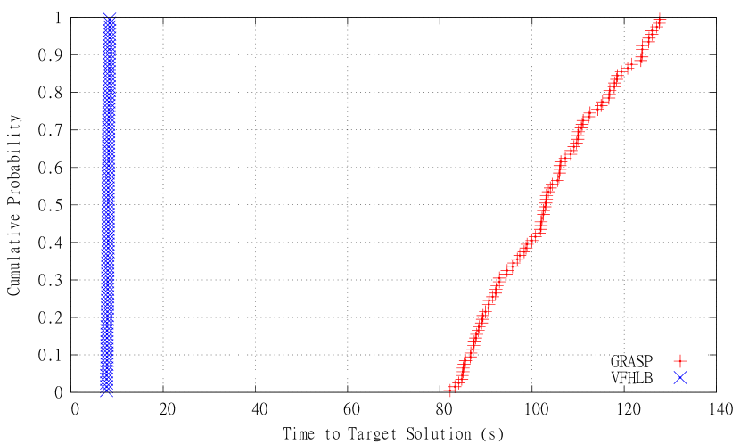
(a) TTTPlot: 20-0.8-30-1

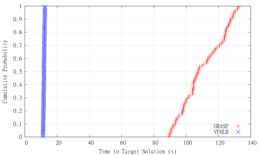
(b) TTTPlot: 20-0.8-30-2

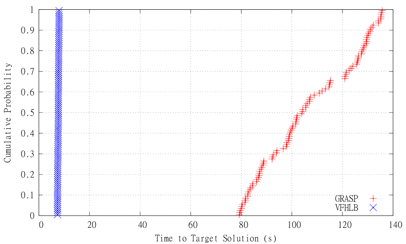
(c) TTTPlot: 20-0.8-30-3

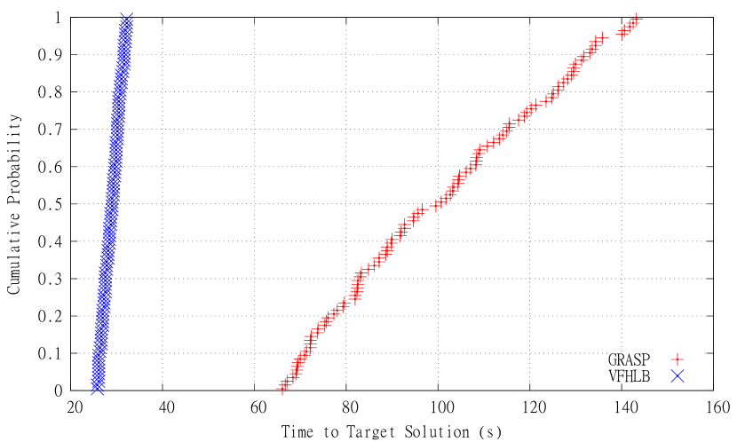
(d) TTTPlot: 20-0.8-30-4

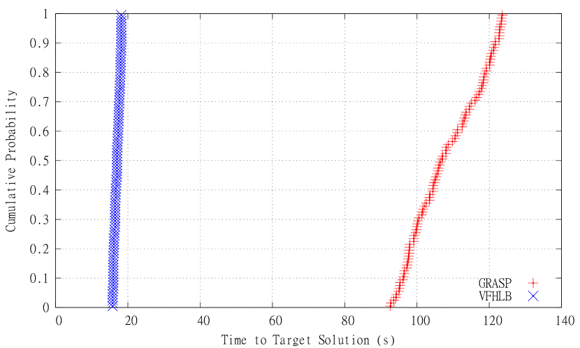
(e) TTTPlot: 20-0.8-30-5

Figure 1: TTT Plot - 20 Nodes Instances

After analyzing the behavior of the methods for the selected instances of 20 nodes, through analysis of the TTTPlot figures 1(a) to 1(e), we conclude that the proposed strategy outperforms the GRASP, since the cumulative probability for VFHLB to find the target in less then 40 seconds is 100 $\%$, while for GRASP it is 0 $\%$.

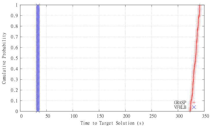
(a) TTTPlot: 30-0.8-30-1

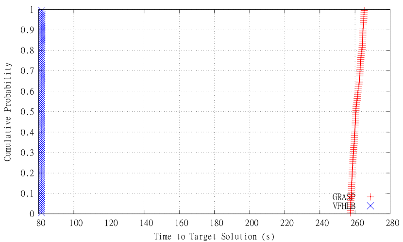
(b) TTTPlot: 30-0.8-30-2

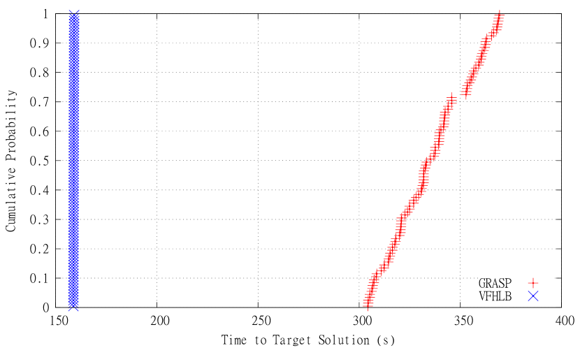
(c) TTTPlot: 30-0.8-30-3

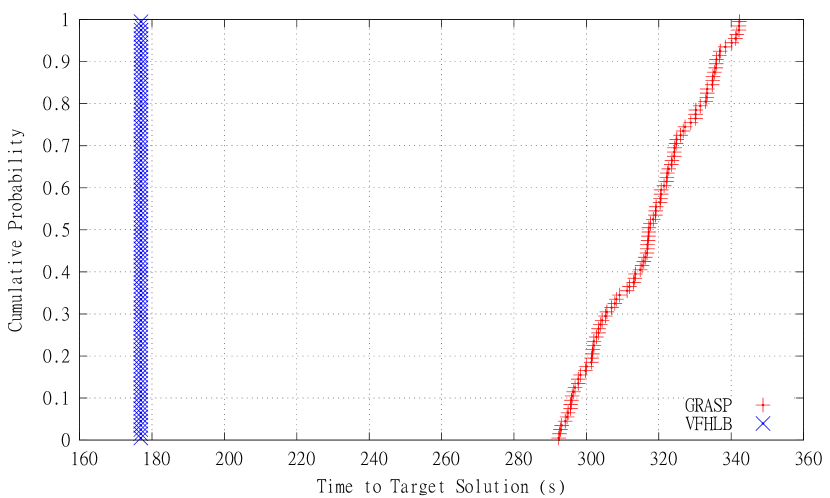
(d) TTTPlot: 20-0.8-30-4

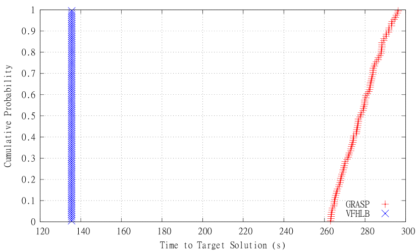
(e) TTTPlot: 30-0.8-30-5

Figure 2: TTT Plot - 30 Nodes Instances

After analyzing the behavior of the methods for the selected instances of 30 nodes, through analysis of the TTTPlot figures 2(a) to 2(e), we conclude that the proposed strategy outperforms the GRASP, since the cumulative probability for VFHLB to find the target in less then 180 seconds is 100 $\%$, while for GRASP it is 0 $\%$.

CONCLUSIONS

We proposed a new algorithm for a variant of the fixed-charge uncapacitated network design problem where multiple shortest path problems were taken into consideration. In the first phase of the algorithm, the VFH is used to build a initial solution and find a lower bound. In a second moment, a Local Branching technique and a pertubation, Ejection Cycle, are applied to reduce the solution cost.
The proposed approach was tested on a set of instances grouped by number of nodes, graph density and number of commodities to be transported. Our results have shown the efficiency of VFHLB in comparison with the GRASP presented in [14], since the proposed algorithm finds the optimal solution for all instances and presents a best average time for the majority of the instances (125 out 135).
As future work, we intend to work on exact approaches as Benders’ Decomposition and Lagrangian Relaxation since both are very effective for similar problems, as could be seen in [5, 10].

References

- Ahuja et al. [1993] Ahuja, R. K., Magnanti, T. L., Orlin, J. B., 1993. Network flows: theory, algorithms, and applications. Prentice-Hall, Inc., Upper Saddle River, NJ, USA.
- Aiex, R. M. and Resende, M. G. C. and Ribeiro, C. C. [2007] Aiex, R. M. and Resende, M. G. C. and Ribeiro, C. C., 2007. Ttt plots: a perl program to create time-to-target plots. Optimization Letters 1 (4), 355–366.
- Amaldi et al. [2011] Amaldi, E., Bruglieri, M., Fortz, B., 2011. On the hazmat transport network design problem. In: Proceedings of the 5th international conference on Network optimization. INOC’11. Springer-Verlag, Berlin, Heidelberg, pp. 327–338.
- Bazaraa et al. [2004] Bazaraa, M. S., Jarvis, J. J., Sherali, H. D., 2004. Linear Programming and Network Flows. Wiley-Interscience.
-
Bektas et al. [2007]
Bektas, T., Crainic, T. G., Gendron, B., May 2007. Lagrangean decomposition for
the multicommodity capacitated network design problem. In: Optimization Days
2007.
URL http://eprints.soton.ac.uk/55826/ - Billheimer and Gray [1973] Billheimer, J. W., Gray, P., feb 1973. Network Design with Fixed and Variable Cost Elements. Transportation Science 7 (1), 49–74.
- Boesch [1976] Boesch, F. T., 1976. Large-scale Networks: Theory and Design, 1st Edition. IEEE Press selected reprint series.
- Boyce and Janson [1980] Boyce, D., Janson, B., mar 1980. A discrete transportation network design problem with combined trip distribution and assignment. Transportation Research Part B: Methodological 14 (1-2), 147–154.
- Colson et al. [2005] Colson, B., Marcotte, P., Savard, G., jun 2005. Bilevel programming: A survey. 4OR 3 (2), 87–107.
- Costa et al. [2009] Costa, A. M., Cordeau, J.-F., Gendron, B., 2009. Benders, metric and cutset inequalities for multicommodity capacitated network design. Computational Optimization and Applications 42 (3), 371–392.
- Erkut and Gzara [2008] Erkut, E., Gzara, F., jul 2008. Solving the hazmat transport network design problem. Computers & Operations Research 35 (7), 2234–2247.
- Erkut et al. [2007] Erkut, E., Tjandra, S. A., Verter, V., 2007. Hazardous Materials Transportation. In: Handbooks in Operations Research and Management Science. Vol. 14. Ch. 9, pp. 539–621.
- Fischetti and Lodi [2003] Fischetti, M., Lodi, A., sep 2003. Local branching. Mathematical Programming 98 (1-3), 23–47.
- González et al. [2013] González, P. H., Martinhon, C., Simonetti, L., Santos, E., Michelon, P., 2013. Uma Metaheurística GRASP para o Problema de Planejamento de Redes com Rotas Ótimas para o Usuário. In: XLV Simpósio Brasileiro de Pesquisa Operacional. Natal, pp. 1813–1824.
- Graves and Lamar [1983] Graves, S. C., Lamar, B. W., may 1983. An Integer Programming Procedure for Assembly System Design Problems. Operations Research 31 (3), 522–545.
- Hettmansperger and McKean [1998] Hettmansperger, T. P., McKean, J. W., 1998. Robust nonparametric statistical methods. CRC Press.
- Holmberg and Yuan [2004] Holmberg, K., Yuan, D., jan 2004. Optimization of Internet Protocol network design and routing. Networks 43 (1), 39–53.
- Johnson et al. [1978] Johnson, D. S., Lenstra, J. K., Kan, A. H. G. R., jan 1978. The complexity of the network design problem. Networks 8 (4), 279–285.
- Kara and Verter [2004] Kara, B. Y., Verter, V., may 2004. Designing a Road Network for Hazardous Materials Transportation. Transportation Science 38 (2), 188–196.
- Kimemia and Gershwin [1978] Kimemia, J., Gershwin, S., 1978. Network flow optimization in flexible manufacturing systems. In: 1978 IEEE Conference on Decision and Control including the 17th Symposium on Adaptive Processes. IEEE, pp. 633–639.
- Lourenço and S. [2010] Lourenço, H., O. M., S., T., 2010. Handbook of Metaheuristics. Vol. 146 of International Series in Operations Research & Management Science. Springer US, Boston, MA.
- Luigi De Giovanni [2004] Luigi De Giovanni, 2004. The Internet Protocol Network Design Problem with Reliability and Routing Constraints. Ph.D. thesis, Politecnico di Torino.
- Magnanti [1981] Magnanti, T. L., jan 1981. Combinatorial optimization and vehicle fleet planning: Perspectives and prospects. Networks 11 (2), 179–213.
- Magnanti and Wong [1984] Magnanti, T. L., Wong, R. T., feb 1984. Network Design and Transportation Planning: Models and Algorithms. Transportation Science 18 (1), 1–55.
- Mandl [1981] Mandl, C. E., aug 1981. A survey of mathematical optimization models and algorithms for designing and extending irrigation and wastewater networks. Water Resources Research 17 (4), 769–775.
- Mauttone et al. [2008] Mauttone, A., Labbé, M., Figueiredo, R. M. V., 2008. A Tabu Search approach to solve a network design problem with user-optimal flows. In: V ALIO/EURO Conference on Combinatorial Optimization. Buenos Aires, pp. 1–6.
- Paraskevopoulos et al. [2013] Paraskevopoulos, D. C., Bektaş, T., Crainic, T. G., Potts, C. N., 2013. A Cycle-Based Evolutionary Algorithm for the Fixed-Charge Capacitated Multi-Commodity Network Design Problem. Tech. rep., Centre interuniversitaire de recherche sur les réseaux d’entreprise, la logistique et le transport, Montreal.
- Simpson [1969] Simpson, R. W., 1969. Scheduling and routing models for airline systems. Massachusetts Institute of Technology, Flight Transportation Laboratory.
- Wolsey [1998] Wolsey, L. A., 1998. Integer programming. Wiley-Interscience, New York, NY, USA.
- Wong [1978] Wong, R. T., 1978. Accelerating Benders decomposition for network design. Ph.D. thesis, Massachusetts Institute of Technology.
- Wong [1980] Wong, R. T., mar 1980. Worst-Case Analysis of Network Design Problem Heuristics. SIAM Journal on Algebraic Discrete Methods 1 (1), 51–63.