Probing quantum-classical boundary with compression software

Abstract

We experimentally demonstrate that it is impossible to simulate quantum bipartite correlations with a deterministic universal Turing machine. Our approach is based on the Normalized Information Distance (NID) that allows the comparison of two pieces of data without detailed knowledge about their origin. Using NID, we derive an inequality for output of two local deterministic universal Turing machines with correlated inputs. This inequality is violated by correlations generated by a maximally entangled polarization state of two photons. The violation is shown using a freely available lossless compression program. The presented technique may allow to complement the common statistical interpretation of quantum physics by an algorithmic one.

I Introduction

The idea that physical processes can be considered as computations done on some universal machines traces back to Turing and von Neumann Coveney and Highfield (1996), and the growth of the computational power allowed for further development of these concepts. This resulted in a completely new approach to science in which the complexity of observed phenomena is closely related to the complexity of computational resources needed to simulate them Wolfram (1985). In addition, there are physical phenomena that simply cannot be traced with analytical tools, which further motivated a computational approach to physics Moore (1990). Moreover, the idea of quantum computation Feynman (1982) lead to a discovery of a few problems that seem not efficiently traceable on classical computers but efficiently on a quantum version Shor (1994); Grover (1996).

Classical physics can be simulated on universal Turing machines, or other computationally equivalent models Wolfram (2001). On the other hand, efficient simulation of quantum systems requires a replacement of deterministic universal Turing machines with quantum computers whose states are non-classically correlated. Such machines can even simulate any local quantum system efficiently Deutsch (1985); Lloyd (1996). Can we experimentally distinguish between these two descriptions of the universe using a logically self-contained computational approach?

In this paper, we show that there are processes which cannot be simulated on local classical machines at all, independently of the available classical resources. We first introduce the notion of Kolmogorov complexity, a measure of the classical complexity of a phenomena, and later apply it to derive a bound on classical descriptions Li et al. (2004). Next, we use the fact that Kolmogorov complexity can be approximated by compression algorithms Cilibrasi and Vitányi (2005).

We compress experimental data obtained from polarisation measurements on entangled photon pairs and show the violation of a classical bound.

Let’s consider the description of a machine, whether classical or quantum, that outputs a string $x$ made of 0’s and 1’s. In the case of a Turing machine $U$, we can always write a program $\Lambda$ that generates $x$. The simplest such program is obviously ‘PRINT $x$’. However, this is not optimal: in many cases the program can be much shorter than the string itself.

This brings us to the concept of Kolmogorov complexity $K(x)$, the minimal length $l(\Lambda)$ of all programs $\Lambda$ that reproduce a specific output $x$. If $K(x)$ is of the order of the length of the output $l(x)$ then our algorithmic description of $x$ is inefficient, and $x$ is called algorithmically random Li and Vitanyi (2009). In most cases $K(x)$ cannot be computed Cover and Thomas (2006). To circumvent this issue, we can estimate $K(x)$ with some efficient lossless compression algorithm $C(x)$ Cilibrasi and Vitányi (2005).

We now extend this picture by considering two Turing machines $U_{A}$ (Alice) and $U_{B}$ (Bob), which are spatially separated. If these machines cannot communicate, they generate two output strings that are independent, although the programs fed into the machines can be correlated. Moreover, the input programs are classical bit strings so the correlations between them must be classical.

We determine the complexity of the generated strings using the Normalized Information Distance (NID) Li et al. (2004). This distance allows for a comparison of two data sets without detailed knowledge about their origin. In practice, we evaluate an approximation to the NID, the Normalized Compression Distance (NCD) Cilibrasi and Vitányi (2005), using a lossless compression software, in our case the LZMA Utilities, based on the Lempel-Ziv-Markov chain algorithm Pavlov .

II Simulation by deterministic universal Turing machines

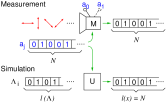
Figure 1: Measurement: $N$ particles enter a measuring device, characterized by two possible polarizer settings $a_{0}$ and $a_{1}$, which generates a bit string of $N$ measurement outcomes. Simulation: a universal Turing machine is fed with a program elements $\Lambda_{i}$ and information about the chosen setting $a_{0}$ or $a_{1}$. It delivers an output string of length $N$.

We consider a model experiment, similar to the one used for testing the Bell inequalities Bell (1964): a source emits pairs of photons that travel to two separate polarization analyzers M_A (Alice) and M_B (Bob). Each analyzer has two outputs associated with bit values 0 and 1, and can be set along directions $a_{0}$ or $a_{1}$ for M_A, and $b_{0}$ or $b_{1}$ for M_B. The record of the outputs from each analyzer forms a bit string (see Fig. 1).

The output $x$ of each individual analyzer can be described as the output of a Turing machine $U$, fed with the settings $a_{j}$ or $b_{k}$, and a program $\Lambda$. The program will contain the information for generating the correct output for every detection event and for every setting.

If we consider a string of finite length $l(x)=N$, $\Lambda$ will have to describe the $4^{N}$ possible events. The length of the shortest $\Lambda$ is equal to the Kolmogorov complexity of the generated string.

Next, we consider the simulation of the experiment with two local non-communicating machines $U_{A}$ and $U_{B}$ (see Fig. 2). We feed a program $\Lambda$ to both of them and obtain two output strings, $x$ and $y$, both of length $N$. In this case, the program has to describe the behavior of all $2N$ events for all possible settings $a_{j}$ and $b_{k}$, hence $16^{N}$ possible events.

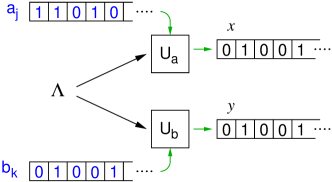
Figure 2: Local classical machines simulating the generation of strings $x$ and $y$ by correlation measurements on an entangled state.

II.1 Normalized Information Distance

The Kolmogorov complexity of two bit strings $K(x,y)$ is the length of the shortest program generating them simultaneously. $K(x,y)$ can be shorter than $K(x)\,+\,K(y)$ if $x$ and $y$ are correlated - the more correlated they are, the simpler it is to compute one string knowing the other. This idea was further carried out by Cilibrasi and Vitanyi Cilibrasi and Vitányi (2005) who constructed a distance measure between $x$ and $y$ called Normalized Information Distance (NID),

$$\text{NID}(x,y)\,=\,\frac{K(x,y)\,-\,\min\{K(x),K(y)\}}{\max\{K(x),K(y)\}}\,.$$ (1)

The NID obeys all required properties of a metric, in particular, the triangle inequality

$$\text{NID}(x,y)\,+\,\text{NID}(y,z)\,\geq\,\text{NID}(x,z)\,.$$ (2)

The above inequality holds up to a correction of order $\log(l(x))$, which can be neglected for sufficiently long strings Cilibrasi and Vitányi (2005).

II.2 Information Inequality

We consider the bit strings $x_{a_{j}}$ and $y_{b_{k}}$ generated by Alice and Bob with fixed setting $a_{j}$ and $b_{k}$. Equation (2) then transforms into

$$\text{NID}(x_{a_{0}},y_{b_{0}})+\text{NID}(y_{b_{0}},y_{b_{1}})\geq\text{NID}(x_{a_{0}},y_{b_{1}})\,.$$ (3)

However, $\text{NID}(y_{b_{0}},y_{b_{1}})$ cannot be determined experimentally because the strings $y_{b_{0}}$ and $y_{b_{1}}$ come from measurements of incompatible observables. We therefore use the triangle inequality

$$\text{NID}(x_{a_{1}},y_{b_{0}})+\text{NID}(x_{a_{1}},y_{b_{1}})\geq\text{NID}(y_{b_{0}},y_{b_{1}})\,,$$ (4)

and combine it with inequality (3) to obtain a quadrangle inequality:

$$\text{NID}(x_{a_{0}},y_{b_{0}})+\text{NID}(x_{a_{1}},y_{b_{0}})+ \text{NID}(x_{a_{1}},y_{b_{1}})\geq$$ (5)

$$\text{NID}(x_{a_{0}},y_{b_{1}}).$$

Similar to various tests of Bell inequalities, we introduce a scalar quantity $S^{\prime}$ that quantifies the degree of violation of Eq. (5):

$$S^{\prime} = \text{NID}(x_{a_{0}},y_{b_{1}})-\text{NID}(x_{a_{0}},y_{b_{0}})$$ (6)

$$- \text{NID}(x_{a_{1}},y_{b_{0}})\,-\,\text{NID}(x_{a_{1}},y_{b_{1}})\leq 0$$

In order to experimentally test this inequality, we have to address the following problem. We can set up a source to generate entangled photon pairs in a state of our choosing, but we cannot control the nature of the measurement. For every experimental run $i$ with the same preparation the resulting string $x_{i,a_{j}}$ can be different. Consequently, the corresponding program $\Lambda_{i}$ is different for every experimental run.

It is reasonable to assume that for every two experimental runs $i$ and $i^{\prime}$ the complexity of the generated strings remains the same: $K(x_{i,a_{j}})\,=\,K(x_{i^{\prime},a_{j}})$ and $K(x_{i,a_{j}},y_{i,b_{k}})\,=\,K(x_{i^{\prime},a_{j}},y_{i^{\prime},b_{k}})$. Without these assumptions the same physical preparation of the experiment has different consequences and thus the notion of preparation loses its meaning. More generally, the predictive power of science can be expressed by saying that the same preparation results in the same complexity of observed phenomena.

III Estimation of Kolmogorov complexity

In general the Kolmogorov complexity cannot be evaluated, but it can be estimated. One can adapt two conceptually different approaches.

III.1 Statistical Approach

This approach takes into account the ensemble of all possible $N$-bit strings and asks about their average Kolmogorov complexity. It can be shown that this average equals the Shannon entropy $H(X)$ of the ensemble Cover and Thomas (2006), and thus

$$\langle\text{NID}(x,y)\rangle=\frac{H(x,y)-\min\{H(x),H(y)\}}{\max\{H(x),H(y)\}}\,.$$ (7)

Inequality (5) becomes a type of entropic Bell inequality introduced by Braunstein and Caves Braunstein and Caves (1988) if local entropies are maximal, i.e., $H(x)=H(y)=N$. They showed that for a maximally entangled polarization state of two photons, and polarizer angles obeying the constraints

$$\vec{a_{0}}\cdot\vec{b_{1}} = \cos 3\theta\,,$$

$$\vec{a_{0}}\cdot\vec{b_{0}} = \vec{a_{1}}\cdot\vec{b_{0}}=\vec{a_{1}}\cdot\vec{b_{1}}=\cos\theta\,,$$ (8)

inequality (5) is violated for an appropriate range of $\theta$. Calculating the entropy $H(x,y)$ using the probability distributions predicted by quantum mechanics, it is possible to obtain the expected value of $S^{\prime}$ as a function of $\theta$ (Fig. 4a). The maximal violation of this inequality is $S^{\prime}=0.24$, with a separation of $\theta\,=\,8.6^{\circ}$.

III.2 Algorithmic approach

It is possible to avoid a statistical description of our experiment following the ideas pioneered in Cilibrasi and Vitányi (2005). There, it was shown that the Kolmogorov complexity can be well approximated by the application of compression algorithms. This approximation introduces the new distance called Normalized Compression Distance (NCD)

$$\text{NCD}(x,y)=\frac{C(x,y)-\min\{C(x),C(y)\}}{\max\{C(x),C(y)\}}\,,$$ (9)

where $C(x)$ is the length of the compressed string $x$, and $C(x,y)$ is the length of the compressed concatenated strings $x,y$. Replacing NID with NCD in Eq. (6) leads to a new inequality:

$$S^{\prime}\rightarrow S = \text{NCD}(x_{a_{0}},y_{b_{1}})-\text{NCD}(x_{a_{0}},y_{b_{0}})$$ (10)

$$- \text{NCD}(x_{a_{1}},y_{b_{0}})-\text{NCD}(x_{a_{1}},y_{b_{0}})\leq 0\,.$$

This expression can be tested experimentally because the NCD distance measure is operationally defined.

IV Choice of compressor

Before moving to the experiment, we need to ensure the suitability of the compression software we use to evaluate the NCD. For this, we numerically simulate the outcome of an experiment, based on a distribution of results predicted by quantum physics. Among the packages we tested, we found that the LZMA Utility Pavlov approaches the Shannon limit Shannon (1948) most closely.

The simulation also allows us to verify the angle that maximizes the violation of Eq. (10) predicted from Eq. (8). The results of the simulation are presented in Fig. 4. More details on the generation of the simulated data and the choice of the compressor are provided in the Appendix.

V Experiment

In our experiment (see Fig. 3), the output of a grating-stabilized laser diode (LD, central wavelength 405 nm) passes through a single mode optical fiber (SMF) for spatial mode filtering, and is focused to a beam waist of 80 ${\mu}$m into a 2 mm thick BBO crystal. In this crystal (cut for type-II phase-matching), photon pairs are generated via spontaneous parametric down-conversion (SPDC) in a slightly non-collinear configuration. A half-wave plate ($\lambda$/2) and a pair of compensation crystals (CC) take care of the temporal and transversal walk-off Kwiat et al. (1995).

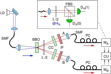
Figure 3: Schematic of the experimental set-up. Polarization correlations of entangled-photon pairs are measured by the polarization analyzers M_A and M_B, each consisting of a half wave plate ($\lambda/2$) followed by a polarization beam splitter (PBS). All photons are detected by Avalanche photodetectors D_H and D_V, and registered in a coincidence unit (CU).

Two spatial modes (labeled A and B) of down-converted light, defined by the SMFs for 810 nm, are matched to the pump mode to optimize the collection Kurtsiefer et al. (2001). In type-II SPDC, each down-converted pair consists of an ordinary and extraordinarily polarized photon, corresponding to horizontal (H) and vertical (V) in our setup. A pair of polarization controllers (PC) ensures that the SMFs do not affect the polarization of the collected photons. To arrive at an approximate singlet Bell state, the phase $45^{\circ}$ between the two decay possibilities in the polarization state

$$|{\psi}\rangle={1\over\sqrt{2}}\left(|{H}\rangle_{A}|{V}\rangle_{B}+e^{i45^{\circ}}|{V}\rangle|{H}\rangle_{B}\right),$$ (11)

is adjusted to $45^{\circ}$ = $\pi$ by tilting the CC.

In the polarization analyzers (Fig. 3), the photons from SPDC are projected onto arbitrary linear polarization by $\lambda$/2 plates, set to half of the analyzing angles $\theta_{A(B)}$, and polarization beam splitter (PBS) in each analyzer. Photons are detected by avalanche photo diodes (APDs), and corresponding detection events from the same pair identified by a coincidence unit (CU) if they arrive within $\approx\pm$3 ns of each other.

The quality of polarization entanglement is tested by probing the polarization correlations in a basis complementary to the intrinsic HV basis of the crystal; for Bell states $|{\psi^{\pm}}\rangle$, strong polarization correlations are e.g. expected in a $\pm$ 45^∘ linear polarization basis.

With interference filters (IF) of 5 nm bandwidth (FWHM) centered at 810 nm, we observe a visibility $V_{45}$ = 99.9$\pm$0.1%. The visibility in the natural H/V basis of the type-II down-conversion process also reaches $V_{\rm HV}$ = 99.9$\pm$0.1%. A separate test of a CHSH-type Bell inequality Clauser et al. (1969) leads to a value of $S=2.826\pm 0.0015$. This indicates a relatively high quality of polarization entanglement; the uncertainties in the visibilities are obtained from propagated Poissonian counting statistics.

V.1 Measurement and Data Post-processing

We record two-fold coincidences of detection events between detectors at A and B. For each PBS, the transmitted output is associated with 0 and the reflected one with 1. The resulting binary strings $x$ from A, and $y$ from B are written into two individual binary files. From these, we calculate the NCD using Eq. (9). This procedure is repeated for each of the four settings ($a_{0},b_{0}$), ($a_{1},b_{0}$), ($a_{1},b_{1}$), and ($a_{0},b_{1}$) in order to obtain the value for $S$.

To remove the bias due to differences in the detection efficiency of the APDs in the experiment, we also measure for each setting the associated orthogonal ones (see Appendix for details).

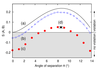
Figure 4: Plots of $S$ versus angle of separation $\theta$. (a) Result obtained from Eq. (7) (b) result obtained from using the LZMA compressor on a simulated data ensemble, (c) measurement of $S$ in the experiment shown in Fig. 3, and (d) longer measurement at the optimal angle $\theta=8.6^{\circ}$.

VI Results

The inequality is experimentally tested by evaluating $S$ in Eq. (10) for a range of $\theta$; the obtained values [points (c), (d) in Fig. 4] are consistently lower than the trace (a) calculated via entropy using Eq. (7), and than a simulation with the same compressor (b). This is because the LZMA Utility is not working exactly at the Shannon limit, and also due to imperfect state generation and detection.

As a consequence of Eq. (8), we expect the maximal violation for $\theta=8.6^{\circ}$. For this particular angle we collected results from a large number of photon pairs. Although we set out in this work to avoid a statistical argument in the interpretation of measurement results, we do resort to statistical techniques to assess the confidence in an experimental finding of a violation of inequality Eq. (10). To estimate an uncertainty of the experimentally obtained values for $S$, this large data set was subdivided into files with length greater than $10^{5}$ bits. The results from all the subdivided files are then averaged to obtain the final result of $S(\theta=8.6^{\circ})$= 0.0494$\,\pm\,$0.0076, with the latter indicating a relatively small standard deviation over these different subsets.

VII Conclusion

There is a trend to look at physical systems and processes as programs run on a computer made of the constituents of our universe. We could show that this is not possible if one uses a computation paradigm of a local deterministic Turing machine. Although this has been already extensively researched in quantum information theory, we present a complementary algorithmic approach for an explicit, experimentally testable example. This algorithmic approach is complementary to the orthodox Bell inequality approach to quantum nonlocality Bell (1964) that is statistical in its nature.

Any process that can be simulated on a local universal Turing machine can be encoded as a program that is fed into it. For every such a program there exists its shortest description called Kolmogorov complexity, which in most of the cases can only be approximated using compression software. Moreover, such a description must obey distance properties as shown in Li et al. (2004); Cilibrasi and Vitányi (2005). By testing Eq. (10), we showed that this is unattainable in the specific case of polarization-entangled photon pairs. Therefore, there exist physical processes that cannot be simulated on local universal Turing machines.

There are two fundamentally different notions of complexity in computer science. On one hand, computational complexity, mainly researched on in quantum information science, studies how much resources are needed to solve a computational problem. These studies focus on complexity classes such as P, NP Papadimitriou (1994), and its main concern is, given an input program, how efficiently it can be computed. On the other hand, algorithmic complexity deals with a problem of what the most efficient encoding of an input program is. This complementary problem to computation complexity has not yet received enough attention in quantum information science, and it would require a further work on quantum version of Kolmogorov complexity Mueller (2007).

We would like to stress that our analysis of the experimental data is purely and consistently algorithmic. We do not resort to statistical methods that are alien to the concept of computation. If this approach can be extended to all quantum experiments, it would allow us to bypass the commonly used statistical interpretation of quantum theory.

VIII Acknowledgments

We acknowledge the support of this work by the National Research Foundation & Ministry of Education in Singapore, partly through the Academic Research Fund MOE2012-T3-1-009. P.K. and D.K. are also supported by the Foundational Questions Institute (FQXi). A.C. also thanks Andrea Baronchelli for the hints on the use of compression software.

IX Appendix: Symmetrization of detector efficiencies

The experimental setup (Fig. 3) uses four APDs: $D_{HA}$, $D_{VA}$ (Alice), and $D_{HB}$, $D_{VB}$ (Bob) to register photon pair events in the two spatial modes. By denoting events at $D_{H}$ and $D_{V}$ as 1 and 0, the four possible output patterns are 00, 01, 10, and 11, where the least and most significant bit corresponds to the Alice and Bob mode, respectively. Due to differences in the the losses in the transmitted and reflected port of the PBS, efficiencies in coupling light into the APDs, and the quantum efficiencies of APDs, the detection efficiencies for the four output combinations are different. The resulting effective pair efficiencies are then given by the product of the contributing detection efficiencies $\eta_{VB}$, $\eta_{HB}$, $\eta_{VA}$, and $\eta_{HA}$.

This asymmetry will skew the statistics of the measurement results. We symmetrize the effective pair efficiencies for each $(\theta_{A},\theta_{B})$ measuring also the following settings: $(\theta_{A}+45^{\circ},\theta_{B})$, $(\theta_{A},\theta_{B}+45^{\circ})$, and $(\theta_{A}+45^{\circ},\theta_{B}+45^{\circ})$. This procedure swaps the output ports of the PBS at which each polarization state is detected. The resulting outcomes are then interleaved, providing an uniform detection probability for the four possible outcomes. The effective pair detection efficiency for all four combinations is then $(\eta_{VB}\,\eta_{VA}\,+\,\eta_{VB}\,\eta_{HA}\,+\,\eta_{HB}\,\eta_{VA}\,+\,\eta_{HB}\,\eta_{HA})/4$.

X Appendix: Choice of compressor

In order to evaluate the NCDs of the binary strings, we need to choose a compression algorithm that performs close to the Shannon limit. This is necessary to ensure that it does not introduce any unintended artifacts that lead to an overestimation of the violation. Preferably we want to work in the regime where the obtained NCDs always underestimate the violation. For this purpose, we characterized four compression algorithms implemented by freely available compression programs: lzma Pavlov , bzip2 Seward , gzip Gailly and Adler , and lzw Welch (1984). To eliminate the overhead associated with the compression of ASCII text files, we save data in a binary format.

For this characterization and a simulation of the experiment, we need to generate a “random” string of bits (1, 0) or pairs of bits (00, 01, 10, and 11) of various length with various probability distributions. We generate these strings using the MATLAB ref function randsample() that uses the pseudo random number generator mt19937ar with a long period of $2^{19937}-1$. It is based on the Mersenne Twister Matsumoto and Nishimura (1998), with ziggurat Marsaglia and Tsang (2000) as the algorithm that generates the required probability distribution. The complexity of this (deterministic) source of pseudorandom numbers should be high enough to not be captured as algorithmic.

The first part of this characterization involves establishing the minimum string length required for the compression algorithms to perform consistently. We start by generating binary strings, $x$, with equal probability of 1’s and 0’s, i.e. random strings, of varying length. For each $x$, we evaluate the compression overhead $Q$ as

$$Q=\frac{C(x)-H(x)}{l(x)}\,.$$ (12)

For a good compressor, we expect $Q$ to be close to 0. From Fig. 5, it can be seen that for all the compressors, $Q$ starts to converge after about $10^{5}$ bits, setting the minimum string length required for the compressors to work consistently. The lzw compressor fails this test, converging to a $Q$ of 0.37 for long string, while bzip2, gzip, and lzma give a $Q$ below $10^{-1}$.

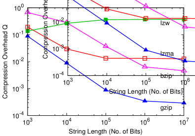
Figure 5: Comparison of the compression overhead $Q$ obtained using four different compression algorithms on pseudo-random strings of varying lengths. The expected value for an ideal compressor is 0. From this characterization we can exclude lzw as a useful compressor for our application.

In the second part of this characterization, test the compressors with strings with a known amount of correlation. We generate a random string $x$ of length $10^{7}$ using the same technique already described. We then generate a second string $y$ of equal length and with probability $p$ of being correlated to $x$. For $p=0$ the two strings are equal, i.e. perfectly correlated. For $p=0.5$ they are uncorrelated.

The two strings $x$ and $y$ are then combined to form the string $xy$: to avoid artifacts due to the limited data block size of the compression algorithms, the elements of $x$ and $y$ are interleaved. We then compress $xy$ and evaluate the compression overhead $Q$ as a function of $p$. The results for different compressors are shown in Fig. 6. Although there are ranges of $p$ where bzip and gzip perform better than lzma, the latter shows a more uniform performance over the entire interval of $p$. It is reasonable to assume that the use of lzma should reduce the possibility of artifacts in the estimation of the NCD also for the data obtained from the experiment.

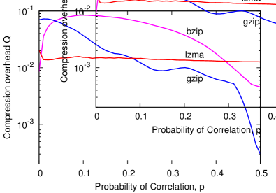
Figure 6: Compression overhead $Q$ for the string $xy$ as a function of the probability of pairwise correlation $p$ between the bits of the generating strings $x$ and $y$ for three different compressors: bzip, gzip, and lzma.

References

- Coveney and Highfield (1996) P. V. Coveney and R. Highfield, Frontiers of Complexity: The Search for Order in a Chaotic World (Fawcett Columbine, 1996).
- Wolfram (1985) S. Wolfram, Phys. Rev. Lett. 54, 735 (1985).
- Moore (1990) C. Moore, Phys. Rev. Lett. 64, 2354 (1990).
- Feynman (1982) R. P. Feynman, Int. J. Theor. Phys. 21, 467 (1982).
- Shor (1994) P. W. Shor, in Proceedings of the 35th Annual Symposium on Foundations of Computer Science (IEEE, Santa Fe, NM, 1994) pp. 124–134.
- Grover (1996) L. K. Grover, in Proceedings, 28th Annual ACM Symposium on the Theory of Computing (1996) p. 212.
- Wolfram (2001) S. Wolfram, New Kind of Science? (Wolfram Media, Inc., 2001).
- Deutsch (1985) D. Deutsch, Proceedings of the Royal Society of London A: Mathematical, Physical and Engineering Sciences 400, 97 (1985).
- Lloyd (1996) S. Lloyd, Science 273, 1073 (1996).
- Li et al. (2004) M. Li, X. Chen, X. Li, B. Ma, and P. M. B. Vitányi, Information Theory, IEEE Transactions on 50, 3250 (2004).
- Cilibrasi and Vitányi (2005) R. Cilibrasi and P. M. B. Vitányi, Information Theory, IEEE Transactions on 51, 1523 (2005).
- Li and Vitanyi (2009) M. Li and P. M. B. Vitanyi, An Introduction to Kolmogorov Complexity and Its Applications, Texts in Computer Science (Springer New York, 2009).
- Cover and Thomas (2006) T. M. Cover and J. A. Thomas, Elements of Information Theory, 2nd ed. (Wiley-Interscience, 2006).
- (14) I. Pavlov, http://www.7-zip.org/sdk.html.
- Bell (1964) J. S. Bell, Physics 1, 195 (1964).
- Braunstein and Caves (1988) S. L. Braunstein and C. M. Caves, Phys. Rev. Lett. 61, 662 (1988).
- Shannon (1948) C. E. Shannon, Bell System Technical Journal 27, 379 (1948).
- Kwiat et al. (1995) P. G. Kwiat, K. Mattle, H. Weinfurter, A. Zeilinger, A. V. Sergienko, and Y. Shih, Phys. Rev. Lett. 75, 4337 (1995).
- Kurtsiefer et al. (2001) C. Kurtsiefer, M. Oberparleiter, and H. Weinfurter, Phys. Rev. A 64, 023802 (2001).
- Clauser et al. (1969) J. F. Clauser, M. Horne, A. Shimony, and R. Holt, Phys. Rev. Lett. 23, 880 (1969).
- Papadimitriou (1994) C. H. Papadimitriou, Computational Complexity, Theoretical computer science (Addison-Wesley, 1994).
- Mueller (2007) M. Mueller, Quantum Kolmogorov Complexity and the Quantum Turing Machine, Ph.D. thesis, Technical University of Berlin, Berlin (2007).
- (23) J. Seward, http://www.bzip.org/.
- (24) J.-l. Gailly and M. Adler, http://www.gzip.org/.
- Welch (1984) T. Welch, Computer 17, 8 (1984).
- (26) MATLAB R2010a, The MathWorks, Inc., Natick, Massachusetts, United States.
- Matsumoto and Nishimura (1998) M. Matsumoto and T. Nishimura, ACM Transactions on Modeling and Computer Simulation (TOMACS) 8, 3 (1998).
- Marsaglia and Tsang (2000) G. Marsaglia and W. W. Tsang, Journal of Statistical Software 5, 1 (2000).