Connected components of meanders:
I. Bi-rainbow meanders
Anna Karnauhova
anna.karnauhova@math.fu-berlin.de
Stefan Liebscher
stefan.liebscher@fu-berlin.de
Freie Universität Berlin, Institut für Mathematik
Arnimallee 3, 14195 Berlin, Germany
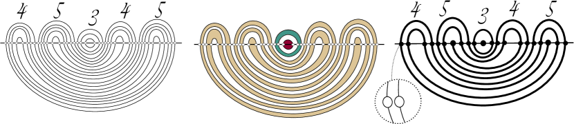
![[Uncaptioned image]](/html/1504.03099/assets/FigCoverArt.jpg)
draft version of April 13, 2015
Abstract
Closed meanders are planar configurations of one or several disjoint closed Jordan curves intersecting a given line or curve transversely. They arise as shooting curves of parabolic PDEs in one space dimension, as trajectories of Cartesian billiards, and as representations of elements of Temperley-Lieb algebras.
Given the configuration of intersections, for example as a permutation or an arc collection, the number of Jordan curves is unknown and needs to be determined.
We address this question in the special case of bi-rainbow meanders, which are given as non-branched families (rainbows) of nested arcs. Easily obtainable results for small bi-rainbow meanders containing up to four families suggest an expression of the number of curves by the greatest common divisor (gcd) of polynomials in the sizes of the rainbow families.
We prove however, that this is not the case. In fact, the number of connected components of bi-rainbow meanders with more than four families cannot be expressed as the gcd of polynomials in the sizes of the rainbows.
On the other hand, we provide a complexity analysis of nose-retraction algorithms. They determine the number of connected components of arbitrary bi-rainbow meanders in logarithmic time. In fact, the nose-retraction algorithms resemble the Euclidean algorithm, which is used to determine the gcd, in structure and complexity.
Looking for a closed formula of the number of connected components, the nose-retraction algorithm is as good as a gcd-formula and therefore as good as we can possibly expect.
1 Introduction
Meander curves in the plane emerge as shooting curves of parabolic PDEs in one space dimension [FR99], as trajectories of Cartesian billiards [FC12], and as representations of elements of Temperley-Lieb algebras [DGG97].
In general, we regard closed meanders as the pattern created by one or several disjoint closed Jordan curves in the plane as they intersect a given line transversely. The pattern of intersections remains the same when we deform the curves into collections of arcs with endpoints on the horizontal axis, see figure 2.1.
They induce a permutation on the set of intersection points with the horizontal axis. Starting from the permutation, the inverse problem raises two questions: First, is a given permutation a meander permutation, i.e. is it generated by a meander? Second, if yes, is it generated by a single curve, or more generally, of how many curves is the meander composed of?
We study the subclass of bi-rainbow meanders, which are composed of several non-branched families of nested arcs above and below the axis, see figure 2.7 and definition 2.4. This subclass also appears naturally as representations of seaweed algebras [CMW12]. For less than four upper families, the number of curves of the meander is given as the greatest common divisor of expressions in the sizes of the families,
see (6.1) and [FC12]. It is tempting to conjecture the existence of similar “closed” expressions for general bi-rainbow meanders. However, in section 5, we prove that there are severe obstructions:
-
Theorem 5.3
Let be given. Then there do not exist homogeneous polynomials of arbitrary degree with integer coefficients such that the number of connected components of every bi-rainbow meander is given by the . In other words: to every choice of polynomials , we find a counterexample.
After this partly negative result, we could look for more complicated formulae. Instead of that, we shall shift our viewpoint a little bit. We argue, that the is an abbreviation for the Euclidean algorithm rather than an “explicit” expression. The Euclidean algorithm has logarithmic complexity: It requires steps to determine . Conversely, any formula for the number of connected components also provides a formula for the .
Therefore, whatever “closed” formula we find, it cannot be of smaller complexity. In section 6 we provide algorithms which calculate the number of connected component by nose retractions, which we introduce in section 4. They have a structure very similar to the Euclidean algorithm. They also have the same logarithmic complexity. Although the search for exact expressions might be futile, we still find a -like interpretation of the number of connected components of meanders.
Acknowledgements
Both authors have been supported by the Collaborative Research Centre 647 “Space–Time–Matter” of the German Research Foundation (DFG). We thank Bernold Fiedler, Pablo Castañeda, and Vincent Trageser for useful discussions and encouragement.
2 Meander curves
We start with one or several disjoint closed Jordan curves in the plane, intersected by a given line — without loss of generality the horizontal axis. By homotopic deformations, without introduction or removal of intersections, the curve can be represented by collections of arcs above and below the horizontal axis. Both collections have the same number of disjoint arcs and hit the axis in the same points , see figure 2.1. There are now several possibilities to represent a meander.
2.1 …as a pair of products of disjoint transpositions
Each arc connects two points on the axis and thus defines a transposition. The arc collections above and below the axis can both be represented as products of the disjoint transpositions given by their arcs. The example in figure 2.1 reads
| (2.1) |
in the common cycle representation of permutations. Such a product of disjoint transpositions represents a disjoint arc collection if, and only if, no pair of transpositions is interlaced, i.e.
Necessarily, both and must interchange odd and even numbers,
| (2.2) |
Proposition 2.1
Let
| (2.3) |
be the cyclic permutation of the intersection points with the axis. Then a product of disjoint transpositions represents a disjoint arc collection if, and only if, the permutation has exactly (disjoint) cycles.
-
Proof. Start with a disjoint arc collection. Take the graph with the vertices . The edges are given by the arcs of the collection together with the edges on the axis. Each cycle of corresponds to the oriented boundary of a face. By Euler’s formula, the number of faces of a (planar) graph is given by . Therefore, there must be exactly cycles.
Now start with an arbitrary arc collection. If has a fixed point then this fixed point belongs to an arc connecting the neighbouring points . (The points and are also neighbours in this sense.) This arc can be removed, decreasing and the number of cycles by one and keeping the structure of the remaining arcs (including their intersections) and of the remaining cycles of . If does not have a fixed point then all cycles have length at least 2. Therefore there can be at most cycles, and the arc collection is not disjoint due to the first argument.
For disjoint initial arc collections , the iterative removal of fixed points of (alias arcs between neighbours) finishes at the trivial arc collection of a single arc. Indeed, has two cycles and therefore has cycles.
For non-disjoint initial arc collections , the iterative removal of fixed points of must stop earlier: at an arc collection such that has no fixed points. The number of cycles of is therefore less than or equal to .
2.2 …as a single meander permutation
The two products of transpositions which we used in the previous section both interchange odd and even numbers, see (2.2). Therefore, we can combine them into a single permutation
| (2.4) |
The cycles of this permutation directly correspond to the closed curves of the meander. We find:
Proposition 2.2
The number of connected components, i.e. the number of closed Jordan curves, of a meander equals the number of cycles of the associated meander permutation . Additionally, the number of cycles of is twice the number of connected components.
The second part follows from the fact that leaves the sets of even/odd numbers invariant and equals on the even and its inverse on the odd numbers. For the example in figure 2.1, we get
| (2.5) |
2.3 …as a shooting permutation
In [Roc91, FR99] meander curves are found as shooting curves of scalar reaction-advection-diffusion equations,
| (2.6) |
in one space dimension, . They are used to describe the global attractors of these systems.
Indeed, the -axis , corresponding to a Neumann boundary condition on the left boundary, is propagated by
to a curve in the -plane at the right boundary . In particular, intersections of this curve with the horizontal axis yield stationary solutions of (2.6) with Neumann boundary conditions.
To facilitate its application in this context, the meander is described by a permutation such that are the right and left boundary values of the stationary solutions of the PDE. In fact, the meander is connected by construction, i.e. consists of only one Jordan curve. It is originally open, going to for large , but can be artificially closed. The permutation used in [Roc91] yields
| (2.7) |
with the cyclic permutation as in (2.3). The shooting permutation maps the enumeration of intersections along the horizontal axis onto the enumeration along the shooting curve, see figure 2.2 for an illustration of an artificially closed shooting curve and [FR99, FR09] for recent results on attractors of (2.6).
2.4 …as a (condensed) bracket expression
When we replace each arc by a pair of brackets, with the opening bracket at the left end and the closing bracket at the right end of the arc, we find corresponding balanced bracket expressions. The example in figure 2.1 is represented by
| (2.8) |
Each bracket expression can be condensed to a tuple of pairs of positive integers
| (2.9) |
with representing consecutive opening brackets alias left ends of arcs and representing consecutive closing brackets alias right ends of arcs. Zero entries could be allowed but can always be removed. The example in figure 2.1 then reads
| (2.10) |
On the other hand, each bracket expression represents a disjoint arc collection provided
| (2.11) |
Indeed, the arcs given by matching brackets are automatically disjoint.
Note that this representation as condensed bracket expression is particularly useful for arc collections which contain large families of non-branched nested arcs.
2.5 …as a cleaved rainbow meander
We are interested in the number of connected components, i.e. closed curves, of the meander. This number remains the same if we “simplify” the lower arc collection of the meander by flipping it to the upper part. More precisely, we rotate the lower arc collection around a point on the horizontal axis to the right of the meander, see figure 2.3. This operation doubles the number of intersection points with the horizontal axis but replaces the lower arc collection by a single non-branched family of nested arcs — a rainbow family.
In [DGG97], a meander is called a rainbow meander if the lower arcs form a single rainbow family, i.e. are all nested. A meander is called cleaved if none of the upper arcs connects a point on the left half to a point on the right half of the horizontal axis, that is if the upper arc collection is split at the midpoint. The flip, described above, then results in a cleaved rainbow meander.
Without loss of generality, from now on, we assume that all meanders are rainbow meanders, i.e. have a single rainbow family as its lower arc collection. The representations of permutations, discussed above, take the respective forms:
| (2.12) |
As condensed bracket expression, the lower arc collection has the form and can be omitted. If necessary, we apply the flip. The condensed bracket expression of the new upper arc collection is the old one continued by the reflected old lower expression. Specifically, for the example in figures 2.1, 2.3, we obtain
| (2.13) |
Definition 2.3 (Meander)
We identify a meander with the condensed bracket expression of its upper arc collection (after the flip, for non-rainbow meanders) and use the notation
| (2.14) |
satisfying (2.11).
Note that a given -tuple (2.14) of pairs of positive integers represents a flipped meander if, and only if, it is cleaved:
| (2.15) |
for an appropriate . Otherwise, the inverse flip would create a meander curve with “overhanging” arcs from the upper to the lower side of the axis. Such meanders can be interpreted as the intersection pattern of closed Jordan curves with a half line instead of a line. See again [DGG97], where this viewpoint is further developed.
2.6 …as an element of a Temperley-Lieb algebra
The multiplicative generators of a Temperley-Lieb algebra [TL71] obey the relations
| (2.16) |
They can be visualized as strand diagrams, see figure 2.4. Then, the strand diagram of a general product is given as the concatenation of the individual strand diagrams of . The properties (2.16) allow isotopic transformations of the strand diagrams. Possible islands, i.e. closed Jordan curves in the strand diagram, can be removed and then appear as a pre-factor due to (2.16a). Relations (2.16) can be used to define a basis of reduced elements written as pure products without islands.
A reduced element becomes a rainbow meander when we connect the left and right vertical boundaries of the strand diagram by a rainbow family. This closure is illustrated in figure 2.5, where we again obtain the meander example (2.13) of figure 2.3. The horizontal line of the meander corresponds to the left and right boundaries of the strand diagram of the Temperley-Lieb element, glued at their bottom ends.
The trace is defined as a linear function on . It plays a crucial role in defining further operators on the Temperley-Lieb algebra. On products the trace is given by
where is the number of connected components of the strand diagram with identified endpoints of the same height in the left and right boundary. Without islands, this coincides with the number of Jordan curves in the associated meander. The ring element is the parameter of the Temperley-Lieb algebra. See [DGG97] for further background on this correspondence.
2.7 …as a Cartesian billiard
A Cartesian billiard is played on a compact region B in the plane. The boundary of B consists of horizontal and vertical connections of corner points on the integer lattice . The billiard trajectories are piecewise linear flights on the diagonal grid and hit the boundary polygon in half-integer midpoints with the standard reflection rule. See figure 2.6 for an illustration.
In [FC12] the close relation of Cartesian billiards and meanders has been studied. If the boundary of the billiard region is a single curve without self intersections (or, more generally, of self intersection only at integer lattice points — removable by making the corners of the boundary polygon round) then the billiard trajectories correspond to meander curves. Indeed, we take any consecutive enumeration of the half integer midpoints along the billiard boundary. They represent the intersection points of the meander with the horizontal line. The two families of parallel pieces of the billiard trajectories represent, respectively, the upper and lower arcs of the meander. In particular, the closed trajectories of the Cartesian billiard are mapped onto the closed Jordan curves of the meander.
Conversely, a cleaved rainbow meander can be easily represented by a Cartesian billiard. Indeed, we construct the billiard boundary by starting at the origin and attaching a horizontal or vertical unit interval for each of the upper brackets of our meander representation: On the first half, i.e. for the first brackets, we go up for opening brackets and right for closing brackets. Due to condition (2.15), we arrive at the point , and stay above the diagonal . On the second half, i.e. for the last brackets, we go down for opening brackets and left for closing brackets. We stay below the diagonal and arrive at the origin. (The only possible self intersections are touching points on the diagonal.) See figure 2.6 for the representation of the meander example (2.13) of figure 2.3.
Without the cleavage (2.15), the construction has an additional twist. For pairs of matching brackets on the same side of the midpoint, we do the same as before. For pairs of matching brackets on opposite sides of the midpoint, we switch the rule for the bracket closer to the midpoint. (We must exclude the case of brackets of the same distance to the midpoint, which create a circle.) If the opening bracket is closer to the midpoint, we go right for the opening and left for the matching closing bracket, switching the former rule for opening brackets of the first half. If the closing bracket is closer to the midpoint, we go up for the opening and down for the closing bracket, switching the former rule for closing brackets of the second half. This results in a closed billiard boundary without self intersections (except, possibly, integer-lattice touching points which can be removed by making the corners round), provided the original meander is circle-free, i.e. has no closed curve consisting of only one upper and one lower arc. See [FC12] for a complete proof.
2.8 Bi-rainbow meanders
We have already called a single non-branched family of nested arcs a rainbow family, and a meander with a single lower rainbow family a rainbow meander.
If a meander consists only of rainbow families, that is if also the upper arc collection consists only of non-branched families of nested arcs, then we call the meander a bi-rainbow meander, see figure 2.7.
Definition 2.4 (Bi-rainbow meander)
A bi-rainbow meander is a meander
| (2.17) |
consisting of upper arcs in rainbow families and one lower rainbow family of nested arcs.
Bi-rainbow meanders — or rather their collapsed variants introduced in section 3 — represent the structure of seaweed algebras [DK00, CMW12]. Here, the number of connected components is related to the index of the associated seaweed algebra.
In [FC12, CMW12], the question is raised, how to compute the number of connected components, i.e. closed curves,
| (2.18) |
of a bi-rainbow meander. In fact the easy expressions
see (6.1), in terms of the greatest common divisors provoked the call for a general “closed” formula. This has also been the initial purpose of our investigation.
3 Collapsed meanders
In this section, we introduce the collapse of a meander. We start with a bi-rainbow meander , drawn as arc collections in the plane, see figure 2.7. Above and below the horizontal axis, the meander splits the half plane into connected components. Coming from infinity, we colour each second component black: If a path in the half plane from infinity into the component crosses an odd number of arcs, then we colour this component. The coloured components hit the horizontal axis in the intervals , . In particular, the coloured components above and below the horizontal axis match. Furthermore, each arc bounds exactly one coloured component.
There are two types of coloured components. Most coloured components are “thickened arcs” bounded by two (neighbouring) arcs of the same rainbow family and two intervals on the axis. The only exceptions are the innermost components of rainbow families with an odd number of arcs: they are half disks bounded by an arc and an interval on the axis. See figure 3.1 for an illustration.
Definition 3.1 (Collapsed bi-rainbow meander)
The collapsed bi-rainbow meander, denoted by , arises when we collapse pairs of arcs of the bi-rainbow meander to single arcs, that is when we collapse each coloured component, described above, into an arc or a point. The value is the number of arcs in the -th upper family of and the number of intersections with the axis in the -th upper family of .
The collapsed bi-rainbow meander is again composed of several rainbow arc collections above and a single rainbow arc collection below the axis. However, if is odd, then the innermost “arc” of this upper rainbow collection is a single point, which we call semi-isolated. Similarly, if is odd then the innermost “arc” of the lower rainbow collection is a semi-isolated point.
Combining the arc collections of above and below the axis, we find again Jordan curves. These curves can either be closed cycles or open paths ending in semi-isolated points. If is odd, then the lower semi-isolated point coincides with the upper semi-isolated point of the -th rainbow family and becomes an isolated point of the collapsed bi-rainbow meander. We consider such an isolated point to be a path.
Theorem 3.2
The number of connected components (Jordan curves) of the bi-rainbow meander equals the sum of the number of paths and twice the number of cycles of the collapsed bi-rainbow meander :
| (3.1) |
-
Proof. We reverse the collapse from to . This replaces the curves of by “thick” curves which are non-intersecting domains in the plain. The boundary curves of these domains are the Jordan curves of the original bi-rainbow meander . A thickened path is a simply-connected domain, its boundary a single Jordan curve. A thickened cycle is a deformed ring domain, its boundary consists of two Jordan curves.
Note in particular the special case of an isolated point of . Its “thick” counterpart is a disk bounded by a single Jordan curve. Indeed, an isolated point is created by the innermost arc of an upper family matching the innermost arc of the lower family and thus forming a Jordan curve.
Let us count again the number of paths of the collapsed bi-rainbow meander. Each path has two endpoints. These endpoints must be semi-isolated points of the upper or lower arc collections. Semi-isolated points are created by the innermost arcs of odd rainbow families. We find:
Corollary 3.3
The parity of the number of connected components (Jordan curves) of the bi-rainbow meander is given as half the number of odd rainbow families:
| (3.2) |
where is the number of odd components of , .
Note that is odd if, and only if, the number of odd entries among is odd. Thus, the number of odd components of is always even.
Corollary 3.4
In particular, a connected bi-rainbow meander (given by a single Jordan curve) must have exactly one or two odd entries among .
General meanders can also be collapsed in a similar fashion. The resulting curves, however, will in general be branched. See figure 3.2 for the collapse of our example (2.13). The connected components of the collapsed meander must then be counted by the number of components into which the plane is split by the branched curve. We obtain a result similar to theorem 3.2:
Theorem 3.5
The number of connected components (Jordan curves) of the general meander equals the number of connected components of the collapsed meander , counted by their multiplicity. Here, the multiplicity of a (possibly branched) curve of is given by the number of connected components of its complement in the plane.
A similar construction is used in [CJ03] to relate meanders and their Temperley-Lieb counterparts to planar partitions. In fact, its inverse is used to represent a planar partitions by a Temperley-Lieb algebra. Theorem 3.5 is found in the form
In other words, the number of Jordan curves of the meander equals the number of coloured and bounded uncoloured regions.
4 Nose retractions of bi-rainbow meanders
Let be again an arbitrary bi-rainbow meander with rainbow families of given numbers of arcs above and one rainbow of arcs below the horizontal line, see figure 2.7. In this section, we discuss deformations of the meander which result again in a bi-rainbow meander with the same number of connected components. The general idea is to retract parts of upper rainbow families, which we call noses, through the horizontal axis.
Note, how the retraction of a single arc through the horizontal axis removes two intersection points. In the PDE application of section 2.3, this corresponds to a saddle-node bifurcation in which the associated stationary solutions of the PDE disappear.
Lemma 4.1 (Outer nose retraction)
The number of connected components of the bi-rainbow meander yields:
| (4.1) |
By reflection, , the case is included.
-
Proof. In case (a), , we remove outer cycles, i.e. connected components of the meander.
In case (d), , we retract the full first (leftmost) upper rainbow family of size , as shown in figure 4.1a. We hit the right half of the last (rightmost) upper rainbow family and retract further until the retracted nose of size arrives left of the remaining arcs of the last rainbow family. In the boundary case (c), , nothing remains of last rainbow family, see figure 4.1b.
In case (b), , we retract only the inner part of the first rainbow family, such that we just hit the innermost arc of the last rainbow family, as shown in figure 4.1c. Thereby, after retraction, the last rainbow family will remain a (non-branched) rainbow family. To hit the innermost arc, the retracted nose must consist of arcs. Therefore, arcs of the first rainbow family and arcs of the last rainbow family remain.
In terms of Cartesian billiards, section 2.7, rainbow families which do not encompass the midpoint are represented as triangles attached to the diagonal. Cases (a) and (c) of (4.1) can be achieved by cutting off squares from the billiard domain, see figure 4.2. The removal of squares which have three sides on the billiard boundary does not change the connectivity of trajectories. Indeed the exit point of an arbitrary trajectory on the square coincides with its entry point, with reflected directions. Cases (b) and (d) can be represented by the removal of two and the subsequent attachment of one square. In case (d), however, we need for the second square to fit inside the billiard domain; otherwise, the procedure fails. The Cartesian billiard benefits at this point from the relation to meander curves, where the nose retraction is always possible.
We already see that this lemma provides a strict reduction of the meander. Therefore, its iteration will determine the number of connected components after finitely many steps. In section 6, we will improve the case to find an algorithm of logarithmic complexity.
In lemma 5.1, below, we will use one of the inverse operations of (4.1),
| (4.2) |
to construct a particular sequence of connected bi-rainbow meanders.
Instead of retracting the outer noses, as in the lemma above, we now want to retract an inner nose. The middle rainbow turns out to be a particular useful choice. To determine the middle upper rainbow family, we define
| (4.3) |
the total numbers of arcs left and right of the -th upper rainbow family. The index of the middle rainbow is now given as the unique value, such that
| (4.4) |
For later reference, we note
| (4.5) |
Lemma 4.2 (Inner nose retraction)
The number of connected components of the bi-rainbow meander , with as above, yields:
| (4.6) |
-
Proof. If , then the middle family forms closed cycles, as each arc of the family matches an arc of the lower family.
Otherwise, we retract the inner part of the -th upper rainbow family, such that we just hit the innermost arc of the lower rainbow family, as in figure 4.3. To achieve this, the retracted nose must consist of arcs. Then, arcs remain in the middle upper rainbow family. The lower family remains a (non-branched) rainbow family.
In the special case , this procedure retracts the full -th rainbow family. In fact, in this case, and the midpoint lies between the -th and its right neighbouring family. Either of both families could be removed.
We can again try to rephrase the inner nose retraction in terms of Cartesian billiards, section 2.7. Note, that the middle rainbow contains the upper arcs which encompass the midpoint. It is the only rainbow family which is not represented by a triangle over the diagonal. We find simple cuts of single squares, see figure 4.4. Cases (b) and (c) require, however, that the new middle family is the old one or a direct neighbour. Otherwise, i.e. if the neighbouring family is too small, there is no full square available, as seen in the last picture of figure 4.4. Again, the meander view point is the preferred one.
Note also the inverse operation of (4.6)(c). For arbitrary we find
| (4.7) |
Indeed, the -th family of size becomes the middle rainbow family on the right-hand side, without changing and .
5 Non-/existing gcd formulae
In this section, we try to express the number of connected components of a bi-rainbow meander by the greatest common divisor of expressions in . Indeed, for :
| (5.1) |
see theorem 6.1 below.
Before we show that there do not exist similar expressions of for in theorem 5.3, we establish a particular family of examples and a scaling property of in the following two preparatory lemmata.
Lemma 5.1 (Sequence of connected meanders)
Let , , and be arbitrary integers. Then the bi-rainbow meanders
| (5.2) |
are connected, i.e. . In particular, the bi-rainbow meander with four upper families is connected.
Note, how always represents the middle upper family, as introduced in (4.4), with . See figure 5.1 for an illustration.
Lemma 5.2 (Scaling)
Let be an arbitrary bi-rainbow meander and a positive integer. Then, the number of connected components of the bi-rainbow meander scales linearly:
| (5.3) |
-
Proof. Let again denote the intersections of the original bi-rainbow meander with the horizontal axis. The scaled meander replaces each arc of by arcs. If the original arc of connects and on the axis, then the corresponding arcs of connect with , for . Furthermore, each arc of connects an odd with an even point, see (2.2). Therefore, consists of copies of . Indeed, each copy intersects the horizontal axis in one of the sets , . This immediately yields the scaling (5.3) of the number of connected components.
We are now well prepared to prove the theorem claimed in the introduction:
Theorem 5.3
Let be given. Then there do not exist homogeneous polynomials of arbitrary degree with integer coefficients such that the number of connected components of every bi-rainbow meander is given by the . In other words: to every choice of polynomials , we find a counterexample.
-
Proof. We assume the contrary: let and be homogeneous polynomials with integer coefficients, such that for all bi-rainbow meanders
(5.4) We shall find the contradiction in four steps:
-
1.
Show that one of must have degree one, i.e. is linear.
-
2.
Show that both of must have degree one, i.e. are linear.
-
3.
Find conditions on the parity of the coefficients of .
-
4.
Show the contradiction by the pigeonhole principle.
-
1.
Step 1. [Show that one of must have degree one, i.e. is linear.] Let denote the degree of , . Then, for all positive integers ,
Take an arbitrary bi-rainbow meander and co-prime to and . The scaling lemma 5.2 and assumption (5.4) then yield
Therefore, and one of the polynomials must indeed be linear.
Step 2. [Show that both of must have degree one, i.e. are linear.] Without loss of generality, and , by step 1. Let be the connected bi-rainbow meander of lemma 5.1 with upper rainbow families. Indeed, the sequence (5.2) contains one element for each . Again, we use the scaling lemma 5.2 and assumption (5.4) to obtain
Observe that must depend on , the size of the middle arc collection of . Indeed, taking a different bi-rainbow meander which only keeps the family ,
become arbitrarily large for . Here, we have chosen , compare with lemma 4.2. As is linear, this forces the coefficient of of to be non-zero.
Now, we choose large enough, such that . Then we select to find
This is a contradiction. Therefore, as claimed.
Step 3. [Conditions on the parity of the coefficients of .] Let
be the homogeneous polynomials of degree one. From corollary 3.3 we know that is odd for arbitrary with exactly one or two odd components. The parity (mod 2) of assumption (5.4) applied to bi-rainbow meanders with exactly one odd component yields
Applied to bi-rainbow meanders with exactly two odd components , it yields
Thus, for arbitrary , the following conditions must hold:
| (5.5) |
Step 4. [Contradiction by the pigeonhole principle.] The first condition of (5.5) leaves only three possibilities for :
If then one of the three choices must appear more than once, say at and . But this violates the second condition of (5.5). This is the final contradiction to the initial assumption and proves the impossibility of a -formula (5.4).
6 Euclidean-like algorithms
Nose retractions, as introduced in section 4, have been used before to establish finite algorithms on meander curves [CMW12]. Here, however, we will improve the nose retractions (4.1) and (4.6) to establish rigorous bounds on the complexity of the resulting algorithms. This will show a striking similarity to the calculation of the greatest common divisor by the Euclidean algorithm.
Proposition 6.1
The number of connected components of bi-rainbow meanders with less than four upper families is given by
| (6.1) |
where denotes the greatest common divisor.
Note that the greatest common divisor is an abbreviation for the Euclidean algorithm:
| (6.2) |
Here, denotes the remainder of the integer division . This algorithm stops after steps. Indeed, . The number of bits needed to encode the problem is strictly decreased in each step. Here, we assume the elementary operations of (6.2) to be of complexity . Complexity of arithmetic of large integers could be considered but is not our focus here.
Turning back to the nose-retraction algorithm, denote
the number of bits needed to encode the bi-rainbow meander . We want to improve the nose retractions (4.1) and (4.6) to decrease .
Among the outer nose retractions (4.1), cases (b) and (d) are problematic. However, if is large, , then case (d) can be applied times:
Further iteration yields
| (6.3) |
again with the remainder of the integer division. Similarly, case (b) can be iterated, as long as its condition, , remains valid:
| (6.4) |
Indeed, during the iteration, the difference remains constant.
Theorem 6.2 (Outer nose retraction)
The outer nose retractions yield the algorithm
| (6.5) |
with logarithmic complexity to determine the number of connected components of the bi-rainbow meander .
-
Proof. The validity of the algorithm follows directly from (4.1) of lemma 4.1 and the observations (6.3, 6.4) above. Note the special case (f), which is case (g) with zero remainder.
Cases (b,c,d,f,g) reduce the number of bits. Case (a) cannot be applied twice in succession, in fact it could be replaced by symmetric copies of (c–g). Finally, case (e) can be applied at most times in succession. This yields the claimed complexity of the algorithm.
Although we have found an algorithm of similar complexity than the Euclidean algorithm, the number of cases is quite large. The inner nose retraction (4.6) turns out to be more beautiful.
Theorem 6.3 (Inner nose retraction)
The inner nose retraction yields the algorithm
| (6.6) |
with logarithmic complexity to determine the number of connected components of the bi-rainbow meander . The values denote the index of the middle rainbow family and the total numbers of arcs in the left and right rainbow families, as defined in (4.4).
-
Proof. The validity of the algorithm follows again by iteration of (4.6) of lemma 4.2. Indeed, as long as after application of (4.6)(c) is not smaller than , the -th family remains the middle one. Furthermore, the values and do not change. Iteration yields case (c) of (6.6) with the special case (b) of zero remainder.
All cases of (6.6) reduce the number of bits. However, the values need to be computed in every step. Together, we again find the bound on the complexity of the algorithm.
For rainbow families of similar size, the update of can be done starting from the old values. The old and new midpoints should then only be apart. This is similar to theorem 6.2 where the factor is due to the case of very large with respect to all the other families.
The resulting complexity is therefore expected to be rather close to for “typical” bi-rainbow meanders.
7 Discussion & outlook
We have studied the existence of closed expressions for the number of Jordan curves of a bi-rainbow meander.
On the one hand, there might be no convenient formula in the greatest common divisor of the sizes of the involved rainbow families. Although theorem 5.3 does not exclude all possible gcd formulae, its proof shows major obstacles and confirms the respective conjecture 19 of [CMW12]. The homogeneity assumption, for example, can be weakened by a more careful scaling argument. More arguments of the gcd can be allowed for meanders with more than 4 upper families. Indeed, linearity of follows inductively as in step 2 of the proof of theorem 5.3. The pigeonhole principle, step 4, can be applied for bi-rainbows with at least upper families for formulae of the form with arguments.
On the other hand, instead of looking for more complicated gcd formulae, we found an Euclidean-like algorithm to determine the number of Jordan curve. Just as the Euclidean algorithm computed the gcd, suitably combined nose retractions determine the number of Jordan curves in logarithmic time. Moreover, the main step computes the remainder of an integer division in close similarity to the Euclidean algorithm. The number of Jordan curves of a bi-rainbow meander thus becomes another number-theoretic quantity similar to the gcd.
So far, we have dealt with the special case of bi-rainbow meanders. For most of the applications, this is only a first step. In a forthcoming paper [KL15], we shall describe logarithmic algorithms by nose retractions of general meanders.
Note, however, that logarithmic algorithms require a representation of the meander of logarithmic size. Indeed, the algorithm has to at least read the input. If the meander is represented as a product of transpositions or a permutation, sections 2.1–2.3, then no algorithm can be faster than — just as a direct inspection of the meander curves. Indeed, traversing all arcs certainly provides the number of closed curves.
The condensed bracket expression, section 2.4, is therefore a prerequisite of the logarithmic algorithm. Without it, the complexity advantage over a direct inspection is lost. However, at least the structural properties of the nose retractions remain.
References
- [CJ03] S. Cautis and D. Jackson. The matrix of chromatic joins and the Temperley-Lieb algebra. J. Comb. Theory, Ser. B, 89(1):109–155, 2003.
- [CMW12] V. Coll, C. Magnant, and H. Wang. The signature of a meander. arXiv:1206.2705, 2012.
- [DGG97] P. Di Francesco, O. Golinelli, and E. Guitter. Meanders and the Temperley-Lieb algebra. Commun. Math. Phys., 186(1):1–59, 1997.
- [DK00] V. Dergachev and A. Kirillov. Index of Lie algebras of seaweed type. J. Lie Theory, 10(2):331–343, 2000.
- [FC12] B. Fiedler and P. Castañeda. Rainbow meanders and Cartesian billiards. São Paulo J. Math. Sci., 6(2):247–275, 2012.
- [FR99] B. Fiedler and C. Rocha. Realization of meander permutations by boundary value problems. J. Differ. Equations, 156(2):282–308, 1999.
- [FR09] B. Fiedler and C. Rocha. Connectivity and design of planar global attractors of Sturm type. I: Bipolar orientations and Hamiltonian paths. J. Reine Angew. Math., 635:71–96, 2009.
- [KL15] A. Karnauhova and S. Liebscher. Connected components of meanders: II. General meanders. In preparation, 2015.
- [Roc91] C. Rocha. Properties of the attractor of a scalar parabolic PDE. J. Dyn. Differ. Equations, 3(4):575–591, 1991.
- [TL71] H. Temperley and E. H. Lieb. Relations between the ‘percolation’ and ‘colouring’ problem and other graph-theoretical problems associated with regular planar lattices: some exact results for the ’percolation’ problem. Proc. R. Soc. Lond., Ser. A, 322:251–280, 1971.