Structure and dynamics of a layer of sedimented particles

Abstract

We investigate experimentally and theoretically thin layers of colloid particles held adjacent to a solid substrate by gravity. Epifluorescence, confocal, and holographic microscopy, combined with Monte Carlo and hydrodynamic simulations, are applied to infer the height distribution function of particles above the surface, and their diffusion coefficient parallel to it. As the particle area fraction is increased, the height distribution becomes bimodal, indicating the formation of a distinct second layer. In our theory we treat the suspension as a series of weakly coupled quasi-two-dimensional layers in equilibrium with respect to particle exchange. We experimentally, numerically, and theoretically study the changing occupancies of the layers as the area fraction is increased. The decrease of the particle diffusion coefficient with concentration is found to be weakened by the layering. We demonstrate that particle polydispersity strongly affects the properties of the sedimented layer, because of particle size segregation due to gravity.

I Introduction

Being relevant to a wide range of practical scenarios, the behavior of colloid suspensions near solid surfaces has been thoroughly studied over the years. This research effort consists of several bodies of work, for each of which we can give only a few representative references. The first category of papers concerns the disruption of the structural isotropy of a three-dimensional (3D) fluid suspension by the surface, e.g., the formation of a layered structure decaying away from the surface under equilibrium Van Winkle and Murray (1988); González-Mozuelos et al. (1991) and nonequilibrium Zurita-Gotor et al. (2012) conditions. Another category addresses the effect of the anisotropic geometry on particle dynamics near a single planar surface — for isolated particles Happel and Brenner (1983); Perkins and Jones (1992); Cichocki and Jones (1998); Walz and Suresh (1995); Prieve (1999); Sholl et al. (2000); Carbajal-Tinoco et al. (2007); Blawzdziewicz et al. (2010), particle pairs Happel and Brenner (1983); Dufresne et al. (2000); Cichocki et al. (2007); Zurita-Gotor et al. (2007), and a 3D suspension adjacent to a surface Anekal and Bevan (2006); Michailidou et al. (2009); Cichocki et al. (2010); Loppinet et al. (2012); Michailidou et al. (2013).

Regarding quasi-two-dimensional (quasi-2D) layers of particles, most studies have considered the confinement of suspensions between two rigid surfaces. This research addressed structural properties of such confined suspensions Carbajal-Tinoco et al. (1996); Schmidt and Löwen (1997); Zangi and Rice (2000); Frydel and Rice (2003); Han et al. (2008), and the dynamics of single particles Lin et al. (2000); Dufresne et al. (2001); Ekiel-Jeżewska et al. (2008), particle pairs Cui et al. (2004); Bhattacharya et al. (2005a), and concentrated quasi-2D suspensions Diamant et al. (2005); Bławzdziewicz and Wajnryb (2012); Baron et al. (2008). Another type of quasi-2D suspensions has also been studied, where a particle layer is confined to a fluid interface Lin et al. (1995); Cichocki et al. (2004); Peng et al. (2009); Zhang et al. (2014).

In cases where the surface attracts the particles and the suspension is sufficiently dilute, the system can contain a single layer of surface-associated particles in contact with a practically particle-free solvent González-Mozuelos et al. (1991). A single layer can also form as a result of gravitational settling of particles toward a horizontal wall. This scenario is studied in the present work.

Sedimented colloidal particles undergo random Brownian displacements, which results in diffusive broadening of the fluctuating particle layer. The width of the particle height distribution above the bottom surface is characterized by the sedimentation length $l$, i.e., the height at which the gravitational energy of a particle equals its thermal energy. The dynamics and height distribution of individual sedimented particles above the bottom surface were studied in Refs. 7; 8; 9 using total internal reflection microscopy. Particle monolayers at higher densities were investigated experimentally for a system in which the sedimentation length is much smaller than the particle diameter Skinner et al. (2010). It was shown that at high area fractions the suspension can assemble into quasi-2D colloidal crystals, but formation of a nonuniform vertical microstructure was not observed, because of the small sedimentation length.

Here we are interested in the structure and dynamics of a surface-associated layer for which the sedimentation length is comparable to the particle diameter. We focus on the effects of the suspension concentration on the statistical height distribution of particles and their diffusion coefficient. Unlike the quasi-2D suspensions confined between two surfaces or adsorbed at a fluid interface (which restricts particle configurations and motions in two directions) in the present system no constraints are imposed on the distance between the particles and the single wall. Thus, at sufficiently high area fractions, particles form a nontrivial stratified microstructure. This microstructure and its effect on particle dynamics are analyzed in our paper.

The article is organized as follows. Section II describes the experimental methods used to prepare the system, image the particles, and analyze the extracted data. In Sec. III we describe the theoretical background and numerical methods used to perform the simulations. In Sec. IV we present the results concerning the equilibrium structure of the quasi-2D suspension observed in planes parallel to the bottom surface (the quasi-2D radial distribution) and in the direction perpendicular to it (the height distribution). Section V addresses the diffusion of particles parallel to the surface, as affected by the surface proximity. We discuss our findings in Sec. VI.

II Experimental methods

II.1 Quasi-2D system of sedimented Brownian spheres

Quasi-2D colloidal layers are created by placing a suspension of colloidal silica spheres in a glass sample cell $\sim 150\,\mu$m high. The particles are then allowed to sediment and equilibrate for 30 minutes at a temperature of approximately 24${}^{\text{o}}$C before measurements start (Fig. 1). We use green fluorescent monodisperse, negatively charged silica particles (Kisker Biotech, PSI-G1.5 Lot #GK0090642T) with diameter $d=1.50\pm 0.15\,\mu$m, and mass density $\varrho_{0}=2.0$ g/cm³. Monolayers of area fraction $0<\phi\leq 0.62$ are prepared by diluting the original suspension with double distilled water (DDW, 18 M$\Omega$), without and with the addition of salt at a concentration $[\textrm{KCl}]=0.01\,\textrm{M}$. The sample walls are cleaned and slightly charged by plasma etching to avoid particle attachment to the bottom wall of the cell. We observe that the aqueous medium above the colloidal monolayer is free of colloids. Since the particles are floating right above the bottom wall, we can treat the upper wall as a distant boundary.

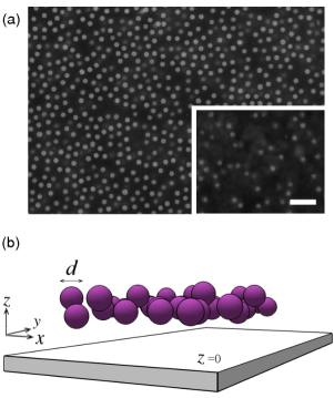
Figure 1: (a) Images of fluorescent $1.5\leavevmode\nobreak\ \mu$m-diameter silica spheres suspended in water, taken after the particles sedimented to create a quasi-2D suspension at area fraction $\phi=0.49$. Large (small) image corresponds to a typical image of the first (second) layer. Scale bar = $5\leavevmode\nobreak\ \mu$m. (b) Schematic view of the system and its parameters.

II.2 Imaging techniques

Particle position and motion in the $x$–$y$ plane, perpendicular to the optical axis, are observed using epifluorescence microscopy (Olympus IX71). Images are captured at a rate of $70$ fps by a CMOS camera (Gazelle, Point Grey Research). We use in-line holographic microscopy to image the dynamics of particles in three dimensions in dilute samples Kapfenberger et al. (2013). This imaging technique uses a collimated coherent light source (DPSS, Coherent, $\lambda=532$nm) to illuminate a sample mounted on a microscope. The light scattered from the sample interferes with the light passing through it, to form a hologram in the image plane. We reconstruct the light field passing through the sample by Rayleigh-Sommerfeld back-propagation and extract from it the particle location in three dimensions Lee and Grier (2007); Cheong et al. (2010); Kapfenberger et al. (2013). For holographic imaging measurements we use non-fluorescent silica particles with the same diameter ($d=1.50\leavevmode\nobreak\ \pm\leavevmode\nobreak\ 0.08\leavevmode\nobreak\ \mu$m, Polysciences Inc.). Additional details of the setup and measurement methods can be found elsewhere Kapfenberger et al. (2013).

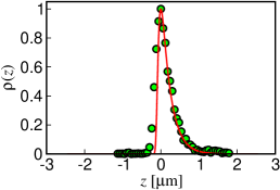
Figure 2: Holographic imaging. Height probability distribution of a single sphere (in salt-free water) shifted to the maximum value and fitted to the Boltzmann probability distribution (3) with the particle–wall potential (1).

We use confocal imaging to monitor particle positions in a dense layer in three dimensions. Our spinning disc confocal imaging system (Andor, Revolution XD) includes a Yokogawa (CSU-X1) spinning disc, and an Andor (iXon 897) EM-CCD camera. An objective lens (Olympus, x60, NA=1.1, water immersion) mounted on a piezoelectric scanner (Physik Instrumente, Pifoc P-721.LLQ) is used to scan the sample in the $z$ axis, with a step size of 100 nm.

II.3 Height calibration

A suspended tracer particle is subject to electrostatic and gravitational forces in addition to thermal fluctuations, affecting its height distribution Prieve (1999). The particle potential energy can be described as

$$U\leavevmode\nobreak\ =\leavevmode\nobreak\ mgz+B\mathrm{e}^{-(z-d/2)/\lambda},$$ (1)

where $z$ is the vertical position of the tracer, $g$ is the gravitational acceleration,

$$m=\textstyle\frac{\pi}{6}\Delta\varrho_{0}d^{3}$$ (2)

is the buoyant mass of the tracer ($\Delta\varrho_{0}$ is the mass density difference between silica and water), $\lambda$ is the Debye screening length, and the amplitude $B$ depends on $\lambda$ and the surface charges of both particle and glass surfaces. The corresponding probability distribution of the particle height $z$ is

$$\rho(z)=Z^{-1}\mathrm{e}^{-U(z)/k_{\rm B}T},$$ (3)

where $k_{\rm B}T$ is the thermal energy and $Z^{-1}$ is the normalization constant.

The height distribution of a single particle above the sample’s bottom was obtained from very dilute suspensions, using in-line holographic imaging Lee and Grier (2007); Cheong et al. (2010); Kapfenberger et al. (2013) (see Fig. 2). Our holographic measurements provide values of relative particle positions, but not the absolute particle heights with respect to the bottom wall. We thus set the peak position to $z=0$ and focus on the height relative to this reference plane. The exponential decay on the right side of the probability-density peak is governed by a decay length,

$$l=\frac{k_{B}T}{mg}$$ (4)

(the sedimentation length), resulting from the competition between gravity and thermal forces. The exponential-decay length determined from the holographic measurements agrees well with the calculated sedimentation length (4), without any fitting parameters (see Fig. 2). The electrostatic term of the probability-density, which controls the steep rise of the probability, affects mostly the peak position rather than its shape. Since we shifted the peak position to $z=0$, the fitting of the entire probability-density using Eqs. (1) and (3) was insensitive to the value of $B$. Reasonable fits were obtained for $\lambda$ in the range of $\lambda\sim 40-70$ nm. Better estimations of $B$ and $\lambda$ are given in Sec. IV.1.1, using mobility measurements.

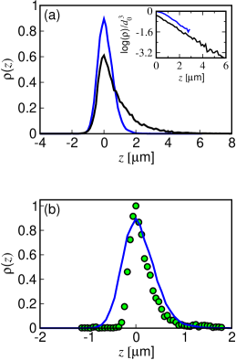
Figure 3: (a) Confocal imaging. Height probability distribution of silica particles at $\phi<0.003$ with diameters of $d_{0}=1.5\leavevmode\nobreak\ \mu$m (blue) and $d_{0}=1.0\leavevmode\nobreak\ \mu$m (black). Inset: Logarithm of the probability distributions scaled by $d_{0}^{3}$ in units of $10^{2}\leavevmode\nobreak\ \mu$m^-3; as expected, the two curves have approximately the same slope, which is used to calibrate the confocal height measurements. (b) Height probability distribution of silica particles with diameter $d_{0}=1.5\leavevmode\nobreak\ \mu$m extracted from holographic imaging (green circles, see Fig. 2) and confocal imaging (blue line). The suspensions in both figures were with no added salt, $[\textrm{KCl}]=0\,\textrm{M}$.

The applicability of the holographic imaging is limited to low-density suspensions, whereas the confocal imaging can be also used at higher concentrations. On the other hand, confocal height measurements suffer from spherical aberrations due to multiple changes in refractive index in the imaging path. This leads to a systematic error in measuring $z$, which can be eliminated by proper calibration. We calibrate the confocal measurement of the relative vertical particle positions by requiring the exponential decay of the height distribution to agree with the known, and verified, value of $l$.

In Fig. 3(a) we show the particle-height distribution $\rho(z)$ at $\phi<0.003$ for two different particle sizes ($d_{0}=1.0,1.5\leavevmode\nobreak\ \mu$m). The distributions are shifted so that the highest probability is located at $z=0$. Scaling the logarithm of the distributions by $d_{0}^{3}$ [inset of Fig. 3(a)] shows that the normalized decay constants for the two particle sizes have approximately the same value, from which we calibrate the confocal microscope’s height measurements. In Fig. 3(b), the height distributions extracted by the two methods (holographic and confocal imaging) are overlaid. This figure emphasizes the higher accuracy of holographic imaging over confocal imaging, especially around $z=0$, where the increase in distribution should be very steep Prieve (1999); Kapfenberger et al. (2013). The difference between the curves can also be attributed to polydispersity, since the holographic imaging is a single-particle measurement while the confocal imaging is a multiple-particle measurement, and its corresponding curve represents an average over $\sim$40 particles.

III Numerical methods

III.1 The system

III.1.1 Particles and their interactions

Silica particles are modeled as Brownian hard spheres with or without electrostatic repulsion (depending on the salt concentration), immersed in a fluid of viscosity $\eta$. The bottom wall is treated as an infinite hard planar surface. Creeping-flow conditions and no slip boundary conditions at the particle surfaces and at the wall are assumed.

In a salt solution with $[\textrm{KCl}]=0.01\,\textrm{M}$, the Debye length is only about 5 nm, and therefore electrostatic interactions are screened out. The particles thus interact only via infinite hard-core particle–particle and particle–wall potentials and the gravity potential $mgz$, and no other potential forces are involved. The strength of the gravity force is described by the sedimentation length (4).

In addition to the hard-core repulsion, in DDW with no added salt ($[\textrm{KCl}]=0\,\textrm{M}$) particles are assumed to also interact via particle–wall and particle–particle Debye–Hückel potentials,

$$V(z)=Be^{-(z-d/2)/\lambda},$$ (5)

and

$$V^{\prime}(r)=B^{\prime}e^{-(r-d)/\lambda},$$ (6)

where $\lambda$ is the Debye screening length, $B$ and $B^{\prime}$ are the potential amplitudes, and $r$ is the distance between the particle centers. The consideration of Debye–Hückel potentials in the salt-free case is based on our experimental measurement $\lambda\sim 60$ nm. A finite Debye screening length in DDW stems from the presence of residual ions in the solution Behrens and Grier (2001).

III.1.2 Suspension polydispersity

To determine the effects of the suspension polydispersity on the near-wall microstructure and dynamics, we have performed numerical simulations for a hard-sphere (HS) system with a Gaussian distribution of particle diameters,

$$p(d)=\frac{1}{(2\pi\sigma^{2})^{1/2}}\exp\left[-\frac{(d-d_{0})^{2}}{2\sigma^{2}}\right],$$ (7)

where $d$ and $d_{0}$ are the actual and average particle diameters, and $\sigma$ is the standard deviation. All the particles have the same mass density $\varrho_{0}$; hence, particles of different sizes have different buoyant masses and different sedimentation lengths (4). The dimensionless sedimentation length based on the average particle diameter $d_{0}$, is defined as

$$\frac{l_{0}}{d_{0}}=\frac{k_{B}T}{m_{0}gd_{0}},$$ (8)

where

$$m_{0}=\frac{\pi}{6}d_{0}^{3}\,\Delta\varrho_{0}.$$ (9)

The area fraction $\phi$ based on the average particle diameter $d_{0}$ is

$$\phi=\textstyle\frac{1}{4}\pi nd_{0}^{2},$$ (10)

where $n$ is the number of particles per unit area. Since the particles are free to move in the $z$ direction, the area fraction $\phi$ can exceed 1.

III.1.3 System parameters

The simulations were carried out for the following system parameters: For the dimensionless sedimentation length (8) we use the value

$$\frac{l_{0}}{d_{0}}=0.158,$$ (11)

calculated from the particle size and density. Based on the comparison between the calculated and measured values of the equilibrium average of the lateral self-diffusion coefficient for isolated particles in DDW, we estimate that the Debye length and the amplitude of particle–wall electrostatic repulsion are

$$\lambda/d=0.03,\qquad\frac{B}{k_{\rm B}T}=10.$$ (12)

These values are used for salt-free suspensions at all suspension concentrations. Assuming that the charge densities of the particle and wall surfaces are similar, we take

$$B^{\prime}=B/2,$$ (13)

for the interparticle-potential amplitude, as follows from the Derjaguin approximation Israelachvili (1992).

The simulations were performed in the range of area fractions $\phi\leq 1.2$. For polydisperse HS systems the calculations were carried out for $\sigma/d_{0}=0.10$, 0.15, 0.20, and 0.25 (we estimate that $0.10<\sigma/d_{0}<0.15$ for the silica particles used in the experiments). For particles interacting via the Debye–Hückel potentials (5) and (6) only monodisperse suspensions were considered.

III.2 Evaluation of the equilibrium distribution

III.2.1 Low density limit

For monodisperse suspensions at low particle concentrations, the equilibrium particle distribution $\rho(z)$ is given by the normalized Boltzmann factor (3). To determine the particle distribution for a dilute polydisperse suspension, the particle-size-dependent Boltzmann factor for individual particles, $\rho_{1}(z;d)$, is convoluted with the particle-size distribution (7),

$$\rho(z)=\int_{0}^{z}\textrm{d}d\,p(d)\rho_{1}(z;d),$$ (14)

For a HS system

$$\rho_{1}(z;d)=l^{-1}\textrm{e}^{-(z-d/2)/l}\theta(z-d/2),$$ (15)

according to equations (1)–(4), where $\theta(x)$ is the Heaviside step function, and the sedimentation length $l$ is particle-size dependent due to the variation of particle mass.

III.2.2 Monte–Carlo simulations

To determine the equilibrium microstructure of a sedimented suspension at finite particle area fractions, equilibrium Monte–Carlo (MC) simulations were performed for 2D-periodic arrays of spherical particles in 3D space (with periodicity in the horizontal directions $x$ and $y$ and the box size $L$). The particles interact via infinite hard-core repulsion and the pair-additive potential

$$U(\bm{X)}=\sum_{i=1}^{N}m_{i}gz_{i}+\sum_{i=1}^{N}V(z_{i})+\frac{1}{2}\sum_{i=1}^{N}\sum_{j\neq i}^{N}V^{\prime}(r_{ij}),$$ (16)

which includes the gravity term and particle–wall and particle–particle screened electrostatic potentials (5) and (6). Here $\bm{X}=(\mathbf{r}_{1},\ldots,\mathbf{r}_{N})$ is the particle configuration (with $\mathbf{r}_{i}$ denoting the position of particle $i$), $z_{i}$ is the vertical coordinate of particle $i$, and $r_{ij}=|\mathbf{r}_{i}-\mathbf{r}_{j}|$ is the relative particle distance.

A purely HS system with $V=V^{\prime}=0$ was modeled for monodisperse particles and for polydisperse particles with the Gaussian size distribution (7). For systems with nonzero electrostatic repulsion only monodisperse particles were considered.

The initial configuration was prepared by placing $N=400$ particles randomly in a vertical cuboid box with the square base $L$ and the height $10L$. The size $L$ of the 2D-periodic cell was determined to obtain the required area fraction $\phi$ of the sedimented particle layer. The suspension was allowed to sediment by following the MC random-walk dynamics in the configurational space $\bm{X}$ Frenkel and Smit (2002) (as described below). After the equilibrium state was reached, suspension properties were obtained by averaging the quantities of interest over at least 200 independent configurations.

Our adaptive simulation procedure was performed by repeating the MC steps defined as follows:

• A randomly selected particle $i$ is given a small random displacement, $\bm{r}_{i}\rightarrow\bm{r}_{i}^{\prime}=\bm{r}_{i}+\bm{\Delta}$, where $\bm{\Delta}$ is chosen from a 3D Gaussian distribution with the standard deviation adaptively adjusted to the current mean gap between particles. This displacement results in the change of the configuration from $\bm{X}$ to $\bm{X}^{\prime}$.

• According to the Metropolis detailed balance condition, the new configuration is accepted with the probability

  $$\min\left(1,\exp\left\{-\left[U(\bm{X}^{\prime})-U(\bm{X})\right]/k_{B}T\right\}\right),$$ (17)

  provided that there is no particle–particle or particle–wall overlap.

To let the system reach an equilibrium state $\bm{X}_{1}$, the MC step (a) and (b) is repeated $10^{5}N$ times. The next independent equilibrium configuration $\bm{X}_{n+1}$ is obtained from the previous configuration $\bm{X}_{n}$ by performing $10^{4}N$ MC steps. The particle height distribution $\rho(z)$ and other equilibrium quantities are obtained by averaging over 200 independent configurations $\bm{X}_{i}$.

III.3 Hydrodynamics and self-diffusion

III.3.1 Low density limit

In the absence of a wall, the self-diffusion coefficient of an isolated solid sphere with diameter $d_{0}$ is given by the Stokes–Einstein expression

$$D_{0}=\frac{k_{\rm B}T}{3\pi\eta d_{0}}.$$ (18)

The self-diffusion coefficient $D(z)$ of a sphere with diameter $d$ at a distance $z$ from the wall is smaller by a factor

$$\frac{D(z)}{D_{0}}=\frac{d_{0}}{d}\,\mu_{\parallel}(z/d),$$ (19)

where the normalized mobility coefficient $\mu_{\parallel}$ depends on the dimensionless particle position $z/d$ and no other parameters. Relation (19) refers to the lateral component of the self-diffusion coefficient (parallel to the wall), which was measured in our experiments. However, an analogous expression also holds for the normal component.

For monodisperse particles in the dilute-suspension limit, the effective self-diffusion coefficient $D_{s}$ averaged across the suspension layer is obtained by integrating (19) with the Boltzmann distribution (3),

$$\frac{D_{s}}{D_{0}}=\int_{d/2}^{\infty}\textrm{d}z\,\rho(z)\mu_{\parallel}(z/d).$$ (20)

For a polydisperse suspension, an additional average over the particle-size distribution (7) is needed,

$$\frac{D_{s}}{D_{0}}=\int_{0}^{\infty}\textrm{d}d\,p(d)\int_{d/2}^{\infty}\textrm{d}z\,\rho_{1}(z;d)\mu_{\parallel}(z/d).$$ (21)

The mobility coefficient $\mu_{\parallel}(z/d)$ was evaluated with high accuracy using the Hydromultipole algorithm for a particle near a single wall Cichocki and Jones (1998). The integrals in Eqs. (20) and (21) were performed numerically using the Gauss method, with $\mu_{\parallel}(z/d)$ calculated by a series expansion.

III.3.2 Computations for larger densities

The effective self-diffusion coefficient for suspensions at higher concentrations was evaluated using a periodic version Bławzdziewicz and Wajnryb (2008) of the Cartesian-representation algorithm for a system of particles in a parallel-wall channel Bhattacharya et al. (2005b, c). In our approach, periodic boundary conditions in the lateral directions are incorporated by splitting the flow reflected by the particles into a short-range near-field contribution and a long-range asymptotic Hele–Shaw component. The near-field contribution is summed explicitly over neighboring periodic cells, and the Hele–Shaw component is evaluated using Ewald summation method for a 2D harmonic potential Cichocki and Felderhof (1989); Bławzdziewicz and Wajnryb (2008).

The one-wall results were derived from the two-wall calculations using an asymptotic procedure based on the observation that in the particle-free part of the channel the velocity field tends to a combination of a plug flow and a shear flow. All other flow components decay exponentially with the distance from the particle layer. The one-wall results are obtained by eliminating the shear flow and retaining only the plug flow generated by hydrodynamic forces induced on the particles Sadlej et al. (2009). The calculations were performed for the distance to the upper virtual wall $H=10d_{0}$, which is sufficient to obtain highly accurate one-wall results.

The self-diffusion coefficient is determined by averaging the trace of the lateral translational–translational $N$-particle mobility, evaluated using Hydromultipole codes based on the above algorithm, with the multipole truncation order $L=2$ Abade et al. (2010). The averaging was performed over equilibrium configurations of $N=400$ particles in a 2D-periodically replicated simulation cell. Independent equilibrium configurations were constructed using the MC technique described in Sec. III.2.2.

IV Structure of the quasi-2D suspensions

IV.1 Experimental results

A typical image of our quasi-2D colloidal suspension is shown in Fig. 1. For each area fraction $\phi$ and salt concentration, the suspension can be characterized by the structure in the $x$–$y$ plane (parallel to the cell floor) and the density profile in the $z$ direction (perpendicular to the floor). In this section we discuss results of our measurements of the microstructure of a sedimented particle layer.

IV.1.1 Mean particle height at low area fractions

As mentioned in Sec. II.3, our imaging techniques do not yield absolute particle heights. To estimate the mean particle distance $z$ from the bottom wall (the mean height) in a dilute suspension layer, we observe particle dynamics in the horizontal directions, and compare measurement results with theoretical calculations of the effect of the wall on the lateral particle diffusion. Using fluorescence imaging, we determine the projection of particle trajectories onto the $x$–$y$ plane, $\mathbf{r}_{\parallel}(t)$, and extract the effective self-diffusion coefficient,

$$D_{s}=\langle\Delta\textbf{r}_{\parallel}^{2}(\tau)\rangle/(4\tau),$$ (22)

where $\tau$ is the time interval. The position-dependent diffusivity $D(z)$ in the $x$–$y$ plane of a single particle near a planar wall is given by the following expansion in the particle–wall distance Happel and Brenner (1983); Perkins and Jones (1992),

$$\frac{D(z)}{D_{0}}=1 - \frac{9}{32}\frac{d}{z}+\frac{1}{64}\left(\frac{d}{z}\right)^{3}$$

$$- \frac{45}{4096}\left(\frac{d}{z}\right)^{4}-\frac{1}{512}\left(\frac{d}{z}\right)^{5},$$

where $z=0$ is the wall position. The expansion (IV.1.1) is accurate within 5% to 1% as $z$ increases from $0.51d$ up to $d/2+2l$, in the range where sedimented particles spend most of the time in a low-density suspension under equilibrium conditions. Here $l\approx 0.16d$ is the sedimentation length (4).

From expression (IV.1.1) and $D_{s}$ extracted according to (22), we can calculate the suspension’s mean distance from the wall (where $z$ in (IV.1.1) is replaced by a mean value $\langle z\rangle$). This calculation holds in the limit $\phi\to 0$, where there are no particle-particle interactions. We measure $D_{s}$ from the particle trajectories, $\mathbf{r}_{\parallel}(t)$, in extremely low area fraction solution, $\phi<0.003$ (in salt-free water), and obtain a mean distance from the wall $\langle z\rangle=1.1\pm 0.1\,\mu$m, corresponding to a mean gap $\epsilon=z-d/2$ of 0.3–0.4 $\mu$m between the particle surface and the wall. We also extract $\langle z\rangle$ for different salt concentrations by extrapolating $D_{s}$ (measured at various area fractions) to $\phi=0$ (see Sec. V.1), obtaining $\langle z\rangle=0.95\pm 0.05\,\mu$m for $[\textrm{KCl}]=0.01\,\textrm{M}$ and $\langle z\rangle=1.11\pm 0.05\,\mu$m for $[\textrm{KCl}]=0\,\textrm{M}$. The latter matches the average height extracted from the diffusion of tracers in the extremely low density suspension.

For $\lambda=5$ nm (added salt), the mean height calculated from the Boltzmann distribution (3) is dominated by the exponential decay due to gravity and is practically independent of $B$ in the particle–wall potential (1). For $B=0$, using the particle mass as determined from Eq. (2) with no fitting parameters, we get $\langle z\rangle=0.99$ $\mu$m, in agreement with the diffusivity-based measurements of $\langle z\rangle$. This result confirms that in the added-salt case we can neglect the electrostatic repulsion from the wall. For the salt-free case, taking $\lambda=50$ nm, we obtain $\langle z\rangle=1.11$ $\mu$m for $B$ in the range 5–15 $k_{\rm B}T$. These values are consistent with those obtained by fitting the measured height distribution to the theoretical expression (1) (see Sec. II.3).

Since Eq. (IV.1.1) does not include lubrication correction for small particle–wall gaps $\epsilon$, it overpredicts $D(z)$ for $z<0.51d$; however, the accuracy of the approximation is sufficient for the purpose of the present estimates. In our calculations discussed in Secs. III and V.2, highly accurate Hydromultipole results were used instead of the far-field approximation (IV.1.1).

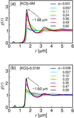
Figure 4: Radial distribution function $g(r)$ in the $x$–$y$ plane for experiments in (a) salt-free and (b) salt-added ($[\textrm{KCl}]=0.01\,\textrm{M}$) water. The distribution $g(r)$ was calculated separately in the first and second layers (see Sec. IV.1.4 for the layer definition) and combined with appropriate weights.

IV.1.2 Radial distribution in the horizontal plane

To verify that no crystalline or hexatic structures are formed at higher values of the area fraction, we evaluate from the experiment the radial distribution function $g(r)$ and the full 2D pair distribution $g(r,\theta)$ in the $x$–$y$ plane, for both the salt-free and salt-added suspensions. No dependence on $\theta$ was found. The radial distribution $g(r)$ for several values of the area fraction $\phi$ is shown in Fig. 4(a) for the salt-free system and in 4(b) for the salt-added system.

For monodisperse hard spheres the first peak of $g(r)$ should correspond to the diameter of the sphere. Our measurements show that the first peak is at $r=1.68\leavevmode\nobreak\ \mu$m for suspensions without salt and at $r=1.60\leavevmode\nobreak\ \mu$m for suspensions with $[\textrm{KCl}]=0.01\,\textrm{M}$. The difference between these two numbers implies that the effective shell around the particles in the salt-free samples is around  40-50 nm, which provides an estimation for the screening length in DDW without the addition of salt. This estimate of $\lambda$ is consistent with the other two mentioned above.

IV.1.3 Vertical density profile

The height distributions $\rho(z)$ of the silica particles at different area fractions of the sedimented particle layer were acquired using confocal imaging and conventional image analysis Crocker and Grier (1996). These distributions for salt-added suspensions with $[\textrm{KCl}]=0.01\,\textrm{M}$ are plotted in Fig. 5(a) for several values of the area-fraction $\phi$. Since we cannot precisely measure the position of the wall, the distributions are shifted so that their first peak (close to the wall) is located at $z=0$. These distributions indicate the formation of a second layer of particles for area fractions $\phi\gtrsim 0.26$. The observed center of the second layer is located $\Delta z\approx 0.75\,\mu$m above the center of the first layer. The layer separation is thus significantly smaller than the expected separation $\Delta z\approx d=1.5\,\mu$m (which is similar to the peak separation for the radial distribution). See further discussion in Secs. VI and Appendix A.

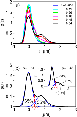
Figure 5: (a) Height probability distribution of the silica colloids (in $[\textrm{KCl}]=0.01\,\textrm{M}$) for increasing area fraction reveals the formation of a second layer. Colors correspond to different area fractions (as labeled). (b) For the most dense suspensions [$\phi=0.54$ and $\phi=0.48$ (inset)], the height distribution (black solid line) around the two peaks can be fitted to two Gaussian functions (blue lines). The intersection of the two Gaussians defines an effective boundary (red broken line) between the first and second layers; occupation percentages are indicated.

To highlight the onset of the formation of the second layer, we look at the subtraction of the height probability distribution of the lowest area fraction from the distribution of all area fractions, $\Delta\rho\equiv\rho-\rho_{\,\phi=0.054}$ [Fig. 6(a)]. Two phenomena are expected when a second layer is formed: (i) negative values at $z=0\leavevmode\nobreak\ \mu$m, corresponding to a reduction in the fraction of particles populating the first layer, (ii) positive and increasing values at $z=0.75\leavevmode\nobreak\ \mu$m, corresponding to the formation and increasing population of the second layer. The values of $\Delta\rho$ at $z=0$ and $0.75\leavevmode\nobreak\ \mu$m are plotted in Fig. 6(b). The two expected phenomena are observed at approximately $\phi\sim 0.3$, indicating the area fraction above which a second layer becomes occupied. At area fractions smaller than 0.3 we still obtain negative values of $\Delta\rho$ at $z=0\leavevmode\nobreak\ \mu$m, and positive values at $z=0.75\leavevmode\nobreak\ \mu$m, however these values are relatively low and can correspond to the broadening of the exponential distribution due to increase in $\phi$.

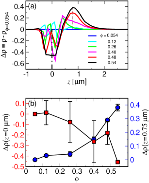
Figure 6: (a) The difference between the height probability distribution at increasing area fractions and the distribution at the lowest area fraction $\phi=0.054$, $\Delta\rho\equiv\rho-\rho_{\,\phi=0.054}$ (in $[\textrm{KCl}]=0.01\,\textrm{M}$). Colors are as in Fig 5(a). Gray (black) dashed line corresponds to $z=0.75\leavevmode\nobreak\ \mu$m ($z=0\leavevmode\nobreak\ \mu$m). (b) Values of $\Delta\rho$ at $z=0\leavevmode\nobreak\ \mu$m (red squares) and $z=0.75\leavevmode\nobreak\ \mu$m (blue circles) for all area fractions. Both plots exhibit a change in trend at area fraction $\phi\sim 0.3$.

IV.1.4 Particle-layer occupation fractions

For the area fractions at which a clear second peak in the particle distribution $\rho$ is seen in Fig. 5(a) (i.e., for $\phi=0.48$ and $0.54$), we fit the area around each peak to a Gaussian function and define the point of intersection between the two Gaussians as the effective boundary between the two layers. Figure 5(b) shows the two distributions with the Gaussian fits and our definition of that boundary, which turns out to be at a distance of $0.39\pm 0.04\leavevmode\nobreak\ \mu$m above the peak of the first layer in both densities.

Using this boundary, we evaluated the occupation fractions $f_{i}=\phi_{i}/\phi$ of the bottom ($i=1$) and top layer ($i=2$), where $\phi_{i}$ is the area fraction of particles in layer $i$. The results are shown in Fig. 7(a) for a suspension in $[\textrm{KCl}]=0.01\,\textrm{M}$ solution as a function of the total area fraction $\phi$. As expected, the fraction of particles populating the second layer grows as the total area fraction of the suspension is increased.

An additional independent measurement of the layer occupation fractions is done using epifluorescence microscopy, which enables us to image the different layers separately [see Fig. 1(a)]. The occupation fraction of each layer is determined by counting the number of particles observed therein. The occupation fractions measured using the epifluorescence imaging technique are plotted in Fig. 7(a) along with the results obtained from the confocal microscopy. The two methods yield similar results.

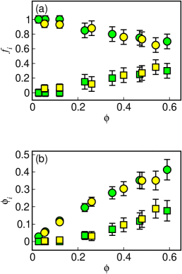
Figure 7: Occupation fractions $f_{i}$ and area fractions $\phi_{i}$ of suspension layers as a function of the total area fraction $\phi$; circles (squares) correspond to the first (second) layer. (a) Occupation fractions for experiments in $[\textrm{KCl}]=0.01\,\textrm{M}$ extracted from the confocal height distribution curves (yellow) and from the 2D images (green), showing good agreement between the two methods. (b) The same data replotted for the area fractions $\phi_{1}$ and $\phi_{2}$ of the first and second layers.

Alternatively, we can represent the layer-occupation results in terms of the area fractions $\phi_{1}$ and $\phi_{2}$ of the first and second layers [see Fig. 7(b)]. Both $\phi_{1}$ and $\phi_{2}$ increase as $\phi$ is increased, and $\phi_{1}$ seems to saturate at $\phi>0.45$.

IV.2 Numerical simulations

Figure 8: Particle–wall distribution function for (a) monodisperse suspension; (b) polydisperse suspension with standard deviation of particle diameter $\sigma/d_{0}=0.15$. Simulation results for area fraction $\phi=0$ (solid line), 0.3 (dashed), 0.6 (dotted), 0.9 (dot–dashed), 1.2 (long-dashed). The insets show the deviation $\Delta\rho=\rho-\rho_{\phi=0}$ from the low-density distribution.

Figure 9: Particle–wall distribution function for area fractions (a) $\phi=0.054$ and (b) $0.54$. Experimental results (solid circles); simulation results for standard deviation of particle diameter $\sigma/d_{0}=0$ (solid line), $0.1$ (dashed), $0.15$ (dotted), $0.20$ (dashed–dotted), and $0.25$ (long-dashed).

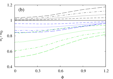
Figure 10: (a) Occupation fraction $f_{i}$ and (b) normalized average particle diameter $d_{i}$ in the first particle layer (black), second layer (blue), and third layer (green), vs the total area fraction $\phi$. The results for a monodisperse system (solid lines) and polydisperse systems with standard deviation of particle diameter $\sigma/d_{0}=0.1$ (dashed), $0.15$ (dotted) $0.20$ (dash–dotted), and $0.25$ (long-dashed). The symbols represent experimental results from confocal imaging (circles) and 2D images (squares) for a suspension with salt concentration $[\textrm{KCl}]=0.01\,\textrm{M}$. Note that the experimental second layer corresponds to the sum of the second and third layers in the MC simulations. The layer boundaries in the numerical calculations are set at $z_{1}=0.9d_{0}$, and $z_{2}=1.8d_{0}$ and in the experiments are obtained from Gaussian fitting (see Fig. 5).

Figure 11: Low-density limit of the near-wall particle distribution for a monodisperse system (solid line) and polydisperse systems with standard deviation of particle diameter $\sigma/d_{0}=0.1$ (dashed), $0.15$ (dotted) $0.20$ (dash–dotted), and $0.25$ (long-dashed).

Here we present results of MC simulations of the equilibrium microstructure of a HS suspension in the near wall region. The HS potential corresponds to the system with $[\textrm{KCl}]=0.01\,\textrm{M}$, for which the electrostatic repulsion is negligible. Since the suspension used in the experiments is polydisperse, we consider both monodisperse and polydisperse systems.

IV.2.1 Near-wall particle distribution

Figure 8 shows MC results for the suspension density profile $\rho(z)$ for a monodisperse suspension and polydisperse suspensions at several area fractions. Similarly to the experimental results, the simulations show that there is a single layer of sedimented particles at low area fractions $\phi$, and a two-layer microstructure at higher area fractions. (Development of a third layer for $\phi\gtrsim 0.9$ is also noticeable in the region $z/d_{0}\gtrsim 2$.) Suspension polydispersity results in broadening of the peaks of the particle distribution.

A direct comparison between the experimental and simulation results is presented in Fig. 9 for two values of the area fraction $\phi$. At low area fractions [Fig. 9(a)] the agreement between the experiments and simulations is good. (The standard deviation of the particle-size distribution for which the simulations match the experimental data, $\sigma/d_{0}\approx 0.25$, is larger than the estimated standard deviation $0.1<\sigma/d_{0}<0.15$ based on the manufacturer’s specifications; the additional spread of the experimentally observed peak can be attributed to random errors of the particle height evaluation from the confocal-microscopy images.)

A comparison of the numerical and experimental results at a higher area fraction, as shown in Fig. 9(b) [also see Figs. 5 and 8], reveals that (i) the experimentally observed second maximum of the density distribution develops at lower area fractions than the corresponding maximum in the numerical simulations; (ii) the experimental second peak is narrower, and its position is shifted towards the wall. In contrast, the plots of the excess distribution $\Delta\rho$ with respect to the low-density limit, shown in Fig. 6(a) and the insets of Fig. 8, indicate that the onset of the formation of the second layer occurs at approximately the same area fraction according to the simulations and experiments. Moreover, the measured and calculated occupation fractions of the layers are similar for all area fractions, as depicted in Fig. 10(a). A possible source of the observed discrepancies between the experimental and numerical results for the particle distribution $\rho(z)$ is described in Appendix A. It also provides a plausible explanation of the fact that the agreement between the experiments and MC simulations for the layer occupation fractions $f_{i}$ is quite good in spite of the discrepancies for $\rho(z)$.

IV.2.2 Polydispersity effects

The results in Fig. 10(a) show that the occupation fraction of the first two layers is relatively insensitive to the suspension polydispersity; in contrast, the occupation fraction of the third layer strongly increases with the standard deviation of particle diameter. This increase stems from the presence of smaller (lighter) particles in polydisperse systems: smaller particles tend to migrate into the top layer, as evident from Fig. 10(b). For dilute suspensions, the particle-size segregation results in variation of the slope of $\log\rho(z)$ with the distance from the wall, as illustrated in Fig. 11. We estimate that this variation causes an approximately 20 % uncertainty of the calibration of the confocal height measurements described in Sec. II.3.

IV.3 A quasi-2D model of the equilibrium layered microstructure

Here we present a semi-quantitative theoretical model for evaluating the occupation fractions $f_{i}$ of the particle layers in a sedimented colloidal suspension. Our theory is based on the assumption that the suspension microstructure can be approximated as a collection of weakly coupled quasi-2D layers in thermodynamic equilibrium with respect to particle exchange.

The equilibrium condition for layers $i$ and $i+1$ is

$$\mu_{i}+mgz_{i}=\mu_{i+1}+mgz_{i+1},$$ (24)

where $\mu_{i}$ is the chemical potential of layer $i$, and $z_{i}$ is its position. In our model, $\mu_{i}$ is approximated as the chemical potential of a 2D hard-disk fluid of area fraction $\phi_{i}$. All disk diameters are equal to the sphere diameter $d$, which corresponds to a layer of spheres with the same vertical position $z$.

In the low area-fraction limit, the chemical potential of a hard-disk fluid is

$$\mu_{i}=k_{\rm B}T\ln\phi_{i}+C(T),$$ (25)

where $C(T)$ depends only on the temperature $T$. According to the equilibrium condition (24) and equation of state (25), we thus have

$$\phi_{i+1}=r\phi_{i},\qquad i=1,2,\ldots$$ (26)

with the ratio $r$ given by the Boltzmann factor

$$r=\textrm{e}^{-\Delta/l},$$ (27)

where $l$ is defined by Eq. (4) and $\Delta=z_{i+1}-z_{i}$. We assume that the layer separation $\Delta$ is independent of $i$.

For finite area fractions, relation (26) is replaced with

$$\phi_{i+1}=r(\phi_{i})\phi_{i},\qquad i=1,2\ldots,$$ (28)

where the layer occupation ratio $r$ depends on the area fraction in the adjacent layers. The factor $r(\phi)$ is determined from the equilibrium condition (24) with the help of the Gibbs–Duhem relation

$$\textrm{d}\mu=\frac{\pi d^{2}}{4}\phi^{-1}\textrm{d}p,$$ (29)

where $p$ is the lateral 2D pressure within the layer. Combining (24), (28), and (29) yields

$$\frac{\textrm{d}r}{\textrm{d}\phi}=r\left[\frac{p^{\prime}(\phi)}{p^{\prime}(r\phi)}-1\right],$$ (30)

where

$$p^{\prime}=\left(\frac{\partial p}{\partial\phi}\right)_{T}.$$ (31)

The differential equation (30) is solved for $r=r(\phi)$ with the boundary condition (27) at $\phi=0$. Occupation fractions $f_{i}=\phi_{i}/\phi$ are then determined by iteration, applying Eq. (28) and the relation

$$\phi=\sum_{i=1}^{\infty}\phi_{i}.$$ (32)

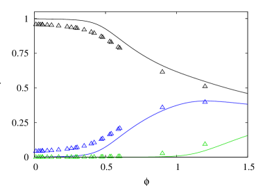
Figure 12: Occupation fraction $f_{i}$ for the first (black), second (blue) and third (green) layer vs the total area fraction $\phi$ for a monodisperse HS suspension. Theoretical results (solid lines); MC simulations (symbols).

We have solved Eq. (30) and determined the occupation fractions $f_{i}$ using the scaled-particle-theory equation of state for hard disks Helfand et al. (1961),

$$\frac{\pi d^{2}p}{4k_{\rm B}T}=\frac{\phi}{(1-\phi)^{2}}.$$ (33)

The results of our calculations are presented in Fig. 12 for a HS system with the same value of the sedimentation length (11) as in our MC simulations. Based on the separation between the first and second peak of the suspension density profile shown in Fig. 8(a), the calculations were performed for $\Delta/d=1$.

The theoretical results in Fig. 12 are compared with the MC simulations of a monodisperse HS suspension with the boundaries between the layers set to $z_{1}=d$ and $z_{2}=2d$, consistent with the peak positions. The agreement between our simple theory and simulations is quite good. A similar agreement was obtained for other values of the dimensional parameter $l/d$ (results not shown).

The layer boundaries used in Sec. IV.2 and V.2 to compare the MC results with experiments differ from the boundaries used in the above model by approximately 10 %. Due to the observed deviation between the measured and simulated particle distributions (see Fig. 9), it is not possible to define the layer boundaries in a unique, equivalent way for the experimental and simulated systems. Therefore, the layer boundaries $z_{1}=0.9d$ and $z_{2}=1.8d$ used in Sec. IV.2 and V.2 were chosen based on the comparison between the experimental and numerical results for the occupation fractions and self-diffusivities in particle layers.

V Particle dynamics

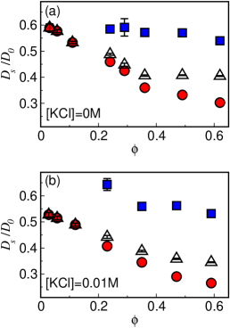
Figure 13: Short-time self-diffusion coefficient $D_{s}$, normalized by the Stokes-Einstein diffusion coefficient $D_{0}$, as a function of the total area fraction $\phi$; circles (squares) correspond to the first (second) layer, and triangles to the effective $D_{s}$ calculated by the weighted average of the self-diffusion coefficients for the two individual layers. (a) Suspension with no added salt. (b) Suspension with salt concentration $[\textrm{KCl}]=0.01\,\textrm{M}$.

V.1 Experimental results

The short time self-diffusion coefficient in the $x$–$y$ plane, $D_{s}$, is determined for different total area fractions of the sedimented particles by extracting the mean square displacement (22) from 2D epifluorescent images of the first and second particle layer. The mean-square displacement is measured over a time interval $\tau$ that is small compared to the structural relaxation time of the suspension, to ensure that the measurements yield the short-time self-diffusion coefficient.

The results are shown in Fig. 13 for suspensions with salt concentration $[\textrm{KCl}]=0.01\,\textrm{M}$ and salt-free suspensions with $[\textrm{KCl}]=0\,\textrm{M}$. The self-diffusion coefficient is expected to decrease as the particle concentration increases; indeed, we observe this decrease for both salt concentrations and in both layers, for $\phi<0.4$. In the case of $[\textrm{KCl}]=0.01\,\textrm{M}$, corresponding to $\lambda=5$ nm, the particles can get much closer to the cell floor, which in turn results in lower values of the self-diffusion coefficient compared to suspensions with $[\textrm{KCl}]=0\,\textrm{M}$.

Using a linear fit to the values of $D_{s}/D_{0}$ for the low area fractions, where there is no observable second layer, we can extrapolate to $\phi=0$ and extract the self-diffusivity of a single particle. The extrapolated results agree well with the measurements at very low concentrations $\phi<0.003$, as discussed in Sec. IV.1.1.

From the known occupation fractions $f_{1}$ and $f_{2}$ for each $\phi$ we can weigh the contribution of each layer to the total self-diffusivity, and construct an effective $D_{s}$ of the whole suspension (Fig. 13). As expected, for $\phi<0.4$ the effective self-diffusion coefficient $D_{s}$ decreases as $\phi$ is increased in both salt concentrations. For larger $\phi$ we observe a flattening of $D_{s}$, which clearly indicates that the second layer becomes dominant in those area fractions. This observation is supported also by the saturation of $\phi_{1}$ at $\phi>0.45$ [Fig. 7(b)].

V.2 Numerical simulations

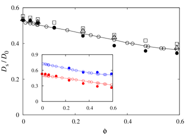
Figure 14: Normalized short-time self-diffusion coefficient $D_{s}/D_{0}$, as a function of the area fraction $\phi$ for a suspension with salt concentration $[\textrm{KCl}]=0.01\,\textrm{M}$. The main panel shows $D_{s}$ averaged over the whole system, and the inset shows $D_{s}$ for the first (bottom, red) and second (top, blue) particle layer. Experimental results (solid circles); simulation results (open symbols) for a monodisperse system (circles) and polydisperse systems with the standard deviation of the particle diameter $\sigma=0.1d_{0}$ (triangles) and $0.15d_{0}$ (squares). Note that at low area fractions the triangles overlap with the solid circles. The lines are a guide for the eye.

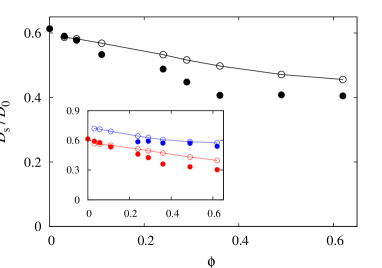
Figure 15: Normalized short-time self-diffusion coefficient $D_{s}/D_{0}$, as a function of the area fraction $\phi$ for a suspension with no salt. Symbols are the same as in Fig. 14. Results are shown only for monodisperse suspensions.

Figure 16: Normalized short-time self-diffusion coefficient $D_{s}/D_{0}$ in the low-area-fraction limit $\phi=0$ (for the system with salt) as a function of the suspension polydispersity.

The results of our numerical simulations for the short-time lateral self-diffusion coefficient $D_{s}$ in a HS system are presented in Fig. 14 for a monodisperse suspension and for polydisperse suspensions with $\sigma/d_{0}=0.1$ and $0.15$. Figure 15 shows the corresponding results for a system of monodisperse hard spheres with particle–wall and particle–particle electrostatic repulsion (5) and (6).

The results depicted in Fig. 14 indicate that for moderately polydisperse suspensions (in the range corresponding to the polydispersity of silica particles used in the experiments), the self-diffusion coefficient is only moderately dependent on $\sigma/d_{0}$. For larger values of the variance of particle diameters, the normalized self-diffusion coefficient $D_{s}/D_{0}$ significantly increases with the degree of the polydispersity, because the mobility is dominated by small particles. This increase is illustrated in Fig. 16 for a suspension in the low-area-fraction limit $\phi=0$.

The results of our hydrodynamic calculations for a HS suspension and for a suspension with screened electrostatic repulsion are compared with experimental results for suspensions with $[\textrm{KCl}]=0.01\,\textrm{M}$ (Fig. 14) and $[\textrm{KCl}]=0\,\textrm{M}$ (Fig. 15). For the system with salt, the measured values are slightly closer to their numerical analogs than in the absence of salt. Summarizing, the experimental and numerical results agree well both for the overall self-diffusivity and for the self-diffusivity in individual particle layers.

VI Discussion

In this paper we have studied in detail the structure and dynamics of quasi-2D colloidal suspensions near a wall, comparing experiment and theory. Our central result is a rather sharp formation of a distinct second layer at an area fraction of $\phi\sim 0.3$. This value is much lower than the area fraction required for close-packing or other 2D structural changes such as the formation of hexatic or crystalline order. One important consequence of this result concerns the apparent self-diffusion of the particles in the suspension and its dependence on particle density. Due to the higher mobility of the particles in the elevated layer, the effective diffusivity is higher and levels off as particle density increases. The experimentally observed behavior could be interpreted incorrectly if one is unaware of the layering (or stratifying) effect.

We find good agreement between experimental and simulation results for the occupation fractions of the first and second layers and for the lateral self-diffusivity (both for the entire suspension and in the individual layers). However, we also find an unexpected discrepancy in the position and the height of the second peak in the near-wall particle distribution. While the source of this discrepancy is unknown, one possibility, related to optical aberrations, is suggested in Appendix A. On the other hand, the difference between theory and experiment might also be a result of an actual physical effect, such as more complicated electrostatic interactions setting in at higher layer densities.

Another new insight put forth in this study is the significant effect that polydispersity has on the occupation and composition of layers close to the bottom wall, even in the case of a relatively small dispersion of particle sizes. The effect of polydispersity is evident already at low densities, since the smaller and larger particles segregate into the upper and lower layers, respectively. We expect the phenomena described here to be quite general and to be manifested in any such system where the sedimentation length $l$ is of the order of the particle diameter. This conclusion is supported by the appearance of the phenomena both in experiments and in Monte–Carlo simulations.

An important outcome of this paper is the construction of a very simple theoretical quasi-2D model of the layered microstructure in thermodynamic equilibrium. Such systems have been analyzed earlier using density-functional theory Chen and Ma (2006), but our theoretical model is much simpler and easier to apply. We have demonstrated that the model approximates well the experimental and numerical results for the system studied in this work.

We conclude with three open issues. Layering phenomena near a wall are well documented in 3D suspensions as well Van Winkle and Murray (1988); González-Mozuelos et al. (1991); Zurita-Gotor et al. (2012). An interesting question is whether this perturbation to the 3D pair correlation function could be fundamentally related to the sequential layering reported here. The structural features near the wall should also affect two- and many-particle dynamics in the quasi-2D suspensions, which can be characterized by two-point microrheology. Finally, taking a more detailed account of interparticle forces such as strong electrostatic interactions may hopefully provide deeper understanding of the effects observed in this work.

Appendix A

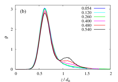
Figure 17: The effect of the model distortion transformation (36) on the particle distribution $\rho(z)$ in a HS suspension with the standard deviation of the particle distribution $\sigma/d_{0}=0.2$. (a) A comparison of the MC result for $\rho(z)$ (solid line) with the transformed distribution (35) (dashed line) at the area fraction $\phi=0.54$; (b) the transformed distribution for different area fractions (as labeled). The parameters of the transformation (36) are $z_{1}/d=0.55$, $z_{2}/d=1.2$, and $\alpha=2.5$.

We present a simple model to support a hypothesis that the discrepancy between the measured and calculated near-wall particle distributions stems from optical aberration caused by nonuniform optical properties of the suspension in the near-wall region. We assume that such aberration produces a nonlinear rescaling of the coordinate $z$,

$$\tilde{z}=\tilde{z}(z),$$ (34)

where $z$ is the actual and $\tilde{z}$ is the measured particle position. The rescaling (34) results in the corresponding transformation of the particle density

$$\tilde{\rho}(\tilde{z})=\rho(z)\frac{d\,z}{d\,\tilde{z}}.$$ (35)

To demonstrate that a distortion (34) can produce the observed shift and change of height of the features of the distribution $\rho$, we consider an ad hoc distortion model with the transformation between the measured and actual vertical coordinates given by the equations

$$\frac{d\,\tilde{z}}{d\,z}=\left\{\begin{array}[]{ll}1;&z<z_{1},\\ 1-(1-b)\displaystyle\frac{z-z_{1}}{z_{2}-z_{1}};&z_{1}\leq z\leq z_{2},\\ b;&z_{2}<z,\end{array}\right.$$ (36a)

and

$$b=\alpha\phi,$$ (36b)

where $z_{1}$, $z_{2}$, and $\alpha$ are the model parameters. The transformation (36) describes position-dependent coordinate contraction with the amplitude gradually increasing in the region $z_{1}\leq z\leq z_{2}$ (the region where the second peak occurs according to the experimental data). The overall deviation of the Jacobian (36) from unity is proportional to the area fraction of the suspension layer.

Figure 17(a) compares the distorted distribution (35) with the corresponding untransformed distribution $\rho(z)$ obtained from MC simulations of a HS suspension at the area fraction $\phi=0.54$. Figure 17(b) presents the distorted distribution for the set of area fractions for which experimental results are depicted in Fig. 5(a). The parameter values of the transformation (36) are given in the figure caption.

The results show that the coordinate transformation (36a) shifts the position of the second particle layer to the left and produces a corresponding enhancement of the peak of particle distribution, similar to the experimentally observed features of the distributions depicted in Figs. 5(a) and 9(b). Thus our calculations provide indirect support to our optical-distortion hypothesis. The distortion hypothesis can also explain why the measured and calculated occupation fractions and self-diffusivities of the particles in the top layer agree well (see Figs. 10 and 14), in spite of the fact that the observed and calculated positions of the layer differ significantly.

It is an open question what the source of the distortion (34) might be. Since the suspension is imaged from above in our confocal-microscopy system, we hypothesize that reflection of laser light from the first (bottom) particle layer results in stray illumination of the second layer, producing distorted particle height measurements. The optical distortion hypothesis can be verified by experiments using refractive-index matched suspensions, but such investigations are beyond the scope of the present study.

References

- Van Winkle and Murray (1988) D. H. Van Winkle and C. A. Murray, J. Chem. Phys. 89, 3885 (1988).
- González-Mozuelos et al. (1991) P. González-Mozuelos, M. Medina-Noyola, B. D’Aguanno, J. M. Méndez-Alcaraz, and R. Klein, J. Chem. Phys. 95, 2006 (1991).
- Zurita-Gotor et al. (2012) M. Zurita-Gotor, J. Bławzdziewicz, and E. Wajnryb, Phys. Rev. Lett. 108, 068301 (2012).
- Happel and Brenner (1983) J. Happel and H. Brenner, Low Reynolds Number Hydrodynamics (Martinus Nijhoff, The Hague, 1983).
- Perkins and Jones (1992) G. S. Perkins and R. B. Jones, Physica A 189, 447 (1992).
- Cichocki and Jones (1998) B. Cichocki and R. B. Jones, Physica A 258, 273 (1998).
- Walz and Suresh (1995) J. Y. Walz and L. Suresh, J. Chem. Phys. 103, 10714 (1995).
- Prieve (1999) D. C. Prieve, Adv. Colloid Interface Sci. 82, 93 (1999).
- Sholl et al. (2000) D. S. Sholl, M. K. Fenwick, E. Atman, and D. C. Prieve, J. Chem. Phys. 113, 9268 (2000).
- Carbajal-Tinoco et al. (2007) M. D. Carbajal-Tinoco, R. Lopez-Fernandez, and J. L. Arauz-Lara, Phys. Rev. Lett. 99, 138303 (2007).
- Blawzdziewicz et al. (2010) J. Blawzdziewicz, M. L. Ekiel-Jeżewska, and E. Wajnryb, J. Chem. Phys. 133, 114703 (2010).
- Dufresne et al. (2000) E. R. Dufresne, T. M. Squires, M. P. Brenner, and D. G. Grier, Phys. Rev. Lett. 85, 3317 (2000).
- Cichocki et al. (2007) B. Cichocki, M. L. Ekiel-Jeżewska, and E. Wajnryb, J. Chem. Phys. 126, 184704 (2007).
- Zurita-Gotor et al. (2007) M. Zurita-Gotor, J. Bławzdziewicz, and E. Wajnryb, J. Fluid Mech. 592, 447 (2007).
- Anekal and Bevan (2006) S. G. Anekal and M. A. Bevan, J. Chem. Phys. 125, 034906 (2006).
- Michailidou et al. (2009) V. N. Michailidou, G. Petekidis, J. W. Swan, and J. F. Brady, Phys. Rev. Lett. 102, 068302 (2009).
- Cichocki et al. (2010) B. Cichocki, E. Wajnryb, J. Bławzdziewicz, J. K. G. Dhont, and P. Lang, J. Chem. Phys. 132, 074704 (2010).
- Loppinet et al. (2012) B. Loppinet, J. K. G. Dhont, and P. Lang, Eur. Phys. J. E 35, 62 (2012).
- Michailidou et al. (2013) V. N. Michailidou, J. W. Swan, J. F. Brady, and G. Petekidis, J. Chem. Phys. 139, 164905 (2013).
- Carbajal-Tinoco et al. (1996) M. D. Carbajal-Tinoco, F. Castro-Roman, and J. L. Arauz-Lara, Phys. Rev. E 53, 3745 (1996).
- Schmidt and Löwen (1997) M. Schmidt and H. Löwen, Phys. Rev. E 55, 7228 (1997).
- Zangi and Rice (2000) R. Zangi and S. A. Rice, Phys. Rev. E 61, 660 (2000).
- Frydel and Rice (2003) D. Frydel and S. A. Rice, Phys. Rev. E 68, 061405 (2003).
- Han et al. (2008) Y. Han, Y. Shokef, A. M. Alsayed, P. Yunker, T. C. Lubensky, and A. G. Yodh, Nature 456, 898 (2008).
- Lin et al. (2000) B. H. Lin, J. Yu, and S. A. Rice, Phys. Rev. E 62, 3909 (2000).
- Dufresne et al. (2001) E. R. Dufresne, D. Altman, and D. G. Grier, Europhys. Lett. 53, 264 (2001).
- Ekiel-Jeżewska et al. (2008) M. Ekiel-Jeżewska, E. Wajnryb, J. Bławzdziewicz, and F. Feuillebois, J. Chem. Phys. 129, 181102 (2008).
- Cui et al. (2004) B. Cui, H. Diamant, B. Lin, and S. A. Rice, Phys. Rev. Lett. 92, 258301 (2004).
- Bhattacharya et al. (2005a) S. Bhattacharya, J. Bławzdziewicz, and E. Wajnryb, J. Fluid Mech. 541, 263 (2005a).
- Diamant et al. (2005) H. Diamant, B. Cui, B. Lin, and S. A. Rice, J. Phys.: Condens. Matter 17, S4047 (2005).
- Bławzdziewicz and Wajnryb (2012) J. Bławzdziewicz and E. Wajnryb, J. Phys. Conf. Ser. 392, 012008 (2012).
- Baron et al. (2008) M. Baron, J. Bławzdziewicz, and E. Wajnryb, Phys. Rev. Lett. 100, 174502 (2008).
- Lin et al. (1995) B. Lin, S. A. Rice, and D. A. Weitz, Phys. Rev. E 51, 423 (1995).
- Cichocki et al. (2004) B. Cichocki, M. L. Ekiel-Jeżewska, G. Nagele, and E. Wajnryb, J. Chem. Phys. 121, 2305 (2004).
- Peng et al. (2009) Y. Peng, W. Chen, T. M. Fischer, D. A. Weitz, and P. Tong, J. Fluid Mech. 618, 243 (2009).
- Zhang et al. (2014) W. Zhang, S. Chen, N. Li, J. Z. Zhang, and W. Chen, PLoS ONE 9 (2014).
- Skinner et al. (2010) T. O. E. Skinner, D. G. A. L. Aarts, and R. P. A. Dullens, Phys. Rev. Lett. 105, 168301 (2010).
- Kapfenberger et al. (2013) D. Kapfenberger, A. Sonn-Segev, and Y. Roichman, Opt. Express 21, 12228 (2013).
- Lee and Grier (2007) S.-H. Lee and D. G. Grier, Opt. Express 15, 1505 (2007).
- Cheong et al. (2010) F. C. Cheong, B. J. Krishnatreya, and D. G. Grier, Optics Express 18, 13563 (2010).
- Behrens and Grier (2001) S. H. Behrens and D. G. Grier, The Journal of Chemical Physics 115, 6716 (2001).
- Israelachvili (1992) J. N. Israelachvili, Intermolecular and Surface Forces (Academic Press, London, 1992).
- Frenkel and Smit (2002) D. Frenkel and B. Smit, Understanding Molecular Simulation. From Algorithms to Simulations (Academic Press, New York, 2002).
- Bławzdziewicz and Wajnryb (2008) J. Bławzdziewicz and E. Wajnryb, Phys. Fluids. 20, 093303 (2008).
- Bhattacharya et al. (2005b) S. Bhattacharya, J. Bławzdziewicz, and E. Wajnryb, Physica A 356, 294 (2005b).
- Bhattacharya et al. (2005c) S. Bhattacharya, J. Bławzdziewicz, and E. Wajnryb, J. Fluid Mech. 541, 263 (2005c).
- Cichocki and Felderhof (1989) B. Cichocki and B. U. Felderhof, Physica A 159, 19 (1989).
- Sadlej et al. (2009) K. Sadlej, E. Wajnryb, J. Bławzdziewicz, M. Ekiel-Jeżewska, and Z. Adamczyk, J. Chem. Phys. 130, 144706 (2009).
- Abade et al. (2010) G. Abade, B. Cichocki, M. L. Ekiel-Jeżewska, G. Naegele, and E. Wajnryb, J. Chem. Phys. 132, 014503 (2010).
- Crocker and Grier (1996) J. C. Crocker and D. G. Grier, J. Colloid. Interf. Sci. 179, 298 (1996).
- Helfand et al. (1961) E. Helfand, H. L. Frisch, and J. L. Lebowitz, J. Chem. Phys. 34, 1037 (1961).
- Chen and Ma (2006) H. Chen and H. Ma, J. Chem. Phys. 125, 024510 (2006).