Exact solutions for gravitational collapse with a dilaton field in arbitrary dimensions

Abstract

We present time-dependent analytic solutions to the Einstein equations coupled with a dilaton (scalar) field. The background geometry for the solutions is a product of an $N$-dimensional spherically symmetric space and a $d$-dimensional flat space. We discuss the global properties of the spacetime.

1 Introduction

In recent years various types of inhomogeneous cosmological solutions to the Einstein equations coupled with other fields have been studied extensively [1, 2]. Such exact solutions are important for studying the structure and properties of horizons, because knowledge of the global structure of the spacetime is essential for such a study.

On the other hand, time dependent solutions to the Einstein equations coupled to matter fields have been investigated as models of gravitational collapse [3]. A convenient model may involve a scalar field as a matter field, which is coupled to Einstein gravity. The gravitation theory including scalar fields is preferred not only because of its simplicity, but also because it can be considered as a reduced system of supergravity theory [4] or superstring theory [5].

Exact solutions to the coupled Einstein massless scalar field equations have been obtained for some simple cases, including a static case [6]. Besides a homogeneous cosmological solution, only a few time-dependent exact solutions describing an inhomogeneous spatial metric are known. The first example of such a solution has been given by Roberts [7]. Another type of exact solution has recently been given by Husain, Martinez and Núñez [8].

In this paper we will obtain the time-dependent spherically symmetric exact solution to the Einstein scalar theory in arbitrary spacetime dimensions. This type of solution is a generalization of the one found by Husain, Martinez and Núñez [8]. We will consider the metric in Kaluza-Klein pararmetrization [9], which represents topologically a product space of a $(1+N)$-dimensional space and a $d$-dimensional flat space. The configuration of the scalar field and the metric is assumed to be spherical in the $N$ dimensional subspace.

As well as the massless case, in this paper we consider the case with a potential term represented by an exponential function of the scalar field variable. Such a potential often arises from effective field theories of string theory or supergravity theory. In these theories the scalar field is known as a dilaton field [4, 5]. The exponential potential plays a crucial role in the exact multi-centred solution [2] as well as in exact solutions for cosmological inflation [10].

One motivation for studying the time dependent solutions to the coupled Einstein scalar system is that they may be regarded as an analytic model for gravitational collapse induced by scalar fields. Recently there has been much progress in the numerical study of gravitational collapse. Numerical results illustrate that the behaviour of a scalar field configuration may have a certain self-similarity and the critical mass of the resulting black hole may take a form governed by a certain power law with a universal critical exponent [11]. Several authors have made efforts to understand the critical phenomena qualitatively by using the exact solutions. Brady [12] and Oshiro et al [13] have discussed the critcal exponent, based on he exact solution given by Roberts [7], while Husain et al based their discussion on the exact solution derived by themselves [8].

Throughout this paper we consider the action, including a dilaton field $\phi$, of the form:

$$I=\int d^{D}x\frac{\sqrt{-g}}{16\pi}\left[R-\frac{4}{D-2}(\nabla\phi)^{2}-e^{4a\phi/(D-2)}\Lambda\right]+\mbox{boundary terms}$$ (1)

where $D=1+N+d$, and the Newton constant is set to unity. Here we assume that the dilaton coupling $a$ may take an arbitrary positive value: for effective field theories of string theory it takes $a=1$. For $a=0$, $\Lambda$ simply becomes a cosmological constant.

In the following section we first consider the $\Lambda=0$ case, where the dilaton field $\phi$ is a free massless field. We will treat the case with $\Lambda\neq 0$ in section 3. In section 4 we discuss the structure of singularities and apparent horizons in the spacetime described by the exact solutions obtained in sections 2 and 3. In section 5 we evaluate the mass for the self-gravitating system described by exact solutions with the massless scalar field obtained in section 2.

2 Solutions for a massless scalar field

For $\Lambda=0$ the field equations derived from the action (1) take the following form:

$$\Box\,\phi=0$$ (2)

$$R_{MN}=\frac{4}{D-2}\nabla_{M}\phi\nabla_{N}\phi\,.$$ (3)

We wish to find the time-dependent solution to the equations (2) and (3) which can be interpreted as a product of an $N$-dimensional spherically symmetric space and a $d$-dimensional flat space. We assume that the metric should take a block diagonal form in $d$- and $N$-dimensional spaces. Throughout this paper we use the following metric;

$$ds^{2}=\sigma^{-2/(d+1)}(r)\,[-\Delta(r)dt^{2}+T^{2}(t)d\vec{x}^{2}]+\sigma^{2/(N-2)}(r)\,S^{2}(t)\left[\frac{dr^{2}}{\Delta(r)}+r^{2}d\Omega^{2}_{N-1}\right]$$ (4)

where $d\vec{x}^{2}\equiv\sum_{i=1}^{d}dx_{i}^{2}$, and $d\Omega_{N-1}^{2}$ represents the line element of a unit ($N-1$)-sphere. Here the scale factors $S$ and $T$ are assumed to be functions of $t$, while $\Delta$ and $\sigma$ are functions of $r$.

Now we can transform the equations (2) and (3) into simultaneous differential equations concerning the unknown functions $S$, $T$, $\Delta$, $\sigma$ and $\phi$, by taking the metric ansatz (4). Furthermore, we require the separation of equations with the variables $t$ and $r$ to obtain analytic solutions. To this end we will take another ansatz for the scalar field: the time derivative of $\phi$ depends only on $t$, while the $r$-derivative of $\phi$ depends only on $r$. We also note that the equations for the scale factors should coincide with those known in the Kaluza-Klein cosmological scenario [4, 9].

Consequently, the reduced equations we obtain are divided into three groups. One group includes the equations for the temporal evolution of $S$ and $T$:

$$\frac{1}{S^{N}T^{d}}(S^{N}T^{d}\dot{\phi})^{\cdot}=0$$ (5)

$$N\frac{\ddot{S}}{S}+d\frac{\ddot{T}}{T}=-\frac{4}{D-2}\dot{\phi}^{2}$$ (6)

$$\frac{\ddot{S}}{S}+(N-1)\left(\frac{\dot{S}}{S}\right)^{2}+d\frac{\dot{S}}{S}\frac{\dot{T}}{T}=0$$ (7)

$$\frac{\ddot{T}}{T}+(d-1)\left(\frac{\dot{T}}{T}\right)^{2}+N\frac{\dot{S}}{S}\frac{\dot{T}}{T}=0$$ (8)

where a dot denotes derivation with respect to $t$.

Another group includes the equations for the spatial configuration of $\Delta$ and $\sigma$:

$$\frac{1}{r^{N-1}}(\Delta\,r^{N-1}\phi^{\prime})^{\prime}=0$$ (9)

$$\left(\frac{1}{2}\frac{\Delta^{\prime}}{\Delta}-\frac{1}{d+1}\frac{\sigma^{\prime}}{\sigma}\right)^{\prime}+\left(\frac{\Delta^{\prime}}{\Delta}+\frac{N-1}{r}\right)\left(\frac{1}{2}\frac{\Delta^{\prime}}{\Delta}-\frac{1}{d+1}\frac{\sigma^{\prime}}{\sigma}\right)=0$$ (10)

$$\left(\frac{1}{2}\frac{\Delta^{\prime}}{\Delta}-\frac{\sigma^{\prime}}{\sigma}\right)^{\prime}+\left(\frac{\Delta^{\prime}}{\Delta}-\frac{D-2}{(d+1)(N-2)}\frac{\sigma^{\prime}}{\sigma}\right)\left(\frac{1}{2}\frac{\Delta^{\prime}}{\Delta}-\frac{\sigma^{\prime}}{\sigma}\right)+\frac{1}{2}\frac{d}{d+1}\frac{\Delta^{\prime}}{\Delta}\frac{\sigma^{\prime}}{\sigma}$$

$$+(N-1)\left[\left(\frac{1}{r}+\frac{1}{N-2}\frac{\sigma^{\prime}}{\sigma}\right)^{\prime}+\left(\frac{1}{r}+\frac{1}{2}\frac{\Delta^{\prime}}{\Delta}\right)\left(\frac{1}{r}+\frac{1}{N-2}\frac{\sigma^{\prime}}{\sigma}\right)\right]$$

$$=-\frac{4}{D-2}(\phi^{\prime})^{2}$$ (11)

$$\left(\frac{\sigma^{\prime}}{\sigma}\right)^{\prime}+\left(\frac{\Delta^{\prime}}{\Delta}+\frac{N-1}{r}\right)\frac{\sigma^{\prime}}{\sigma}=0$$ (12)

$$\frac{1}{r}\left[\frac{\Delta^{\prime}}{\Delta}+\frac{N-2}{r}\frac{\Delta-1}{\Delta}\right]+\frac{1}{N-2}\left[\left(\frac{\sigma^{\prime}}{\sigma}\right)^{\prime}+\left(\frac{\Delta^{\prime}}{\Delta}+\frac{N-1}{r}\right)\frac{\sigma^{\prime}}{\sigma}\right]=0$$ (13)

where the prime denotes derivation with respect to $r$.

The third group contains one equation, which involves both the time derivative and the radial derivative of the field variables:

$$\frac{\dot{S}}{S}\left(\frac{N-1}{2}\frac{\Delta^{\prime}}{\Delta}-\frac{D-2}{d+1}\frac{\sigma^{\prime}}{\sigma}\right)+\frac{d}{2}\frac{\dot{T}}{T}\frac{\Delta^{\prime}}{\Delta}=\frac{4}{D-2}\dot{\phi}\phi^{\prime}\,.$$ (14)

This equation (14) comes from the ($rt$)-component of the Einstein equations.

The equations (9–13) have a solution

$$\Delta(r)=1-\left(\frac{r_{0}}{r}\right)^{N-2}$$ (15)

$$\sigma(r)=\left(\Delta(r)\right)^{\gamma}$$ (16)

$$\phi^{\prime}=\pm\frac{1}{2}(D-2)\sqrt{\frac{\gamma(1-\gamma)}{(d+1)(N-2)}}\frac{\Delta^{\prime}}{\Delta}$$ (17)

where $r_{0}$ is an integration constant, and the constant $\gamma$ can take any value in the range $0<\gamma<1$, as long as only the equations (9–13) are taken into consideration.

On the other hand, the equations for the scale factors can be solved by assuming a power law behaviour of the scale factors such as

$$S\propto t^{\alpha}\qquad\mbox{and}\qquad T\propto t^{\beta}$$ (18)

where $\alpha$ and $\beta$ are constants. Furthermore, if we take the time derivative of the scalar field as

$$\dot{\phi}=\frac{\delta}{t}$$ (19)

where $\delta$ is a constant, then the equations (5–8) yield the following relations among $\alpha$, $\beta$ and $\delta$:

$$N\alpha+d\beta=1$$ (20)

$$N\alpha^{2}+d\beta^{2}+\frac{4}{D-2}\delta^{2}=1\,.$$ (21)

Apparently, these relations are a generalization of the Kasner condition in higher dimensions.

Finally, the equation (14) gives a relation among $\alpha$, $\beta$, $\gamma$ and $\delta$. We find $\delta$ can be solved in terms of $\alpha$ and $\gamma$ and obtain

$$\delta=\pm\frac{1}{2}\sqrt{\frac{(d+1)(N-2)}{\gamma(1-\gamma)}}\left(\frac{1-\alpha}{2}-\frac{D-2}{d+1}\alpha\gamma\right)$$ (22)

where the sign in the right-hand side matches that in equation (17). The scalar field configuration can be expressed, for instance, as

$$\phi = \phi_{0}\pm\frac{1}{2}(D-2)\Big{[}\sqrt{\frac{\gamma(1-\gamma)}{(d+1)(N-2)}}\ln(\Delta)$$ (23)

$$+\sqrt{\frac{(d+1)(N-2)}{\gamma(1-\gamma)}}\left(\frac{1-\alpha}{2(D-2)}-\frac{1}{d+1}\alpha\gamma\right)\ln\left(\frac{t}{t_{0}}\right)\Big{]}$$

where $\phi_{0}$ and $t_{0}$ are integration constants.

Since there are three equations (20), (21) and (22), there is only one degree of freedom in choosing the values of the constants. For a given value for a constant, say $\gamma$ ($0<\gamma<1$), the values of the other constants are given by roots of quadratic equations in general.

Now we examine two special cases, for $d=0$ and for $N=3$.

Case 1. $d=0$ ($D=N+1$). In this case the metric does not include the extra scale factor ($T$); therefore the values for the constants $\alpha$, $\gamma$ and $\delta$, which appear in general cases, are fixed as:

$$\alpha=\frac{1}{N}$$ (24)

$$\gamma=\frac{1}{2}\pm\sqrt{\frac{N}{8(N-1)}}$$ (25)

$$\delta=\pm\frac{N-1}{2\sqrt{N}}$$ (26)

where the sign in equation (26) is independent of the sign in (25).

Now the spherically symmetric metric takes the form

$$ds^{2}=-\sigma^{-2}(r)\Delta(r)dt^{2}+\sigma^{2/(N-2)}(r)S^{2}(t)\left[\frac{dr^{2}}{\Delta(r)}+r^{2}d\Omega^{2}_{N-1}\right]$$ (27)

where

$$\Delta(r)=1-\left(\frac{r_{0}}{r}\right)^{N-2}$$ (28)

$$\sigma(r)=(\Delta(r))^{\gamma}\qquad\mbox{with}\qquad\gamma=\frac{1}{2}\pm\sqrt{\frac{N}{8(N-1)}}$$ (29)

$$S\propto t^{1/N}\,.$$ (30)

The scalar field is then

$$\phi=\phi_{0}\pm\frac{1}{2}\left[\sqrt{\frac{1}{8}(N-1)}\ln(\Delta)+\mbox{sign}\left(\frac{1}{2}-\gamma\right)\frac{N-1}{\sqrt{N}}\ln\left(\frac{t}{t_{0}}\right)\right]\,.$$ (31)

Case 2. $N=3$ ($D=d+4$). In this case the value for the constants $\alpha$, $\beta$, $\gamma$ and $\delta$ are determined by solving the equation for $\alpha$ and $\gamma$

$$3\alpha^{2}+\frac{(1-3\alpha)^{2}}{d}+\frac{1}{\gamma(1-\gamma)}\frac{d+2}{d+1}\left(\frac{d+1}{d+2}\frac{1-\alpha}{2}-\alpha\gamma\right)^{2}=1$$ (32)

and the other equations yield the values for $\beta$ and $\delta$. The contours for possible values for $\alpha$, and $\gamma$ are plotted in figure 1, where the contours for $d=1$ and for $d=\infty$ are shown. As seen from figure 1, we can find a set of parameters leaving one degree of freedom for $d\neq 0$, in general.

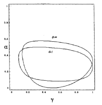
Figure 1: The contours for possible values for $\alpha$ and $\gamma$ in the exact solutions obtained for a massless scalar field and $N=3$ (in section 2); the contours are for $d=1$ and for $d=\infty$, as indicated.

In the following section we consider the exact solution to the system governed by the action (1) with non-zero $\Lambda$.

3 Solutions for a scalar field with an exponential potential

Now we turn to the $\Lambda\neq 0$ case. The field equations then take die following form:

$$\Box\phi=\frac{1}{2}a\Lambda e^{4a\phi/(D-2)}$$ (33)

$$R_{MN}=\frac{4}{D-2}\nabla_{M}\phi\nabla_{N}\phi+\frac{\Lambda}{D-2}e^{4a\phi/(D-2)}g_{MN}\,.$$ (34)

We use the same ansätze for the metric and the dilaton scalar field as in the previous section. To obtain analytic solutions we assume that the equations (9–14) are unchanged even if there is a potential term. This assumption with the homogeneous cosmological solution [10].

We find that the assumption requires two constraints on the field variables as follows:

$$T=S\qquad\mbox{and}\qquad\left(\frac{\Delta}{\sigma^{2/(d+1)}}e^{4a\phi/(D-2)}\right)^{\prime}=0\,.$$ (35)

The differential equations including the scale factor, which correspond to (5–8), are reduced to:

$$\ddot{\phi}+(D-1)\frac{\dot{S}}{S}\dot{\phi}=-\frac{1}{2}a\Lambda\left(\frac{\Delta}{\sigma^{2/(d+1)}}e^{4a\phi/(D-2)}\right)$$ (36)

$$(D-1)\frac{\ddot{S}}{S}=-\frac{4}{D-2}\dot{\phi}^{2}+\frac{\Lambda}{D-2}\left(\frac{\Delta}{\sigma^{2/(d+1)}}e^{4a\phi/(D-2)}\right)$$ (37)

$$\frac{\ddot{S}}{S}+(D-2)\left(\frac{\dot{S}}{S}\right)^{2}=\frac{\Lambda}{D-2}\left(\frac{\Delta}{\sigma^{2/(d+1)}}e^{4a\phi/(D-2)}\right)\,.$$ (38)

The equation (15) becomes

$$(D-2)\frac{\dot{S}}{S}\left(\frac{1}{2}\frac{\Delta^{\prime}}{\Delta}-\frac{1}{d+1}\frac{\sigma^{\prime}}{\sigma}\right)=\frac{4}{D-2}\dot{\phi}\phi^{\prime}$$ (39)

The differential equations (9–14) remain vaild in this case. Thus they again call for the functions of $r$ as

$$\Delta(r)=1-\left(\frac{r_{0}}{r}\right)^{N-2}$$ (40)

$$\sigma(r)=(\Delta(r))^{\gamma}$$ (41)

$$\phi^{\prime}=\pm\frac{1}{2}\sqrt{\frac{\gamma(1-\gamma)}{(d+1)(N-2)}}\frac{\Delta^{\prime}}{\Delta}$$ (42)

where $\gamma$ is left undetemined in this step.

As long as the metric (4) is used, the solutions for $S$ are treated separately for $a\neq 0$ and for $a=0$.

For $a\neq 0$ we have the following solutions to (35–38)

$$S\propto t^{1/a^{2}}$$ (43)

$$\dot{\phi}=-\frac{D-2}{2a}\frac{1}{t}$$ (44)

with

$$\frac{\Delta}{\sigma^{2/(d+1)}}e^{4a\phi/(D-2)}=\frac{(D-2)(D-1-a^{2})}{\Lambda a^{4}}\frac{1}{t^{2}}$$ (45)

Note that the sign of the time derivative of $\phi$ is given definitely in this case ($\Lambda\neq 0$).

Substituting (40–44) into (39), we find that $\gamma$ is a root of the following quadratic equation

$$\frac{a^{2}(d+1)\gamma(1-\gamma)}{N-2}=\left(\frac{1}{2}(d+1)-\gamma\right)^{2}$$ (46)

and the scalar field is expressed as

$$\phi=\phi_{0}-\frac{D-2}{4a}\left(1-\frac{2\gamma}{d+1}\right)\ln(\Delta)-\frac{D-2}{2a}\ln\left(\frac{t}{t_{0}}\right)\qquad(a\neq 0)$$ (47)

where $\phi_{0}$ and $t_{0}$ are constants that are mutually related through the relation (45). The equation (46) has real solutions if and only if $a^{2}\geq(N-2)(d-1)$. This constrains the possible range of $a^{2}$ if $d\geq 2$.

Turning to the case with $a=0$, we have the solutions to (35–38):

$$S\propto e^{Ht}$$ (48)

with

$$H^{2}=\frac{\Lambda}{(D-1)(D-2)}$$ (49)

and

$$\dot{\phi}=0\,.$$ (50)

In addition it is required that

$$\gamma=\frac{1}{2}(d+1)$$ (51)

which comes from (35). For $a=0$ we obtain the exact solution only for $d=0$ and for $d=1$.

• $d=0$. Then $\gamma=\frac{1}{2}$. The scalar field is expressed as

  $$\phi=\phi_{0}\pm\frac{D-2}{4\sqrt{N-2}}\ln(\Delta)$$ (52)

  where $\phi_{0}$ is a constant.

  The metric then takes the form:

  $$ds^{2}=-dt^{2}+\Delta^{1/(N-2)}(r)S^{2}(t)\left[\frac{dr^{2}}{\Delta(r)}+r^{2}d\Omega_{N-1}^{2}\right]\,.$$ (53)

• $d=1$. Then $\gamma=1$. The scalar field is constant everywhere,

  $$\phi=\phi_{0}\,.$$ (54)

  The metric then looks like

  $$ds^{2}=-dt^{2}+S^{2}(t)\left\{\frac{dx^{2}}{\Delta(r)}+\Delta^{2/(N-2)}(r)\left[\frac{dr^{2}}{\Delta(r)}+r^{2}d\Omega_{N-1}^{2}\right]\right\}\,.$$ (55)

The global structure of the spacetime expressed by the exact solutions will be examined in the subsequent section.

4 The global structure of the spacetime

We examine the global property of the spacetime described by the solutions obtained in sections 2 and 3. Here we take the $d$-dimensional space as an extra space, and so we study the ($N+1$)-dimensional spacetime as a physical spacetime. Therefore we will concentrate attention on the time and radial part of the metric. Furthermore, it is useful to transform the time coordinate $t$ into $\eta$, which satisfies

$$d\eta^{2}=\frac{dt^{2}}{S^{2}(t)}\,.$$ (56)

Then the ($\eta,r$) part of the metric is expressed as

$$ds^{2}=S^{2}(\eta)\left[-\sigma^{-2/(d+1)}(r)\Delta(r)d\eta^{2}+\frac{\sigma^{2/(N-2)}(r)}{\Delta(r)}dr^{2}\right]\,.$$ (57)

Here we must recall

$$\Delta(r)=1-\left(\frac{r_{0}}{r}\right)^{N-2}\qquad\mbox{and}\qquad\sigma(r)=(\Delta(r))^{\gamma}$$ (58)

where $r_{0}$ is an arbitrary constant.

Using this ‘conformally invariant time coordinate’ $\eta$, the scale factor $S$ in the case with $\Lambda=0$, treated in section 2, can be written as

$$S(\eta)=(A\eta+B)^{\alpha/(1-\alpha)}$$ (59)

where $A$ and $B$ is arbitrary constants. We remember that there is a rehtion between $\alpha$ ard $\gamma$, which can be obtained from (20–22),

$$N\alpha^{2}+\frac{(1-N\alpha)^{2}}{d}+\frac{(d+1)(N-2)}{(D-2)\gamma(1-\gamma)}\left(\frac{1}{2}(1-\alpha)-\frac{D-2}{d+1}\alpha\gamma\right)^{2}=1\,.$$ (60)

For the $\Lambda\neq 0$ treated in section 3, the relations among the several constants take different forms. In the coordinate system that includes the conformally invariant time, the expressions for the solutions take dissimilar forms for $a\neq 1$ and for $a=1$.

For $a\neq 1$, the solutions can be written as

$$S(\eta)=(A\eta+B)^{-1/(1-a^{2})}$$ (61)

$$\phi=\phi_{0}-\frac{D-2}{4a}\left(1-\frac{2\gamma}{d+1}\right)\ln(\Delta)+\frac{(D-2)a}{2(1-a^{2})}\ln(A\eta+B)$$ (62)

with

$$\frac{a^{2}(d+1)\gamma(1-\gamma)}{N-2}=\left(\frac{1}{2}(d+1)-\gamma\right)^{2}\qquad(0<\gamma<1)$$ (63)

$$e^{4a\phi_{0}/(D-2)}=\frac{(D-2)(D-1-a^{2})}{\Lambda(1-a^{2})^{2}}A^{2}$$ (64)

where $A$, $B$ and $\phi_{0}$ are constants. The value for $a^{2}$ must be greater than $(N-2)(d-1)$, for the equation (63) has real roots.

For $a=1$ we find the form:

$$S(\eta)=e^{h(\eta-\eta_{0})}$$ (65)

$$\phi=\phi_{0}-\frac{1}{4}(D-2)\left(1-\frac{2\gamma}{d+1}\right)\ln(\Delta)+\frac{1}{2}(D-2)h(\eta-\eta_{0})$$ (66)

with

$$\frac{(d+1)\gamma(1-\gamma)}{N-2}=\left(\frac{1}{2}(d+1)-\gamma\right)^{2}\qquad(0<\gamma<1)$$ (67)

$$e^{4\phi_{0}/(D-2)}=\frac{(D-2)^{2}}{\Lambda}h^{2}$$ (68)

where $h$, $\eta_{0}$ and $\phi_{0}$ are constants. Incidentally, the equation (67) has real roots only for $d=0,1$ or $d=2$ and $N=3$.

The structure of the spacetime singularity involved in this exact solution is as follows: the timelike singulality is located at $r=r_{0}$, regardless of the presence of $\Lambda$ and of the value for $a$. However, the property of another ‘cosmological’ singularity depends on the value for $\Lambda$ and $a$.

Let us consider the contracting universe, i.e. the case with the scale factor decreasing with time. This corresponds to choosing $A<0$ in (59) and $A>0$ in (61), and $h<0$ in (65). We further assume that the values of constants $B$ and $\eta_{0}$ are zero.

For $\Lambda=0$ the spacelike singularity is located at $\eta=0$, which is just the ‘big crunch’ singularity. The range of the cosmological time is $-\infty<\eta<0$. The spacelike singularity lies at $\eta=0$. Inward going radial light rays reach either the timelike or the spacelike singularity, while any outward going radial light rays reach the null singularity.

On the other hand, for $\Lambda\neq 0$, the global structure of the singularities depends on the value of $a$ (see figure 2).

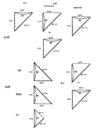
Figure 2: The schematic view of the global property of the spacetime described by the exact solutions obtained in sections 2 and 3.

For $a>1$ the global structure of the singularities is the same as the case of $\Lambda=0$. The spacelike singularity lies at $\eta=0$ (the range of $\eta$ is $-\infty<\eta<0$).

For $a=1$ there is a null singularity at $\eta=\infty$ (the range of $\eta$ is $-\infty<\eta<\infty$) [15]. Inward going light rays hit the timelike singularity at $r=r_{0}$, while any outward going light rays reach the null singlarity.

For $0<a<1$ the cosmological singularity is still null. But the range of the cosmic time is $0<\eta<\infty$.

For $a=0$ there is no other singularity besides the timelike one at $r=r_{0}$, because the spacetime is asymptotically de Sitter space in this case.

Next we examine apparent horizons in these spacetimes. It is significant to study the property of apparent horizons, especially when the metric is not static. The hiding of singularities by apparent horizons may imply the formation of black holes in many cases, for example.

An apparent horizon is lhe surface defined by

$$g^{MN}R,_{M}R,_{N}=0$$ (69)

where

$$R(\eta,r)\equiv S(\eta)r\sigma^{1/(N-2)}(r)\,.$$ (70)

In our case the equation (69) leads to

$$\frac{1}{S}\frac{dS}{d\eta}=\pm\frac{1}{r}\left[1-(1-\gamma)\left(\frac{r_{0}}{r}\right)^{N-2}\right]\left[1-\left(\frac{r_{0}}{r}\right)^{N-2}\right]^{-\frac{D-2}{(N-2)(d+1)}\gamma}$$ (71)

This defines the apparent horizon in the spacetime.

The apparent horizon may be spacelike, null, or timelike in different regions in general cases. The property can be indicated by the ratio of the slope of the apparent borizon and the null ray [8]. The absolute value of the ratio is given in our case as

$$\left|\frac{d\eta_{AH}}{d\eta_{Null}}\right|=\left|\frac{\alpha}{1-\alpha}\right|\left\{\frac{D-2}{d+1}-\frac{N-2}{d+1}\frac{[1-(r_{0}/r)^{N-2}][1+d(1-\gamma)(r_{0}/r)^{N-2}]}{[1-(1-\gamma)(r_{0}/r)^{N-2}]^{2}}\right\}$$ (72)

for the case with massless scalar. For the case with the exponential scalar potential ($a\neq 1$) equation (72) is still valid if $\alpha$ in the equation be replaced by $1/a^{2}$. For $a=1$ equation (71) merely determines the location of the timelike apparent horizon. Now, let us examine the value of (72) for each exact solution obtained in sections 2 and 3.

First we examine the massless scalar case, treated in section 2. For $d=0$, i.e. thee is no ‘extra’ dimension other than the spherically symmetric space, the equation (72) then becomes

$$\left|\frac{d\eta_{AH}}{d\eta_{Null}}\right|=1-\frac{N-2}{N-1}\frac{1-(r_{0}/r)^{N-2}}{1-(1-\gamma)(r_{0}/r)^{N-2}}<1\qquad(\mbox{for~{}}d=0,\mbox{massless})$$ (73)

since the value of $\alpha$, has been uniquely solved as $\alpha=1/N$ (24). In this case die apparent horizon is spacelike for $r>r_{0}$. Husain et al found this feature for the $N=3$ case [8], and we find there that the same characteristic of the apparent horizon holds for arbitrary dimensions of spherically symmetric space. For $d\geq 1$ the apparent horizon may be spacelike, null, or timelike in different regions, in general. We can, however, and a set or parameters ($\alpha$ and $\gamma$) which allows a spacelike apparent horizon in all regions. One cannot choose a set of the pammeters that admits a timelike apparent hoizon in all of the spacetime region, except for $N=3$ and $d\geq 2$.

Next we turn to the case with $\Lambda\neq 0$. The property of the apparent horizon depends on $a$ as well as $N$ and $d$. It is classified into four cases:

• $a=0$. To require an exact solution of the type we have considered in this paper, the allowed values for $d$ are $d=0$ and $d=1$. For each case the apparent horizon is timelike, except at $\eta=0$, $r=r_{0}$.

• $0<a<1$. In this case $d=0$ and $d=1$ are permitted as well. The apparent horizon may be timelike, null, or spacelike in a different region. But in the viciniy of $r=r_{0}$ and at spatial infinity the apparent horizon is always timelike.

• $a=1$. The allowed values for $d$ are $d=0$, $d=1$, and $d=2$. Further, for $d=2$ only $N=3$ is pemitted. For each case the apparent horizon is timelike everywhere in the spacetime.

• $a>1$. In this case any value for $d$ is permitted. but the value for $N$ is restricted by $a$ and $d$ for $d\geq 2$ through the inequality $a^{2}\geq(N-2)(d-1)$. The apparent horizon may be timelike, null, or spacelike in a different region. For a sufficiently large $a$ the apparent horizon becomes spacelike everywhere.

The schematic view of the global structue of the spacetime represented by our exact solutions is exhibited in figure 2. The cases in which the spacelike apparent horizon covers the future singularity can be regarded as models of a gravitational collapse, provided that the timelike singularity can be ignored.

5 Masses for the spherical system

In this section we evaluate the mass of the self-gravitating system of a scalar field described by the exact solutions obtained in section 2.

In the present analysis we adopt the exact solutions with $d=0$, which describes spherically symmetric spacetimep in this case the exact solution can be regarded as a model of gravitational collapse, since the future spacelike singularity is covered by the apparent horizon. The mass can be defined by local variables in the spherically symmetric system [16]:

$$m(\eta,r)=\frac{(N-1)A_{N-1}}{16\pi}R^{N-2}(1-g^{MN}R,_{M}R,_{N})$$ (74)

where $A_{N-1}=2\pi^{N/2}/\Gamma(N/2)$ and $R$ is defined by (70).

On the apparent horizon, the mass can be written in the following form:

$$M_{AH}=\frac{(N-1)A_{N-1}}{16\pi}\left(\frac{|A|}{N-1}\right)^{\frac{N-2}{N-1}}\frac{r^{N(N-2)/(N-1)}[1-(r_{0}/r)^{N-2}]^{2\gamma}}{[1-(1-\gamma)(r_{0}/r)^{N-2}]^{(N-2)/(N-1)}}\,.$$ (75)

This expression exhibits a complicated form, which depends non-trivially on the spacetime dimension.

The exact solution obtained in section 2 may not be appropriate for a model of gravitational collapse, because of the singular behaviour of the scalar field configuration as an initial condition. Our result, however, suggests that some physical quantities may depend on the space dimension. Thus we also feet interest in numerical study of the higher-dimensional gravitating system.

6 Conclusion

In this paper we have given exact solutions for a spherical collapse driven by a scalar field with an exponential potential in $D$-dimensional spacetime. The solutions describe evolution of a scalar field configuration in the background metric of a product of a spherically symmetric space and an internal space. This solution could be generalized for various supergravity models, which include dilaton fields.

References

- [1] D. Kastor and J. Traschen, Phys. Rev. D47 (1993) 5370. D. R. Brill, G. T. Horowitz, D. Kastor and J. Traschen, Phys. Rev. D49 (1994) 840. D. A. Brill and S. A. Hayward, Class. Quant. Grav. 11 (1994) 359.
- [2] J. H. Horne and G. T. Horowitz, Phys. Rev. D48 (1993) R5457. T. Maki and K. Shiraishi, Class. Quant. Grav. 10 (1993) 2171; Prog. Theor. Phys. 90 (1993) 1259.
- [3] D. Christodoulou, Commun. Math. Phys. 105 (1986) 337.
- [4] A. Salam and E. Sezgin (ed.), Supergravities in Diverse Dimensions vol. 1,2 (World Scientific, Singapore, 1989)
- [5] M. B. Green, J. H. Schwarz and E. Witten, Superstring Theory vol. 1,2 (Cambridge University Press, Cambridge, 1987)
- [6] A. I. Janis, E. T. Newman and J. Winicour, Phys. Rev. Lett. 20 (1968) 878. B. C. Xanthopoulos and T. Zannias, Phys. Rev. D40 (1989) 2564.
- [7] M. D. Roberts, Gen. Rel. Grav. 21 (1989) 907.
- [8] V. Husain, E. A. Martinez and D. Núñez, Phys. Rev. D50 3783.
- [9] T. Appelquist, A. Chodos and P. G. O. Freund (ed.), Modern Kaluza-Klein Theories (Addison-Wesley, Reading MA, 1987)
- [10] J. J. Halliwell, Phys. Lett. B185 (1987) 341. J. D. Barrow, Phys. Lett. B187 (1987) 12. J. Yokoyama and K. Maeda, Phys. Lett. B207 (1988) 31.
- [11] M. W. Choptuik, Phys. Rev. Lett. 70 (1993) 9. C. Gundlach, R. H. Price and J. Pullin, Phys. Rev. D49 (1994) 890. A. M. Abrahams and C. R. Evans, Phys. Rev. Lett. 70 (1993) 2980; Phys. Rev. D49 (1994) 3998.
- [12] P. R. Brady, Class. Quant. Grav. 11 (1994) 1255.
- [13] Y. Oshiro, K. Nakamura and A. Tomimatsu, Prog. Theor. Phys. 91 (1994) 1265.
- [14] S. B. Fadeev, V. D. Ivashchuk and V. N. Melnikov, Phys. Lett. A161 (1991) 98. V. D. Ivashchuk and V. N. Melnikov, Int. J. Mod. Phys. D4 (1995) 167.
- [15] J. H. Horne and G. T. Horowitz, Phys. Rev. D48 (1993) R5457.
- [16] W. Fischler, D. Morgan and J. Polchinski, Phys. Rev. D41 (1990) 2638; Phys. Rev. D42 (1990) 4042.
- [17] A. Strominger and L. Thorlacius, Phys. Rev. Lett. 72 (1994) 1584.
- [18] Y. Kiem, hep-th 9407100.